
Abstract
The hemodynamic response function (HRF) describes the local response of brain vasculature to functional activation. Accurate HRF modeling enables the investigation of cerebral blood flow regulation and improves our ability to interpret fMRI results. Block designs have been used extensively as fMRI paradigms because detection power is maximized; however, block designs are not optimal for HRF parameter estimation. Here we assessed the utility of block design fMRI data for HRF modeling. The trueness (relative deviation), precision (relative uncertainty), and identifiability (goodness-of-fit) of different HRF models were examined and test–retest reproducibility of HRF parameter estimates was assessed using computer simulations and fMRI data from 82 healthy young adult twins acquired on two occasions 3 to 4 months apart. The effects of systematically varying attributes of the block design paradigm were also examined. In our comparison of five HRF models, the model comprising the sum of two gamma functions with six free parameters had greatest parameter accuracy and identifiability. Hemodynamic response function height and time to peak were highly reproducible between studies and width was moderately reproducible but the reproducibility of onset time was low. This study established the feasibility and test–retest reliability of estimating HRF parameters using data from block design fMRI studies.
INTRODUCTION
The hemodynamic response function (HRF) reflects the regulation of regional cerebral blood flow in response to neuronal activation. Accurate modeling of the HRF is of interest in a number of areas of research.1, 2, 3, 4, 5 The HRF has a key role in the analysis of functional magnetic resonance imaging (fMRI) data 3 and variation in the HRF between individual subjects and between brain regions has prompted the estimation of subject-specific HRFs as a means of enhancing the accuracy and power of fMRI studies. 1 Characteristics of the shape of the evoked hemodynamic response such as height, delay, and duration may also be used to infer information about intensity, onset latency, and duration of the underlying neuronal activity. 4 Accurate estimation of the HRF is essential if fMRI is to be used to detect fine differences in the timing of neuronal activation as a means of understanding the temporal sequences of brain processes. Hemodynamic response function modeling also enables noninvasive investigation of neurovascular coupling, which changes with brain aging and may have a pathophysiological role in dementia and cerebrovascular disease.6, 7
The design of fMRI studies affects both estimation efficiency, a measure of the ability to estimate the shape of the HRF, and detection power, a measure of the ability to detect activation. Previous studies have demonstrated that there is a fundamental tradeoff between these characteristics such that designs maximizing detection power necessarily have minimum estimation efficiency and designs that achieve maximum estimation efficiency cannot attain maximum detection power.8, 9 For example, event-related designs offer high estimation efficiency but poor detection power, whereas block designs offer good detection power at the cost of low estimation efficiency. 9
A considerable body of fMRI data has already been acquired using block designs to maximize signal-to-noise ratio (SNR) and to increase the likelihood of detecting a response. In some of these studies, it would be of interest to examine the HRF explicitly even though study designs were not optimized with this in mind. In particular, studies involving large number of subjects,10, 11 multiple sites,10, 12, 13 special subject groups,11, 14 and longitudinal designs 14 would be difficult and expensive to replicate. Our specific interest in estimating HRF parameters from a block design study was stimulated by a large twin study. Here we were interested in how robustly HRF parameters could be estimated as a prelude to examining the heritability of the HRF. We approached this question first by comparing the performance of different HRF models. We then examined the test–retest reliability of HRF parameter estimation. This allowed us to identify which HRF traits remain stable over time, providing some insight into the extent to which individual parameters serve as variables reflecting a biologic trait or an experimental state. Test–retest reliability was examined in 82 healthy young adult twins tested with the same fMRI paradigm on two occasions. We examined the following parameters of the HRF: height (H), time to peak (T), full width at half maximum (W), and onset (O), respectively reflecting the magnitude, peak latency, duration, and onset latency of the localized increase in blood flow with neural activation.
MATERIALS AND METHODS
Hemodynamic Response Function Model and Features
The blood oxygenation level dependent (BOLD) fMRI signal was modeled as the convolution of the stimulus function and the HRF. Before assessing test–retest reliability in human data, we assessed the identifiability of five HRF models, summarized in Table 1, in simulated fMRI time series. Model I was the canonical HRF used in SPM8 (The Wellcome Trust Centre for Neuroimaging, London, UK), in which only the height parameter A varies. Models II, III, and IV were variants of the canonical HRF and comprise the sum of two or three gamma functions. Model V was the sum of inverse logit functions used by Lindquist et al.4, 15 The number of free parameters for model V was reduced from nine (three inverse logit functions) to seven by explicitly imposing the conditions that the fitted response should start and end at zero4, 15 noting that the other models were implicitly constrained to the same condition by their equations. Models III and V were chosen because they were previously found to have low parameter bias for event-related designs. 4 Model IV was chosen as it can model the initial dip and poststimulus undershoot. 16
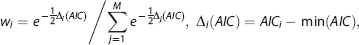
Summary of HRFs a
HRF, hemodynamic response function; k, the number of free parameters in the HRF models; LB, lower bounds; M, models; P 0 , initial values for model fittings; UB, upper bounds.
A: height; Γ: the gamma function; Ai, αi, βi, T i , and D i control the height and direction, shape, scale, shift center, and slope of the HRF, respectively.
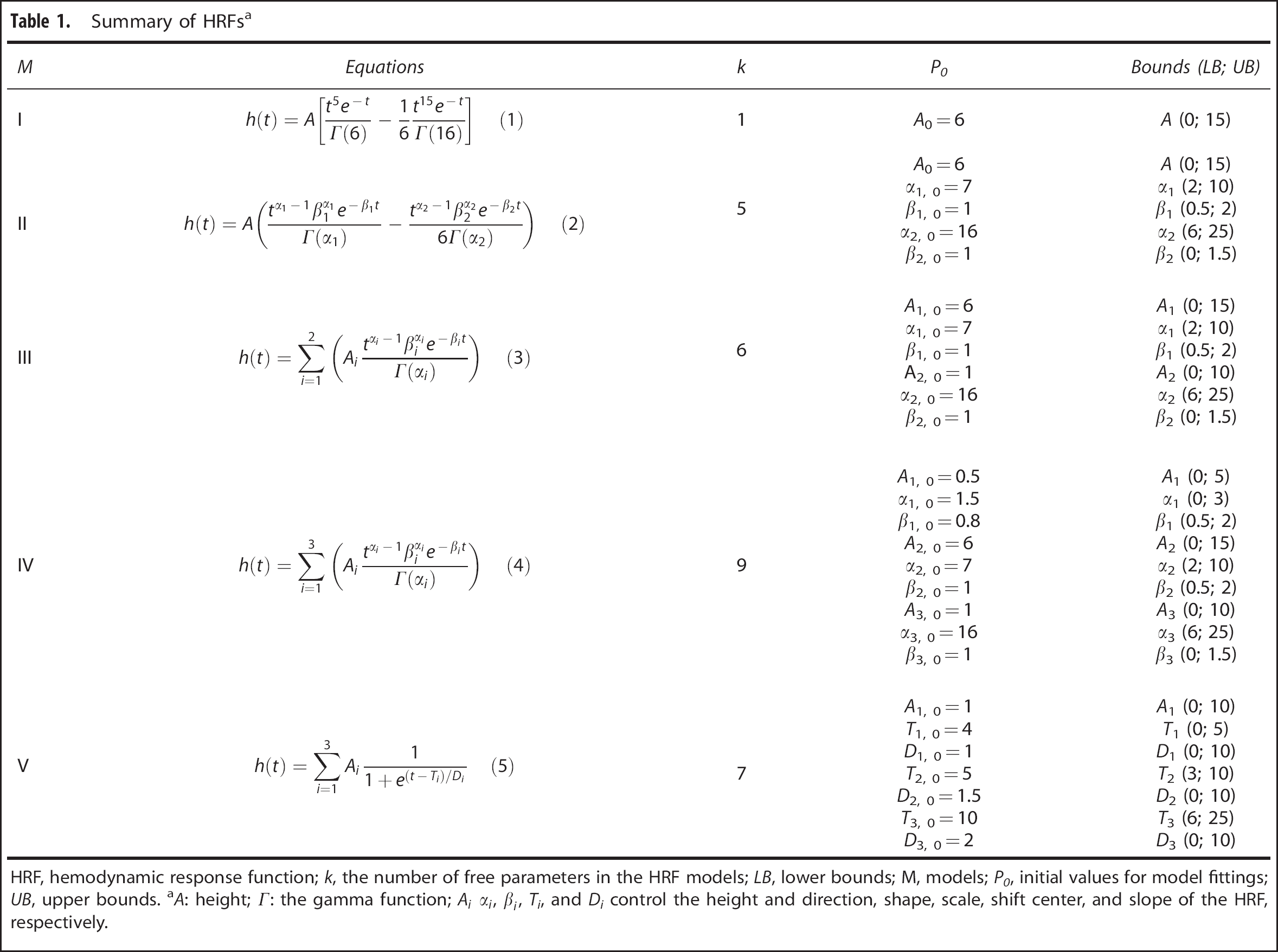
We used the following summary HRF features: height (H), defined as the maximum signal change during the peristimulus time window (30 seconds was used for this study); time to peak (T), the time taken from start time to the time when signal change reached its maximum value; full width at half maximum of the HRF (W); the onset (O), the first time point after the stimulus at which signal intensity exceeded 0.1 × H (Figure 1A).
The procedure used to simulate the functional magnetic resonance imaging (fMRI) signal time course. (
Simulation of Functional Magnetic Resonance Imaging Signal Time Course
Functional magnetic resonance imaging signal time courses were simulated using known HRFs to test the performance of different HRF models. Three ground truth HRFs were created (Supplementary Figure S1). In Simulation 1, the HRF was generated using the balloon model.17, 18 The HRF was generated using a single input at 1.5 seconds with 0.1-second duration and using typical parameters obtained empirically in a previous study: neuronal efficacy 0.54, signal decay 1.54, autoregulation 2.46, transit time 0.98, stiffness parameter 0.33, resting oxygen extraction 0.34, and resting blood volume fraction 0.06. 18 The HRF in Simulation 2 was generated using the sum of four inverse logit functions to create four segments of HRF time course:

in which A 1 =−0.2, A 2 =1.8, A 3 =−1.8, A 4 =0.2, T 1 =0.1, T 2 =4, T 3 =10, T 4 =20, D 1 =0.8, D 2 =1, D 2 =1, and D 3 =1.2. These parameters were determined empirically as generating an HRF shape with summary features (H, W, T, and O) in keeping with published values.19, 20 In Simulation 3, we used the sum of three gamma functions to generate the HRF:
in which A 1 =−0.2, A 2 =10, A 3 =−3.6, α1=1.5, α2=6.6, α3=15, β1= 0.8, β2=0.8, and β3=1. Figure 1 illustrates the procedures we used to simulate the fMRI time series. We used a block design stimulus function comprising 16 alternating blocks of rest and active conditions (8 for each condition). Each active block included 16 trials of 0.2-second duration with 0.8 seconds gap (Figure 1B). Random noise was added to achieve SNR levels of 50, 100, and 150 (Figure 1D). Noise was added without consideration of autocorrelation:

where TC is the time course of simulated fMRI data; σ is the s.d. (0.02, 0.01, and 0.067 for SNR of 50, 100, and 150, respectively); and the randn refers to a vector of pseudorandom values drawn from the standard normal distribution with the same length as TC. The range of SNR levels was selected given previous studies showing that the minimum SNR for detecting signal change in fMRI studies is 69 and the highest possible SNR is 154. 21 The simulated signal was sampled according to a typical fMRI acquisition with TR=2.1 seconds (Figure 1E). Each simulation was run 100 times.
Hemodynamic Response Function Model Selection
Hemodynamic response function modeling was performed using an in-house MATLAB (MATLAB R2010a, The MathWorks, Natick, MA, USA) toolkit, sHRF, which is publicly available at our website (http://www.cai.uq.edu.au/shrf-toolkit). The fMRI time courses were high-pass filtered with a 128 seconds discrete cosine basis set and then modeled as the convolution of the HRF (Table 1) and the stimulus function: 22

where h(t) and u(t) are the HRF and stimulus function, respectively. For the fitting we used a modified constrained Nelder–Mead Simplex algorithm that allows the use of constraints specified as parameter bounds (http://www.mathworks.com/matlabcentral/fileexchange/8277). Fitting was initialized using parameters, which generated an initial HRF shape that closely matched that of the canonical HRF. Initial values and constraints for each model are summarized in Table 1. Parameter constraints were set empirically to cover plausible HRFs with the following characteristics: an initial dip with a minimum at 0 to 3 seconds of magnitude 0% to 5%; peak BOLD signal at 2 to 10 seconds of magnitude 0% to 15%; signal undershoot with a minimum at 6 to 25 seconds of magnitude 0% to 10%. The five models cover the same space of possible HRFs except where the functional form imposes a limitation in the ability to describe the HRF. For example, Model I covers the same space for the amplitude of the BOLD peak as other models but does not allow temporal variation; Model II covers the same space for the BOLD peak and undershoot as Models III to V but the functional form does not allow an initial dip. The parameter C allows baseline adjustment of the fitted time course to match that of the simulated time series (Figure 1D). The trueness of estimated HRF parameters or the closeness of agreement between measured and ground truth values was assessed by calculating the relative deviation from the values for the HRF used to generate the simulated fMRI time course, i.e. the difference between estimated and ground truth values divided by the ground truth value. The measure of precision, or relative uncertainty, used in this study was the interquartile range of relative deviation from the values for the HRF used to generate the simulated fMRI time course. Trueness and precision were summarized using boxplots of the simulation results created in MATLAB (MATLAB R2010a, The MathWorks). The identifiability of HRF models was assessed using their Akaike weights, 23 which is the probability of each model transformed from the Akaike Information Criterion (AIC):
in which M is number of models tested and Δ i (AIC) is the difference between the AIC of each model and that of model with the smallest AIC value. In this study, we used the AIC for finite samples: 24

where RSS is the residual sum of squares between the fitted and fMRI time courses, n is the sample size, and k is the number of parameters. The HRF model with the highest AIC weight was selected for subsequent analyses of parameter estimation and reproducibility.
Parameter Estimation from Block Design Functional Magnetic Resonance Imaging Data
The noise in measured fMRI time series and sparse sampling in acquired data may lead to HRF parameter mis-specification. To examine this, we used the balloon model simulation17, 18 as the ground truth. The HRF parameters were varied in three ways: (1) H only, (2) T and O only, and (3) W, T, and O only. As illustrated in Supplementary Figure S2, varying T unavoidably changed O and varying W unavoidably changed T and O. The temporal SNR was set at 100, a typical SNR for fMRI data according to previous reports.25, 26 The highest variability across subjects observed in the literature is 25%.1, 3, 19 Hence, we varied ground truth HRF parameter values by 25%, 15%, and 10%. The simulation procedure described above in the section on HRF model selection was employed, although here only Model III was used to estimate the HRF. The simulation was executed 100 times for each type and level of parameter variation. The estimated HRF parameters were compared using the paired t-test in SPSS20 (IBM, Madison Avenue, New York City, NY, USA).
Variations in the Block Design Paradigm
To investigate the influence of variations in the block design paradigm on the trueness and precision of HRF modeling, the experimental conditions of the block design were systematically varied: (1) the number of blocks was varied from 1 to 8 with one block increments; (2) block length was varied from 4 to 16 seconds with 2-second increments; (3) stimulus duration was varied from 0.2 to 6.2 seconds with 1-second increments and a stimulus duration of 16 seconds in individual blocks (long block design) was also evaluated; (4) the gap between individual stimuli in each block was varied from 0.8 to 6.8 seconds with 1-seconds increments. Simulation of the fMRI time course was carried out as described above using the balloon model to generate ground truth, a SNR of 100, and Model III to estimate the HRF. Each simulation was executed 100 times. Trueness and precision for each paradigm were calculated as described above.
Experimental Functional Magnetic Resonance Imaging Time Course Data
The data we analyzed were acquired as part of a prior fMRI study, 11 the Queensland Twin Imaging Study. 27 Retrospective utilization of the data was approved by the Research Ethics Committee of the Queensland Institute of Medical Research and The University of Queensland in compliance with the Australian National Statement on Ethical Conduct in Human Research. Functional MRI data from 30 male and 52 female healthy young adult twins of mean age 22.5±2.5 (s.d.) years were included. For all participants, the fMRI scans were repeated 2 to 6 months later (mean 117±56 days).
Participants performed the 0- and 2-back versions of the N-back working memory task. The detailed fMRI experimental procedure is described in a previous report. 28 In the N-back task, a series of numbers is presented on a screen. The 0-back condition required participants to respond to the number currently shown on the screen. The 2-back condition required participants to respond to the number presented 2 trials earlier. The number was presented for 200 milliseconds with an 800-millisecond interval between stimuli and 16 trials per block. In total, 16 alternating blocks were performed for the two conditions (eight blocks per condition).
The three-dimensional T1-weighted MR image and echo planar imaging data were acquired on a 4T Bruker Medspec whole body scanner (Bruker, Hanau, Germany). Three-dimensionalT1-weighted images were acquired using an MP-RAGE pulse sequence (TR=2500 milliseconds, TE=3.83 milliseconds, T1=1500 milliseconds, flip angle=15 degrees, 0.89 × 0.89 × 0.89 mm). For each participant, 127 sets of echo planar imaging data (TR=2.1 seconds, TE=30 milliseconds, flip angle=90, 3.6 × 3.6 × 3.0 mm) were acquired continuously during the tasks.
The fMRI data were analyzed using Statistical Parametric Mapping (SPM8, the Wellcome Trust Centre for Neuroimaging, London, UK). The first five echo planar imaging volumes were discarded to ensure that tissue magnetization had reached steady state. The spatial preprocessing included 2-pass motion correction 29 and spatial normalization to the average brain T1 template 30 implemented in SPM8. Normalized volumes were smoothed with an 8 × 8 × 8 mm full width half maximum Gaussian kernel. In a first-level analysis of individual subject data, we determined locations of activation using the general linear model with a finite impulse response basis function. The 2-back minus 0-back contrast images were then entered into a group level, random-effects one-sample t-test to identify the common activation voxels (P<0.05 with family wise error rate adjustment for multiple comparisons).
Four regions identified at the group level were selected for HRF modeling: left and right middle frontal gyrus and left and right angular gyrus (Supplementary Figure S3). Volumes of interest were defined as the overlap of an existing probabilistic atlas of each structure in stereotaxic coordinate space 31 with group activation regions. For each participant, the fMRI time course was extracted by averaging the signal intensity at each time point in the voxels with the top 12.5% of SPM t statistics within each VOI. The top 12.5% is used here to accommodate individual variation in the pattern of functional activation within each VOI. The threshold was selected empirically as the value when the extracted time course stabilized as the percentage was decreased from 100, 50, 25, to 12.5. The HRF model selected from the simulation study was fitted to the extracted time series and used to estimate HRF parameters. Akaike Information Criterion weights were also calculated for each HRF model using real time series data.
Analysis of Test–Retest Reliability
For each brain region and each HRF parameter, the intraclass correlations of the two experimental sessions were calculated using SPSS20 (IBM) using a two-factor mixed effects model and tests of significant difference in ICC from zero performed. 32 Because the participants were biologically related monozygotic and dizygotic twins, the intraclass correlations of the HRF heights from the first-born participant in each twin pair were also evaluated to assess whether relatedness between participants affected the reliability results. The reliability of the performance measure used in the experiment has been reported previously. 11
RESULTS
Simulation Study
Figure 2 summarizes the HRF parameter estimates from the simulations. Parameter estimation was considered accurate if estimated values did not differ significantly (i.e. P>0.05) from the corresponding ground truth values. Height was estimated accurately for all SNR levels and all models except for Model V at an SNR of 50 in simulation 1 (P<0.05, one sample t-test). For Model I, T, W, and O are fixed and there is only one free parameter. Models II, III, and IV were able to estimate T, W, and O of the HRF for all noise levels accurately. Model V was able to estimate T and W accurately at all noise levels but did not estimate O accurately (P<0.05 for all three simulations). The central line and lower and upper box boundaries of the boxplots in Figure 3 respectively represent the median, 25th and 75th percentiles of 100 simulations. Models with more free parameters showed a lower precision (wider range) of parameter estimation but higher trueness (smaller relative deviation) than those with fewer parameters. Model I had the least variation but the highest bias of parameter estimation. For all three simulations, the variation and bias of parameter estimation decreased with increasing SNR for all models. For Models II to V, T was estimated with the highest precision and trueness followed by W, H, and O.

Box-and-whisker plot of the relative differences of estimated hemodynamic response function (HRF) parameters from the true values in the simulation study. Outliers were defined as exceeding three times the s.d.; all data including outliers were included in the analysis. Rows from top to bottom are the results for height (H), time to peak (T), width (W), and onset (O). Columns from left to right are results for Simulation 1 (‘balloon’ model), Simulation 2 (sum of four inverse logit functions), and Simulation 3 (sum of three gamma functions).
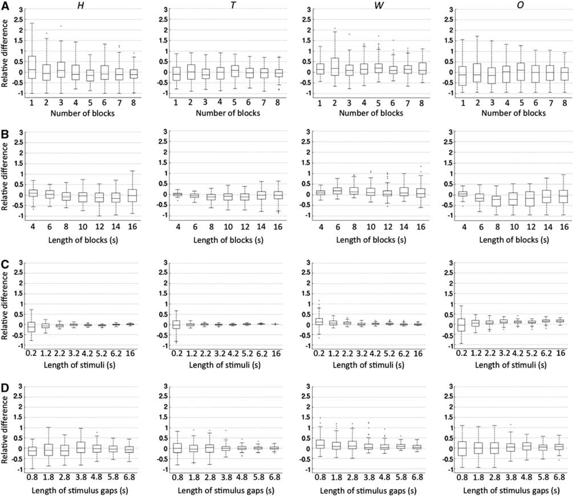
Boxplots of estimated hemodynamic response function (HRF) features with systematic variation in attributes of the block design paradigm. The columns from left to right relate to estimated height, time to peak, width, and onset, respectively. The rows from top to bottom relate to variation in the number of blocks (
Table 2 summarizes the AIC of different models for data with different noise levels. Model III had the highest AIC weights and Model I the lowest across different simulations and noise levels.
Akaike weights (W i ) for HRF models for computer simulations and real fMRI data a
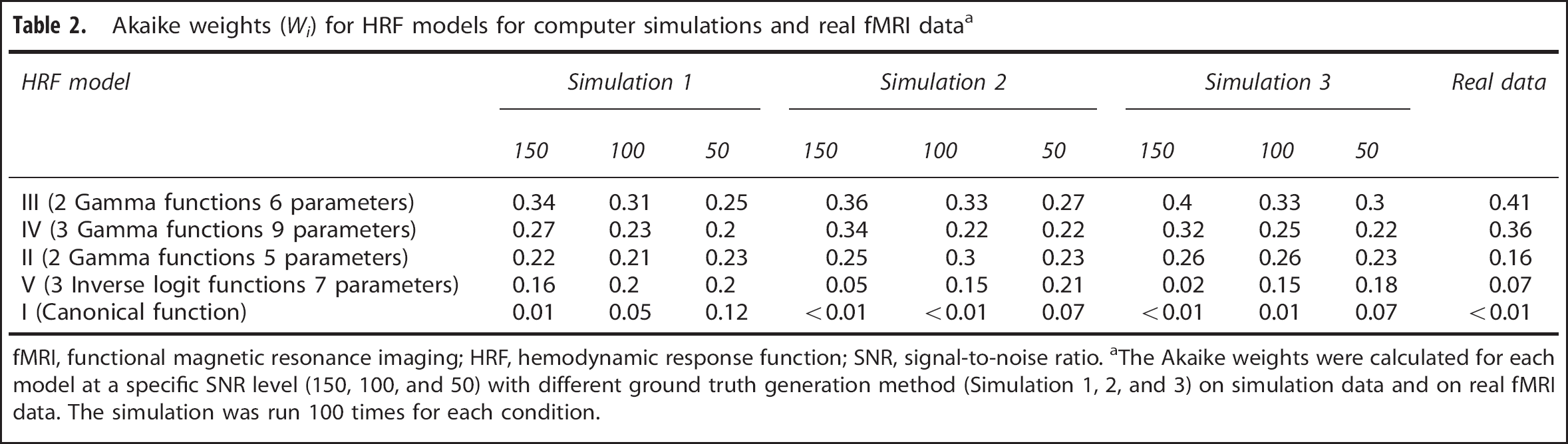
fMRI, functional magnetic resonance imaging; HRF, hemodynamic response function; SNR, signal-to-noise ratio.
The Akaike weights were calculated for each model at a specific SNR level (150, 100, and 50) with different ground truth generation method (Simulation 1, 2, and 3) on simulation data and on real fMRI data. The simulation was run 100 times for each condition.
Results for HRF parameter estimation are summarized in Table 3. The selected HRF model (Model III) was able to identify parameter differences exceeding 10% with SNR of 100. There were no instances in which significant changes in one parameter resulted from variation in another parameter.
Estimation of HRF parameter variation a
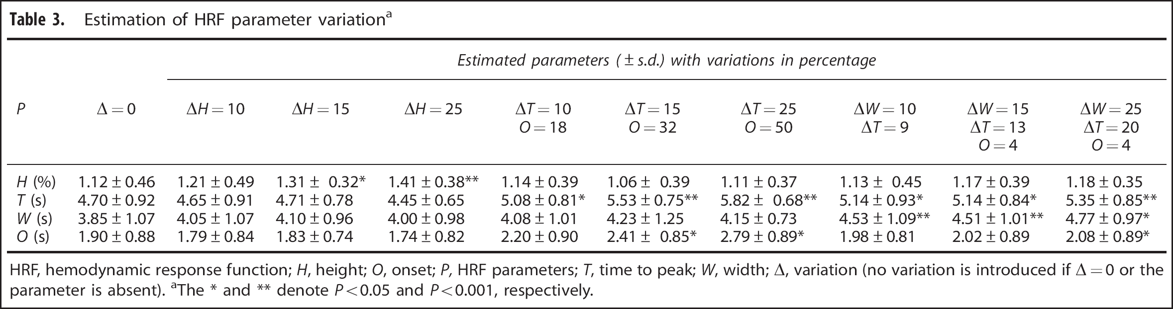
HRF, hemodynamic response function; H, height; O, onset; P, HRF parameters; T, time to peak; W, width; Δ, variation (no variation is introduced if Δ=0 or the parameter is absent).
The ∗ and ∗∗ denote P<0.05 and P<0.001, respectively.
Results of parameter estimation with different block design paradigms are summarized in Figure 3 using boxplots constructed in the same manner as Figure 2. For less than six blocks, mean estimated H, W, and O generally had relative errors greater than 0.1 and an interquartile range greater than 0.5 (Figure 3A). Trueness was similar across paradigms with different block lengths. However, precision was increased with reduced block length (Figure 3B). Both trueness and precision of parameter estimation increased with greater stimulus duration within each block (Figure 3C). Trueness and precision also increased when the gap between stimuli was increased to 3.8 seconds and remained similar with larger gaps (Figure 3D).
Real Functional Magnetic Resonance Imaging Data
Akaike Information Criterion weights for the models using real fMRI data were consistent with results from simulations (Table 2). Model III had the highest AIC weights. Activation maps between the two experimental sessions were highly reproducible (Supplementary Figure S3). Quantitative assessment of the repeatability of the activation map between two experimental sessions has been reported previously. 11 The ICC(3,1) of HRF parameters estimated in the two experimental sessions using Model III are summarized in Table 4. Height and T are highly reproducible, W is moderately reproducible, and reproducibility of O is low. The 95% confidence intervals of all parameters overlap between the two experimental sessions. Height is lower in session 2 than in session 1. A practice effect was also observed in the performance data. 11 Biologic relatedness between participants did not affect reliability results. The intraclass correlations of HRF heights from the first-born participant in each twin pair (N=41) for left and right middle frontal gyrus and left and right angular gyri were 0.64 (P<0.01), 0.58 (P<0.01), 0.63 (P<0.01), and 0.64 (P<0.01), respectively.
The ICC(3,1) of HRF parameters between the two experimental sessions a
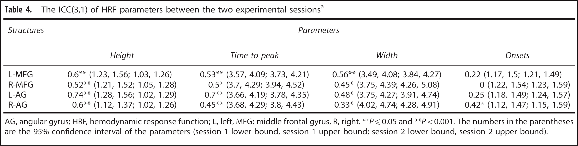
AG, angular gyrus; HRF, hemodynamic response function; L, left, MFG: middle frontal gyrus, R, right.
∗P0.05 and ∗∗P<0.001. The numbers in the parentheses are the 95% confidence interval of the parameters (session 1 lower bound, session 1 upper bound; session 2 lower bound, session 2 upper bound).
DISCUSSION
Modeling of the HRF using fMRI is a noninvasive method to investigate the brain's hemodynamic response to neuronal activation. In this study, we found that with block design fMRI paradigms, most HRF models were able to estimate HRF parameters except for Model V that had difficulty estimating onsets. The sum of two gamma functions with six free parameters had the greatest identifiability of the five models tested but the accuracy of parameter estimation varied with block design attributes. H, T, and W were reproducible between two experimental sessions.
We used computer simulations with a known ground truth to assess the performance of the HRF models. In the simulations, Gaussian noise was added at each SNR level without consideration of autocorrelation. However, fMRI noise typically exhibits temporal dependence (autocorrelation); therefore, the SNR level is slightly lower than in practice. Parrish et al 21 demonstrated that a minimum SNR of 69 is required to detect a 1% BOLD signal change with 112 image volumes. Our results were similar, showing that Models I to IV could estimate H accurately with a SNR of 50 and 122 image volumes. The simulation results for the five models showed that models with more free parameters had lower precision but higher trueness of HRF parameter estimation (Figure 3). The canonical HRF (Model I) had the least variance, but the estimated height was more likely to be biased. The tradeoff between the number of parameters and precision and trueness motivated the use of AIC weights for model selection.
A key consideration in HRF model selection is the number and nature of a priori assumptions. Recently, Lindquist et al 4 assessed the performance of different HRF models for event-related designs in terms of bias, mis-specification, and statistical power. Seven models were compared: the canonical HRF, canonical HRF with temporal derivatives, canonical HRF with temporal and dispersion derivatives, finite impulse response, smoothed finite impulse response, sum of two gamma functions, and the sum of three inverse logit functions. The study suggested the sum of two gamma functions is not optimal for fitting noisy data from event-related studies and should only be used on regions where it is known that there is signal present. 4 Our study focused on HRF modeling using block design fMRI data in which signal is present. As illustrated in the simulation study (Figure 3), models with few assumptions are more flexible or may handle HRF shapes with unexpected response behaviors more accurately than models with many fixed parameters. However, a greater number of free parameters may also lead to overfitting of noise, lowering precision. This may explain the relatively poor performance of Model V in our study. In Lindquist et al, 4 superior performance for Model V compared with gamma function models for event-related designs that have a high HRF estimation efficiency 8 and high temporal resolution (TR=0.5 seconds),4, 15 most likely reflects Model V's greater flexibility.4, 15 In contrast, in the present study of block designs with low estimation efficiency, prior knowledge implicitly encoded in the gamma function models constrained them from overfitting noisy data. We used AIC weights to judge model identifiability. The AIC is a measure of the relative goodness-of-fit of a statistical model compared with others, with a penalty given for using extra parameters. 33 The AIC with a correction for finite sample sizes was used in this study (equation (10)); the correction is minimized when the sample size is large. 24 Based on AIC values, Wagenmakers et al 23 further proposed Akaike weights, which may be directly interpreted as conditional probabilities for each model. For example, an AIC weight of 0.41 for Model III with real data in our study indicates that this model has a 41% probability of being the best model of those tested. The AIC values of different models are consistent between the simulations and real fMRI data. The results suggest that the sum of two gamma functions with six parameters is the best HRF model when it is known that there is signal present. With a typical fMRI SNR of 100, a two-gamma-function, six-parameter model can discern 15% HRF feature variation without misattributing variation in one parameter to another. Inter-and intra-subject variability of the HRF has been studied previously in event-related fMRI experiments.1, 3, 19, 34, 35, 36 In the present examination of a block design study, H, T, and W were reproducible between two experimental sessions, supporting the validity of these HRF parameters as biologic measures. The repeatability results may also provide insight into neural responses and neurovascular coupling. For example, the reproducibility of H between trials implies that the neural firing rate as well as the vascular response induced by the same task across different sessions for each individual was very similar. In previous studies,5, 37, 38 the height of the BOLD response to visual stimulation was negatively correlated with resting GABA concentration in the visual cortex. If this relationship is widespread in the brain, our results suggest that endogenous factors, such as neurotransmitter concentration, which regulate the balance between excitation and inhibition in the individual brain may also remain relatively stable. The reproducibility of T and low reproducibility of O has implications for the ability to infer synchrony and directional influence among neural populations during task performance and in the resting state from block design fMRI data. Our findings on HRF test–retest reliability, particularly for temporal parameters, are in broad agreement with results from studies optimized for HRF estimation by the use of event-related designs and long baseline periods,1, 36 in which time to peak had the greatest test–retest reliability and time when the BOLD response begins to rise steeply from baseline (similar to O in this study) had the largest test–retest variation.
In this study, we represented neural activity by the stimulus time course, an assumption underlying commonly used methods for statistical parametric mapping. To the extent that this assumption is violated, it is likely that the HRF model parameters estimated here contain a component of neural activity in addition to vascular reactivity. Several techniques have been recently proposed to dynamically filter fMRI time courses to estimate neural activity as well as the vascular response explicitly.39, 40 Application of these techniques in future studies may allow the reproducibility of the HRF to be estimated more specifically.
Many HRF models have been proposed in the literature. Our study was restricted to five models that are commonly used or have been shown in prior studies to be less susceptible to mis-specification errors (sum of inverse logit functions) or parameter bias (sum of two gamma functions). In this study, we examined vascular responses to neural activity evoked by a single cognitive function in four brain structures that demonstrated robust activation. Further studies using other activation tasks are needed to assess generalizability of our findings to other brain regions and brain functions.
Block designs are not optimal for HRF estimation and random event-related designs and m-sequence designs have been shown to have higher estimation efficiency. 9 Nonetheless, our data on model selection and on the reliability of HRF estimation should increase the utility of existing block design fMRI data. Indeed, the methodology presented in this paper will be used to analyze the heritability of HRF parameters in a large twin cohort using block design fMRI data that were originally collected to address heritability of spatial patterns of functional activation with a working memory task. 11 In our tests of the effects of varying the attributes of the block design paradigm, we found that at least six blocks are required to model the HRF accurately. The simulations showed that prolonging the length of blocks does not affect the trueness of the parameter estimation but decreases precision. This result is in keeping with HRF modeling being more sensitive to the initial increase and the final decrease of the signal than the plateau stages in the middle of block. Prolonging the block introduces additional noise reducing precision. Decreasing the frequency of stimuli in each block by increasing the gap between stimuli increases the accuracy of parameter estimation. This finding agrees with a previous theoretical model describing the tradeoff between estimation efficiency and detection power 8 in the sense that block designs with decreasing stimulus frequency in each block bear a greater resemblance to event-related designs.
In conclusion, we investigated trueness, precision, model identifiability, and test–retest reproducibility of parameter estimates for HRF models with a block design paradigm using simulated and real fMRI data. The HRF features of height, time to peak, and width were reproducible between test sessions and may be useful as measures to characterize the coupled vascular response to neural activity in individual subjects.
Footnotes
The authors declare no conflict of interest.
ACKNOWLEDGMENTS
The authors thank the twins for participating in this study, research nurses Marlene Grace and Ann Eldridge at QIMR for twin recruitment, and radiographers Matthew Meredith, Peter Hobden, and Aiman Al Najjar from the Centre for Advanced Imaging, The University of Queensland, for data acquisition, and research assistants Kori Johnson and Lachlan Strike, Queensland Institute of Medical Research, for preparation and management of the imaging files.
References
Supplementary Material
Please find the following supplemental material available below.
For Open Access articles published under a Creative Commons License, all supplemental material carries the same license as the article it is associated with.
For non-Open Access articles published, all supplemental material carries a non-exclusive license, and permission requests for re-use of supplemental material or any part of supplemental material shall be sent directly to the copyright owner as specified in the copyright notice associated with the article.