
Abstract
Brief neural stimulation results in a stereotypical pattern of vascular and metabolic response that is the basis for popular brain-imaging methods such as functional magnetic resonance imagine. However, the mechanisms of transient oxygen transport and its coupling to cerebral blood flow (CBF) and oxygen metabolism (CMRO2) are poorly understood. Recent experiments show that brief stimulation produces prompt arterial vasodilation rather than venous vasodilation. This work provides a neurovascular response model for brief stimulation based on transient arterial effects using one-dimensional convection-diffusion transport. Hemoglobin oxygen dissociation is included to enable predictions of absolute oxygen concentrations. Arterial CBF response is modeled using a lumped linear flow model, and CMRO2 response is modeled using a gamma function. Using six parameters, the model successfully fit 161/166 measured extravascular oxygen time courses obtained for brief visual stimulation in cat cerebral cortex. Results show how CBF and CMRO2 responses compete to produce the observed features of the hemodynamic response: initial dip, hyperoxic peak, undershoot, and ringing. Predicted CBF and CMRO2 response amplitudes are consistent with experimental measurements. This model provides a powerful framework to quantitatively interpret oxygen transport in the brain; in particular, its intravascular oxygen concentration predictions provide a new model for fMRI responses.
Keywords
INTRODUCTION
Neural activity causes local changes in cerebral oxygen consumption (CMRO2), blood flow (CBF), and deoxyhemoglobin concentration.1,2 This combination of neurometabolic and neurovascular coupling enables the use of hemodynamic imaging methods to infer brain activity. Of particular interest is the response to brief periods (few seconds) of neural activity, the hemodynamic response function (HRF). The stereotypical HRF permits the use of powerful linear analysis methods.
Despite the utility of the HRF for quantifying brain activity, the mechanisms of transient oxygen transport remain poorly understood. There are at least three controversial issues. First, the role of venous volume changes is not clear, particularly in response to brief neural stimulation.3–5 Second, there is disagreement about the relative role of capillaries and arterioles in oxygen transport to tissue.6–8 Third, experiments in oxygen mass balance have sometimes shown that metabolic consumption is insufficient to account for global oxygen loss from the vasculature. It was therefore suggested that tissues at or adjacent to the vascular wall may consume the missing oxygen.9,10 Thus, questions remain about oxygen transport both in steady state and as a consequence of brief stimulation.
Various computational models have attempted to explain the dynamics of the HRF. The most popular model is the ‘balloon model,’ which postulates non-linear venous inflation with increased CBF;3,11 such models have become increasingly sophisticated and complex.12,13 These models provide accurate fits for the HRF. However, recent brief stimulation experiments demonstrate significant arterial volume changes with minimal venous volume changes.4,5,14 Accordingly, a ‘proximal-integration’ hypothesis was suggested, in which a vasodilation signal proximal to neural activity rapidly propagates upstream to pial arteries. 15 These arterial transients, rather than venous compliance, must have a key role in the dynamics of the HRF. Accordingly, for brief neural activity, the current theoretical framework around non-linear venous dilation needs to be revised.
Previously, we proposed a transient oxygen-transport model driven by upstream arterial flow changes. 16 We asserted that such dilation could generate pressure fluctuations in pial arteries that couple to microvascular flow changes. We described this flow response using a lumped linear model. The earlier model was able to fit a heterogeneous set of transient tissue oxygen time-series responses measured in cat visual cortex. 17 However, this model had some limitations. Specifically, it did not include the dynamics of oxygen dissociation, used only a rectangular function for the CMRO2 response, and did not operate from a fixed steady-state condition. Moreover, without considering hemoglobin oxygen dissociation, the model was unable to predict absolute oxygen concentration.
Here, we substantially extend the previous model. First, the transport model now includes realistic treatment of oxygen dissociation, which enables calculation of oxygen concentration in absolute units and a full treatment of steady-state oxygen mass balance. Second, the model can thereby start from a realistic steady state, decoupled from the transient dynamics. Previously, the steady-state conditions were linked to the transient modeling by modifying the transport geometry. Third, we include the possibility of wall consumption (or similar loss mechanism), which can be necessary to obtain oxygen mass balance depending upon the chosen set of the steady-state parameters. Finally, instead of using a rectangular function for transient CMRO2 response, the model uses a gamma function to match experimentally observed temporal characteristics of the CMRO2 response. This feature provides physiologic insight into how the CMRO2 response affects the HRF.
All in all, we provide a tractable oxygen-transport model based on prompt arterial dilation evoked by brief neural activity capable of predicting absolute oxygen concentration. Our model provides accurate and detailed predictions of transient extravascular oxygen time courses with heterogeneous combinations of initial dips, hyperoxic peaks, undershoots, and ringing in cat visual cortex using only six optimization parameters. It also provides CBF and CMRO2 responses that explain the physiology of the HRF in detail.
MATERIALS AND METHODS
Transport Model
A one-dimensional (1D) cylindrical geometry is employed to represent a single, stereotypical element of the microvascular network in cerebral cortex, a ‘vascular unit’ for oxygen transport starting with small arterioles through its associated capillary beds (Figure 1A). Experimental findings on oxygen transport in rat brain demonstrated that oxygen transport in the brain occurs principally from very small vessels (eg., small arterioles and capillaries).8,18 Accordingly, we assumed that the oxygen transport begins principally from third-order arterioles. These studies also motivated our assumption of a uniform cylindrical geometry.
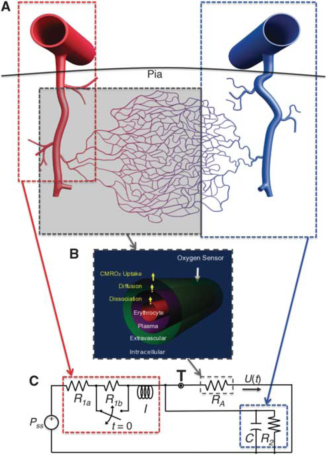
The oxygen-transport and flow models. (
Our transport model is based on the mechanisms of flow and diffusion in multiple concentric cylindrical compartments. We illustrate the relevant dynamics with a simplified example with only two compartments: intravascular and extravascular. Temporally variable CBF occurs in the intravascular compartment (subscript i). In this 1D geometry, CBF is interchangeable with flow speed in the z direction, U(t), because the cross-section area of the intravascular compartment is constant. In the extravascular compartment (subscript e), the flow is assumed to be zero, but diffusion occurs between the plasma and extravascular compartments. Consider a differential element of length (Sz) in our compartmental 1D geometry. Within the blood vessel, the oxygen concentration at spatial position z is given by Qi(z, t). Flow delivers oxygen at the rate of U(t)Qi(z, t)ᴨR 2 , where R is the blood vessel radius, while diffusion delivers oxygen to the extravascular compartment at a rate that is proportional to the transmural concentration difference, 2pRδz(Qi-Qe)D/w, where D is the oxygen diffusion co-efficient and w is the thickness of the vessel wall. Altogether, the differential oxygen mass balance in the intravascular compartment becomes:

Thus, the rate of change of oxygen is the sum of oxygen delivered by flow balanced by losses from transmural diffusion. These concepts form the core of our analysis.
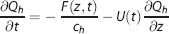
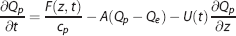
In the current model, we use a concentric three-compartment geometry to include the dynamics of oxygen dissociation (Figure 1B). This represents the small arterioles and capillaries where oxygen transport mainly occurs. The intravascular compartment is separated into erythrocyte (subscript h) and plasma (subscript p) compartments. The contribution of oxygen dissociation is modeled using a flux term F(z, t) between these two compartments. Oxygen transport through diffusion again links the plasma and extravascular compartments. We also want to test a wall-consumption hypothesis,7,10 which postulates that the vessel wall (or apposed tissue such as smooth muscle) can consume some fraction of the oxygen diffusing across the transmural boundary. Accordingly, we introduce a wall consumption term, where parameter W modulates a parallel path of diffusion from the plasma to the extravascular compartment. With this combination of features in a three-compartment system (erythrocyte, plasma, and extravascular), mass balance yields:
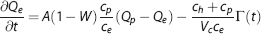
where is volume per unit length, A is a diffusion rate constant proportional to D, and Vc is an effective blood-volume fraction for small arterioles and capillaries (Appendix 1).
Equation (2) states that the rate of change in erythrocyte oxygen concentration is balanced with oxygen-dissociation efflux to the plasma compartment (first term on the right side) and oxygen delivery in z-direction by flow (second term). Equation (3) states that the rate of change in plasma oxygen concentration corresponds to oxygen-dissociation influx from the erythrocyte compartment (first term on the right side), transmural diffusion to the extravascular compartment (second term), and oxygen delivery by flow (third term). Equation (4) states that the rate of change in extravascular oxygen concentration is determined by transmural diffusion from the plasma compartment that is a combination of conventional diffusion and wall consumption (first term on right side), and oxygen metabolic consumption, T(t) (second term). These three mass-balance equations describe the transport of oxygen through our model geometry.
Analytic solution of this set of equations is not possible in general, so we utilized numerical methods. Hemoglobin oxygen dissociation is often approximated using the Hill equation, 19 which has a sigmoidal form that complicates numerical solution of the mass-balance equations. We utilized a quadratic fit to the Hill equation to describe oxygen dissociation within the range of oxygen concentrations relevant to in vivo cerebral microvascular physiology. Using this approximation, the oxygen-dissociation flux term F(z, t) can be eliminated to yield a simplified pair of equations that can be readily solved using standard methods of numerical integration (Appendix 1).
Setting all the time derivatives to zero in steady state yields a pair of ordinary differential equations that can be solved analytically (Appendix 2). The results relate the blood vessel length (L) and wall consumption (W) to a set of experimental parameters obtained from the literature (Table 1). The steady-state solution provides the starting point for the evaluation of the dynamic changes evoked by neural stimulation.
Steady-state parameters

CBF, cerebral blood flow; CBV, cerebral blood volume; CMRO2, cerebral oxygen consumption.
The choice of parameters strongly affects the steady-state solution, so we must consider our choices carefully. In particular, there is uncertainty or wide variability in measured values for steady-state CMRO2 (Γ ss ), steady-state CBF (Uss), and initial transmural gradient (σ). For steady-state CMRO2 (Γ ss ), we choose a nominal value of 0.03 mmol/L/s for gray matter, as measured by positron emission tomography (PET),20,21 but reported values in human and non-human brains vary from 0.006 to 0.056 mmol/L/s.2,22,23 Therefore, we test a range of values (0.01 to 0.05 mmol/L/s). Steady-state CBF (Uss) for the various high-order arterioles and capillaries also vary over a wide range, but our model simplifies the geometry to a single cylinder with fixed diameter. We chose a nominal value of Uss = 1.84 mm/s based on experimental findings24,25 together with a weighting procedure similar to that used for the calculation of effective blood-volume fraction (Appendix 1). We also experiment with three-fold variation around this value. Initial transmural gradient (σ) is the oxygen-concentration ratio between the plasma and extracellular compartments at the proximal end of the cylinder. We choose a nominal value of 0.1 based on measurements in rat brain using polarographic probes,18,26 but reported measurements of this parameter have also varied substantially. We therefore experiment with a range of 0.1 to 0.5. Steady-state modeling is performed over these ranges of the three parameters to examine their effects on blood-vessel length and wall consumption. Also, modeling of the responses to neural stimulation is performed over these ranges of the three steady-state parameters to examine their effect on fits to our own experimental observations.
CBF and CMRO2 Response
We model the transient response in blood flow based upon the experimental findings that suggested the proximal-integration hypothesis. 15 During transient neural activity, vasodilation starts in the microvasculature local to the neural activity (Figure 2). This dilation causes a local increase in blood flow that generates mechanical shear stress on the vascular wall. This shear stress, in turn, produces a back-propagating wave of vasodilation into the upstream arterial vasculature, which then creates an upstream pressure fluctuation. The time scale of this process is fast (~ 1 second), 14 so that it can be treated as an impulse on the time scale of the blood-flow dynamics.

Sequence of the flow response caused by proximal integration. (1) A brief period of neural activity triggers increased microvascular flow, leading to (2) a wave of vasodilation that propagates up to (3) the pial arteries. This transient dilation, in turn, drives (4) a pressure fluctuation that couples to (5) a downstream viscous-flow response.
We use a lumped linear flow model to describe the effects of this pressure fluctuation in the pial arteries (Figure 1C). It has been shown that an inertial element is necessary when considering hemodynamics at the scale of the pial arteries. 27 We, therefore, model the upstream vasculature by including an inertive element to represent the kinetics of blood flow (red outline). The effects of the downstream venous vasculature are modeled by including resistive and compliant elements to represent its aggregate dynamics (blue outline). This lumped linear flow model is also known as a 4-element windkessel (FEW), which has been widely used for cardiovascular flow modeling. 27 The flow response in this linear system is described by an ordinary differential equation:

where I is the inertance, RFEW is resistance, C is compliance, and P is pressure. Here, the first term corresponds to Newton’s second law, and inertance is a geometric scaling of mass. The second term reflects frictional losses, while the third term corresponds to energy storage in the compliance of the downstream venous vasculature. Note that this equation is similar to those used in previous modeling efforts that included a damped harmonic oscillator to describe the flow response.28,29 In our case, the transient arterial response is modeled by closing the switch across R1b briefly, representing a vasodilation that decreases the upstream vascular resistance (Figure 1C). Because of inertial effects, this vasodilation creates a positive pressure fluctuation. The arterial pressure response given by the solution of Equation (5) couples linearly to the CBF through the small arterioles and capillaries in which oxygen transport predominantly occurs (gray shaded region in Figure 1A and gray outline in Figure 1C). This can be demonstrated from the analytic solution for viscous flow in a 2D cylindrical geometry (see Supplementary Material).
Solution of Equation (5) thus gives the microvascular flow response, which has two forms depending upon the time constants of the system:

Three parameters characterize the flow impulse response: frequency (f), damping time (τ), and amplitude (U1). Note that the underdamped form has an oscillatory character, which can model ringing in the flow response, while the overdamped form is the sum of exponential decays and does not oscillate.
Spatially, uniform oxygen uptake from the surrounding tissue is assumed along the whole length of the modeled cylindrical blood vessel. In several experiments, the CMRO2 response to brief neural activity consists of a prompt fast increase and relatively slow decay.30–32 A gamma function is therefore used to model the transient CMRO2 response:
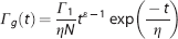
where N is a normalization constant, damping time is η, shape coefficient is ε, and amplitude is Γ1. The damping time mostly affects the decay of the transient CMRO2 change, while the shape coefficient principally affects its rise time.
We assume that these two transient impulse responses in CBF and CMRO2 are driven by the visual stimulus, which we model as a rectangular pulse, rect(t/T −0.5), where T = 4 seconds is the stimulus duration. The full responses are then obtained by convolution with the rectangular pulse: Up(t) _ UFEW(t)**rect(t/T −0.5), and Γ p (t) = Γ g (t)**rect(t/T −0.5), where ‘**’ denotes convolution. CBF and CMRO2 are defined as U(t) = Uss + Ua(t) and Γ(t) = Γ ss + Γ a (t), respectively, the sum of steady-state components (Uss, Γ ss ) and transient components (Ua(t), Γ a (t)) evoked by the neural activation.
Fitting Tissue-Oxygen Measurements
We applied the model to experimental tissue-oxygen measurements obtained in area 17 of cat visual cortex. 17 Briefly, in those experiments, a combined microelectrode and polarographic sensor was used to measure the dynamics of neural activity and tissue oxygenation, respectively. Spiking activity recorded with the electrode from a particular local cell was used to guide the visual stimulus selection. Stimuli were drifting full-contrast gratings applied for 4-second periods to the receptive field of each local cell. There were eight stimulus conditions: seven grating orientations that formed a rough orientation-tuning curve, including the ‘preferred’ (largest evoked spiking) and orthogonal orientations presented to the dominant eye; only the preferred orientation was presented to the non-dominant eye. The field of sensitivity of the oxygen sensor was a sphere ~60 μm in diameter. Both neuronal and oxygen measurements were collected for 40-second periods starting 10-seconds before stimulus onset. The measurements gave only relative rather than absolute oxygen concentration dynamics.
We obtain the full transient evolution of the system starting from a particular steady state. Heun’s modified Euler’s method 33 is used to accurately evolve numerical solutions of the transient concentrations in each compartment. The system is spatially gridded with at least 80 steps between 0 and L along z; more grid points are used if needed to enforce a maximum step size of 20 μm. Time step is chosen as Δt = 0.2Δz/Uss, to accurately resolve steady-state convection. We evolve this transient solution for 0 to 25 seconds to enable comparison with our experimental data. We assume that the experimental polarographic measurement corresponds to oxygen concentration at the distal end of the cylinder in the extravascular compartment. Because the sensor measured oxygen concentrations produced by many local microvessels within the gray matter parenchyma, we average oxygen concentration over ~60 μm at the distal portion of the cylinder, which is equivalent to both the sensitive region of the polarographic probe, and the mean length of a capillary segment: 34 see Discussion. The computational model is coded in Matlab (Mathworks, Natick, MA, USA). To reduce the computing time, the main numerical integration calculation is coded in C and linked to Matlab.
Optimization and Data Analysis
We use the model to fit the 166 individual oxygen-concentration time series 17 described above. Model fits start from a particular choice of steady-state, and best-fit transient response predictions are then computed using six optimization parameters. Three parameters specify a CBF response: frequency f; damping time η; and amplitude U1, and three more specify a CMRO2 response: damping time η; shape coefficient ε; and amplitude Γ1. The six parameters are initially adjusted manually to approximately match the predicted oxygen concentration to experimental measurements associated with maximal neuronal activity in each cell. Using these parameters as a starting point, we then use non-linear optimization 35 to improve the fits to the measurement time series across all stimulus conditions of that cell by minimizing the negative sum of the log likelihood of the model at all time points. The likelihood is calculated assuming a Gaussian error distribution defined by the mean and standard error of the mean obtained from the experimental data. The quality of a fit is assessed by computing the mean deviation between the fit of the measurement as a fraction of the experimental standard error. Fits where the mean deviation is < 1 are considered successful.
For successful fits, we also investigate correlations between model optimization parameters, and the observed neuronal activity. Neuronal activity is calculated as the difference between the mean of the steady-state neuronal firing rate and the mean firing rating during stimulus presentation. Because each electrode sampled individual units, there was substantial cell-to-cell variability in the neuronal firing rates (a population average across columns would show much less variability). To deal with this variability, we normalize the measured neuronal firing rate and each parameter by a ‘cocktail mean’ for each cell, that is, the mean value of each parameter across all stimulus orientations.
RESULTS
Steady-State Conditions
We use our analytic result for the steady-state intra- and extravascular spatial oxygen concentrations (Appendix 2). Both concentrations decrease from proximal to distal, typically starting with a non-linear exponential decrease at high concentration, followed by a comparatively linear decrease at lower concentrations (Figure 3). The steady-state plasma and extravascular concentration in the spatial sampling region (blue shading) are 0.053 and 0.044 mmol/L, respectively (38.13 and 31.65 mm Hg).

Normalized spatial oxygen concentrations in plasma and extravascular compartments for our nominal steady state. Proximal plasma concentration, 0.093 μmol/L (66.9 μm Hg) at z = 0 was calculated from hemoglobin dissociation assuming an erythrocyte concentration of 8.56 μmol/L. From proximal to distal, there is a non-linear decrease at high concentrations, followed by a relatively linear decrease at lower concentrations. Blue shaded region represents the spatial sampling used to compare modeling results with the measured transient extravascular oxygen concentrations.
We investigate the effect of the initial transmural gradient (σ), steady-state CMRO2 (Γ ss ) and CBF (Uss) on cylinder length (L) and wall consumption (W) within the ranges of experimental measurements on the steady state (Figure 4). For Γ ss at its nominal value (0.03 mmol/L/s), changes of L and W are examined as a function of .ss and s (Figures 4A and 4B). L is dependent on both Uss and σ. For small σ = 0.1, L increased from ~100 to 1,000 μm as .ss varied from 0.61 to 5.52 mm/s, while for high s −0.5, L increases over a much smaller range from ~30 to 230 μm (Figure 4A). W depends only upon transmural gradient and is independent of flow speed. Increasing σ from 0.1 to 0.5 causes a non-linear increase in W from 0.19 to 0.84 (Figure 4B).
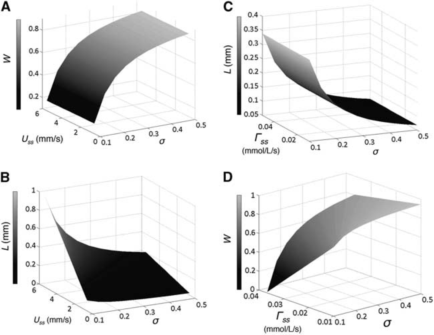
Effects of three parameters on wall consumption (W) and cylinder length (L) in steady state. Panels
Figures 4C and 4D show the effects of varying Γ ss and σ at the nominal flow speed, Uss = 1.84 mm/s. L decreases monotonically from B340 to 70 μm with increasing s and is independent of Γ ss (Figure 4C). W varies with both transmural gradient and steady-state CMRO2. For small σ = 0.1, wall consumption decreases rapidly from B0.7 to 0.01 as Γ ss increases from 0.01 to 0.037 μmol/L/s. However, for large s_0.5, the model predicts fairly large wall consumption in the range of 0.95 to 0.80. For Γ ss > 0.037 μmol/L/s, mass balance cannot be obtained.
Transient Oxygen Response Fitting
The temporal evolution of the oxygen responses are simulated corresponding to various choices of CMRO2 and CBF responses. The cylinder length, L = 339 μm and wall consumption ratio W = 0.19 are calculated from a particular choice of steady-state solution using the nominal parameter values described above and summarized in Table 1. However, good fits are also obtained over a wide range of initial steady states.
Most fits exhibit a stereotypical response that consists of three temporal regimes: initial oxygen decrease (initial dip), hyperoxic peak, and then undershoot and late-time oscillation (ringing). However, large variations of the relative magnitudes and timings of these phases are observed (Figure 5). The model is capable of fitting this wide range of variations in the measured oxygen response. In all cases, the transient CMRO2 response, Γ a (t) begin first. The effects of the CBF and CMRO2 responses then compete with each other to yield the observed oxygen dynamics. The flow response substantially explains the observed undershoot and ringing back to steady state.

Representative examples of model fits to measured extravascular oxygen time courses (
Some measurements exhibit a brief initial dip and strong hyperoxic peak (Figures 5A and 5B). In such cases, the effects of the large flow responses (Figures 5E and 5F, red lines) quickly rise to overwhelm the relatively weak extravascular oxygen demand (green lines). In contrast, there are cases of strong initial drop followed by slow recovery (Figures 5C and 5D). Here, the model fit consists of relatively large and slow oxygen responses (green lines, Figures 5G and 5H), while flow responses are comparatively weak. The model also fits either strong (Figures 5A and 5C) or weak ringing (Figures 5B and 5D) by adjusting the damping time of the flow response.
The model successfully fit ~97% of the measured oxygen time courses. Variations in the parameters follow the heterogeneity of the hemodynamic response behavior. Flow response parameters have the following mean and standard deviation values: amplitude, 25.4%±11.9%; damping time, 11.1 ± 10.9 seconds; frequency, 0.064 ±0.016 Hz. CMRO2 response parameters are: amplitude, 19.7%±9.0%; damping time 1.6 ± 1.2 seconds; and shape coefficient, 2.0 ± 1.0.
The flow-response amplitudes show a complex distribution with peaks at 13.6%, 23%, and 41.8%; most flow responses are < 45% (Figure 6A). The flow damping times show a Rayleigh-like distribution with a peak at 4.6 seconds (Figure 6B). Flow frequencies have a bimodal distribution with modes at 0.048 and 0.068 Hz (Figure 6C). The CMRO2 response amplitudes have a complex distribution with peaks at 8.6%, 18.7%, and 25.4%; most CMRO2 responses are <30% (Figure 6D). The CMRO2 damping-times include two populations, with a cluster of small values (peak at B0.63 seconds) corresponding to sharp decay of metabolic responses, while a distribution of larger values (peak at ~2.5 seconds) corresponds to slower decreases in CMRO2 (Figure 6E). The CMRO2 shape coefficients also exhibit two populations: small values (peak at ~1) corresponding to prompt CMRO2 increase, while larger values (>2) correspond to slower onsets to the CMRO2 response (Figure 6F).
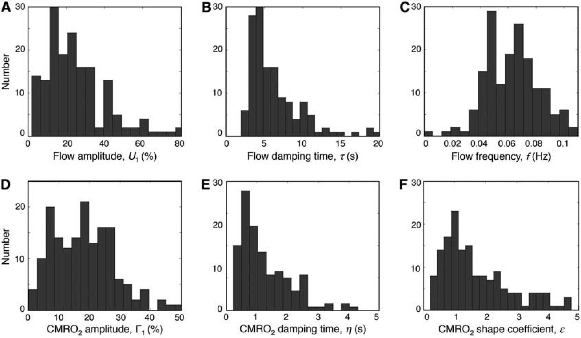
Histograms for six optimization parameters. Three cerebral blood flow parameters are shown in upper panels. (
We repeated the fitting procedure using six different sets of steady-state parameters, adjusting the initial transmural gradient (à), steady-state CMRO2 (Γ ss ) and CBF (Uss) between the endpoints of the ranges described in the Materials and Methods (Table 2). The changes in the steady state produce interesting changes in the two responseamplitude fitting parameters. Increasing the steady-state CMRO2 from 0.01 to 0.05 μmol/L/s causes the CBF response amplitude to decrease from 34.3% to 23.1% with little change in the CMRO2 response amplitude, 22% to 18%. Increasing Γ ss also affects the shape of both responses, with CBF frequency decreasing by 18.5% and CMRO2 shape coefficient e increasing from 1.2 to 2.3. Thus, as steady-state metabolism increases, both flow and CMRO2 responses occur more slowly. In contrast, as the transmural gradient is increased from 0.1 to 0.3, the CMRO2 response amplitude decreases from 19.7% to 9.7%, without change in the CBF response. Changing the transmural gradient has a nearly linear effect on only the CMRO2 response amplitude, with little change to its time course. Increasing Uss from 0.61 to 5.52 μm/s causes a decrease in both CBF and CMRO2 response amplitudes from 40.2% to 21.6%, and 17.0% to 12.3%, respectively. This change is non-linear, mostly occurring as Uss increases from the low to intermediate flow speeds. It is notable that as all three steady-state parameters are increased over these ranges, the variance in the CMRO2 response decreases by a factor of ~2. In all cases, our model successfully fit >95% of the experimental measurements.
Means and standard deviations of optimization parameters for fits to the same experimental data using 7 different sets of steady-state parameters

For successful fits, we examine correlations between the observed neuronal activity and the optimization parameters. We find strong and significant correlation (R = 0.40, P<0.0001) between the neuronal activity and the CMRO2 response amplitude (Figure 7A). On the contrary, there is a mild negative correlation R = −0.18, P~0.02) between neuronal activity and the flow response amplitude (Figure 7B). A mild correlation (R = 0.23, P~0.003) is also found for the flow damping time (Figure 7C). The other three parameters show insignificant correlations with neuronal activity.
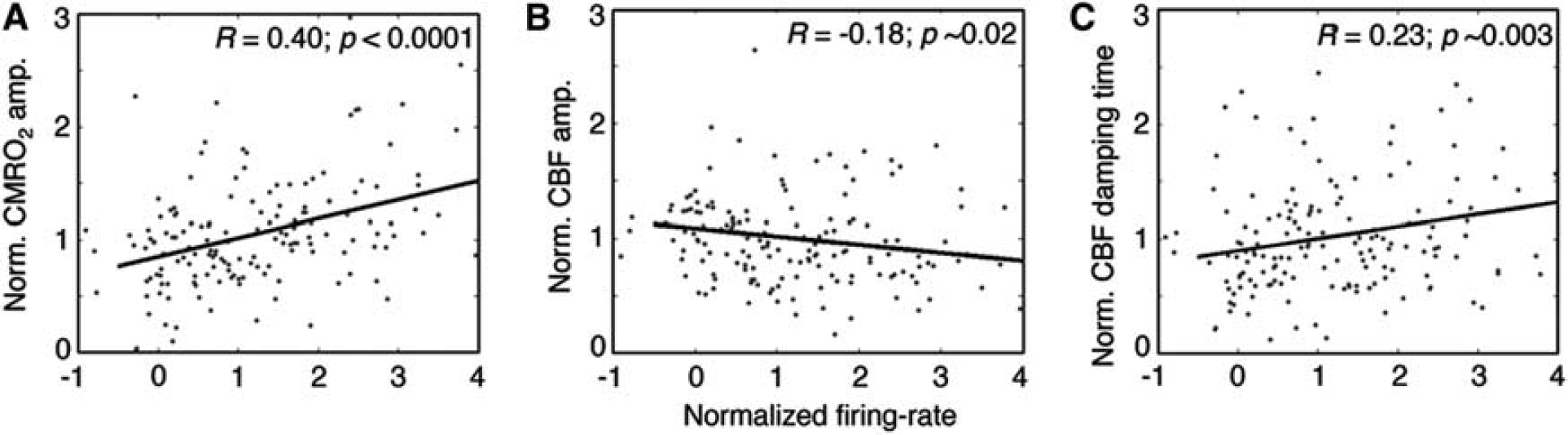
Correlations between optimization parameters and neuronal activity. (
DISCUSSION
We provide a novel model based upon 1D convection-diffusion oxygen transport in a cylindrical three-compartment geometry. It accurately accounts for hemoglobin dissociation (neglected in previous efforts3,11,12,16), which allows predictions of absolute oxygen concentrations both in steady state and during the response to brief neural stimulation. Neural activity is assumed to produce responses in CBF and CMRO2 based on linear models, and these responses compete with each other to predict measured extravascular oxygen concentrations. Thus, the model provides a detailed physiologic interpretation of neurovascular and neurometabolic coupling in the brain. Accurate fits to experimental data are possible starting from a wide range of plausible steady states, and the model permits testing of a wall-consumption hypothesis.
The proximal-integration hypothesis motivates use of a lumped linear flow model, a FEW. This flow impulse response has the form of a damped harmonic oscillator. Previous models used oscillatory descriptions to model the flow response.28,29 Here, we provide a physiologic basis for this oscillatory character in terms of energy exchange between the kinetic energy of moving arterial blood, and energy stored in the compliance of the downstream venous vasculature.
The oscillatory character of this flow model permits fits to the undershoot and ringing observed in our measured extravascular oxygen time courses. The flow frequency has a bimodal distribution at ~0.05 and ~0.07 Hz. The modeled frequencies are ~0.05 Hz lower than the spectral centroids of the raw experimental data suggesting non-linear coupling between the CBF and CMRO2 responses. The observed ringing is also consistent with underdamped flow responses measured using optical imaging spectroscopy, 36 two-photon imaging, 4 and laser speckle. 37 Moreover, we find a mild correlation between neural activity and flow-damping time (Figure 7C). Greater neuronal activity generates greater oxygen demand in the neuropil, and the observed increase in ringing may reflect a decrease in damping time that speeds the delivery of oxygenated blood to the activated tissue.
However, most experiments in rodents do not show strong ringing. This could be a consequence of anesthesia, which strongly dampens the HRF.36,38 Also, we show here that stimulus-evoked ringing has substantial site-to-site variations in frequency, so the ringing would be masked to spatially averaged measurements such as laser speckle or Doppler flowmetry.31,39 Regardless, our model is also capable of fitting non-oscillatory flow responses using the overdamped form of the FEW impulse response.
Low-frequency fluctuations have been observed extensively in the cerebrovasculature and are sometimes termed Mayer waves, which exhibit several frequency bands.40,41 Our predicted flow fluctuations are in good correspondence to the LF (low frequency) and VLF (very low frequency) bands. Mayer waves in these bands are usually associated with vasomotion, rhythmic fluctuations in vascular tone caused by intravascular calcium variations. 42 Our results suggest that such slow hemodynamic oscillations can be driven indirectly by neural activity in the parenchyma by way of the proximal-integration response. In this view, neural activity would generate local vasodilation, leading to mechanical fluid shear that drives waves of vascular tone changes, a phenomenon similar to vasomotion in the brain.
The stimulus-evoked CBF response amplitudes are consistent with experimental measurements. Mean CBF response amplitude is 25.4%, which is similar to experimental measurements (~30%) by PET and functional magnetic resonance imaging (fMRI). 43 However, there is no positive correlation between neuronal activity and CBF response amplitude (Figure 7B). This suggests that the flow response is not tightly localized, but occurs on a coarser spatial scale than the localized neuronal activity, which in these experiments varies on the 0.7-mm scale of the feline ocular dominance columns. A less localized flow response is consistent with the proximal-integration hypothesis, which suggests that local neural activity gives rise to an upstream vascular response that spreads in spatial extent.
The predicted activity-induced increase in CMRO2 has a mean value, ~19%, which is similar to values (~10%) measured using PET 44 and fMRI. 45 We find a strong correlation between neuronal activity and CMRO2-response amplitude (Figure 7A), consistent with the assertion that neuronal activity gives rise to localized oxygen demand in the tissue. 17
We simulate CMRO2 responses using a gamma function. Measurements of oxygen consumption by brief neuronal activation have demonstrated relatively fast increases and slow decays, 32 which we can model using appropriate choices for shape coefficient and time constant. The prompt increase in CMRO2 directly causes the initial dip in extravascular oxygen measurements. In all cases, the CMRO2 response begins first, followed by the CBF response, consistent with immediate consumption of oxygen by the neuropil due to the transient neural activity. This initially leads to a drop of oxygen in the tissue that is only slowly remediated by the sluggish CBF response. Later, the continued competition between the CMRO2 response and the oscillatory CBF response determines how the extravascular oxygen concentration returns to steady state, thus describing the observed heterogeneous late-time responses.
The model provides an analytic solution for the cerebrovascular steady state, which allows interesting predictions. We are particularly interested in the effects of oxygen consumption by the blood-vessel wall (or apposed tissues) on steady-state mass balance. We chose a small transmural gradient consistent with previous polarographic measurement in cerebral cortex,8,18 which corresponds to a relatively small wall consumption (19% of total oxygen consumption). However, wall consumption can contribute up to ~90% of oxygen consumption, depending upon the choice of transmural gradient and steady-state CMRO2 (Figures 4A and 4D). Additional experiments that measure absolute oxygen concentrations will be needed to determine how much wall consumption is actually present.
The steady-state solution also determines the length of the simulated blood vessel, which provides a rough estimate of where oxygen transport occurs in the parenchyma. Our steady-state model predicts a range of cylinder lengths, 26 to 1,017 μm, depending upon parameter choices. Shorter lengths are consistent with oxygen delivery from capillaries (<200 μm), while longer lengths suggest delivery from arterioles and capillaries (~900 μm). The model is thus consistent with previous experimental oxygen-transport findings.8,10,19
We investigated the effect of transmural gradient, steady-state CBF, and CMRO2 on the optimization parameters. The changes modify the balance between CBF and CMRO2 responses, but both remain in a physiologically reasonable range, and excellent fits to our experimental measurements are still obtained. Further experiments, therefore, will be necessary to elucidate the appropriate choices for the steady state.
Our model can be broadly used to interpret and predict oxygen transport in the brain. For example, the model can be applied to localized measurements of CBF as well as intra- and extravascular oxygen concentrations that are now becoming available using two-photon imaging methods.46–48 From these measurements, the model can provide estimates of temporal CMRO2 responses. Moreover, the model can also predict blood oxygen-level dependent (BOLD) fMRI responses. Recent experiments suggest that there is no significant venous blood volume change for vascular and metabolic responses evoked by brief neural stimulation.4,5,32 Therefore, the BOLD response is primarily a function of the intravascular oxygen concentration and can be estimated by our model (Appendix 3). Further brief-stimulation experiments with high-resolution fMRI that are fully localized to the gray matter will be needed to test this new BOLD response model. For such measurements, our model will be able to separate the effects of CBF and CMRO2 on the BOLD HRF.
The model has some limitations. Although we use weighted parameters to consider the volume effect of different vessel sizes, we underestimate the surface-area-to-volume ratio by representing the vastly branching capillary bed by a single cylinder. We can remediate this flaw by using a parallel network that breaks the effective blood volume into many identical branches. Including a longitudinal series of compartments to represent multiple orders of arterioles and the capillary bed would also increase the accuracy of the model.
This model for the HRF does not attempt to explain the mechanisms of longer neural stimulation that do lead to microvascular venous volume changes. Previous models that postulate venous inflation are motivated by the slow hemodynamic responses of oxygen autoregulation.3,11,12,49,50 Such mechanisms are likely essential to describe the hemodynamic response to extended periods of neural activity (tens of seconds). We believe that both the transient mechanisms described by our model, and the slower mechanisms that yield venous dilation are likely to operate in parallel, and both hemodynamic response mechanisms must be included depending upon time scale.
To interpret the experimental data from a polarographic oxygen sensor, we had to make a spatial sampling assumption. Because oxygen transport mainly occurs in capillaries (~52% of total oxygen transport),8,18 we chose to use the predicted extravascular oxygen concentration over a 60-mm region at the distal end of the model blood vessel, which corresponds to the mean length of a capillary segment. 34 However, we also tested two other sampling approaches: permitting the sampling to vary along the length of the cylinder as an optimization parameter, and averaging over the entire blood-vessel length. These approaches also provide good fits to the measurements that were qualitatively identical to those presented in the Results.
In conclusion, our computational model uses a simple geometry and tractable computations to provide accurate and detailed predictions of transient oxygen responses with heterogeneous combinations of initial dips, hyperoxic peaks, undershoots, and ringing in cat visual cortex using only six optimization parameters. The FEW flow model provides a mechanism by which neural activity couples to parenchymal CBF in a substantially linear fashion. The model is flexible, as overdamped flow responses could also fit experimental data that do not show ringing. The realistic steady-state formulation is adjustable, permitting tests of hypotheses for oxygen transport mechanisms. Altogether, the model provides a theoretical framework to explain the full panoply of vascular and metabolic responses evoked by brief neural stimulation in the gray matter of the brain.
DISCLOSURE/CONFLICT OF INTEREST
The authors declare no conflict of interest.
Footnotes
ACKNOWLEDGEMENTS
The authors thank Ralph Freeman for providing the experimental data, and Rick Buxton for providing thoughtful comments and advice.
APPENDIX 1
APPENDIX 2
APPENDIX 3
References
Supplementary Material
Please find the following supplemental material available below.
For Open Access articles published under a Creative Commons License, all supplemental material carries the same license as the article it is associated with.
For non-Open Access articles published, all supplemental material carries a non-exclusive license, and permission requests for re-use of supplemental material or any part of supplemental material shall be sent directly to the copyright owner as specified in the copyright notice associated with the article.