Additive manufacturing technology is gaining significant attention in many industries such as automobile, aerospace, and medical. In particular, directed-energy additive manufacturing using a laser source is of central interest, thanks to its geometric precision and higher quality products compared with other heat sources. To produce high-quality components, in-situ melt pool monitoring technology is required. This article deals with an in-situ melt pool size estimation method for directed-energy additive manufacturing using the measured resonant frequency and damping ratio. The test set-up is composed of an impact hammer and two laser Doppler vibrometers (LDV) connected to a Siemens LMS SCADAS FFT analyzer. The LDV was used to measure the velocity of the melt pool and an Al beam, whereas the impulse signal is given by the impact hammer. The melt pool shape was machined by drilling into the top surface of an Al beam that is 50 mm wide and 100 mm long. The diameter (D) of the melt pool was machined to 1 and 2 mm, and the depth of melt pool was machined from 0.5 to 1.5 D. A low-melting-temperature metal that transitions a 70°C was used to readily achieve the liquid state of the melt pool in a laboratory environment. The frequency response function results were obtained from the Siemens Test Laboratory Software. Then the modal parameters were calculated by using the rational fraction polynomial method to extract the natural frequency and damping ratio according to the Al beam length, melt pool diameter, and melt pool depth. As a result, we confirmed that the difference in the resonant frequency and a damping ratio of the melt pool was a function of the Al beam length, melt pool diameter, and melt pool depth.
Introduction
Additive manufacturing, first demonstrated in 1981 by “printing” a polymeric solid using individual layers, has quickly become a dominant player for producing high-quality, complex, and individually customized parts. The additive manufacturing techniques were originally developed for engineering prototype production. These technologies are currently applied in numerous fields, such as aerospace, automotive, mechanical engineering, and medicine.1–4
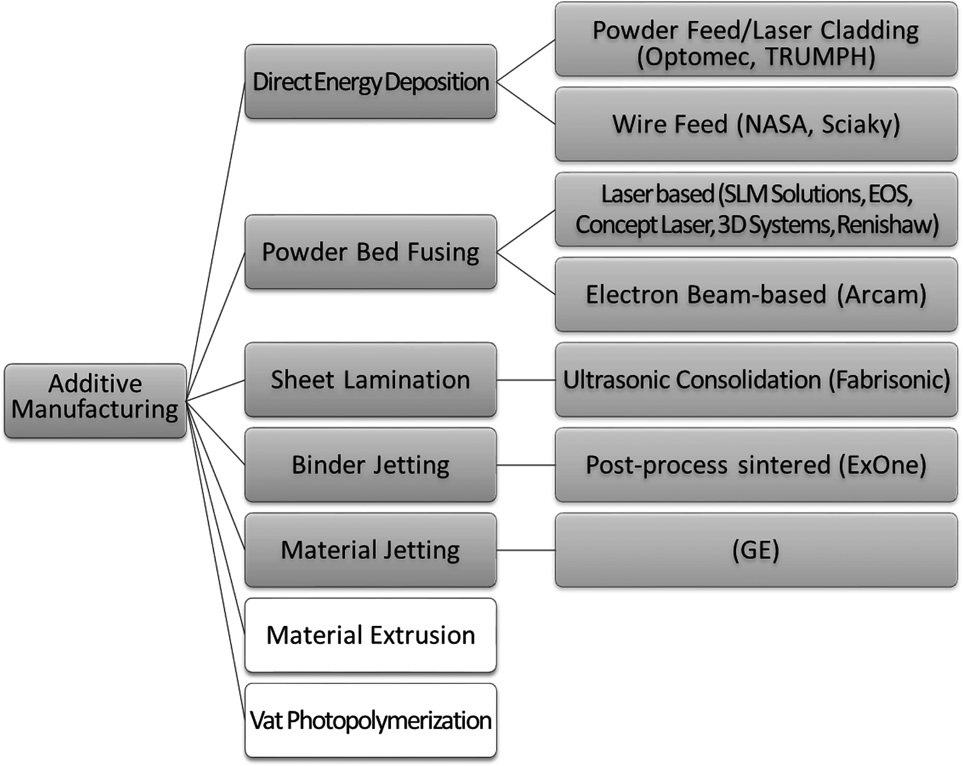
Additive manufacturing can be performed using various materials, such as polymers, metals, ceramics, and composites. Figure 1 shows representative metal and nonmetal additive manufacturing processes grouped by type using the terminology of ASTM F2792.5 The processes in the blue boxes are applicable to metals, and the processes in the white boxes are applicable to polymer-based materials only.
Representative additive manufacturing processes grouped by type using the terminology of ASTM F2792.1
Most additive manufacturing processes, especially using metal, include generation of a melt pool. The size and shape of this melt pool strongly affects the texture, crystal structure, and residual stress of the final part. Some final parts can be inspected by X-ray6 or computed tomography7 to ensure the quality of final part. However, these methods have limitations in terms of part size and the safety. In addition, off-line inspection system cannot detect defects during the manufacturing process.
The sources of defects during the additive manufacturing process can be classified into two categories: equipment-induced errors and process-induced errors. These errors are important factors when geometric accuracy cannot be improved through postprocessing. Due to these reasons, many researchers have developed various in-situ monitoring systems to check for errors during manufacturing.
Nondestructive testing for in-situ monitoring system of additive manufacturing has been developed using several techniques, such as optical emission spectroscopy (OES), laser ultrasonic, and optical coherence tomography (OCT). OES for monitoring of additive manufacturing processes was investigated by several research groups.8–11 The OES technique has been used to understand physical mechanisms and to monitor conditions of melt pool during the additive manufacturing. Bartkowiak et al.8 and by Song et al.9,10 successfully demonstrated the potential utility of OES for monitoring of additive manufacturing processes. The use of scanning laser transmitter and receiver and the interaction of the incident ultrasonic wave with subsurface and surface defects have been widely investigated.12,13 A laser ultrasonic technique for the additive manufacturing of laser metal deposition (LMD) has been suggested by Cerniglia et al.14 The use of a laser ultrasonic technique to detect defects in LMD components has been assessed to inspect and perform quality control during manufacturing. They successfully detected the defects with size from 100 μm and depth up to 700 μm with high sensitivity. An optical coherence technique for the additive manufacturing (AM) of selective laser sintering (SLS) has been suggested by Guan et al.15 Their study has demonstrated the feasibility of using OCT for investigation the surface topography and subsurface structure of polymeric parts manufactured using SLS. The OCT could present a viable route to real-time, in-situ process monitoring, and control during SLS process. They successfully demonstrated the detection of defects smaller than 9 μm. Rangaswamy et al. suggested the observation method, which comes from direct thermal imaging of the melt pool during metal deposition.16 However, the existing techniques for the melt pool monitoring measured the surface geometry, such as width and length, but not depth.
This article focuses on the estimation of melt pool size using modal parameters, such as natural frequency and damping ratio, because these parameters are a function of the state of melt pool and host structure. For example, the natural frequency or damping ratio should vary according to the melt pool size due to its dimensional change. Therefore, we can estimate the melt pool size if we can measure the frequency response function (FRF) of the melt pool precisely. For this, two laser Doppler vibrometers (LDV) were used to measure the velocities of the melt pool and the host structure, respectively, when applying an impulsive signal using an impact hammer. The rational fraction polynomial method17 was used to estimate the natural frequency, and damping ratio is calculated using the Q factor obtained from the FRF results. The AM product changes size, shape, and weight during the manufacturing process, so we first provided an impulse to the structure with wideband frequency excitation to measure its modal parameters. Once the natural frequency is determined, monitoring is carried out using steady-state excitation at that frequency. Melt pool monitoring using steady-state excitation and laser ultrasound detection provides three significant benefits: (1) Excitation energy is effectively transmitted into the melt pool structure; (2) Measurement time can be reduced; and (3) Melt pool depth can be estimated in real-time.
Experimental Set-Up
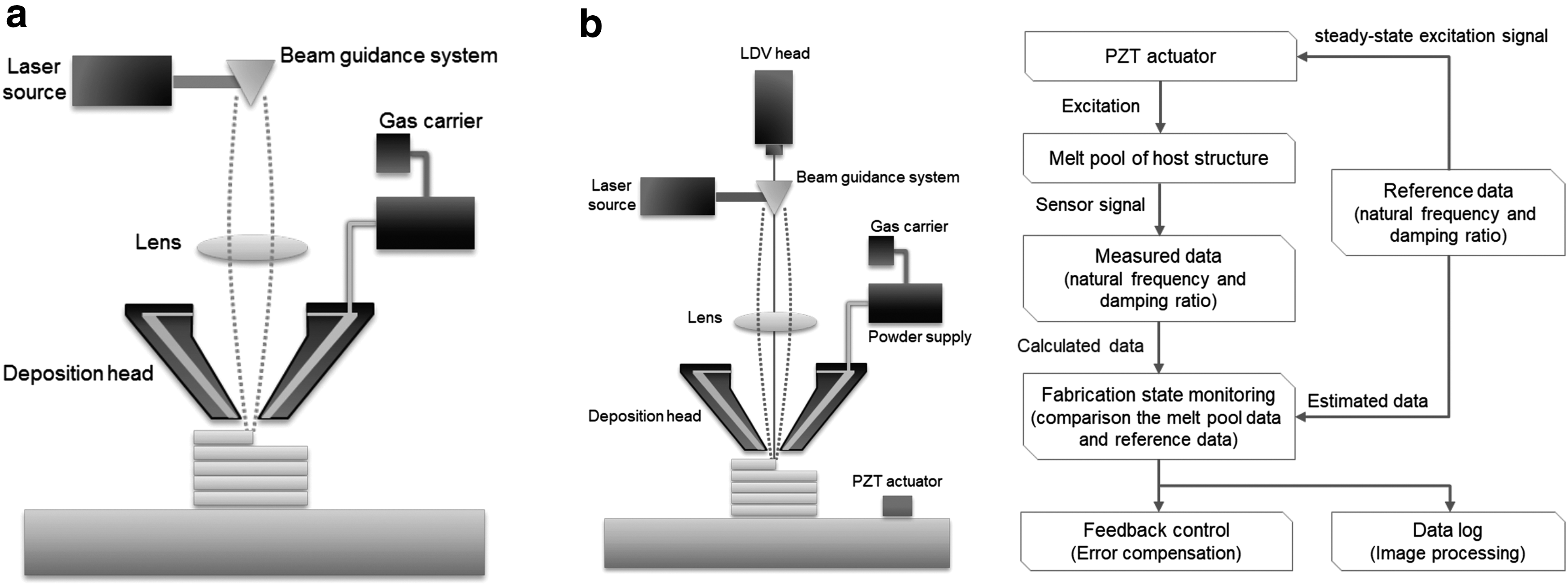
In directed-energy deposition (DED) material is deposited using the focused energy, such as from an electron beam or the laser beam.18,19 DED systems can be classified into two groups according to the feedstock: powder feed, such as LMD, and wire feed. The DED process is evolved out of the laser welding and laser cladding technologies. The major components of the DED system are the energy source, material feeding system, and the deposition head mounted on a multi-axis arm. The DED process is similar to material extrusion, however, the deposition head of the DED system can move to multiple directions according to the installed multi-axis arm. The powder-based system illustrated in Figure 2a operates by jetting the powder on the surface using carrier gas such as argon gas. This argon gas also provides the surface shielding to prevent oxide formation on the deposition layer during the process.
Schematics of the powder-based directed-energy deposition: (a) A representative of the DED methods; (b) A suggested DED with in-situ monitoring system and melt pool size estimation algorithm. DED, directed-energy deposition; LDV, laser Doppler vibrometers; PZT, lead zirconate titanate (Pb(Zr,Ti)O3).
Figure 2b shows the suggested concept of the DED system with in-situ melt pool size monitoring prototype. The LDV was installed on the existing DED system to estimate the melt pool size during the manufacturing process, and the lead zirconate titanate (Pb(Zr,Ti)O3) actuator is also installed on the base plate to excite the deposited structure at the steady-state frequency of the host structure that is calculated using FEM.
Specimen geometry for the melt pool shapes
Melt pool geometry is highly dependent on laser beam power or fabrication speed in the cases of electron beam or laser beam additive manufacturing process. The melt pool geometry varies very noticeably; for example, in the case of using a 360 W source power, the melt pool length varies from 40 \documentclass{aastex}\usepackage{amsbsy}\usepackage{amsfonts}\usepackage{amssymb}\usepackage{bm}\usepackage{mathrsfs}\usepackage{pifont}\usepackage{stmaryrd}\usepackage{textcomp}\usepackage{portland, xspace}\usepackage{amsmath, amsxtra}\usepackage{upgreek}\pagestyle{empty}\DeclareMathSizes{10}{9}{7}{6}\begin{document}
$${ \rm{ \mu m}}$$
\end{document} to about 1750 \documentclass{aastex}\usepackage{amsbsy}\usepackage{amsfonts}\usepackage{amssymb}\usepackage{bm}\usepackage{mathrsfs}\usepackage{pifont}\usepackage{stmaryrd}\usepackage{textcomp}\usepackage{portland, xspace}\usepackage{amsmath, amsxtra}\usepackage{upgreek}\pagestyle{empty}\DeclareMathSizes{10}{9}{7}{6}\begin{document}
$${ \rm{ \mu m}}$$
\end{document}; its width varies from 26 \documentclass{aastex}\usepackage{amsbsy}\usepackage{amsfonts}\usepackage{amssymb}\usepackage{bm}\usepackage{mathrsfs}\usepackage{pifont}\usepackage{stmaryrd}\usepackage{textcomp}\usepackage{portland, xspace}\usepackage{amsmath, amsxtra}\usepackage{upgreek}\pagestyle{empty}\DeclareMathSizes{10}{9}{7}{6}\begin{document}
$${ \rm{ \mu m}}$$
\end{document} to about 870 \documentclass{aastex}\usepackage{amsbsy}\usepackage{amsfonts}\usepackage{amssymb}\usepackage{bm}\usepackage{mathrsfs}\usepackage{pifont}\usepackage{stmaryrd}\usepackage{textcomp}\usepackage{portland, xspace}\usepackage{amsmath, amsxtra}\usepackage{upgreek}\pagestyle{empty}\DeclareMathSizes{10}{9}{7}{6}\begin{document}
$${ \rm{ \mu m}}$$
\end{document}; and its depth varies from 2.5 \documentclass{aastex}\usepackage{amsbsy}\usepackage{amsfonts}\usepackage{amssymb}\usepackage{bm}\usepackage{mathrsfs}\usepackage{pifont}\usepackage{stmaryrd}\usepackage{textcomp}\usepackage{portland, xspace}\usepackage{amsmath, amsxtra}\usepackage{upgreek}\pagestyle{empty}\DeclareMathSizes{10}{9}{7}{6}\begin{document}
$${ \rm{ \mu m}}$$
\end{document} to 326 \documentclass{aastex}\usepackage{amsbsy}\usepackage{amsfonts}\usepackage{amssymb}\usepackage{bm}\usepackage{mathrsfs}\usepackage{pifont}\usepackage{stmaryrd}\usepackage{textcomp}\usepackage{portland, xspace}\usepackage{amsmath, amsxtra}\usepackage{upgreek}\pagestyle{empty}\DeclareMathSizes{10}{9}{7}{6}\begin{document}
$${ \rm{ \mu m}}$$
\end{document}.20 In the case of using over 1000 W source power, the melt pool depth is around 5 mm; and melt pool width is around 10 mm.21
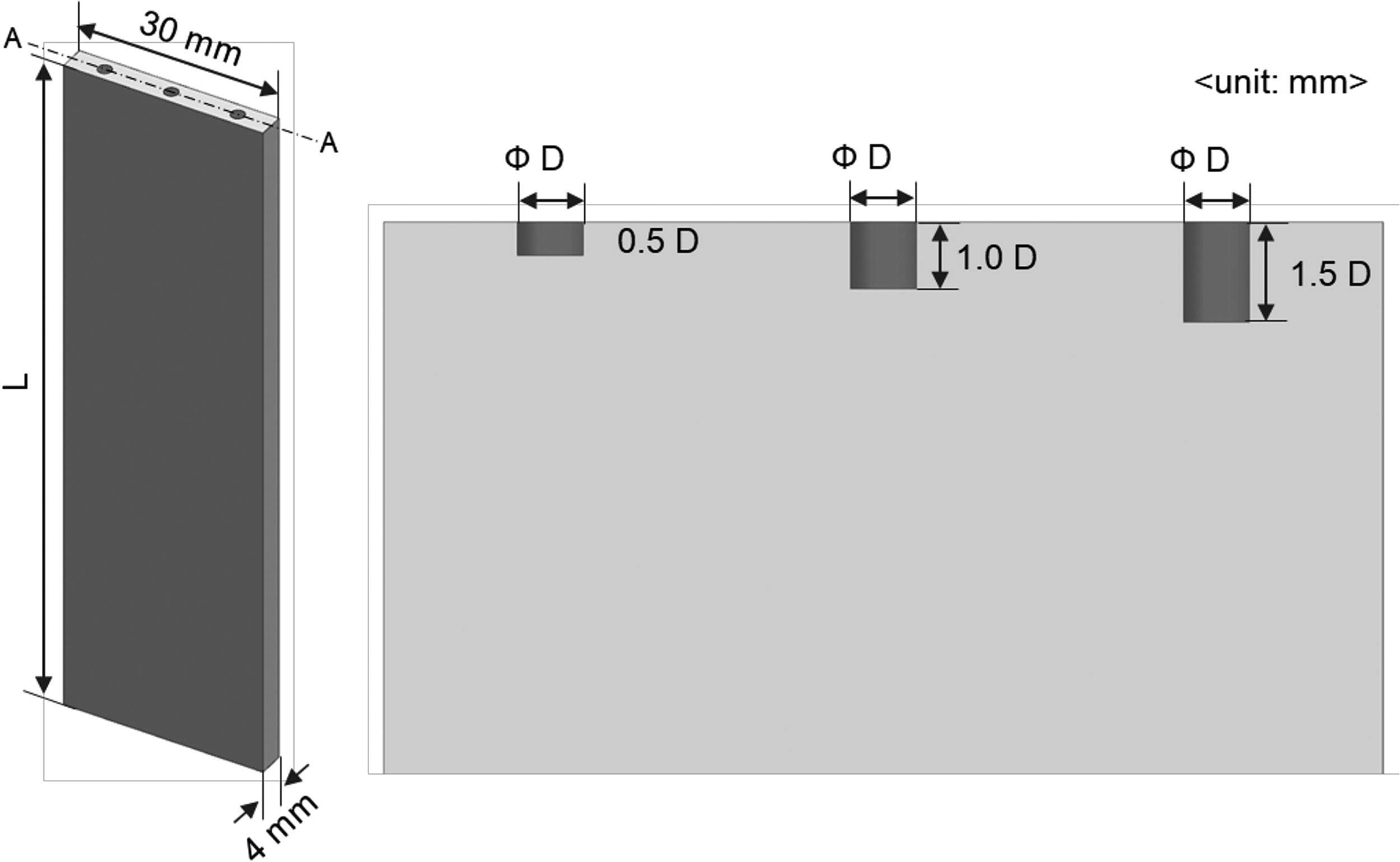
To check the effect of the melt pool size and aluminum beam length on the natural frequency and damping ratio, we prepared four validation specimens as illustrated in Figure 3. The dimensions of the melt pool and Al beam are summarized in Table 1. The host structure is an Al beam with a width of 30 mm, a thickness of 4 mm, and a height of 50 and 100 mm. The depth of melt pool of low-melting-temperature metal (3-110-980; Kenis, Inc.) was controlled from 0.5 to 1.5 D. The diameter of the melt pool was set to 1 and 2 mm. The Al beam's first natural frequency was calculated using the ANSYS modal analysis module.
Specimen geometry for the melt pool shapes and Al beam.
Geometrical Dimensions of Al Beam with Melt Pool Shape (Unit: mm)
Geometrical dimensions
Al beam
Melt pool
Thickness (T)
Width (W)
Height (H)
Diameter (D)
Depth (d)
No. 1
4
30
50
1
0.5 D 1.0 D 1.5 D
No. 2
2
No. 3
100
1
No. 4
2
In this study, the melt pool shape was simulated by drilling on the top surface of the Al beam using end-mill drill tip. The low-melting-temperature metal, which melts at 70°C, was utilized so that experiments could be conducted without an environmental chamber and without modifying a DED system. The material properties of the Al beam and low-melting-temperature metal are summarized in Table 2.
Material Properties of the Al Beam and Low Melting Temperature Metal
Material properties
Density (kg/m3)
Young's modulus (GPa)
Poisson's ratio
Melting point (°C)
Al beam
2700
68.9
0.33
582
LMTM
4200
—
—
70
LMTM, low melting temperature metal.
Melt pool depth-monitoring test set-up
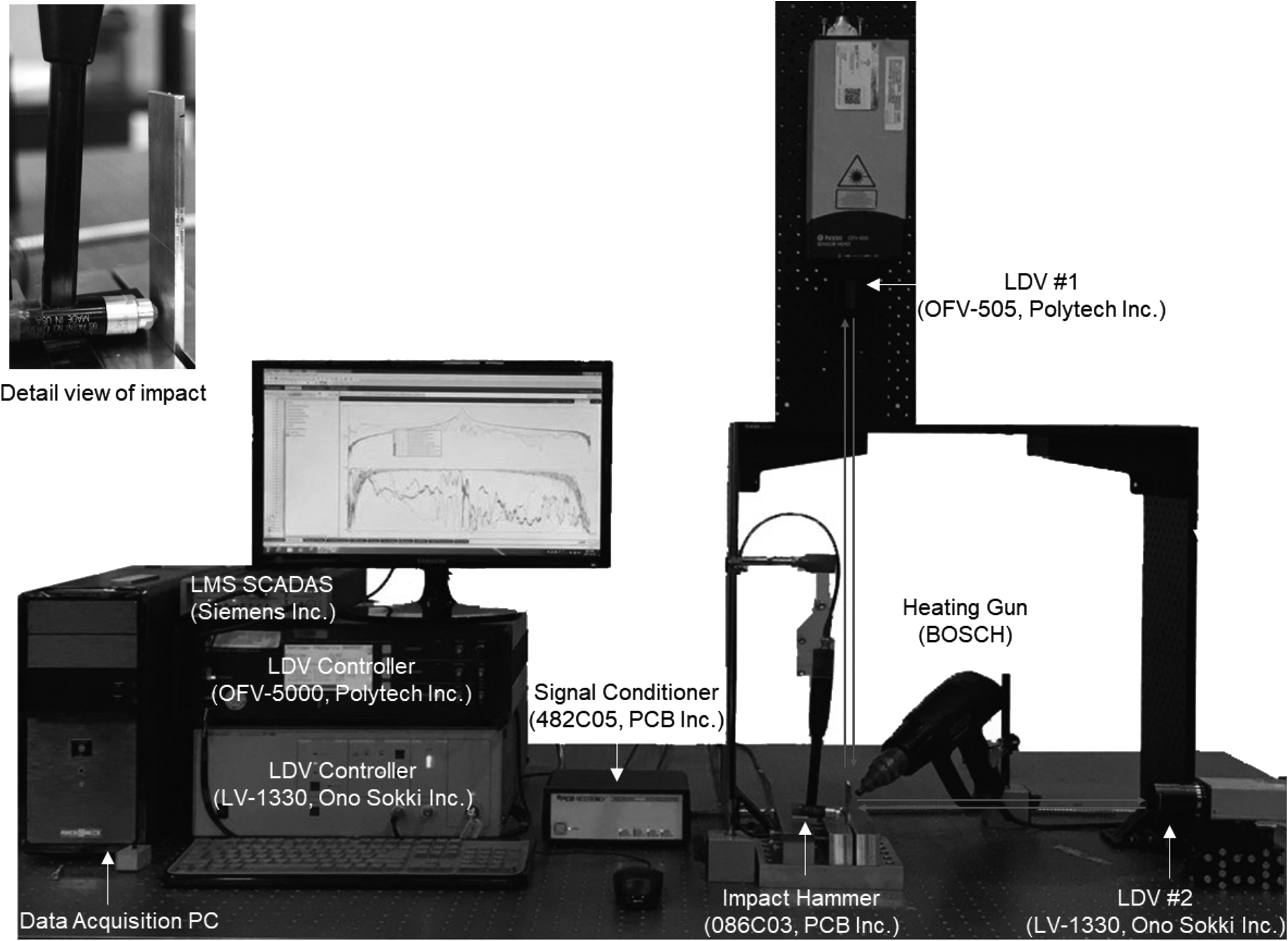
The melt pool size estimation test concept is illustrated in Figure 4, and the actual test set-up is shown in Figure 5. Two LDV systems were employed. The first one (LV-1330; Ono Sokki, Inc.) measures the velocity of the Al beam, and the second (OFV-505 and OFV-5000; Polytech, Inc.) measures the velocity of the melt pool surface when the Al beam was excited by impact hammer (086C03, PCB, Inc.; 482C05, PCB, Inc.). The signals from the LDV systems and impact hammer are passed through a signal conditioner and captured with a DAQ device (LMS SCADAS; Siemens, Inc.), and then the FRF was computed using commercial modal software (LMS Test Lab.; Siemens, Inc.) to check the natural frequency of the melt pool and the Al beam according to the melt pool depth. Also, the heating gun (GHG 636; BOSCH, Inc.) was installed to achieve the liquid state melt pool. The specifications and settings of the devices are summarized in Table 3. The velocity value of the LDV for measuring the melt pool is 100 mm/s/V with the low-pass filter set at 10 kHz. The velocity value of the LDV for measuring the Al beam is 100 mm/s/V with the low-pass filter set at 10 kHz. The sensitivity of the impact hammer is 11.72 mV/N. The sensor voltage signals were converted to their original physical units to compute the FRF in the LMS Test Laboratory. The heating gun temperature was fixed at 200°C by considering the heat loss. The temperature of the melt pool was 81.6°C, when we measured the melt pool surface using a noncontact IR thermometer.
Schematic test set-up for the melt pool size estimation using the LDV.
Actual test set-up for the melt pool size estimation using the LDV.
Laser Doppler Vibrometer Setting Values for the Measurement
Device setting value
Velocity value (mm/s/V)
High-pass filter (kHz)
Low-pass filter (kHz)
LV-1330
100
—
10
OFV-5000
100
—
10
Experimental Results
In this study, we assumed that the natural frequency or damping ratio can be changed based on the surface condition: For example, the FRF can be very sharp when measuring on the hard surface of the host plate, but the FRF can be smoother when measuring on the soft surface like melt pool. Furthermore, the frequency and damping ratio can also be changed according to the melt pool depth. If the FRF signals are successfully measured by using two LDV systems under the impulse excitation condition, we can check the difference of the natural frequency and damping ratio from the damped natural frequencies, calculated by the following Eqs. (1)–(4).
The excitation signal from the impact hammer and the consequent structural responses measured using LDV sensors were captured, and the FRF was computed in the LMS Test Laboratory module. The FRF is most commonly used for single input and single output to analyze the characteristic of the system.22 The FRF is defined as the ratio of the complex spectrum of the response to the complex spectrum of the excitation as described in Eq. (1),
\documentclass{aastex}\usepackage{amsbsy}\usepackage{amsfonts}\usepackage{amssymb}\usepackage{bm}\usepackage{mathrsfs}\usepackage{pifont}\usepackage{stmaryrd}\usepackage{textcomp}\usepackage{portland, xspace}\usepackage{amsmath, amsxtra}\usepackage{upgreek}\pagestyle{empty}\DeclareMathSizes{10}{9}{7}{6}\begin{document}
\begin{align*}
H \left( f \right) = { \frac { Y \left( f \right) } { X \left( f \right) } } \tag { 1 }
\end{align*}
\end{document}
where, \documentclass{aastex}\usepackage{amsbsy}\usepackage{amsfonts}\usepackage{amssymb}\usepackage{bm}\usepackage{mathrsfs}\usepackage{pifont}\usepackage{stmaryrd}\usepackage{textcomp}\usepackage{portland, xspace}\usepackage{amsmath, amsxtra}\usepackage{upgreek}\pagestyle{empty}\DeclareMathSizes{10}{9}{7}{6}\begin{document}
$$H \left( f \right)$$
\end{document} is the FRF, \documentclass{aastex}\usepackage{amsbsy}\usepackage{amsfonts}\usepackage{amssymb}\usepackage{bm}\usepackage{mathrsfs}\usepackage{pifont}\usepackage{stmaryrd}\usepackage{textcomp}\usepackage{portland, xspace}\usepackage{amsmath, amsxtra}\usepackage{upgreek}\pagestyle{empty}\DeclareMathSizes{10}{9}{7}{6}\begin{document}
$$Y \left( f \right)$$
\end{document} is the output from the system in the frequency domain, and \documentclass{aastex}\usepackage{amsbsy}\usepackage{amsfonts}\usepackage{amssymb}\usepackage{bm}\usepackage{mathrsfs}\usepackage{pifont}\usepackage{stmaryrd}\usepackage{textcomp}\usepackage{portland, xspace}\usepackage{amsmath, amsxtra}\usepackage{upgreek}\pagestyle{empty}\DeclareMathSizes{10}{9}{7}{6}\begin{document}
$$X \left( f \right)$$
\end{document} is the input to the system in the frequency domain. \documentclass{aastex}\usepackage{amsbsy}\usepackage{amsfonts}\usepackage{amssymb}\usepackage{bm}\usepackage{mathrsfs}\usepackage{pifont}\usepackage{stmaryrd}\usepackage{textcomp}\usepackage{portland, xspace}\usepackage{amsmath, amsxtra}\usepackage{upgreek}\pagestyle{empty}\DeclareMathSizes{10}{9}{7}{6}\begin{document}
$$H{ \left( f \right) _{melt \;pool}}$$
\end{document} is the ratio of the melt pool response [\documentclass{aastex}\usepackage{amsbsy}\usepackage{amsfonts}\usepackage{amssymb}\usepackage{bm}\usepackage{mathrsfs}\usepackage{pifont}\usepackage{stmaryrd}\usepackage{textcomp}\usepackage{portland, xspace}\usepackage{amsmath, amsxtra}\usepackage{upgreek}\pagestyle{empty}\DeclareMathSizes{10}{9}{7}{6}\begin{document}
$$Y{ \left( f \right) _{melt \;pool}}$$
\end{document}] to the impact hammer [\documentclass{aastex}\usepackage{amsbsy}\usepackage{amsfonts}\usepackage{amssymb}\usepackage{bm}\usepackage{mathrsfs}\usepackage{pifont}\usepackage{stmaryrd}\usepackage{textcomp}\usepackage{portland, xspace}\usepackage{amsmath, amsxtra}\usepackage{upgreek}\pagestyle{empty}\DeclareMathSizes{10}{9}{7}{6}\begin{document}
$$X{ \left( f \right) _{Impact}}$$
\end{document}] and [\documentclass{aastex}\usepackage{amsbsy}\usepackage{amsfonts}\usepackage{amssymb}\usepackage{bm}\usepackage{mathrsfs}\usepackage{pifont}\usepackage{stmaryrd}\usepackage{textcomp}\usepackage{portland, xspace}\usepackage{amsmath, amsxtra}\usepackage{upgreek}\pagestyle{empty}\DeclareMathSizes{10}{9}{7}{6}\begin{document}
$$H{ \left( f \right) _{Al \;beam}}$$
\end{document}] is the ratio of the Al beam response [\documentclass{aastex}\usepackage{amsbsy}\usepackage{amsfonts}\usepackage{amssymb}\usepackage{bm}\usepackage{mathrsfs}\usepackage{pifont}\usepackage{stmaryrd}\usepackage{textcomp}\usepackage{portland, xspace}\usepackage{amsmath, amsxtra}\usepackage{upgreek}\pagestyle{empty}\DeclareMathSizes{10}{9}{7}{6}\begin{document}
$$Y{ \left( f \right) _{Al \;beam}}$$
\end{document}] to the impact hammer [\documentclass{aastex}\usepackage{amsbsy}\usepackage{amsfonts}\usepackage{amssymb}\usepackage{bm}\usepackage{mathrsfs}\usepackage{pifont}\usepackage{stmaryrd}\usepackage{textcomp}\usepackage{portland, xspace}\usepackage{amsmath, amsxtra}\usepackage{upgreek}\pagestyle{empty}\DeclareMathSizes{10}{9}{7}{6}\begin{document}
$$X{ \left( f \right) _{Impact}}$$
\end{document}].
The damping effect was also considered to check the melt pool shape effect on the first natural frequency of the structure. The damping ratio of the DED product can be less than 1 (0 < \documentclass{aastex}\usepackage{amsbsy}\usepackage{amsfonts}\usepackage{amssymb}\usepackage{bm}\usepackage{mathrsfs}\usepackage{pifont}\usepackage{stmaryrd}\usepackage{textcomp}\usepackage{portland, xspace}\usepackage{amsmath, amsxtra}\usepackage{upgreek}\pagestyle{empty}\DeclareMathSizes{10}{9}{7}{6}\begin{document}
$${ \rm{ {\upzeta} }}$$
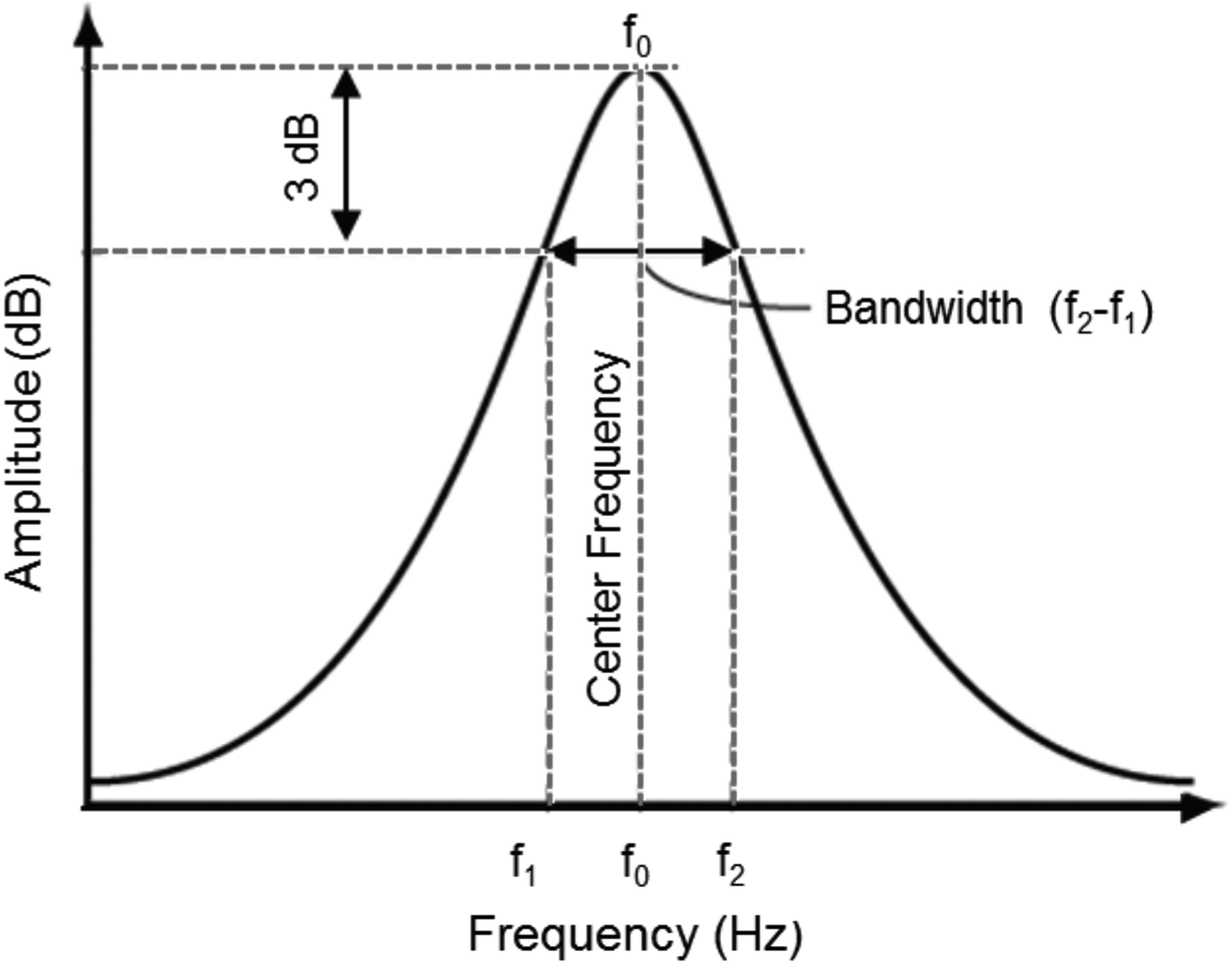
\end{document} < 1), because the DED product can be considered as the underdamped system. This damping ratio can be calculated using the quality factor (Q factor) from the FRF results. The Q factor determines the qualitative behavior of simple damped oscillators: When the Q factor is lower than 0.5, this system is considered to be overdamped; when the Q factor is higher than 0.5, this system is considered to be underdamped; when the Q factor is 0.5, this system is considered to be critically damped. The quality factor (Q) is defined as Eq. (2),
\documentclass{aastex}\usepackage{amsbsy}\usepackage{amsfonts}\usepackage{amssymb}\usepackage{bm}\usepackage{mathrsfs}\usepackage{pifont}\usepackage{stmaryrd}\usepackage{textcomp}\usepackage{portland, xspace}\usepackage{amsmath, amsxtra}\usepackage{upgreek}\pagestyle{empty}\DeclareMathSizes{10}{9}{7}{6}\begin{document}
\begin{align*}
Quality \;Factor \; \left( Q \right) = { \frac { { f_0 } } { \Delta f } } = { \frac { { f_0 } } { { f_2 } - { f_1 } } } \tag { 2 }
\end{align*}
\end{document}
where, the f0 is the natural frequency or center frequency, the \documentclass{aastex}\usepackage{amsbsy}\usepackage{amsfonts}\usepackage{amssymb}\usepackage{bm}\usepackage{mathrsfs}\usepackage{pifont}\usepackage{stmaryrd}\usepackage{textcomp}\usepackage{portland, xspace}\usepackage{amsmath, amsxtra}\usepackage{upgreek}\pagestyle{empty}\DeclareMathSizes{10}{9}{7}{6}\begin{document}
$$\Delta f$$
\end{document} is the half power bandwidth between the f1 and the f2. The f1 is the lower cutoff frequency and the f2 is the upper cutoff frequency as shown in Figure 6. The damping ratio (\documentclass{aastex}\usepackage{amsbsy}\usepackage{amsfonts}\usepackage{amssymb}\usepackage{bm}\usepackage{mathrsfs}\usepackage{pifont}\usepackage{stmaryrd}\usepackage{textcomp}\usepackage{portland, xspace}\usepackage{amsmath, amsxtra}\usepackage{upgreek}\pagestyle{empty}\DeclareMathSizes{10}{9}{7}{6}\begin{document}
$${ \rm{ {\upzeta} }}$$
\end{document}) is defined as Eq. (3),
\documentclass{aastex}\usepackage{amsbsy}\usepackage{amsfonts}\usepackage{amssymb}\usepackage{bm}\usepackage{mathrsfs}\usepackage{pifont}\usepackage{stmaryrd}\usepackage{textcomp}\usepackage{portland, xspace}\usepackage{amsmath, amsxtra}\usepackage{upgreek}\pagestyle{empty}\DeclareMathSizes{10}{9}{7}{6}\begin{document}
\begin{align*}
Damping \;ratio { \rm { \; } } \left( { \rm { { \upzeta } } } \right) = \; \frac { 1 } { { 2 \times Q } } \tag { 3 }
\end{align*}
\end{document}
Definition graph of the quality factor (Q) bandwidth.
In the case of an underdamped system, the damped natural frequency is given by Eq. (4),
\documentclass{aastex}\usepackage{amsbsy}\usepackage{amsfonts}\usepackage{amssymb}\usepackage{bm}\usepackage{mathrsfs}\usepackage{pifont}\usepackage{stmaryrd}\usepackage{textcomp}\usepackage{portland, xspace}\usepackage{amsmath, amsxtra}\usepackage{upgreek}\pagestyle{empty}\DeclareMathSizes{10}{9}{7}{6}\begin{document}
\begin{align*}
{ \omega _d} = { \rm{ \;}}{ \omega _n} \sqrt {1 - { \zeta ^2}} \tag{4}
\end{align*}
\end{document}
where, the \documentclass{aastex}\usepackage{amsbsy}\usepackage{amsfonts}\usepackage{amssymb}\usepackage{bm}\usepackage{mathrsfs}\usepackage{pifont}\usepackage{stmaryrd}\usepackage{textcomp}\usepackage{portland, xspace}\usepackage{amsmath, amsxtra}\usepackage{upgreek}\pagestyle{empty}\DeclareMathSizes{10}{9}{7}{6}\begin{document}
$${ \omega _d}$$
\end{document} is the damped natural frequency and the \documentclass{aastex}\usepackage{amsbsy}\usepackage{amsfonts}\usepackage{amssymb}\usepackage{bm}\usepackage{mathrsfs}\usepackage{pifont}\usepackage{stmaryrd}\usepackage{textcomp}\usepackage{portland, xspace}\usepackage{amsmath, amsxtra}\usepackage{upgreek}\pagestyle{empty}\DeclareMathSizes{10}{9}{7}{6}\begin{document}
$${ \omega _n}$$
\end{document} is the natural frequency.
In the first part of the results and discussion, the melt pool depth effect is explained using the FRF, the damped natural frequency, and damping ratio. Afterward, the melt pool measurement point effect was discussed.
Melt pool diameter (D) and depth effect
This section focuses on the measured natural frequency and damping ratio according to the melt pool diameter and depth. We prepared the No. 3 and No. 4 specimens as summarized in Table 2. The melt pool diameter was set to 1 and 2 mm and the melt pool depth was controlled with 0.5, 1.0, and 1.5 D, whereas the length of the Al beam, including melt pool, was fixed at 100 mm.
The melt pool measurement point was fixed at the center of the melt pool surface. The measurement point of the Al beam was fixed at the center of the top side. The impact point of the impact hammer was also fixed at the center of the Al beam bottom side to make the same input condition as illustrated in Figure 4.
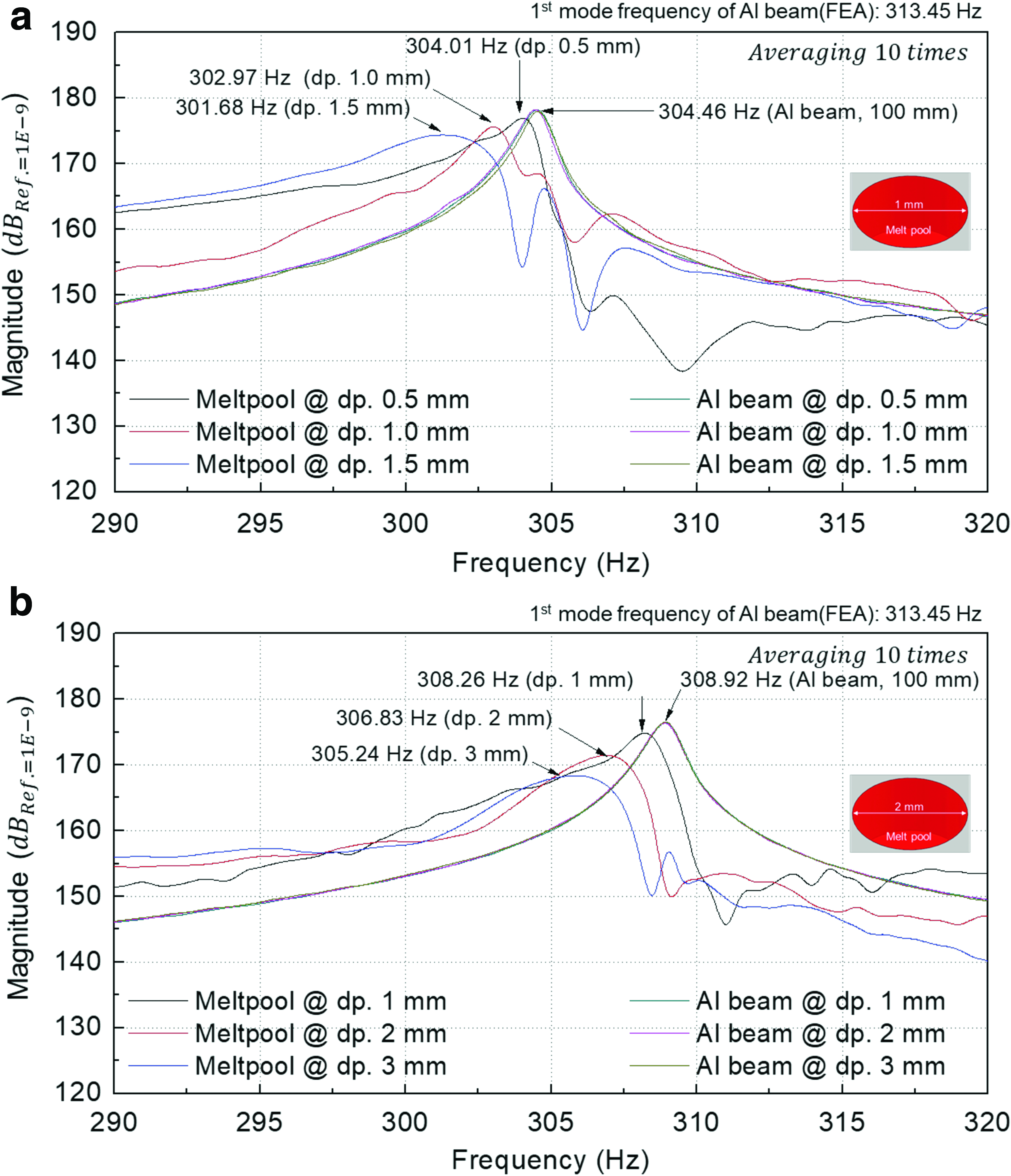
Figure 7a shows the FRF results of a melt pool of 1.0 mm diameter and the Al beam of 100 mm length. Figure 7b shows the FRF results of the melt pool of 2.0 mm diameter and the Al beam of 100 mm length. The FRF curve was acquired after 10 times averaging. The curve of \documentclass{aastex}\usepackage{amsbsy}\usepackage{amsfonts}\usepackage{amssymb}\usepackage{bm}\usepackage{mathrsfs}\usepackage{pifont}\usepackage{stmaryrd}\usepackage{textcomp}\usepackage{portland, xspace}\usepackage{amsmath, amsxtra}\usepackage{upgreek}\pagestyle{empty}\DeclareMathSizes{10}{9}{7}{6}\begin{document}
$$H{ \left( f \right) _{melt \;pool}}$$
\end{document} was shifted to the left side and the shape of \documentclass{aastex}\usepackage{amsbsy}\usepackage{amsfonts}\usepackage{amssymb}\usepackage{bm}\usepackage{mathrsfs}\usepackage{pifont}\usepackage{stmaryrd}\usepackage{textcomp}\usepackage{portland, xspace}\usepackage{amsmath, amsxtra}\usepackage{upgreek}\pagestyle{empty}\DeclareMathSizes{10}{9}{7}{6}\begin{document}
$$H{ \left( f \right) _{melt \;pool}}$$
\end{document} curve was smoother regardless of the melt pool diameter, when the melt pool depth increases from 0.5 to 1.5 D. It means that the melt pool plays a role in the damping.
FRF results according to the melt pool depth: (a) melt pool diameter is 1 mm; (b) melt pool diameter is 2 mm. FEA, finite element analysis; FRF, frequency response function. Color images are available online.
The coherence was checked to evaluate the FRF measurement test. The coherence is the function versus frequency that indicates how much of the output is due to the input in the FRF. The coherence is the index of the consistency of the FRF from the measurement when the same test is repeated. The range of the coherence function is 0 to 1. The meaning of coherence value with “1” indicates that the FRF result has highest repeatability, and the coherence value with “0” indicates that the FRF result has lowest repeatability. Figure 8 shows the coherence function graph of the measured FRF results. In the case of \documentclass{aastex}\usepackage{amsbsy}\usepackage{amsfonts}\usepackage{amssymb}\usepackage{bm}\usepackage{mathrsfs}\usepackage{pifont}\usepackage{stmaryrd}\usepackage{textcomp}\usepackage{portland, xspace}\usepackage{amsmath, amsxtra}\usepackage{upgreek}\pagestyle{empty}\DeclareMathSizes{10}{9}{7}{6}\begin{document}
$$H{ \left( f \right) _{Al \;beam}}$$
\end{document}, the coherence value is around 0.95, and the coherence value of \documentclass{aastex}\usepackage{amsbsy}\usepackage{amsfonts}\usepackage{amssymb}\usepackage{bm}\usepackage{mathrsfs}\usepackage{pifont}\usepackage{stmaryrd}\usepackage{textcomp}\usepackage{portland, xspace}\usepackage{amsmath, amsxtra}\usepackage{upgreek}\pagestyle{empty}\DeclareMathSizes{10}{9}{7}{6}\begin{document}
$$H{ \left( f \right) _{melt \;pool}}$$
\end{document} is higher than 0.6. Actually, a coherence value is typically over 0.95 for metal plates, but we measured the velocity signal on the surface of a melt pool, a kind of liquid state, so the coherence value is quite low. Through several tests, we decided that the coherence of 0.6 is also reasonable.
Representative coherence function graph of the FRF results: (a) Al beam length is 100 mm; (b) Al beam length is 50 mm. Color images are available online.
In the case of a melt pool diameter of 1 mm, the measured mean natural frequency of \documentclass{aastex}\usepackage{amsbsy}\usepackage{amsfonts}\usepackage{amssymb}\usepackage{bm}\usepackage{mathrsfs}\usepackage{pifont}\usepackage{stmaryrd}\usepackage{textcomp}\usepackage{portland, xspace}\usepackage{amsmath, amsxtra}\usepackage{upgreek}\pagestyle{empty}\DeclareMathSizes{10}{9}{7}{6}\begin{document}
$$H{ \left( f \right) _{Al \;beam \_100 \;mm}}$$
\end{document} is 304.68 Hz regardless of the melt pool depth. But the natural frequency of \documentclass{aastex}\usepackage{amsbsy}\usepackage{amsfonts}\usepackage{amssymb}\usepackage{bm}\usepackage{mathrsfs}\usepackage{pifont}\usepackage{stmaryrd}\usepackage{textcomp}\usepackage{portland, xspace}\usepackage{amsmath, amsxtra}\usepackage{upgreek}\pagestyle{empty}\DeclareMathSizes{10}{9}{7}{6}\begin{document}
$$H{ \left( f \right) _{Melt \;pool}}$$
\end{document} decreases from 304.01 to 301.68 Hz, when the melt pool depth increases from 0.5 to 1.5 mm as shown in Figure 9a. In the case of a melt pool diameter of 2 mm, the mean natural frequency of \documentclass{aastex}\usepackage{amsbsy}\usepackage{amsfonts}\usepackage{amssymb}\usepackage{bm}\usepackage{mathrsfs}\usepackage{pifont}\usepackage{stmaryrd}\usepackage{textcomp}\usepackage{portland, xspace}\usepackage{amsmath, amsxtra}\usepackage{upgreek}\pagestyle{empty}\DeclareMathSizes{10}{9}{7}{6}\begin{document}
$$H{ \left( f \right) _{Al \;beam \_100 \;mm}}$$
\end{document} is 308.92 Hz regardless of the melt pool depth. But the natural frequency of \documentclass{aastex}\usepackage{amsbsy}\usepackage{amsfonts}\usepackage{amssymb}\usepackage{bm}\usepackage{mathrsfs}\usepackage{pifont}\usepackage{stmaryrd}\usepackage{textcomp}\usepackage{portland, xspace}\usepackage{amsmath, amsxtra}\usepackage{upgreek}\pagestyle{empty}\DeclareMathSizes{10}{9}{7}{6}\begin{document}
$$H{ \left( f \right) _{Melt \;pool}}$$
\end{document} decreases from 308.26 to 305.24 Hz as the melt pool depth increases from 1 to 3 mm as shown in Figure 9b and numerical value was summarized in Table 4.
Resonance frequency results according to the melt pool diameter: (a) melt pool diameter is 1 mm; (b) melt pool diameter is 2 mm. FEM, finite element method.
Frequency Response Function Result and Modal Parameter of the Melt Pool and Al Beam
Diameter (mm)
Height (mm)
Output/input
Depth (mm)
Frequency (Hz)
Damping ratio (ζ)
1.0
50
Beam/impact
0.5
961.91
9.81E-03
1.0
960.33
9.97E-03
1.5
961.56
9.95E-03
Melt pool/impact
0.5
953.51
1.51E-02
1.0
943.35
2.48E-02
1.5
909.28
4.03E-02
100
Beam/impact
0.5
304.43
1.68E-03
1.0
304.44
1.61E-03
1.5
304.51
1.69E-03
Melt pool/impact
0.5
303.99
9.54E-04
1.0
302.87
2.99E-03
1.5
301.32
6.02E-03
2.0
50
Beam/impact
1.0
962.45
1.17E-02
2.0
963.52
1.20E-02
3.0
962.84
1.21E-02
Melt pool/impact
1.0
940.52
1.05E-02
2.0
918.68
2.16E-02
3.0
891.87
3.39E-02
100
Beam/impact
1.0
308.92
1.65E-03
2.0
308.94
1.67E-03
3.0
308.89
1.65E-03
Melt pool/impact
1.0
308.26
2.12E-03
2.0
306.83
4.76E-03
3.0
305.88
7.08E-03
The damping ratio was calculated using Eq. (3). The results were illustrated in Figure 10 and summarized in Table 3. The damping ratio of \documentclass{aastex}\usepackage{amsbsy}\usepackage{amsfonts}\usepackage{amssymb}\usepackage{bm}\usepackage{mathrsfs}\usepackage{pifont}\usepackage{stmaryrd}\usepackage{textcomp}\usepackage{portland, xspace}\usepackage{amsmath, amsxtra}\usepackage{upgreek}\pagestyle{empty}\DeclareMathSizes{10}{9}{7}{6}\begin{document}
$$H{ \left( f \right) _{Al \;beam \_100mm}}$$
\end{document} keeps it around 1.61E-03 regardless of the melt pool depth and diameter. By contrast, in the case of the melt pool diameter of 1 mm, the damping ratio of \documentclass{aastex}\usepackage{amsbsy}\usepackage{amsfonts}\usepackage{amssymb}\usepackage{bm}\usepackage{mathrsfs}\usepackage{pifont}\usepackage{stmaryrd}\usepackage{textcomp}\usepackage{portland, xspace}\usepackage{amsmath, amsxtra}\usepackage{upgreek}\pagestyle{empty}\DeclareMathSizes{10}{9}{7}{6}\begin{document}
$$H{ \left( f \right) _{Melt \;pool \_ \;1 \;mm}}$$
\end{document} increases from 0.954E-03 to 6.02E-03, when the melt pool depth increases from 0.5 to 1.5 mm. In the case of the melt pool diameter of 2 mm, the damping ratio of \documentclass{aastex}\usepackage{amsbsy}\usepackage{amsfonts}\usepackage{amssymb}\usepackage{bm}\usepackage{mathrsfs}\usepackage{pifont}\usepackage{stmaryrd}\usepackage{textcomp}\usepackage{portland, xspace}\usepackage{amsmath, amsxtra}\usepackage{upgreek}\pagestyle{empty}\DeclareMathSizes{10}{9}{7}{6}\begin{document}
$$H{ \left( f \right) _{Melt \;pool \_ \;2 \;mm}}$$
\end{document} increases from 2.12E-03 to 7.08E-03, when the melt pool depth increases from 1 to 3 mm. Table 5 shows the damping ratio according to the melt pool depth and diameter. The natural frequency and damping ratio are inversely proportional to each other as expressed in Eq. (4). This relationship provides the possibility to estimate the melt pool depth and diameter during the DED process.
Damping ratio (ζ) according to the melt pool diameter: (a) melt pool diameter is 1 mm; (b) melt pool diameter is 2 mm.
Q Factor and Damping Ratio According to the Melt Pool Depth
This section focuses on the measured natural frequency and damping ratio according to the fabricated part size. We prepared the No. 1 and No. 2 specimens as summarized in Table 2. The Al beam length was set to 50 and 100 mm while the width and thickness were fixed. The melt pool depth was controlled to 0.5 mm, 1.0 mm, and 1.5 mm, respectively, whereas the melt pool diameter was fixed at 1 mm.
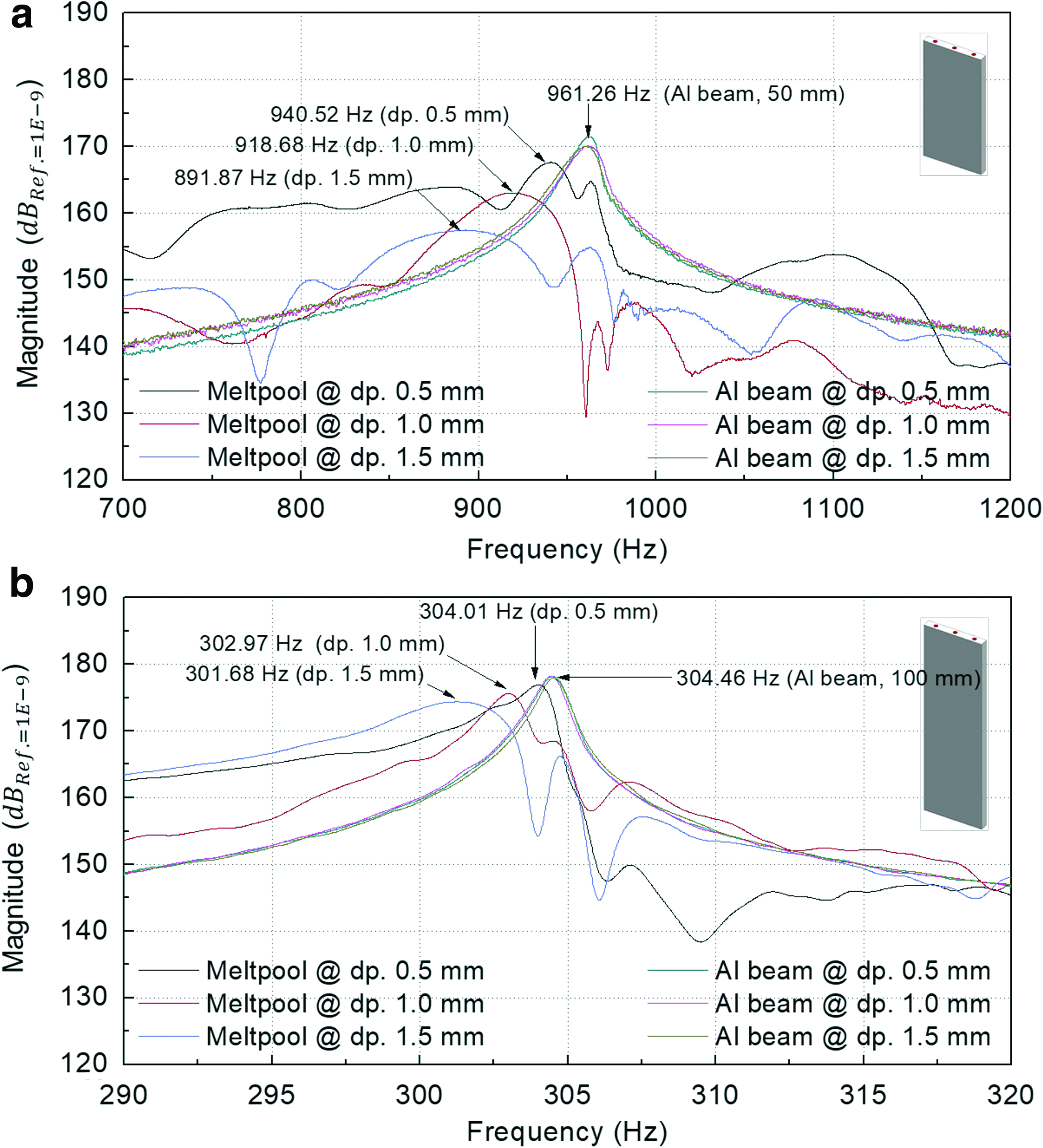
Figure 11a shows the FRF results of the Al beam of 50 mm length, and Figure 11b shows the FRF results of the Al beam of 100 mm. The FRF curve was acquired after averaging 10 times. The natural frequency of the Al beam decreased from 961.26 to 304.01 Hz. The first natural frequency peak of \documentclass{aastex}\usepackage{amsbsy}\usepackage{amsfonts}\usepackage{amssymb}\usepackage{bm}\usepackage{mathrsfs}\usepackage{pifont}\usepackage{stmaryrd}\usepackage{textcomp}\usepackage{portland, xspace}\usepackage{amsmath, amsxtra}\usepackage{upgreek}\pagestyle{empty}\DeclareMathSizes{10}{9}{7}{6}\begin{document}
$$H{ \left( f \right) _{melt \;pool \_1 \;mm}}$$
\end{document} was shifted to the lower frequency side regardless of the Al beam length, when the Al beam length increases from 50 to 100 mm. This means that the natural frequency of the pool depended on the host structure's natural frequency. The curve of \documentclass{aastex}\usepackage{amsbsy}\usepackage{amsfonts}\usepackage{amssymb}\usepackage{bm}\usepackage{mathrsfs}\usepackage{pifont}\usepackage{stmaryrd}\usepackage{textcomp}\usepackage{portland, xspace}\usepackage{amsmath, amsxtra}\usepackage{upgreek}\pagestyle{empty}\DeclareMathSizes{10}{9}{7}{6}\begin{document}
$$H{ \left( f \right) _{melt \;pool}}$$
\end{document} was shifted to left side and the peak shape of \documentclass{aastex}\usepackage{amsbsy}\usepackage{amsfonts}\usepackage{amssymb}\usepackage{bm}\usepackage{mathrsfs}\usepackage{pifont}\usepackage{stmaryrd}\usepackage{textcomp}\usepackage{portland, xspace}\usepackage{amsmath, amsxtra}\usepackage{upgreek}\pagestyle{empty}\DeclareMathSizes{10}{9}{7}{6}\begin{document}
$$H{ \left( f \right) _{melt \;pool \_1 \;mm}}$$
\end{document} curve was smoother regardless of the Al beam length, when the melt pool depth increases from 0.5 to 1.5 mm. It means that the melt pool size also plays a role in the damping.
FRF results according to the Al beam length: (a) Al beam length is 50 mm; (b) Al beam length is 100 mm. Color images are available online.
The coherence was also checked to evaluate the FRF measurement. In the case of \documentclass{aastex}\usepackage{amsbsy}\usepackage{amsfonts}\usepackage{amssymb}\usepackage{bm}\usepackage{mathrsfs}\usepackage{pifont}\usepackage{stmaryrd}\usepackage{textcomp}\usepackage{portland, xspace}\usepackage{amsmath, amsxtra}\usepackage{upgreek}\pagestyle{empty}\DeclareMathSizes{10}{9}{7}{6}\begin{document}
$$H{ \left( f \right) _{Al \;beam}}$$
\end{document}, the coherence value is around 0.9, and the coherence value of \documentclass{aastex}\usepackage{amsbsy}\usepackage{amsfonts}\usepackage{amssymb}\usepackage{bm}\usepackage{mathrsfs}\usepackage{pifont}\usepackage{stmaryrd}\usepackage{textcomp}\usepackage{portland, xspace}\usepackage{amsmath, amsxtra}\usepackage{upgreek}\pagestyle{empty}\DeclareMathSizes{10}{9}{7}{6}\begin{document}
$$H{ \left( f \right) _{melt \;pool}}$$
\end{document} is higher than 0.7.
In the case of the Al beam length of 50 mm, the mean natural frequency of \documentclass{aastex}\usepackage{amsbsy}\usepackage{amsfonts}\usepackage{amssymb}\usepackage{bm}\usepackage{mathrsfs}\usepackage{pifont}\usepackage{stmaryrd}\usepackage{textcomp}\usepackage{portland, xspace}\usepackage{amsmath, amsxtra}\usepackage{upgreek}\pagestyle{empty}\DeclareMathSizes{10}{9}{7}{6}\begin{document}
$$H{ \left( f \right) _{Al \;beam}}$$
\end{document} is 961.26 Hz regardless of the melt pool depth. But the natural frequency of \documentclass{aastex}\usepackage{amsbsy}\usepackage{amsfonts}\usepackage{amssymb}\usepackage{bm}\usepackage{mathrsfs}\usepackage{pifont}\usepackage{stmaryrd}\usepackage{textcomp}\usepackage{portland, xspace}\usepackage{amsmath, amsxtra}\usepackage{upgreek}\pagestyle{empty}\DeclareMathSizes{10}{9}{7}{6}\begin{document}
$$H{ \left( f \right) _{Melt \;pool \_1 \;mm}}$$
\end{document} decreases from 953.51 to 909.28 Hz, when the melt pool depth increases from 0.5 to 1.5 mm as shown in Figure 12a. In the case of the Al beam length of 100 mm, the mean natural frequency of \documentclass{aastex}\usepackage{amsbsy}\usepackage{amsfonts}\usepackage{amssymb}\usepackage{bm}\usepackage{mathrsfs}\usepackage{pifont}\usepackage{stmaryrd}\usepackage{textcomp}\usepackage{portland, xspace}\usepackage{amsmath, amsxtra}\usepackage{upgreek}\pagestyle{empty}\DeclareMathSizes{10}{9}{7}{6}\begin{document}
$$H{ \left( f \right) _{Al \;beam}}$$
\end{document} is 304.46 Hz regardless of the melt pool depth. But the natural frequency of \documentclass{aastex}\usepackage{amsbsy}\usepackage{amsfonts}\usepackage{amssymb}\usepackage{bm}\usepackage{mathrsfs}\usepackage{pifont}\usepackage{stmaryrd}\usepackage{textcomp}\usepackage{portland, xspace}\usepackage{amsmath, amsxtra}\usepackage{upgreek}\pagestyle{empty}\DeclareMathSizes{10}{9}{7}{6}\begin{document}
$$H{ \left( f \right) _{Melt \;pool \_1 \;mm}}$$
\end{document} decreases from 304.01 to 301.68 Hz, when the melt pool depth increases from 1 to 3 mm as shown in Figure 12b. Detailed information is summarized in Table 4.
Resonance frequency of the Al beam according to the length: (a) Al beam length is 50 mm; (b) Al beam length is 100 mm.
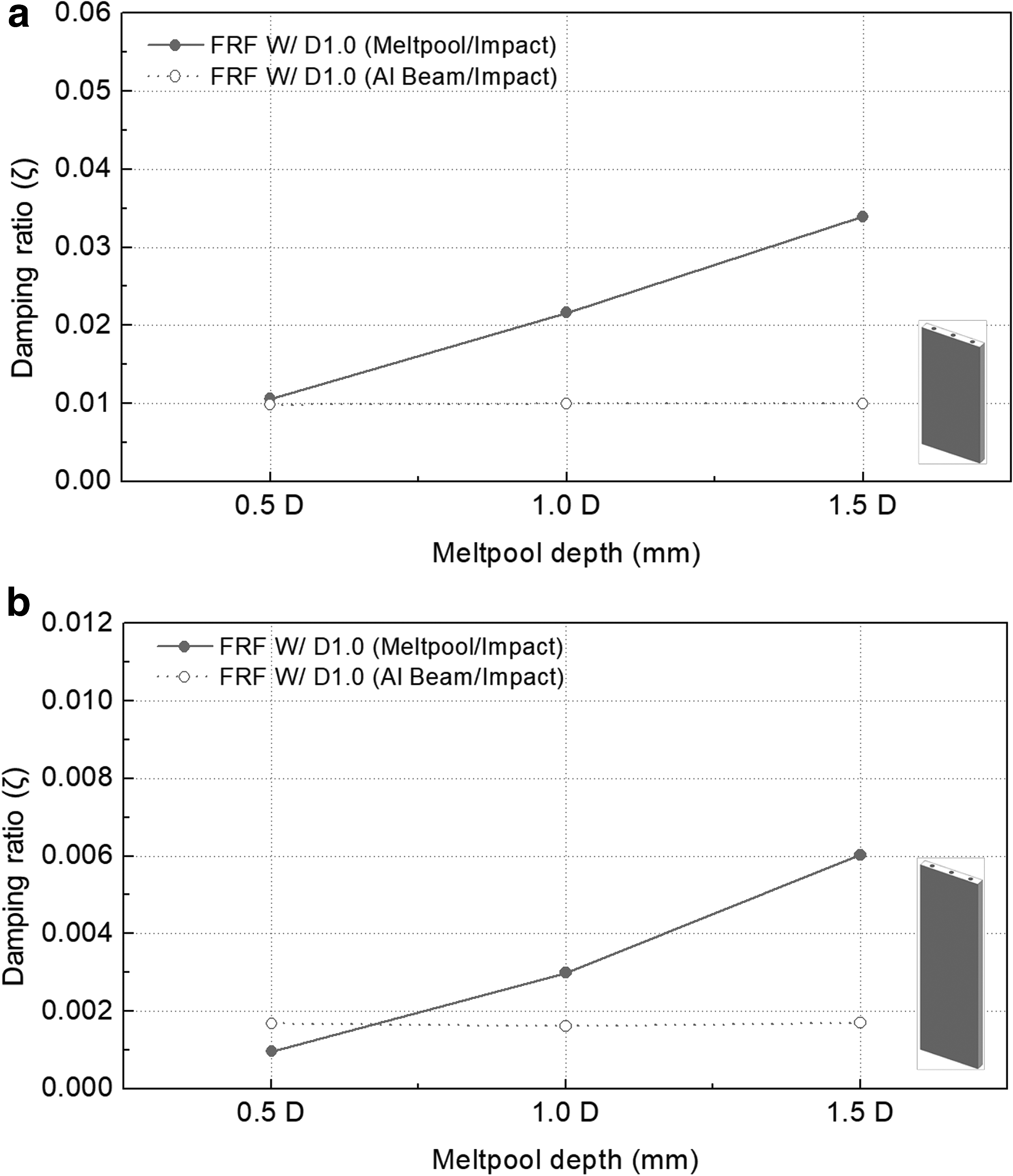
The calculated damping ratio results were illustrated in Figure 13 and summarized in Table 5. In the case of the Al beam with a length of 50 mm, the damping ratio of \documentclass{aastex}\usepackage{amsbsy}\usepackage{amsfonts}\usepackage{amssymb}\usepackage{bm}\usepackage{mathrsfs}\usepackage{pifont}\usepackage{stmaryrd}\usepackage{textcomp}\usepackage{portland, xspace}\usepackage{amsmath, amsxtra}\usepackage{upgreek}\pagestyle{empty}\DeclareMathSizes{10}{9}{7}{6}\begin{document}
$$H{ \left( f \right) _{Al \;beam \_50 \,mm}}$$
\end{document} stays around 9.81E-03 regardless of the melt pool depth and diameter. By contrast, the damping ratio of \documentclass{aastex}\usepackage{amsbsy}\usepackage{amsfonts}\usepackage{amssymb}\usepackage{bm}\usepackage{mathrsfs}\usepackage{pifont}\usepackage{stmaryrd}\usepackage{textcomp}\usepackage{portland, xspace}\usepackage{amsmath, amsxtra}\usepackage{upgreek}\pagestyle{empty}\DeclareMathSizes{10}{9}{7}{6}\begin{document}
$$H{ \left( f \right) _{Melt \;pool \_ \;1 \;mm}}$$
\end{document} increases from 1.51E-02 to 4.03E-02, when the melt pool depth increases from 0.5 to 1.5 mm as shown in Figure 13a. In the case of the Al beam length of 100 mm, the damping ratio of \documentclass{aastex}\usepackage{amsbsy}\usepackage{amsfonts}\usepackage{amssymb}\usepackage{bm}\usepackage{mathrsfs}\usepackage{pifont}\usepackage{stmaryrd}\usepackage{textcomp}\usepackage{portland, xspace}\usepackage{amsmath, amsxtra}\usepackage{upgreek}\pagestyle{empty}\DeclareMathSizes{10}{9}{7}{6}\begin{document}
$$H{ \left( f \right) _{Al \;beam \_100 \,mm}}$$
\end{document} keeps around 1.61E-03 regardless of the melt pool depth and diameter. On the contrary, the damping ratio of \documentclass{aastex}\usepackage{amsbsy}\usepackage{amsfonts}\usepackage{amssymb}\usepackage{bm}\usepackage{mathrsfs}\usepackage{pifont}\usepackage{stmaryrd}\usepackage{textcomp}\usepackage{portland, xspace}\usepackage{amsmath, amsxtra}\usepackage{upgreek}\pagestyle{empty}\DeclareMathSizes{10}{9}{7}{6}\begin{document}
$$H{ \left( f \right) _{Melt \;pool \_ \;1 \;mm}}$$
\end{document} increases from 0.954E-03 to 6.02E-03, when the melt pool depth increases from 0.5 to 1.5 mm as shown in Figure 13b.
Damping ratio (ζ) according to the Al beam length: (a) Al beam length is 50 mm; (b) Al beam length is 100 mm.
Through the experimental results, we confirmed that the melt pool depth can be estimated using damped natural frequency and damping ratio regardless of the host structure size. The natural frequency of the host structure can be obtained using analytical methods such as finite element analysis, and the data can be used as a reference to check the melt pool states during the DED process.
Discussion
Measurement point of the melt pool effect
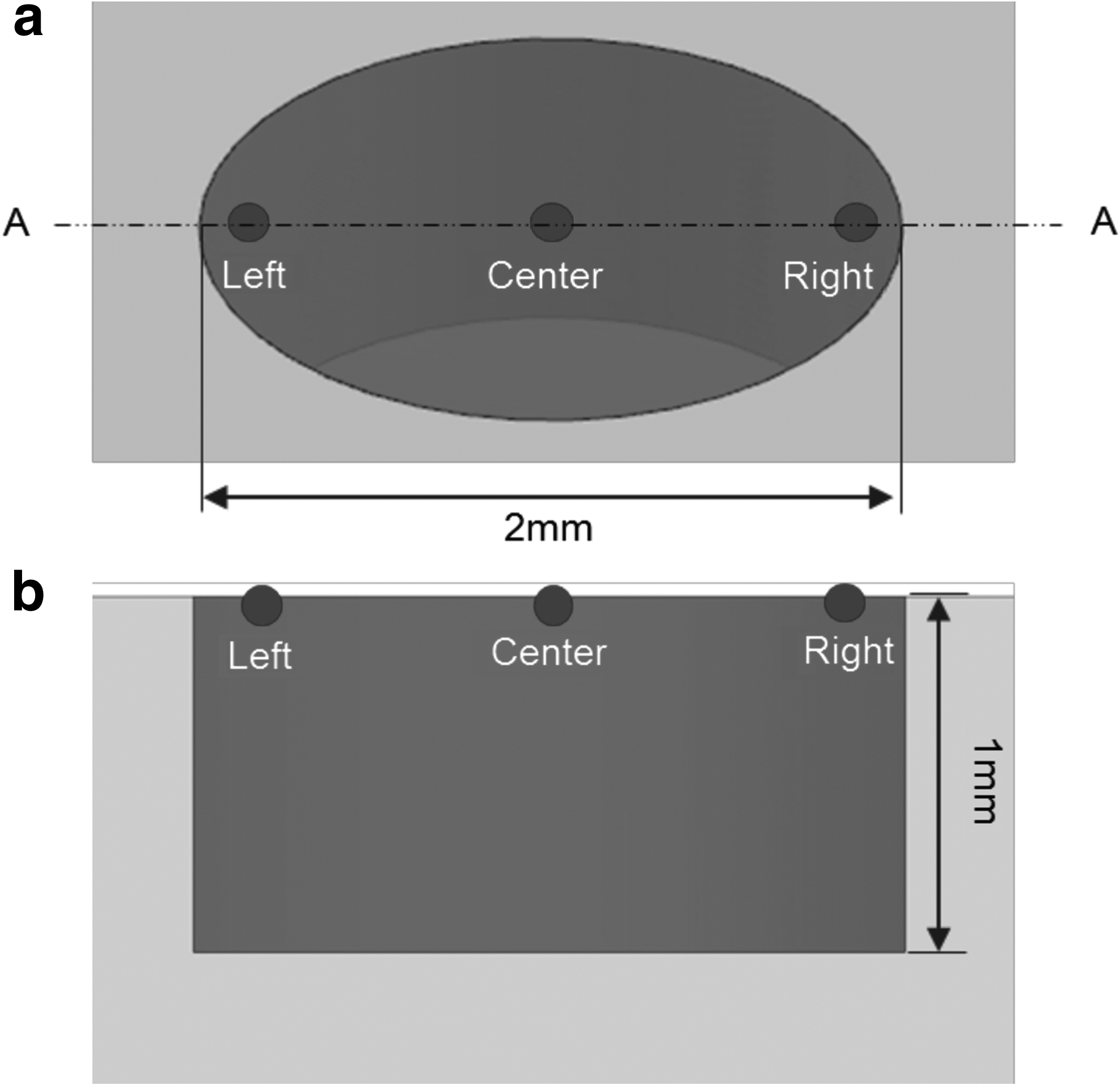
This section focuses the measurement point effect on the first natural frequency and damping ratio. To perform this test, the melt pool depth was fixed at 2 mm, the depth was fixed at 1 mm, and the length of the Al beam was fixed at 105 mm, whereas the measurement points were set with three points, such as left side, center, and right side of the melt pool, as illustrated in Figure 14.
Measurement point of the melt pool: (a) The top view; (b) The section view of A-A.
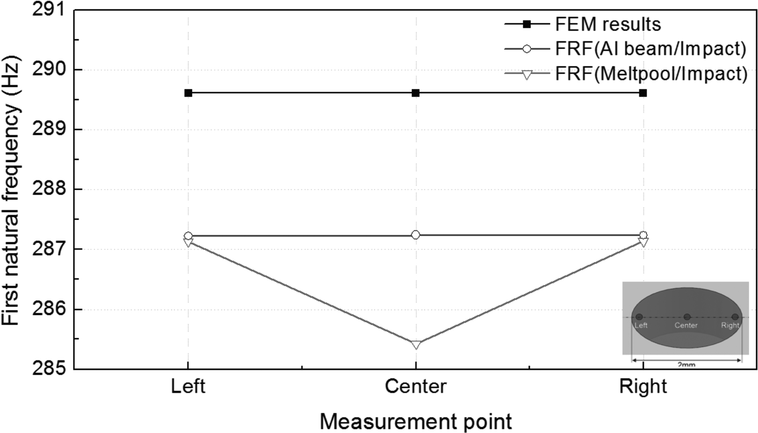
The mean natural frequency of \documentclass{aastex}\usepackage{amsbsy}\usepackage{amsfonts}\usepackage{amssymb}\usepackage{bm}\usepackage{mathrsfs}\usepackage{pifont}\usepackage{stmaryrd}\usepackage{textcomp}\usepackage{portland, xspace}\usepackage{amsmath, amsxtra}\usepackage{upgreek}\pagestyle{empty}\DeclareMathSizes{10}{9}{7}{6}\begin{document}
$$H{ \left( f \right) _{Al \;beam}}$$
\end{document} is 287.23 Hz regardless of the melt pool measurement point. The first natural frequency of \documentclass{aastex}\usepackage{amsbsy}\usepackage{amsfonts}\usepackage{amssymb}\usepackage{bm}\usepackage{mathrsfs}\usepackage{pifont}\usepackage{stmaryrd}\usepackage{textcomp}\usepackage{portland, xspace}\usepackage{amsmath, amsxtra}\usepackage{upgreek}\pagestyle{empty}\DeclareMathSizes{10}{9}{7}{6}\begin{document}
$$H{ \left( f \right) _{left \;side \;of \;melt \;pool}}$$
\end{document} is 287.13 Hz. The first natural frequency of \documentclass{aastex}\usepackage{amsbsy}\usepackage{amsfonts}\usepackage{amssymb}\usepackage{bm}\usepackage{mathrsfs}\usepackage{pifont}\usepackage{stmaryrd}\usepackage{textcomp}\usepackage{portland, xspace}\usepackage{amsmath, amsxtra}\usepackage{upgreek}\pagestyle{empty}\DeclareMathSizes{10}{9}{7}{6}\begin{document}
$$H{ \left( f \right) _{center \;of \;melt \;pool}}$$
\end{document} decreases to 285.43 Hz. On the other hand, the first natural frequency of \documentclass{aastex}\usepackage{amsbsy}\usepackage{amsfonts}\usepackage{amssymb}\usepackage{bm}\usepackage{mathrsfs}\usepackage{pifont}\usepackage{stmaryrd}\usepackage{textcomp}\usepackage{portland, xspace}\usepackage{amsmath, amsxtra}\usepackage{upgreek}\pagestyle{empty}\DeclareMathSizes{10}{9}{7}{6}\begin{document}
$$H{ \left( f \right) _{right \;side \;of \;melt \;pool}}$$
\end{document} increases to 287.14 Hz as illustrated in Figure 15, and summarized in Table 6.
First natural frequency according to the measurement point.
Relationship Between Resonance Frequency and Damping Ratio According to the Measurement Point
Output/input
Measurement point
Frequency (Hz)
Damping ratio (ζ)
Beam/impact
left
287.22
2.263E-03
center
287.24
2.454E-03
right
287.23
2.141E-03
Melt pool/impact
left
287.13
2.403E-03
center
285.43
3.749E-03
right
287.1
2.299E-03
The damping ratio of \documentclass{aastex}\usepackage{amsbsy}\usepackage{amsfonts}\usepackage{amssymb}\usepackage{bm}\usepackage{mathrsfs}\usepackage{pifont}\usepackage{stmaryrd}\usepackage{textcomp}\usepackage{portland, xspace}\usepackage{amsmath, amsxtra}\usepackage{upgreek}\pagestyle{empty}\DeclareMathSizes{10}{9}{7}{6}\begin{document}
$$H{ \left( f \right) _{Al \;beam}}$$
\end{document} keeps around 2.141E-03 to 2.403E-03 regardless of the melt pool measurement points. The damping ratio of \documentclass{aastex}\usepackage{amsbsy}\usepackage{amsfonts}\usepackage{amssymb}\usepackage{bm}\usepackage{mathrsfs}\usepackage{pifont}\usepackage{stmaryrd}\usepackage{textcomp}\usepackage{portland, xspace}\usepackage{amsmath, amsxtra}\usepackage{upgreek}\pagestyle{empty}\DeclareMathSizes{10}{9}{7}{6}\begin{document}
$$H{ \left( f \right) _{left \;side \;of \;melt \;pool}}$$
\end{document} is 2.403E-03, the damping ratio of \documentclass{aastex}\usepackage{amsbsy}\usepackage{amsfonts}\usepackage{amssymb}\usepackage{bm}\usepackage{mathrsfs}\usepackage{pifont}\usepackage{stmaryrd}\usepackage{textcomp}\usepackage{portland, xspace}\usepackage{amsmath, amsxtra}\usepackage{upgreek}\pagestyle{empty}\DeclareMathSizes{10}{9}{7}{6}\begin{document}
$$H{ \left( f \right) _{center \;of \;melt \;pool}}$$
\end{document} is 3.749E-03, and the damping ratio of \documentclass{aastex}\usepackage{amsbsy}\usepackage{amsfonts}\usepackage{amssymb}\usepackage{bm}\usepackage{mathrsfs}\usepackage{pifont}\usepackage{stmaryrd}\usepackage{textcomp}\usepackage{portland, xspace}\usepackage{amsmath, amsxtra}\usepackage{upgreek}\pagestyle{empty}\DeclareMathSizes{10}{9}{7}{6}\begin{document}
$$H{ \left( f \right) _{right \;side \;of \;melt \;pool}}$$
\end{document} is 2.299E-03 as illustrated in Figure 16 and summarized in Table 5. These results indicate that the natural frequency decreases, but the damping ratio increases, at velocity measurement points far from the boundary of the melt pool. According to this result, the measurement point of the melt pool is also a major factor to estimate the melt pool depth. If we measure the velocity at the same point, this deviation can be ignored, so that we can propose to measure the velocity at the center of the melt pool, which shows the largest damping effect and largest frequency deviation compared with those of host structure.
Damping ratio \documentclass{aastex}\usepackage{amsbsy}\usepackage{amsfonts}\usepackage{amssymb}\usepackage{bm}\usepackage{mathrsfs}\usepackage{pifont}\usepackage{stmaryrd}\usepackage{textcomp}\usepackage{portland, xspace}\usepackage{amsmath, amsxtra}\usepackage{upgreek}\pagestyle{empty}\DeclareMathSizes{10}{9}{7}{6}\begin{document}
$$( {\rm{{\upzeta} }} )$$
\end{document} according to the measurement point.
Conclusion
In this study, the in-situ melt pool size monitoring method is proven to be applicable to the commercial AM process. The test set-up consists of two LDV systems, an impact hammer, and data acquisition device together with data capturing and FRF software. The data from each sensor was processed to compute the natural frequency and damping ratio, which is influenced by the melt pool depth, diameter, and length of Al beam. We found that the relationship between the first natural frequency and damping ratio is as follows:
(1) In the case of the Al beam with 50 mm length and melt pool diameter with 1 mm, the natural frequency of \documentclass{aastex}\usepackage{amsbsy}\usepackage{amsfonts}\usepackage{amssymb}\usepackage{bm}\usepackage{mathrsfs}\usepackage{pifont}\usepackage{stmaryrd}\usepackage{textcomp}\usepackage{portland, xspace}\usepackage{amsmath, amsxtra}\usepackage{upgreek}\pagestyle{empty}\DeclareMathSizes{10}{9}{7}{6}\begin{document}
$$H{ \left( f \right) _{Melt \;pool \_1 \,mm}}$$
\end{document} decreases from 953.51 to 909.28 Hz, whereas the damping ratio increases from 1.51E-02 to 4.03E-02 linearly, when the melt pool depth increases from 0.5 to 1.5 mm linearly.
(2) In the case of the Al beam with 100 mm length and melt pool diameter with 1 mm, the natural frequency of \documentclass{aastex}\usepackage{amsbsy}\usepackage{amsfonts}\usepackage{amssymb}\usepackage{bm}\usepackage{mathrsfs}\usepackage{pifont}\usepackage{stmaryrd}\usepackage{textcomp}\usepackage{portland, xspace}\usepackage{amsmath, amsxtra}\usepackage{upgreek}\pagestyle{empty}\DeclareMathSizes{10}{9}{7}{6}\begin{document}
$$H{ \left( f \right) _{Melt \;pool \_1 \,mm}}$$
\end{document} decreases from 303.99 to 301.32 Hz, whereas the damping ratio increases from 0.95E-03 to 6.02E-03 linearly, when the melt pool depth increases from 0.5 to 1.5 mm linearly.
(3) In the case of the Al beam with 50 mm length and melt pool diameter with 2 mm, the natural frequency of \documentclass{aastex}\usepackage{amsbsy}\usepackage{amsfonts}\usepackage{amssymb}\usepackage{bm}\usepackage{mathrsfs}\usepackage{pifont}\usepackage{stmaryrd}\usepackage{textcomp}\usepackage{portland, xspace}\usepackage{amsmath, amsxtra}\usepackage{upgreek}\pagestyle{empty}\DeclareMathSizes{10}{9}{7}{6}\begin{document}
$$H{ \left( f \right) _{Melt \;pool \_2mm}}$$
\end{document} decreases from 940.52 to 891.87 Hz, whereas the damping ratio increases from 1.05E-02 to 3.39E-02 linearly, when the melt pool depth increases from 1 to 3 mm linearly.
(4) In the case of the Al beam with 100 mm length and melt pool diameter with 2 mm, the natural frequency of \documentclass{aastex}\usepackage{amsbsy}\usepackage{amsfonts}\usepackage{amssymb}\usepackage{bm}\usepackage{mathrsfs}\usepackage{pifont}\usepackage{stmaryrd}\usepackage{textcomp}\usepackage{portland, xspace}\usepackage{amsmath, amsxtra}\usepackage{upgreek}\pagestyle{empty}\DeclareMathSizes{10}{9}{7}{6}\begin{document}
$$H{ \left( f \right) _{Melt \;pool \_2 \,mm}}$$
\end{document} decreases from 308.26 to 305.88 Hz, whereas the damping ratio increases from 2.12E-03 to 7.08E-03 linearly, when the melt pool depth increases from 1 to 3 mm linearly.
(5) The natural frequency decreases but damping ratio increases, when the velocity measurement point moves from the boundary of the melt pool to the center of the melt pool.
The experimental set-up in this study enables the DED machine to log the estimated melt pool depth, as well as the first natural frequency of the host structure in real-time. These data can also be used for feedback control to ensure manufacturing quality. For this, further studies could include applying the melt pool size estimation algorithm to the real additive manufacturing system, which compares the measured modal components with reference data obtained from finite element analysis as show in Figure 2b.
Footnotes
Acknowledgments
This research was supported by the Leading Human Resource Training Program of Regional Neo Industry (2016H1D5A1910063) through the National Research Foundation of Korea funded by the Ministry of Science, ICT, and Future Planning, and a grant (20170914-C3-006) from Jeonbuk Research & Development Program funded by Jeonbuk Province.
Author Disclosure Statement
No competing financial interests exist.
References
1.
WallerJM, ParkerBH, HodgesKL, et al.Nondestructive Evaluation of Additive Manufacturing Report. Hampton, VA: National Aeronautics and Space Administration, 2014.
2.
NowotnyS, ScharekS, BeyerE, et al.Laser beam build-up welding: precision in repair, surface cladding, and direct 3D metal deposition. J Therm Spray Techn, 2007; 16:344–348.
3.
KruthJ-P, MercelisP, Van VaerenberghJ, et al.Binding mechanisms in selective laser sintering and selective laser melting. Rapid Prototyp J, 2005; 11:26–36.
4.
MelchelsFP, DomingosMA, KleinTJ, et al.Additive manufacturing of tissues and organs. Prog Polym Sci, 2012; 37:1079–1104.
5.
ASTM Committee F42 on Additive Manufacturing Technologies, and ASTM Committee F42 on Additive Manufacturing Technologies. Subcommittee F42.91 on Terminology. Standard terminology for additive manufacturing technologies. West Conshohocken, PA: ASTM International. DOI: 101520/F2792-12. 2012. See www.astm.org
6.
HankeR, FuchsT, UhlmannN. X-ray based methods for non-destructive testing and material characterization. Nucl Instrum Methods Phys Res A, 2008; 591:14–18.
7.
SekharV, NeoS, YuLH, et al.Non-destructive testing of a high dense small dimension through silicon via (TSV) array structures by using 3D X-ray computed tomography method (CT scan). 201012th Electronics Packaging Technology Conference (EPTC). IEEE, Singapore, 2010; pp. 462–466.
8.
BartkowiakK.Direct laser deposition process within spectrographic analysis in situ. Phys Proc, 2010; 5:623–629.
9.
SongL, MazumderJ. Real time Cr measurement using optical emission spectroscopy during direct metal deposition process. IEEE Sens J, 2012; 12:958–964.
10.
SongL, WangC, MazumderJ. Identification of phase transformation using optical emission spectroscopy for direct metal deposition process. Spie Lase: International Society for Optics and Photonics, San Francisco, CA, 2012;8239:82390G.
11.
ZenzingerG, BambergJ, LadewigA, et al.Process monitoring of additive manufacturing by using optical tomography. AIP Conf Proc, 2015:164–170.
12.
KromineA, FomitchovP, KrishnaswamyS, et al.Laser ultrasonic detection of surface breaking discontinuities: scanning laser source technique. Mater Eval, 2000; 58:173–177.
13.
EdwardsRS, DuttonB, CloughA, et al.Scanning laser source and scanning laser detection techniques for different surface crack geometries. AIP Conf Proc, 2012:251–258.
14.
CernigliaD, ScafidiM, PantanoA, et al.Laser ultrasonic technique for laser powder deposition inspection. Laser, 2013; 6:13.
15.
GuanG, HirschM, LuZH, et al.Evaluation of selective laser sintering processes by optical coherence tomography. Mater Des, 2015; 88:837–846.
16.
RangaswamyP, HoldenT, RoggeR, et al.Residual stresses in components formed by the laserengineered net shaping (LENS®) process. J Strain Anal Eng Des, 2003; 38:519–527.
17.
RichardsonMH, FormentiDL. Global curve fitting of frequency response measurements using the rational fraction polynomial method. Proceedings of the Third International Modal Analysis Conference (IMAC). 1985; pp. 390–397.
18.
ThompsonSM, BianL, ShamsaeiN, et al.An overview of direct laser deposition for additive manufacturing; Part I: Transport phenomena, modeling and diagnostics. Addit Manuf, 2015; 8:36–62.
19.
WolffS, LeeT, FaiersonE, et al.Anisotropic properties of directed energy deposition (DED)-processed Ti–6Al–4V. J Manuf Process, 2016; 24:397–405.
20.
ChengB, ChouK.Melt pool geometry simulations for powder-based electron beam additive manufacturing. 24th Annual International Solid Freeform Fabrication Symposium-An Additive Manufacturing Conference. Austin, TX: University of Texas, 2013:644–654.
21.
GockelJ, BeuthJ, TamingerK. Integrated control of solidification microstructure and melt pool dimensions in electron beam wire feed additive manufacturing of Ti-6Al-4V. Addit Manuf, 2014; 1:119–126.
22.
ThyagarajanS, SchulzM, PaiP, et al.Detecting structural damage using frequency response functions. J Sound Vib, 1998; 210:162–170.