Regenerative Topology Optimization of Fine Lattice Structures

Abstract

We present a generative approach for creating three-dimensional lattice structures optimized for mass and deflection composed of thousands of one-dimensional strut primitives. Our approach draws inspiration from topology optimization principles. The proposed method iteratively determines unnecessary lattice struts through stress analysis, erodes those struts, and then randomly generates new struts across the entire structure. The objects resulting from this distributed optimization technique demonstrate high strength-to-weight ratios that are at par with state-of-the-art topology optimization approaches, but are qualitatively very different. We use a dynamics simulator that allows optimization of structures subject to dynamic load cases, such as vibrating structures and robotic components. Because optimization is performed simultaneously with simulation, the process scales efficiently on massively parallel graphics processing units. The intricate nature of the output lattices contributes to a new class of objects intended specifically for additive manufacturing. Our work contributes a highly parallel simulation method and simultaneous algorithm for analyzing and optimizing lattices with thousands of struts. In this study, we validate multiple versions of our algorithm across sample load cases, to show its potential for creating high-resolution objects with implicit optimized microstructural patterns.

Introduction

One of the primary goals of structural design automation is to achieve the strongest structure with the least possible material. As additive manufacturing (AM) has flourished as a fabrication technique, latticed structures have emerged as an area of exploration in generative design for their unique mechanical properties and lightweight nature. Lattice structures—structures created by connected struts and/or tiled geometric primitives—are often easier to fabricate through AM than more traditional methods. However, lattices are difficult to generate given a mechanical goal because of their often fine and intricate geometry relative to the overall size of the structure. For these reasons, we have developed an optimization technique for lattices under mechanical load cases, one that operates directly on lattices and lattice primitives.

Topology optimization and shape optimization techniques have been used across engineering disciplines since the 1980's¹ to create structures optimized to their specific environments and use cases. However, it is particularly AM's ability to manufacture objects, which are customized and porous, along with the development of high-performance computational hardware, which lends topology and shape optimization to designing structures with these properties.² The reader is directed to Doubrovski et al.² and Liu et al.³ for survey articles that elaborate on this connection in recent work.

Over the last three decades, research in topology optimization has been massively transformative in creating computer-generated structures that satisfy diverse design constraints. Topology optimization methods typically work by defining a minimization or maximization problem (often minimizing compliance under a volume constraint), analyzing a continuous design space using the Finite Element Method, and adjusting the amount of material used in the resulting structure based on this analysis.⁴ Finite voxel elements are often assigned a density value based on their necessity in the resulting design. Techniques such as these have seen success in many applications in engineering and design. However, topology optimization techniques have struggled with creating fine features as discussed above.⁵

Topology optimization is typically performed at some finite voxel resolution, and thus it would be necessary to use an extremely refined voxel grid to create smooth and thin features. This process of using a voxel primitive requires immense computational power and time to create detailed forms, especially for large-scale structures.⁶

In this study, we propose the use of a linear rod primitive, restricting the input and output space to latticed structures, along with a relaxation-based mass–spring simulation engine, which can innately handle large-scale structures through parallelism. As the scale of optimized structures has been increasing,⁷ creating microstructure has been investigated as an open problem in the field.

Recent advances in topology optimization have focused on achieving detailed microstructural structures in large structures, which given the challenges posed by an finite element analysis (FEA) method, has been achieved with ultra-high-performance supercomputers,^6,7 sparse grid techniques,⁵ and high-resolution smoothing.⁸ These works have been highly successful at producing functional, detailed, and esthetically pleasing designs using gradient-based topology optimization techniques. However, methods based on FEA are dependent upon the coarseness of the mesh, and for the average user, this leads to high computational costs associated with achieving a detailed high-resolution design.

Our method uses a non-FEA simulation approach to operate on base primitives as a limiting unit,⁹ rather than voxels. This allows us to achieve fine structural properties with low computational cost. Because our technique is based on a “Ground Structure” approach,^10,11 our result of only culling this initial network of elements is limited to the initial configuration. To combat this, we also present a technique that allows regeneration of primitives in novel locations, but which is less computationally efficient than our material removal method.

Several articles have explored the use of alternative primitives in creating forms through topology optimization. Rectangular geometries have been studied as nongridded representations in two-dimensional (2D), where rectangles and rectangular solids are rotated and resized, related by connection networks that ensure a valid final design.^12,13 A similar representation was used by Norato et al., who used 2D rectangles with capping circles as primitives.¹⁴ The success of such methods demonstrates the advantages of capturing common output structural components natively through discrete primitives that resemble bar-like support structure.

Because our method uses cylindrical struts as structural primitives, our approach bears relation to the field of truss optimization. Optimal trusses were notably explored in A. G. M. Michell's work formulating the eponymous Michell trusses. Michell proved that frames (composed of struts with uniform cross-sections¹⁵) under load and mass constraint minimize compliance by aligning proportionally to the resulting strain.¹⁶ Many truss optimization solutions echo Michell trusses visually by demonstrating similar resulting structures.¹⁷ Notably in recent work, Arora et al. demonstrated a method that parametrically generates trusses that follow Michell's model, allowing for the creation of optimized three-dimensional (3D) lattices of uniform density.¹⁸

The resulting lattices are volume constrained to an input geometry, with strut width and cross-lattice spacing controlled by the user. Their physical success is demonstrated against the results of other truss optimization techniques. Note that while revolutionary, Michell trusses have been analyzed in several works and found to be unoptimal on the basis that they restrict the output space of structures to regular trusses.^15,19 Our method does not restrict an output lattice to a regular spacing of struts. Rather than explicitly choosing the placement of cross-struts for bracing, our use of simultaneous simulation and optimization creates both support and bracing implicitly.

The goals of truss optimization are often to create structures of fewer design elements than ours, and thus are able to use more computationally expensive methods, which are guaranteed to converge to an optimal structure. Stolpe²⁰ gives an excellent review of truss optimization techniques since the 1970s (and earlier). Our method uses a heuristic to iteratively and continuously optimize structures. This continuous optimization and simulation technique can be found in the truss optimization strategy by Gutkowski et al.²¹ Our method takes this approach to a larger scale, on the order of hundreds of thousands of initial truss elements, to capture fewer regular geometries and smaller features. We direct the reader to Figure 1 for several 3D printed results of our method. Our contributions are as follows:

FIG. 1.

Four photographs of (a) a 3D printed cantilever beam run to mid optimization (50 iterations) with strut removal and regeneration, (b) a 3D printed bracket from the GE Bracket Challenge optimized with strut removal, (c) a 3D printed bracket from the GE Bracket Challenge optimized with volume-bounded strut regeneration, and (d) a cross-section of a bouncing cube run with dynamic strut removal. 3D, three-dimensional.

An efficient simulation technique for lattices with thousands of struts.

Two iterative optimization procedures for co-optimizing the strength-to-weight ratio of these lattices.

Validation and performance comparison of our results against other optimization methods.

Methods

The discretization technique provides us with a set of interconnected one-dimensional struts. The strut connectivity graph can be represented by a $a \times b$ matrix, G, where a is the number of mass nodes and b is the number of struts.

Lattice initialization

We have two primary methods for lattice initialization: (1) cubic discretization, and (2) quasi-random discretization. Figure 2 shows these two algorithms in practice, generating lattices from a femur design space. Cubic discretization provides good directional clarity when viewing the forces. However, we chose to use a quasi-random generative lattice as our standard initialization because this randomness is inherent in our regenerative evolution steps. Therefore, randomness in the initialization was not only more convenient, but more robust during testing. Other lattice initializations are possible and might provide advantages for certain designs; for example, a hexagonal discretization might be preferred over cubic for increased stability. We discuss these lattice generation methods in more detail in Supplementary Appendix SA1.

FIG. 2.

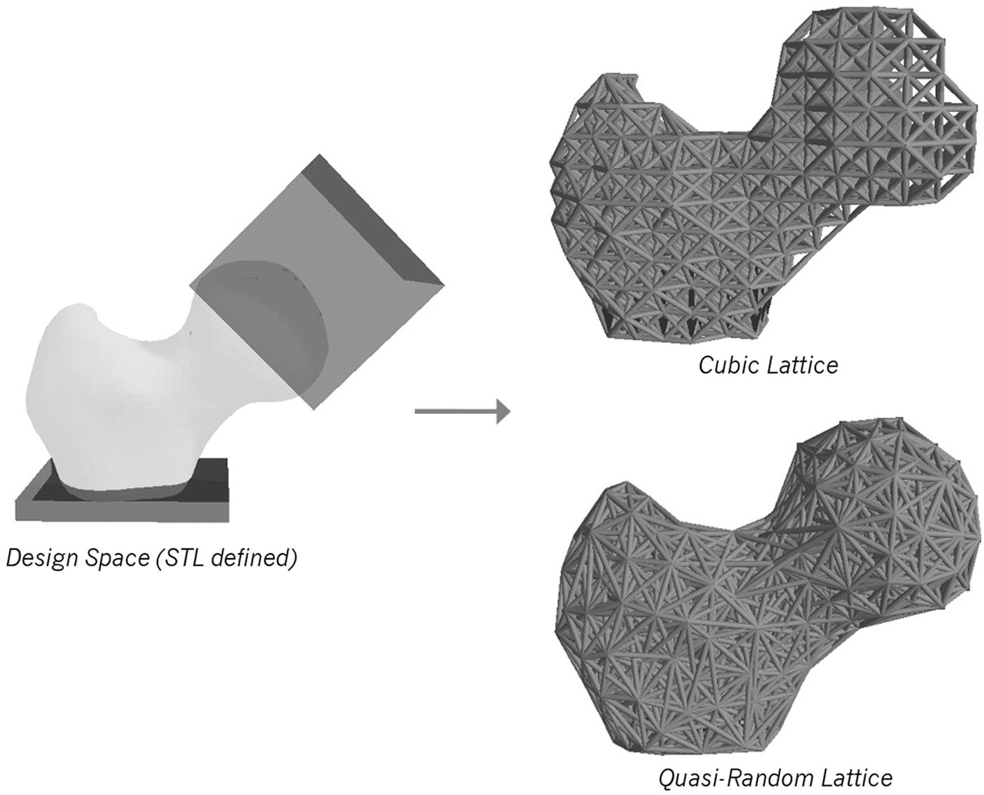
A diagram demonstrating the two methods of lattice initialization that we utilize on a femur model. The design space on the left is converted from volumetric mesh to the lattices on the right. The upper right shows a cubic lattice and the bottom right shows a quasi-random lattice.

Simulation

We take a user-defined elasticity modulus, E, and strut diameter, x, to derive our simulation variables. Note that through the mass–spring system we use, each strut could potentially have its own value for each parameter, or even functional values, allowing for the simulation of highly nonlinear materials. In this article, we will only be exploring isotropic, uniform materials and strut diameters. We derive a spring constant algebraically, k, for each strut as shown below: $F = k (∥ s ∥ - ∥ s_{0} ∥) \frac{s}{∥ s ∥} a n d δ = \frac{∥ s ∥ - ∥ s_{0} ∥}{∥ s_{0} ∥} = \frac{∥ F ∥}{A E} .$ (1) $k = \frac{A δ E}{∥ s ∥ - ∥ s_{0} ∥} = \frac{A E}{∥ s_{0} ∥} .$ (2)

We model our struts as linear and uniform, which gives us the well-known equations shown in Equation (1), namely Hooke's Law and the definitions of tensile strain. $s$ represents the vector corresponding to a strut, where $s$ is the vector from the strut's left mass position to right mass position. $∥ s_{0} ∥$ represents the original length of the strut and $∥ s ∥$ represents the current length of the strut. We define $F$ as the force vector that will be applied to the right mass (while $- F$ will be applied to the left mass) and A as cross-sectional area. $δ$ is defined as tensile strain.

While the springs only accurately model beams in their axial direction (i.e., forces are iteratively applied locally), the entire system is able to exhibit emergent behaviors at the larger scale.²² This allows our strategy to capture macrophenomena in the simulated structure as a whole, such as bending and twisting.

We use a GPU-parallelized mass–spring simulation engine⁹ to model lattices. Because calculations are done in parallel with each mass updated separately, we are able to use a small-enough time step that a semi-implicit Euler integration scheme provides an accurate and computationally inexpensive time integration. Simulations were performed on a NVIDIA Titan Xp GPU card with an Intel Core i7-8700K CPU unless stated otherwise.

Problem formulation

Given a 3D design domain $Ω$ with strut configuration B, we want to minimize total deflection, $δ_{T}$ , that is, the sum of the displacements, $δ_{0 \dots e}$ , of loaded mass nodes from an initial position.

minimize $δ_{T} = \sum_{i = 0}^{i < a} δ_{i},$ (3)

subject to $M (B) = \sum_{j = 0}^{j < b} m_{j} \leq M^{*},$ (4)

where B represents the set of individual struts (with the properties enumerated above). m_j refers to the mass of strut number j. $M^{*}$ refers to the user-provided mass threshold (as a percentage of original mass) defining the target remaining material for the optimization.

Algorithm 1. Optimization procedure
Requrie: $m o d e l_{i n}$ ▹ Input design space
$s \leftarrow I n i t i a l i z e L a t t i c e (m o d e l_{i n})$ ▹ Returns strut positions
$R e l a x (s)$
if regeneration is true then
$R e g e n e r a t e S t r u t s (s, y, v)$ ▹ Regenerates y% of struts. If v is true constrain regeneration space to $m o d e l_{i n} .$
$R e l a x (s)$
end if
while $M (B) > M^{<} s u p > * < ∕ s u p >$ do
$R e m o v e S t r u t s B y S t r e s s (s, x)$ ▹ Removes x% of struts by lowest stress
$R e l a x (s)$
end while

Structural modification technique

The addition and removal of struts proceeds in a stepwise fashion between relaxation intervals. If strut regeneration is used, optimization will take the form of: cull then relax until a user-defined target mass threshold is reached, then regenerate through stochastic search followed by relaxation. This process is repeated for set amount of wall clock time or a target number of search iterations is completed. If strut regeneration is not used, we relax and cull the structure until our target mass threshold is reached, at which point the simulation concludes.

Below we outline the specific techniques behind culling and regeneration through mutation. Culling on its own achieves dramatic weight loss and effective structures. However, the iterative interspersal between culling and regeneration searches and evaluates each strut as a part of the final lattice structure, converging to an optimal state.

Culling the lattice topology

The lattice topology is culled iteratively through the creation of a stepped removal threshold (see Smith et al.²³ for a similar example that culls truss structures in this manner.) During time integration, each strut object locally saves its maximum stress experienced, as defined by $σ_{m a x} = m a x (k | l_{0} - l |, σ_{m a x} ∕ A)$ . k represents the strut-specific spring constant, l is the current length of the strut, l₀ is the rest length of the strut, and A is the cross-sectional area of the strut (which is constant in our system, so we drop this term during calculation). After relaxation, we sort the strut $σ_{m a x}$ values, and note the minimum $β * b$ strut connections $\in B$ where $β$ is our culling threshold, $0 \leq β \leq 1$ , and b is the size of B. Once the $β * b$ struts with the smallest $σ_{m a x}$ values are noted, we mark these struts as invalid. Additionially we recursively cull struts that are poorly joined to the lattice topology. Please see Appendix B for more details about culling these edge cases.

Regenerating lattice topology

Our work uses a stochastic mutation hill-climber evolution to search the design space. From the existing lattice state L₀, we iteratively mutate and analyze whether a better solution has been found. These iterations are performed with a mutation rate of $α$ , $0 \leq α \leq 1$ , we choose $α * a$ mass nodes $\in N$ to mutate, where N has a elements. Mass nodes are chosen randomly over N, excluding mass nodes that are anchored or subject to load forces, as these nodes define the design constraints in simulation.

Once we have chosen which existing nodes to mutate, for each of these chosen nodes $N_{m u t}$ we choose a random unit vector, $\vec{u}$ , and create a new mass node at $N_{m u t}^{*} = N_{m u t} + d \cdot \vec{u}$ . d is a constant displacement magnitude, for which we use, that is, $d = r$ where r equals the minimum connection distance thresholds used during lattice initialization. Note that for cubic lattices we use s instead of r (see details in Supplementary Appendix SA1). We then connect $N_{m u t}^{*}$ to all existing nodes within a radius of $γ$ but no closer than $γ ∕ 4$ , where $γ$ is the maximum connection threshold used during lattice initialization. The reason for a lower bound on the connection criteria is that struts that are too short become difficult to simulation given their high stiffness constant. We are able to create competition between the node and its mutation by connecting them to the same other nodes but not each other. Thus if one node is removed during culling, its close analog would survive as the more optimally-placed connection point. Figure 3 shows this process visually.

FIG. 3.

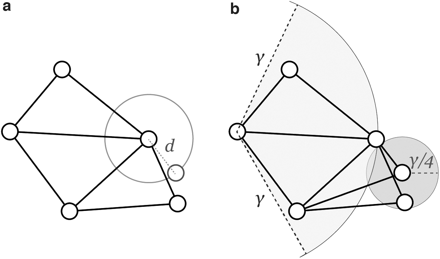
A diagram demonstrating the mutation of a node and the new connections formed with the regenerated node. (a) Shows a new node spawning off of an existing node in a random direction, with a displacement of d. (b) Shows this new node and its new connections made with existing nodes. The maximum distance between new connections is denoted with $γ$ , which is the maximum distance used during lattice initialization. The minimum distance between new connections is denoted with $γ ∕ 4$ .

After creating a new lattice state L_i, we run the culling algorithm until the mass criteria has been satisfied again, followed by another run of the strut regeneration search. This process repeats iteratively until the deflection criteria is also satisfied.

Results

We present several examples below demonstrating the outcome of our method on various load types. See Equation (1) for example structures that have been fabricated. This section will begin by covering the results of the strut removal process on static and dynamic load cases.

Strut removal method

Strut removal runs in a straightforward manner on static objects. At each iteration the simulation reanalyzes the stress values for each strut and determines which struts to remove, which continues until a user-defined stop criterion is met. We show a static example of a table optimization, where the four bottom corners of the design space are fixed, as posts, and a downward force is distributed across the top surface (Fig. 4). The table is high voxel resolution, with 235K struts in the initialization, which is generated through the cubic overlay method. In the figure, it is clear that a heterogeneous microstructural pattern has formed.

FIG. 4.

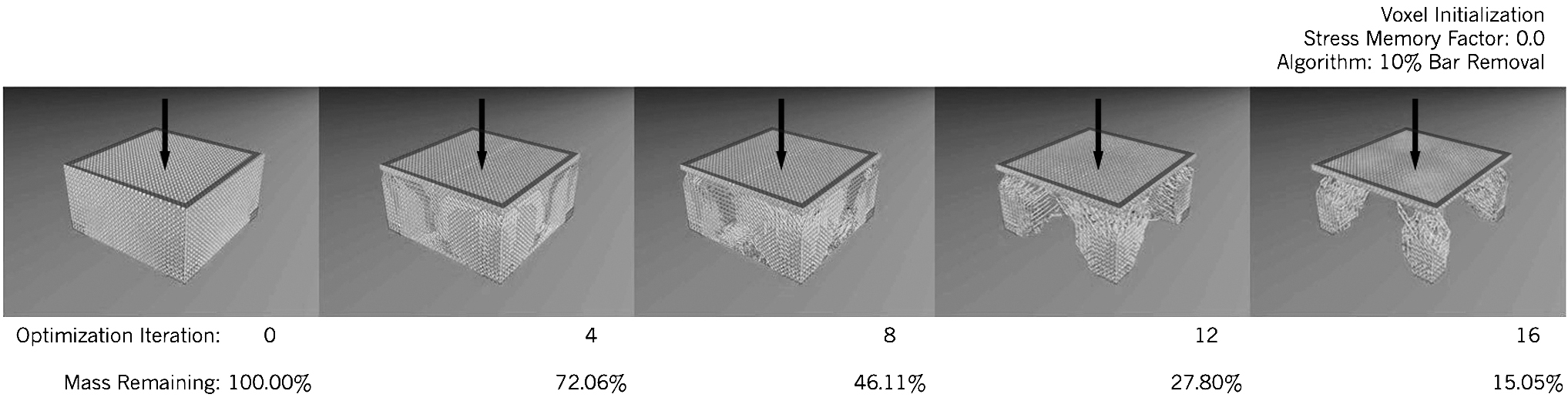
Progression of the 10% parallel algorithm on a top-loaded table example with four base anchors and a contact floor. Note that “Mass Remaining” refers to the mass culled from the starting lattice initialization, which begins with already diminished mass from the full design volume.

Strut removal on dynamic objects

Because optimization is run simultaneously with simulation, optimization can be configured on dynamic physical systems as well as static ones. The kinematics of a mass–spring system are calculated during the same integration process as relaxation. Thus, collisions are simulated real-time, and we can analyze the maximum stress of each strut in a similar way to static loads. Dynamic load cases vary over time, thus which parts of the object that are necessary will vary as well. Because maximum stress is stored continuously as a property of each strut, the stress comparison across struts at any point in time is impacted by the entire history of the simulation. We address this with a stress memory factor, which we use to modulate the time that stress values are stored on each strut. We go into further detail about stress memory below.

To test our algorithm on dynamic load cases, we used an example of a bouncing cube. The cube was initialized with a quasi-uniform random lattice with side lengths of 10 cm. It was set to fall from a height of 20 cm onto a contact plane. Note that a single drop creates an asymmetrical stress pattern: the face of the cube touching the plane incurs a greater amount of external force than the rest of the cube. The final target structure was one that might act as a thrown die: any face or corner should be able to hit the plane and the integrity of the volume should remain intact. Thus, the simulated scenario was set to test multiple orientations of the cube, dropping the “die” for multiple rolls. In between drops, the center of mass of the cube was reset to its initial position with a random 3D rotation. The cube was bounced 20 times before optimization began to accrue a coherent stress pattern. See Figure 1 for a 3D printed cross-section of the resulting cube.

Removing struts in parallel

To achieve real-time optimization speed even on large structures, a “culling” factor was introduced such that a percentage of struts might be removed every iteration. This dramatically sped up the mass removal process and scaled to high-resolution structures. Several magnitudes were tested for success of the parallel removal algorithm, which were then compared with the single-strut removal algorithm.

Based on the comparison shown in Table 1, the parallel removal algorithms speed up the technique with increasing magnitude as parallelism increases. The times represent the entire simulation and optimization process, achieving speeds well high enough to incorporate user interaction for testing different constraint arrangements.

Table 1.

Speeds of Several Magnitudes for the Strut Removal Algorithm on a Beam with a Pseudo-Random Lattice of About 3K Struts

Magnitude (struts)	Time to 50% mass (s)
Single	892.91
1%	42.84
5%	9.18
10%	4.90
20%	3.06

The relaxation interval between iterations is 5 × 10⁵ dt, with $d t = 1 \times 1 0^{- 6} s$ .

For measuring success, we used a mass against deflection metric. Mass was calculated according to lattice geometry and material density. Deflection was chosen as the average movement of point masses with non-zero external force vectors from their original positions. On the cantilever beam example for instance, deflection was calculated from the loaded tip of the beam.

Deflection is calculated slightly differently for dynamic load cases. Because there is no static external load, deflection is computed as such: $δ = Σ_{i = 0}^{i < a} | | X_{0} - Y_{0} | | - | | X_{i} - Y_{i} | |$ , where X is the initial position of a mass and Y is the position at any future state, and X₀ and Y₀ denote the initial and current positions of the center of mass of the system. We normalize the deflection measurement against the center of mass to account for translation and rotation of the structure as a whole.

We compare the different speed algorithms with another comparison of Pareto fronts between mass and deflection (Fig. 5). Note that the static case, the beam example, shows comparable success between the single strut removal algorithm and low-percentage parallel removal algorithms. However, when the algorithm is extended to 20% strut removal, the success of the algorithm degrades as we see a totally subsumed Pareto front.

FIG. 5.

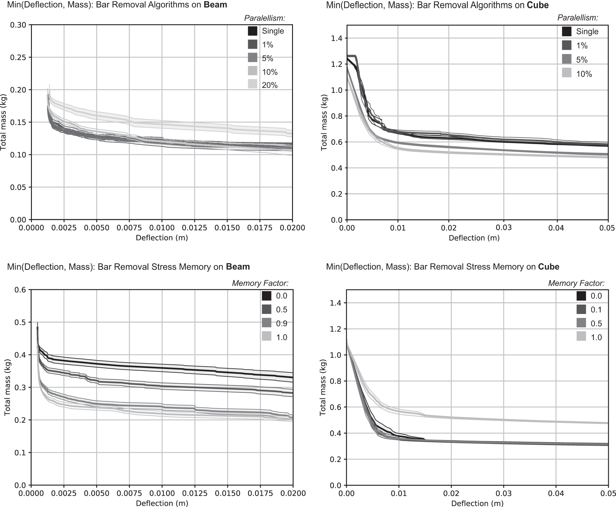
Pareto fronts for top left: various strut removal algorithms on a cantilever beam of mass versus deflection. (Top right): various strut removal algorithms on a dynamic bouncing cube of mass versus deflection. (Bottom left): various stress memory factors on a cantilever beam of mass versus deflection. (Bottom right): various stress memory factors on a dynamic bouncing cube of mass versus deflection. The beam has 41K struts in the initialization, and the cube has 79K struts in the initialization.

For the dynamic bounding cube example, the algorithms of higher parallelism subsume those of lower parallelism (Fig. 5). This phenomenon is likely caused by the repeat methodology in the initialization of this example. The cube is bounced 20 times at the start and then, at a resting state, is optimized. This is to ensure stress symmetry for all sides and corners of the cube. This occurrence will likely vary under different dynamic examples that use different arrangements for repeating a dynamic load.

Stress memory

Another property that we varied and tested in our algorithm was stress memory, the amount of past stress each strut retains in its lifetime. To vary this property, we define a stress memory factor between 0.0 and 1.0, which is multiplied with the strut maximum stress values after every optimization iteration. Thus, we can reset all of the maximum experienced stresses between every optimization iteration with a factor of 0.0. Or, we can retain all of the maximum experienced stress throughout the entire simulation with a factor of 1.0. We compare these values in Pareto fronts on the cantilever beam and bouncing cube examples. Figure 5 shows the results of different stress memory factors.

The static example shows that the success of the algorithm is greater when the stress memory factor is higher. This demonstrates that the retention of the maximum stress value across the entire simulation is relevant in static examples. Thus, past states of the beam inform a better solution for future states. However, on the dynamic cube example we see a reversal where the 1.0 memory factor performed the worst. In this study, a small (but existent) memory factor appears to create the best structures, with 0.1 and 0.9 competing with 0.0 for the superior front. As past bounces become increasingly irrelevant, it is in the algorithm's interest to “forget” older stress metrics.

Strut regeneration and removal

We subsequently tested the optimization containing both strut removal and regeneration. This process is illustrated in Figure 6, where the progression of the simulation with these two optimization methods running is shown. After an hour, the beam achieves a deflection of 17% the original.

FIG. 6.

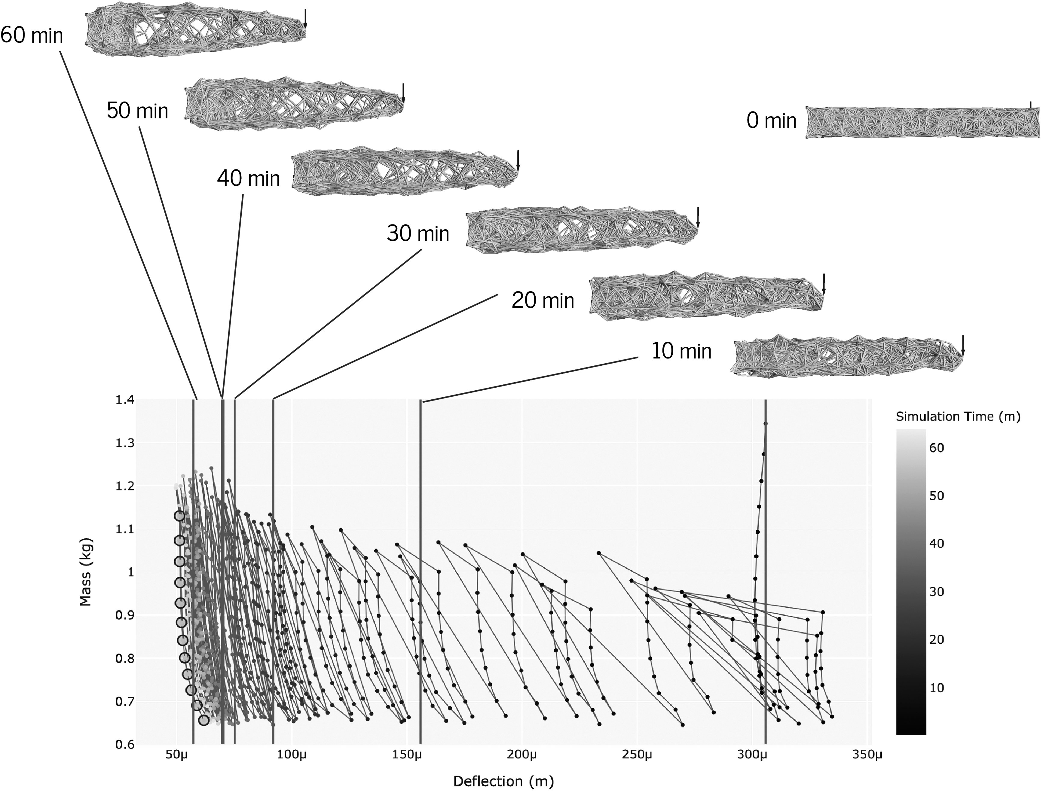
A graph showing the progression of the strut regeneration and removal optimization running on a cantilever beam lattice for 72 total iterations of the algorithm. As time increases, the chart moves from the right to left with deflection. Each strut removal and regeneration step are shown as a point. Each regeneration iteration can also be recognized in the sharp increases in mass after a series of removal steps. The last run of strut removal iterations is shown on the left in orange. The beam is initialized with the quasi-random lattice generation. Every 10 min of the simulation is marked with a vertical line, and the resulting lattice at that point is shown above.

The figure demonstrates some interesting properties of this optimization. As shown in the initial run, strut removal can decrease deflection as well as mass occasionally, as shown by the slight curvature in some of the removal series. This is because struts near the load can weigh down the lattice without providing any structural benefit. Thus, once they are removed, the lattice improves on both criteria. In addition, the progression of the algorithm is faster at first, with the deflection decreasing 50% in the first 10 min. As the optimization continues, gains in the optimization criteria take longer, but we do see more vivid structural changes during this time. Finally, the total mass of the lattice increases from each previous strut regeneration with each new one (note that the total mass of the structure remains constant once each full run of strut removal follows). This is because the metric used by the authors to regenerate struts was based on the number of existing struts, rather than the existing total mass. This phenomenon does not affect the success of the algorithm because culling uses a mass-based metric.

Furthermore, our nonmodified strut regeneration algorithm does not impose volume constraints on the design space. Therefore, the resulting structure grows past its original volume to find a more optimal shape. See the GE Bracket Case Study for more results from the volume-bounded variation of this algorithm.

The parameters used for this optimization were a 5% culling rate (the percentage of strut removed each iteration), a 10% regeneration rate (the percentage of existing struts to be generated each iteration), and a 50% regeneration trigger (the percentage of remaining mass after a series of strut removals at which to trigger a regeneration iteration).

A more complete run of the regeneration optimization on a cantilever in shown in Figure 7. The beam parameters are identical to that in Figure 6, but uses a different random seed for lattice initialization.

FIG. 7.

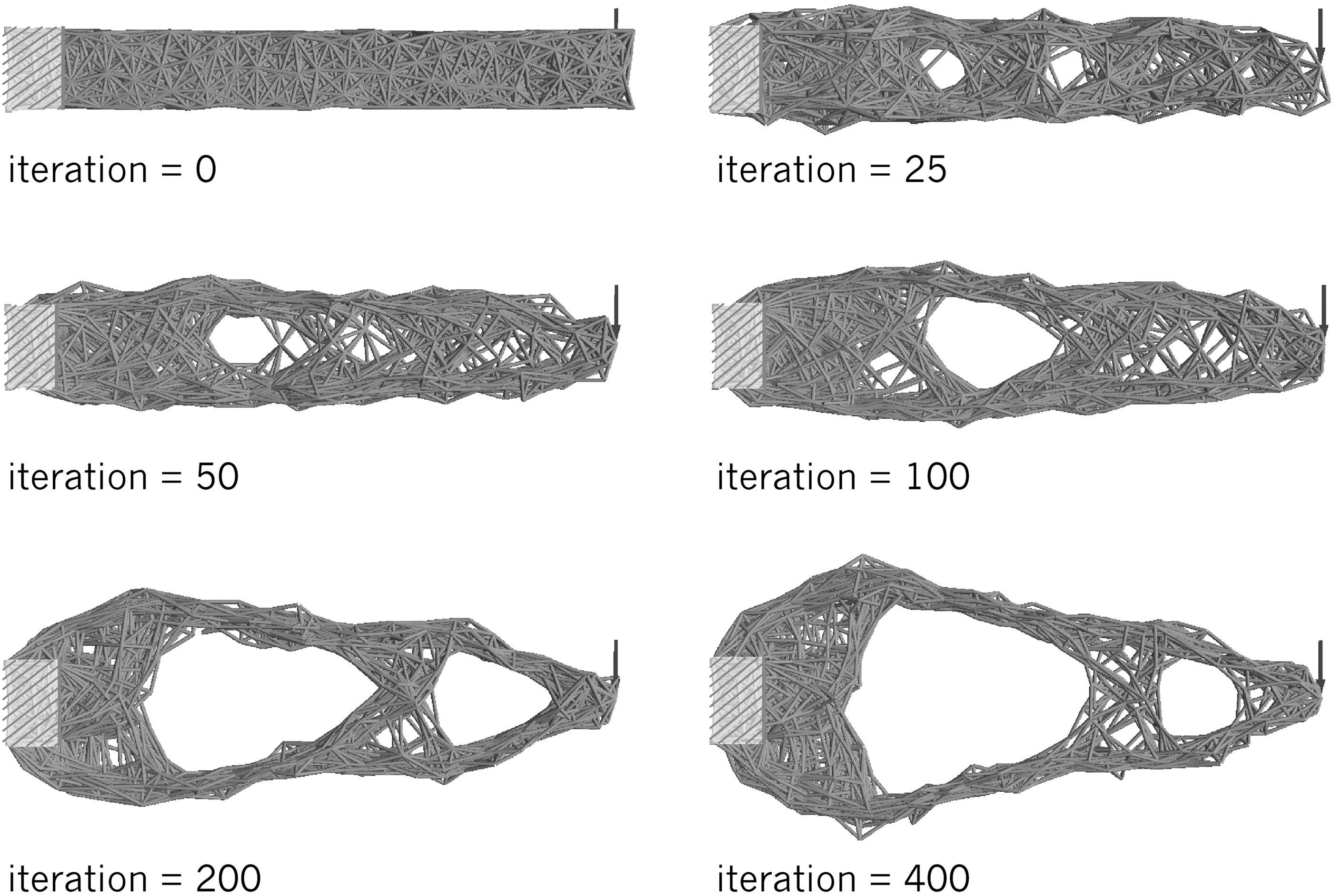
A diagram illustrating a long run of the material regeneration and removal algorithm on a cantilever beam initialized with a quasi-random lattice. Each iteration refers to a regeneration step.

Testing regeneration parameters

To give a sense of suitable parameters for our regeneration method, we tested different values of three optimization parameters on our cantilever beam example: (1) culling rate, (2) regeneration amount, and (3) regeneration mass trigger. Figure 8 shows the results of these tests. This run took a little over 15 h on a Titan X GPU.

FIG. 8.

Three graphs each comparing a different parameter's values over multiple trials on a cantilever beam with constant mass: (a) culling rate, (b) regeneration amount, and (c) regeneration trigger. The graphs on the left show the given simulation's deflection over time, with standard error across trials. Each graph compares between three and five different parameter values. The bar graphs on the right show a snapshot of each parameter value after a 30-min run. The error here shows variance over the prior 5 min.

We ran 6 trials per parameter value for 50 regeneration iterations (for the line graphs). The results of the culling rate testing show that a lower culling rate (see 1%) results in a stable optimization but a longer wall clock time, while a higher culling rate (see 15%) results in a more volatile optimization curve but a much faster speed, clocking in at nearly 10 × faster than the 1% results. A 5% culling rate offers a helpful medium, where time variance is low but the optimization is still performed relatively quickly. This is supported by the associated deflection snapshot bar graph, where 5% and 15% culling rates achieve similar deflection reduction, with the error bar capturing the higher variance for 15%. We also graphed the results for a 4% and 6% culling rate, which follow the same pattern described above.

The results for the regeneration amount tests support that a regeneration rate of 10% or above is recommended as the pool of new struts is larger for each iteration. The comparison graphs show that this is the case as the 10% and 15% regeneration amounts optimize slightly faster at the 30-min mark. However, this difference is not large enough to be statistically significant.

We finally tested the regeneration trigger point, at which percentage of our original mass do we stop removing material, and perform another regeneration. Here we find that higher mass triggers result in lower volatility and higher success. It is worth noting that this regeneration trigger controls the final weight reduction of the structure as the lower bound. Thus, it is expected that higher mass final structures result in lower deflections. This tradeoff will be determined by the users' requirements for their output structure.

Performance comparison

Case study: GE Bracket Challenge

A study was performed to assess the performance of the optimized lattice structure with a known design and load-case optimization, the GE Bracket Challenge.²⁴ We generated two distinct optimized lattice designs with the strut removal and regeneration methods. We included a volume constraint in the regeneration method, as this condition is necessary for the case study, but not inherent to the method. Figure 9 shows the structure with the volume-bounded regeneration technique. The resulting lattice structures were then postprocessed in nTopology to retain the loading and fixture points, and the resulting design analysis was performed with the load cases from the GE Bracket Challenge, using a combination of FE Tet and Beam elements with tie constraints to bond the lattice structure to the fixture points. Convergence studies were done with both the sizing of the Tet elements and Beam element subdivisions to determine the appropriate parameter set and confirm results. The first- and second-place challenge winner designs were also assessed with the same FE Model as previously described, without the Beam elements and tie constraints (which were not necessary for the solid body designs). Another case study is available in Appendix C that uses a simpler design space, but provides an additional comparison.

FIG. 9.

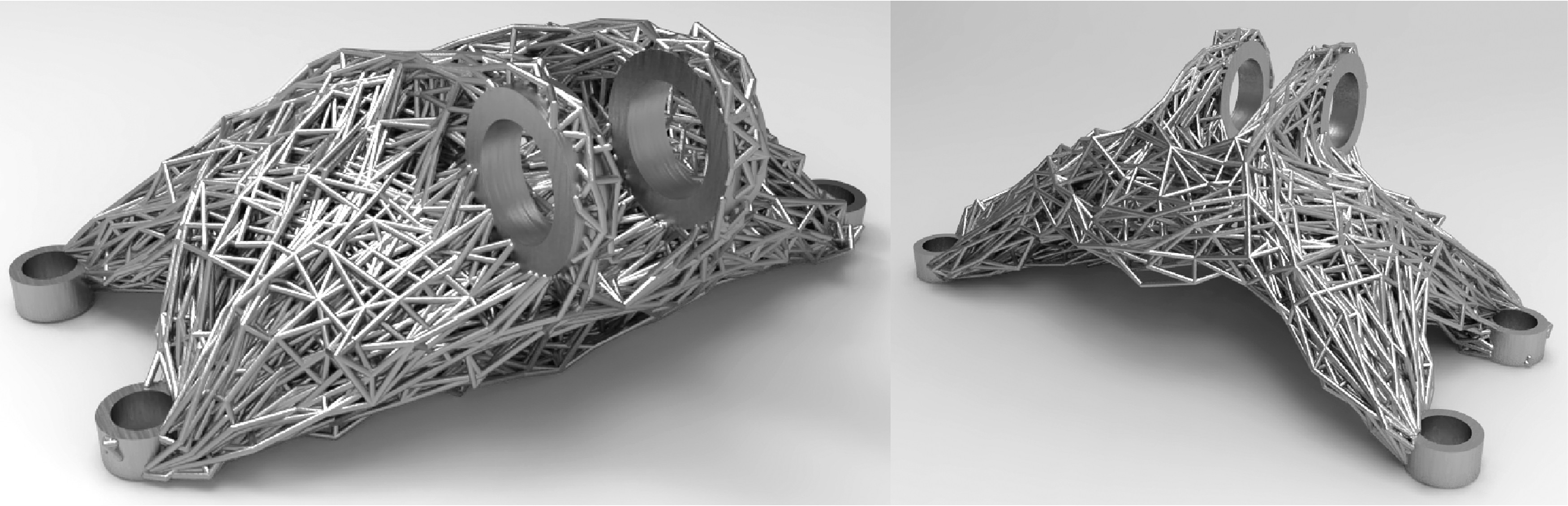
High resolution render of the final analysis geometry, with lattice generated from strut regeneration method with a volume constraint. (Left) Front view. (Right) Back view.

Many iterations were performed with both the volume-bounded regeneration and strut removal methods, along with iterations for single load optimization of all three major loads from the GE Bracket Challenge as well as a multiload optimization for all three major loads (the three major loads being defined as loads 1, 2, and 3—excluding the torque case). The resulting structures were then postprocessed to adequately define all mounting points.

The resulting structures' performance was simulated with the nTopology Platform to gain a sense of the lattice performance compared with the solid body optimizations that were submitted to the GE Bracket Challenge. Figure 10 shows that our optimized lattice structures were able to match, and in some cases outperform the mass/deflection performance of the GE Bracket Challenge winners while retaining the fact that it is a semi-hollow architected material structure rather than a solid body optimization. The results of these comparisons for the three major load cases are pictured.

FIG. 10.

Mass versus deflection performance charts comparing our method against the winners of the GE Bracket Challenge.²⁴

On all three major loads, the strut removal method is able to perform similarly to the solid body optimization results (the winners of the GE Bracket Challenge). It is notable that with our strut regeneration method, where we include a volume constraint, we are able to improve the performance significantly such that it outperforms the competitor designs in all three load cases.

Limitations and future work

We recognize that our technique has many avenues for further development and improvement. For instance, our model comes with several limitations when the results are transferred to real-world fabrication. Primarily we model the lattice strut connections as pin joints rather than welded joints. Furthermore, our simulation assumes isotropic materials, while many AM techniques produce anisotropic results from the layering process. The relaxation method does not account for other nonlinear effects, i.e., thermal, buckling, and other physical phenomena. We also primarily used a weight-based target, and thus our technique requires further analysis on different optimization criteria. A particular challenge is the time needed for relaxation as a function of the number of struts and specifics of the geometry: less compact structures take longer to relax. Similarly adaptive relaxation and optimization schedules could be explored. These will be incorporated in future. We acknowledge that further work is required to validate this for robustness across a wider variety of physical designs.

In validation, we note several areas of improvement for our lattice simulation technique. Our method does not account for overlaps between beams with small angles stemming from the same mass origin. Additionally, it does not account for intersections between beams with no shared masses. To improve upon this, it would be ideal to break intersections such that a new mass is created at the junction of the beams.

Further work needs to be done to determine the most viable method for validating these lattice structures. While the NTLatticeGraph method allows for much faster processing of the lattice structures, we showed that due to the lack of accounting for intersection and overlap, the results artificially strengthen the part. Altering the lattice graph to account for intersections could improve this. Conversely, the finite element tetrahedral mesh method quickly becomes extremely computationally expensive when working with complex lattices, and requires a very precise mesh sizing to properly preserve the part geometry.

Conclusion

In this article, we have presented a technique for the simulation and structural optimization of complex lattice structures. This includes the contribution of simultaneous simulation and optimization, allowing for a variety of optimization operations to occur iteratively. In this work, we have presented the combination of two operations: strut removal and regeneration. We have validated our results against existing topology optimization systems. We demonstrate that a lattice-based technique that operates locally can achieve a fine structure that is difficult to create through traditional methods, along with comparable performance results.

The code used to generate the results in this article is fully open source, and can be found at github.com/swyetzner/dml-ide .

Footnotes

Author Disclosure Statement

No competing financial interests exist.

Funding Information

This work has been funded in part by U.S. Defense Advanced Research Project Agency (DARPA) TRADES grant number HR0011-17-2-0014.

Supplementary Material

References

Bendsøe

, Kikuchi

. Generating optimal topologies in structural design using a homogenization method. Comput Methods Appl Mech Eng, 1988; 71:197–224.

Doubrovski

, VerlindenJC, Geraedts

. Optimal design for additive manufacturing: Opportunities and challenges. In: ASME 2011 international design engineering technical conferences and computers and information in engineering conference. American Society of Mechanical Engineers, 2011; pp. 635–646.

Liu

, Gaynor

, Chen S et al. Current and future trends in topology optimization for additive manufacturing. Struct Multidisc Optim, 2018; 57:2457–2483.

Sigmund

, Maute

. Topology optimization approaches. Struct Multidisc Optim, 2013; 48:1031–1055.

Liu

, Hu

, ZhuB, et al. Narrow-band topology optimization on a Sparsely Populated Grid. ACM Trans Graph, 2018; 37:251:1–251:14.

Aage

, Andreassen

, Lazarov

, et al. Giga-voxel computational morphogenesis for structural design. Nature, 2017; 550:84.

Baandrup

, Sigmund

, Polk

, et al. Closing the gap towards super-long suspension bridges using computational morphogenesis. Nat Commun, 2020; 11:2735.

, Dick

, Westermann

. A system for high-resolution topology optimization. IEEE Trans Vis Comput Graph, 2015; 22:1195–1208.

Austin

, Corrales-Fatou

, Wyetzner

, et al. Titan: A parallel asynchronous library for multi-agent and soft-body robotics using NVIDIA CUDA. In 2020 IEEE International Conference on Robotics and Automation (ICRA), Paris, France, 2020; pp. 7754–7760.

10.

Zegard

, Paulino

. GRAND—Ground structure based topology optimization for arbitrary 2D domains using MATLAB. Struct Multidisc Optim, 2014; 50:861–882.

11.

Zegard

, Paulino

. GRAND3—Ground structure based topology optimization for arbitrary 3D domains using MATLAB. Struct Multidisc Optim, 2015; 52:1161–1184.

12.

Wang

, Tai

. Bar-system representation for topology optimization using genetic algorithms. Eng Comput Bradf, 2005; 22:206–231.

13.

Ahmed

, Deb

, Bhattacharya

. Structural topology optimization using multi-objective genetic algorithm with constructive solid geometry representation. Appl Soft Comput, 2016; 39:240–250.

14.

Norato

, Bell

, Tortorelli

. A geometry projection method for continuum-based topology optimization with discrete elements. Comput Methods Appl Mech Eng, 2015; 293:306–327.

15.

Sigmund

, Aage

, Andreassen

. On the (non-)optimality of Michell structures. Struct Multidisc Optim, 2016; 54:361–373.

16.

Michell

AGM

. LVIII. The limits of economy of material in frame-structures. Philos Mag J Sci, 1904; 8:589–597.

17.

Sokól

. A 99 line code for discretized Michell truss optimization written in Mathematica. Struct Multidiscip Optim, 2011; 43:181–190.

18.

Arora

, Jacobson

, Langlois

, et al. Volumetric Michell trusses for parametric design & fabrication. In Proceedings of the ACM Symposium on Computational Fabrication, ACM, Pittsburgh, PA, 6, 2019.

19.

Rozvany

. Some shortcomings in Michell's truss theory. Struct Optim, 1996; 12:244–250.

20.

Stolpe

. Truss optimization with discrete design variables: A critical review. Struct Multidiscip Optim, 2016; 53:349–374.

21.

Gutkowski

, Bauer

, Zawidzka

. An effective method for discrete structural optimization. Eng Comput, 2000; 17:417–426.

22.

Southwell

RV.

Relaxation Methods in Engineering Science. Oxford, England: Oxford University Press, 1940.

23.

Smith

, Hodgins

, Oppenheim

, et al. Creating models of truss structures with optimization. ACM Trans Graph, 2002; 21:295–301.

24.

GE jet engine bracket challenge | Engineering & Design Challenges | GrabCAD. https://grabcad.com/challenges/ge-jet-engine-bracket-challenge (accessed January 27, 2020).

25.

Mitchell

. Spectrally optimal sampling for distribution ray tracing. ACM Siggraph Comput Graphics, 1991; 25:157–164.

Supplementary Material

Please find the following supplemental material available below.

For Open Access articles published under a Creative Commons License, all supplemental material carries the same license as the article it is associated with.

For non-Open Access articles published, all supplemental material carries a non-exclusive license, and permission requests for re-use of supplemental material or any part of supplemental material shall be sent directly to the copyright owner as specified in the copyright notice associated with the article.

0.00 MB

0.05 MB

0.01 MB