Investigation of Obstacles with Interactive Elements on the Flow in SiC Three-Dimensional Printing

Abstract

A single screw extruder is used in this study to efficiently transport SiC slurry in direct ink writing (DIW) technology. The deposits caused by low viscosity and the agglomerations resulting from the nonuniform mixing form the obstacles in the channel, which affect the normal flow of the slurry, theoretical outlet velocity, and interaction with other printing parameters. Therefore, it is necessary to study the effect mechanism of the obstacles on the flow. The obstacles are always irregular, which makes it difficult to directly analyze them. Irregular geometries are always composed of linear and/or arcuate elements; therefore, the obstacles can be simplified into regular geometries. In the present work, interactive elements, including line–line, line–arc, arc–arc situations are analyzed. Then, an improved multiple relaxation time lattice Boltzmann method (MRT LBM) with a pseudo external force is proposed for the flow analysis. The improved MRT LBM is combined with rheological test data to investigate cases with interactive elements, and the results are applied to reveal the general mechanism. The results show that the positions are common influencing factors, which affect the streamlines, outflow directions, and outlet velocity distributions. In addition, in different situations, different factors are considered to affect SiC slurry flow. It is obvious that the existed obstacles inevitably change the theoretical flow direction and outlet velocity, which has a synergistic effect on the printing parameters. It is necessary to understand the effect mechanism of the obstacles on the flow.

Introduction

Ceramic materials have many excellent properties, such as high melting points, hardness, and stability, and they have been applied in the aerospace, biology medicine, consumer electronics, and mechanical manufacturing areas.^1–4 However, the complex structure of ceramic parts and hardness of the materials make them difficult to form successfully by traditional molding methods. A new type of intelligent manufacturing technology, additive manufacturing, provides another effective method for forming ceramic parts.^5–9 Direct ink writing (DIW) technology can easily form most kinds of ceramic materials with complex structures.^10–14

Regarding DIW technology, excellent flowability is expected, whereas SiC slurry has a low viscosity. To improve the transportation performance, the single screw extruder is adopted here. In the transportation process, the uniform and smooth fluid contribute to obtaining perfect printing properties for the parts. However, the viscous slurry may deposit gradually, and the nonuniform mixing leads to agglomerations, both of which can be viewed as obstacles in the flow channel. The obstacles directly affect the streamlines and velocity of the flow. Therefore, it is crucial to understand the mechanism responsible for the effects of the potential obstacles.

The referred analysis belongs to the computational fluid dynamic case. Many numerical methods can be used to solve the flows, such as the finite element method^15,16 and finite volume method.^17,18 The Fluent software is developed based on the above methods, which is applied in some non-Newtonian flow cases. Pantokratoras A simulated power-law fluid flow in a square section by using Fluent.¹⁹ Husain et al. conducted numerical analyses to investigate the effect of geometrical parameters on the natural convection of water in a narrow annulus, where the fluids belong to power-law type.²⁰ Zhou and Bayazitoglu analyzed the heat transfer for power-law fluids between two parallel plates.²¹ Kumar et al. analyzed the heat transfer of power-law fluids in a semicircular cylinder.²² Although it is convenient to conduct the flow analysis by using Fluent, the complex types of non-Newtonian fluids cannot be satisfied and additional secondary development is always required. In contrast, lattice Boltzmann method (LBM) is a mesoscopic computational method, which achieves the flow analysis by calculating given equations iteratively.

The calculation is easy to implement by Visual C, Fortran, and MATLAB. Regarding the non-Newtonian fluid flow, much research has been done. Kefayati and Huilgol simulated the Bingham flow in a pipe by a modified lattice Boltzmann (LB) model.²³ Zhang et al. conducted free-surface simulations of Newtonian and Bingham fluid flow with LBM, and a mass tracking model is used to capture the free surface.²⁴ Khabazi et al. studied Bingham flow with large Reynolds numbers by using LBM.²⁵ The abovementioned LBM is also named as the single relaxation time LBM, while the multirelaxation time LBM is developed to improve some other performances such as stability. Wu, et al. introduced a universal modified multiple relaxation time lattice Boltzmann (MRT LB) model for non-Newtonian fluid flow, where the power-law, Bingham, and Herschel–Bulkley types are explored carefully.²⁶ Qiu and Han applied three-dimensional multiple relaxation time lattice Boltzmann method (MRT LBM) in analyzing self-compacting concrete flow, which is viewed as non-Newtonian fluids.²⁷

Yang and Wang investigated the power-law flow in rectangular enclosures to reveal the effects of magnetic field on the flow, which is simulated by MRT LBM.²⁸ Molla et al. developed a modified power-law equation to simulate the flow based on MRT LBM.²⁹ Sajjadi et al. proposed a new double MRT LBM to analyze magnetohydrodynamics natural convection in a porous media.³⁰ It is found that LBM is an effective method in solving non-Newtonian fluid flow, including macroscopic and microscopic scales. Some modified models are proposed to further improve the stability or accuracy of the simulation because of the changeable viscosity in each iteration. Based on the rheological behavior of the mixing slurry in the current work, MRT LBM is adopted to implement the flow analysis by using MATLAB software.

The article is organized as follows. In Rheological Behavior section, the rheological behavior of SiC slurry is tested, and a rheological equation is built. In Pseudo-External-Forced MRT LBM for Non-Newtonian Ceramics Flow section, the MRT LBM with a pseudo external force is proposed and validated by the classical cases. In Effects of Multiple Linear Obstacles on the Flow of Ceramic Slurry section, some cases are analyzed, and the simulation results are obtained. Finally, the effect mechanism is discussed and conclusions are drawn in Discussion and Conclusion sections, respectively, which will contribute to understanding actual slurry flows in extruders.

Rheological Behavior

Preparation

The raw materials are listed in Table 1, where polyvinyl alcohol is worked as the binder. The polyvinyl alcohol is mixed uniformly with water to obtain the binder solution. Then, the other powders are added to the solution and fully dissolved by centrifugation at 1000 rpm for 3 min. In this way, the SiC slurry with 80 wt. % solid content can be obtained.

Table 1.

The Used Raw Materials

Material	Average particle size	Weight percentage
SiC ceramic powders	0.5 μm	60
Carbon powders	250 nm	20
Polyvinyl alcohol	—	5
Water	—	20

Rheological test and result

The rheological performance is required to investigate for the following computational fluid dynamic analysis. An AR2000 EX rheometer is used here and the SiC slurry is presheared at a shear rate of 10 s⁻¹ for 5 s. Then, the viscosity is measured by increasing the shear rate from 0.1 to 1000 s⁻¹ at a frequency of 1 Hz. The obtained viscosity curve is shown in Figure 1.

FIG. 1.

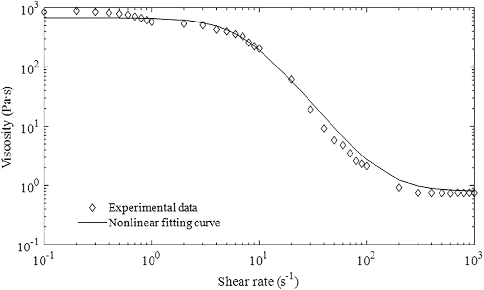
Experimental rheology data and nonlinear fitting results.

In Figure 1, the experimental results described by the discrete points show that the slurry exhibits non-Newtonian characteristics. The curves of common types of non-Newtonian fluids are used to compare with the experimental data, and the results indicate that rheology data can be closely fitted with the Carreau model. The specific rheological equation of the Carreau model is expressed as follows:

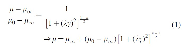
where μ is the dynamic viscosity, μ₀ and μ_∞ are the viscosities at zero and infinite shear rates, respectively, λ is the time constant, $\dot{γ}$ is the shear rate, and n is the power-law index. The fitting process is calculated by MATLAB, and the specific results are given as: μ₀ is 678.1 Pa·s, μ_∞ is 0.8 Pa·s, λ is 0.1464 s, and n is −1.18. Thus, the specific rheological equation of the SiC slurry is: $μ = 0.8 + 677.3 {[1 + {(0.1464 γ)}^{2}]}^{- 1.09}$ (2)

In Figure 1, the curve implies that three zones exist in the shearing process: the curves in the first and the third ranges are almost horizontal, where the slurry can be viewed as Newtonian fluids, and the corresponding ranges of shear rates are [0, 10 s⁻¹] and [110, 1000 s⁻¹], respectively. In the second zone, whose range of shear rate is (10, 110 s⁻¹), the viscosity presents typical non-Newtonian behavior, which decreases rapidly with increasing shear rate.

Pseudo-External-Forced MRT LBM for Non-Newtonian Ceramics Flow

Specific method

When MRT LBM is used to solve the non-Newtonian problems, divergence or poor accuracy may occur because the viscosity varies for different shear rates. To improve the non-Newtonian flow analysis, a pseudo external force method is introduced based on the MRT LBM. According to the LB model, including the forcing term proposed by Guo et al.,³¹ the MRT LBM, including the forcing term, can be obtained as follows: $\begin{matrix} f (r + e_{i} δ t, t + δ t) - f (r, t) & = - M^{- 1} \bar{S} M [f (r, t) - f^{e q} (r, t)] \\ + δ t F' \end{matrix}$ (3)

where the discrete lattice forcing term F′ is expressed as: $F^{'} = M^{- 1} (I - \frac{\bar{S}}{2}) M \bar{F}$ (4)

and where M is a transformation matrix as follows: $M = (\begin{matrix} 1 & 1 & 1 & 1 & 1 & 1 & 1 & 1 & 1 \\ - 4 & - 1 & - 1 & - 1 - & 1 & 2 & 2 & 2 & 2 \\ 4 & - 2 & - 2 & - 2 & - 2 & 1 & 1 & 1 & 1 \\ 0 & 1 & 0 & - 1 & 0 & 1 & - 1 & - 1 & 1 \\ 0 & - 2 & 0 & 2 & 0 & 1 & - 1 & - 1 & 1 \\ 0 & 0 & 1 & 0 & - 1 & 1 & 1 & - 1 & - 1 \\ 0 & 0 & - 2 & 0 & 2 & 1 & 1 & - 1 & - 1 \\ 0 & 1 & - 1 & 1 & - 1 & 0 & 0 & 0 & 0 \\ 0 & 0 & 0 & 0 & 0 & 1 & - 1 & 1 & - 1 \end{matrix})$ (5)

$\bar{S}$ is a diagonal matrix associated with the relaxation process, whose detailed expression is: $\bar{S} = d i a g (0, s_{e}, s_{δ}, 0, s_{q}, 0, s_{q}, s_{ν}, s_{ν})$ (6)

where s_e is relevant to the viscosity, which is set to 0.8. s_ɛ is a parameter to control the stability of the simulation, which is set to 0.8. s_q affects the accuracy of the model, which is defined as 1.9. s_ν is equivalent to the standard single relaxation time LBM. With expanding the Chapman–Enskog equation, the Navier–Stokes equation at the incompressible limit can be recovered as follows: $\begin{matrix} ρ \partial_{t} (u_{β}) + (ρ u_{α}) \partial_{α} u_{β} = - \partial_{β} P + 2 λ \partial_{α} S_{α β} \\ + 2 [μ_{\infty} + (μ_{0} - μ_{\infty}) {[1 + {(λ γ)}^{2}]}^{\frac{n}{2}} - λ] \partial_{α} S_{α β} \\ = - \partial_{β} P + 2 λ \partial_{α} S_{α β} + \bar{F} \end{matrix}$ (7)

For Carreau fluids, the external force-related term $\bar{F}$ is expressed as follows: $\bar{F} = 2 [μ_{\infty} + (μ_{0} - μ_{\infty}) {[1 + {(λ γ)}^{2}]}^{\frac{n}{2}} - λ] \partial_{α} S_{α β}$ (8)

According to Equations (4) and (8), the discrete lattice force term F′ for Carreau fluids can be further calculated as follows: $\begin{matrix} F_{i}^{'} & = 2 ω_{i} (1 - \frac{δ t}{τ}) [\frac{e_{i} - u}{c_{s}^{2}} + \frac{e_{i} \cdot u}{c_{s}^{4}} \cdot e_{i}] \\ [μ_{\infty} + (μ_{0} - μ_{\infty}) {[1 + {(λ γ)}^{2}]}^{\frac{n}{2}} - λ] \partial_{α} S_{α β} \end{matrix}$ (9)

By substituting Equation (9) into Equation (3), the non-Newtonian behavior is treated as a pseudo external force.

MATLAB is used to conduct the fluid flow simulations. The specific calculation steps can be referenced as follows.

(S1) Unit conversion: The Reynolds number, Mach number can be used as the criterion to transform the physical quantities into dimensionless parameters for MRT LBM. In the current work, the Reynolds number is selected to implement the unit conversion.

(S2) Initial definition: Some essential parameters should be defined firstly, such as the lattice numbers, the initial viscosity, the dimensionless density, and the driven pressure or inlet velocity. The inlet velocity is given to drive the flow in the current work.

(S3) Distribution functions definition: The distribution functions mentioned here include two parts: the initial and equilibrium functions. Commonly, they can be set as the same one as follows:

f^{e q} (r, t) = ω_{i} ρ [1 + \frac{e_{i} \cdot u}{c_{s}^{2}} + \frac{{(e_{i} \cdot u)}^{2}}{2 c_{s}^{4}} - \frac{u^{2}}{2 c_{s}^{2}}]

(10)

where the weight coefficient ω_i is set as ω₀ = 4/9 for i = 0, ω_i = 1/9 for i = 1–4, and ω_i = 1/36 for i = 5–8. c_s is the lattice sound speed, which is described as $c_{s}^{2} = c^{2} ∕ 3 = {(δ x ∕ δ t)}^{2} ∕ 3$ . δx is the lattice step distance, which is always set as 1. δt is the lattice time, which is also set as 1. u is the velocity. e_i is the discrete velocity parameter, which is expressed as follows: $e_{i} = \{\begin{matrix} (0, 0), i = 0 \\ c (cos \frac{i - 1}{2} π, sin \frac{i - 1}{2} π), i = 1, 2, 3, 4 \\ \sqrt{2} c (cos \frac{2 i - 9}{4} π, sin \frac{2 i - 9}{4} π), i = 5, 6, 7, 8 \end{matrix}$ (11)

(S4) Streaming and collision actions: Two parts can use a synthesis function as shown in Equation (3), where the pseudo external force is used to describe the non-Newtonian behavior of the slurry. The specific expression is expressed as Equation (9).

(S5) New parameters’ calculation: When the above steps are finished, the new relaxation parameters should be calculated for the following iterations.

(S6) Boundary processing: Concerning the LB calculation, many classical boundary processing methods have been proposed. In the current work, the non-equilibrium bounce-back method is adopted.

(S7) Error calculation: The relative error is set to judge whether the simulation has been finished. According to the different accuracies, a sufficiently small value is given as the judgment, which is set as 0.0001, and when the absolute difference in the velocities between the current and the former iteration is less than the above value, the calculation is finished, otherwise, return to S4.

(S8) Physical quantities’ calculation: When the simulation has been finished, some parameters are required, such as the outlet velocity. The streamline figure is always given. It is noted that the unit conversion is used again to obtain the physical quantities.

Validation

To validate the effectiveness of some numerical methods, both the experiments and the existing theoretical solutions are feasible. In the current work, the classical Poiseuille case shown in Figure 2 is used to validate the proposed method. Because of the complex rheological behavior of the mixing slurry, the direct theoretical solution cannot be mathematically calculated, whereas the special conditions can be used for the indirect validation. By analyzing Equation (1), when the power-law index n = 1, the slurry belongs to a typical Newtonian fluid. Then, Shibeshi and Collins³² point out that the situation is almost the same as power-law fluids at n = 0.708 when the power-law index of Carreau fluids is equal to 0.3568. Hence, two particular cases are explored to validate the effectiveness of the method.

FIG. 2.

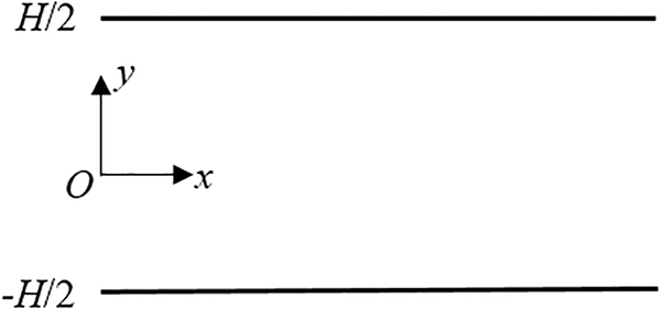
Schematics of Poiseuille flow.

n = 1

The rheological equation is directly simplified into the following form: $μ = μ_{0}$ (12)

where the viscosity is a constant quantity that is independent of the shear rate. Regarding the Newtonian Poiseuille flow, the theoretical solution is derived as follows: $u (y) = \frac{1}{2} (- \frac{1}{μ_{0}} \frac{\partial p}{\partial x}) [{(\frac{H}{2})}^{2} - {|y|}^{2}]$ (13)

where ∂p/∂x is the pressure gradient in the x-direction, and H is the distance between two parallel plates. The maximum velocity occurs at the middle position where y = 0: $u_{max} = u (0) = \frac{1}{2} (- \frac{1}{μ_{0}} \frac{\partial p}{\partial x}) {(\frac{H}{2})}^{2}$ (14)

In the numerical simulation, both the distance between two parallel plates H and the length of the plates L are set as 1. ∂p/∂x is −3 × 10⁻³, μ₀ is 0.02 and the lattice nodes are 200 × 200. The comparison is shown in Figure 3. The numerical solution is well consistent with the theoretical solution.

FIG. 3.

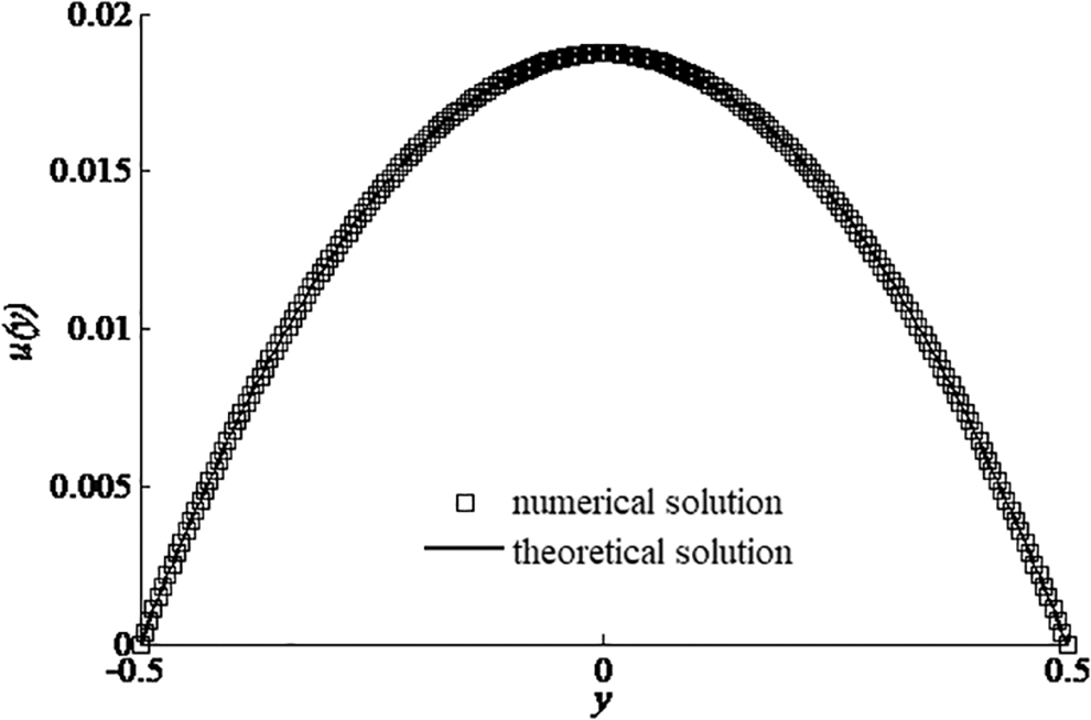
Comparison of numerical and theoretical solutions for n = 1.

n = 0.3568

When n = 0.3568, the rheological behavior is almost the same as that of the power-law fluid at n = 0.708.³² The values of the other parameters remain unchanged. Regarding power-law fluids, the theoretical solution of Poiseuille flow is: $u (y) = \frac{n}{n + 1} {(- \frac{1}{μ_{0}} \frac{\partial p}{\partial x})}^{\frac{1}{n}} [{(\frac{H}{2})}^{\frac{n + 1}{n}} - {|y|}^{\frac{n + 1}{n}}]$ (15)

whose maximum velocity is expressed as follows: $u_{max} = u (0) = \frac{n}{n + 1} {(- \frac{1}{μ_{0}} \frac{\partial p}{\partial x})}^{\frac{1}{n}} {(\frac{H}{2})}^{\frac{n + 1}{n}}$ (16)

The results in Figure 4 imply that the numerical solution of n = 0.3568 agrees with the theoretical solution of n = 0.708, which further demonstrates the effectiveness and accuracy of the proposed method.

FIG. 4.

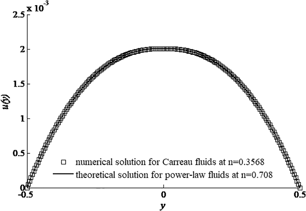
Comparison of Carreau fluids of n = 0.3568 and power-law fluids of n = 0.708.

Effects of Multiple Linear Obstacles on the Flow of Ceramic Slurry

Basic conditions

The rectangular channel shown in Figure 5b is obtained by fully expanding the screw channel in Figure 5a. As mentioned in the Introduction, the viscous slurry generates obstacles on the wall, which is shown in Figure 5b. The existing obstacles may have effects on the flow and further affect the following printing process. Thus, it is necessary to investigate the fluid flow carefully. The basic conditions of the flow channel are set as follows. The height and length of the channel are 4 and 8 cm, respectively. The lattice numbers are correspondingly set as 200 × 400 for MRT LBM simulation. The inlet velocity is described as a parabola, which accords with the actual situation. The maximum and minimum values are 0.8 and 0 m/s, respectively.

FIG. 5.

Single screw extruder. (a) Structure of the extruder. (b) Expansion of the extruder.

The geometry of an obstacle is always irregular; therefore; it is difficult to conduct accurate numerical simulations according to the actual situation. In essence, an irregular geometry is always composed of lines and/or arcs. Thus, analyzing the cases with linear or arcuate geometrical elements can contribute to understanding the universal mechanism. In the current work, the obstacle with interactive elements is analyzed. As shown in Figure 6, three situations are considered in detail. The line–line interactive situation is shown in the first figure, the considered factors include the positions, vertical sizes, and angles. In the second figure, the line–arc interactive situation is given. The influencing factors are the position, the angle between the line and tangent, and the first generated element (arc or line). The arc–arc interactive situations are shown in the third figure. The considered factors include the positions, vertical sizes, and the centers of the arcs (inside or outside the obstacle). The mentioned positions are common factors in three situations, which refers to the horizontal distance between the obstacle and the outlet.

FIG. 6.

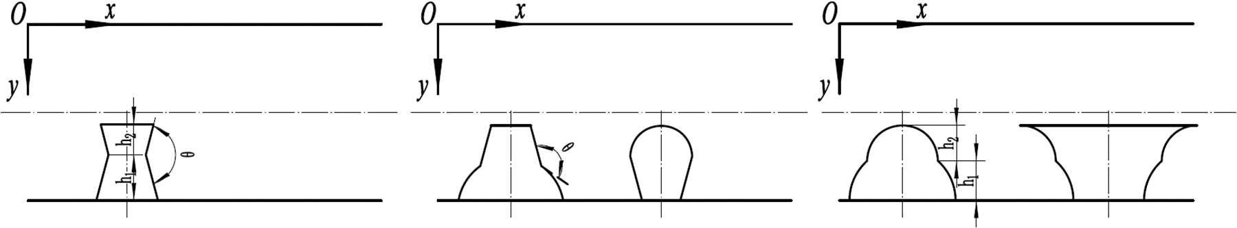
Different situations of the obstacles.

Line–line interactive cases

In this part, the line–line interactive cases are investigated. The main factors to consider are the angles, vertical sizes, and positions. Figure 7a, taking it as an example, gives the specific information of cases 1–3, where θ is the angle, h₁ and h₂ are the vertical sizes, and the different colors express different x-positions. Three cases have the same angles and vertical sizes, and the only difference is in the x-position. The streamline figures are given in Figure 7b–d. The yellow color represents the high-velocity zone, whereas the blue color corresponds to the low-velocity zone. The top-left corner of the obstacle causes a sudden change of flow. The obstacle forces the high-velocity zone to move up. The considerable vortex occurs at the back of the obstacle. The left edge of the vortex is dependent on the geometry of the right edge of the obstacle.

FIG. 7.

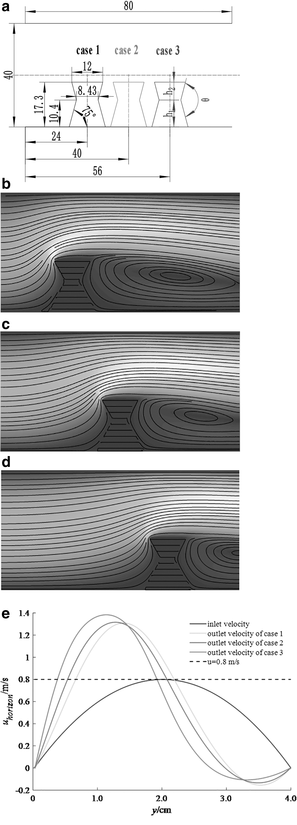
Simulation results of cases 1–3. (a) Specific situations of cases 1–3. (b) Streamlines of case 1. (c) Streamlines of case 2. (d) Streamlines of case 3. (e) Outlet velocity distributions of cases 1–3.

The horizontal dimension of the back vortex is large; therefore, when the obstacle is closer to the outlet, the vortex is unfinished. The outlet velocity distribution of each case is given in Figure 7e. The maximum outlet velocity of each case has been increased greatly when compared with that of the inlet velocity. The center of the high-velocity zone is determined by the position of the obstacle. Figure 7e implies that when the obstacle is much closer to the outlet, the higher position of the center is presented. Owing to the back vortex is not finished in each case, a different extent of negative velocity appears.

When the angle θ is larger than π, three cases are discussed. The specific situations of the cases are shown in Figure 8a. The streamlines shown in Figure 8b–d are relatively different from that of cases 1–3. First, a small vortex and turbulence tend to form at the front and back corners of the obstacle, respectively. Then, the left edge of the back vortex deforms because of the geometry of the right edge of the obstacle. The top-left corner of the obstacle is still the sudden change point of the flow direction. The distance between the obstacle with the outlet determines whether the back vortex can be fully developed. The outlet velocity distributions are shown in Figure 8e. The results are similar to that of cases 1–3. Thus, the main difference in cases 1–3 with cases 4–6 is embodied in the flow process.

FIG. 8.

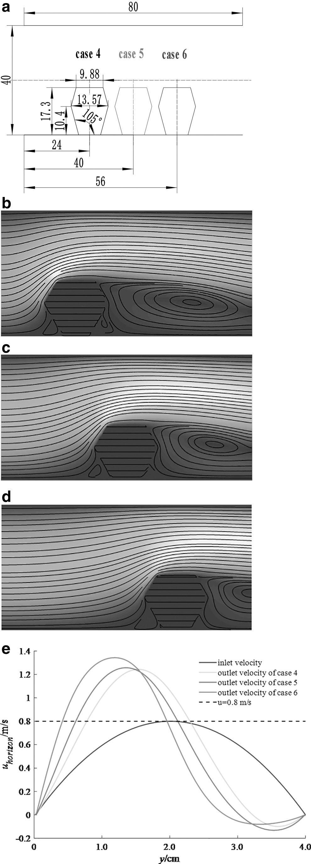
Simulation results of cases 4–6. (a) Specific situations of cases 4–6. (b) Streamlines of case 4. (c) Streamlines of case 5. (d) Streamlines of case 6. (e) Outlet velocity distributions of cases 4–6.

As shown in Figure 9, when compared with cases 1–3, the main difference of the situation is that the vertical size h₁ is less than h₂. The streamlines are similar to cases 1–3. Owing to the difference in the vertical size, the left part of the back vortex tends to locate at a lower position compared with cases 1–3. The outlet velocity distributions of the three cases shown in Figure 9e are analogous to that of cases 1–3.

FIG. 9.

Simulation results of cases 7–9. (a) Specific situations of cases 7–9. (b) Streamlines of case 7. (c) Streamlines of case 8. (d) Streamlines of case 9. (e) Outlet velocity distributions of cases 7–9.

In Figure 10, the angle θ is larger than π. The lower-left vortex tends to flow into the back corner of the obstacle. The phenomenon is not obvious when compared with cases 4–6. No apparent vortex or turbulence appears at the back corner. It is noted that the horizontal size of the back vortex changes with the position of the obstacle. When the obstacle is closer to the outlet, the horizontal size is smaller. The other results, including the outlet velocity distributions, are similar to that of cases 4–6.

FIG. 10.

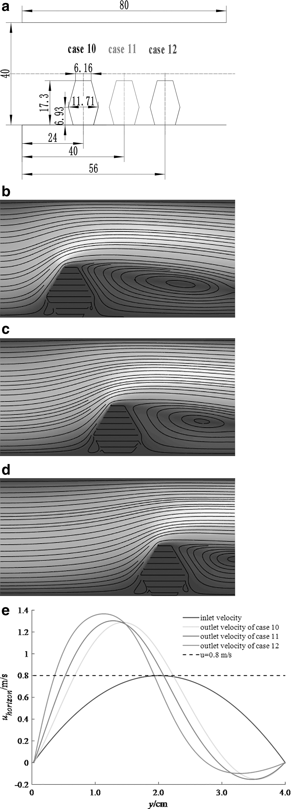
Simulation results of cases 10–12. (a) Specific situations of cases 10–12. (b) Streamlines of case 10. (c) Streamlines of case 11. (d) Streamlines of case 12. (e) Outlet velocity distributions of cases 10–12.

In Table 2, the specific simulation results of cases 1–12, including maximum and minimum velocity, corresponding Y-coordinates, and the coordinate values of vortex core are listed. When referring to the factor of vertical sizes, the vertical size h₁ is larger than h₂ in cases 1–6, while h₁ is less than h₂ in cases 7–12. The results show that the minimum velocities of cases 1–3 are smaller compared with cases 7–9. Cases 10–12 present higher maximum velocities and smaller minimum velocities when compared with cases 4–6. In addition, the centers of maximum and minimum velocities in cases 10–12 are located at the lower position, and the vortices cores are closer to the bottom wall.

Table 2.

Simulation Results of Cases 1–12

No.	Maximum velocity (m/s)	Y-coordinate of the maximum velocity (cm)	Minimum velocity (m/s)	Y-coordinate of the minimum velocity (cm)	Coordinate values of vortex core (cm)
Case 1	1.3087	1.40	−0.1542	3.53	(5.88, 2.79)
Case 2	1.3163	1.28	−0.1333	3.50	(6.67, 2.83)
Case 3	1.3835	1.14	−0.1066	3.31	(7.92, 2.75)
Case 4	1.2436	1.54	−0.0988	3.60	(5.63, 2.92)
Case 5	1.2576	1.36	−0.1314	3.54	(6.75, 2.83)
Case 6	1.3437	1.18	−0.0803	3.32	(7.96. 2.79)
Case 7	1.2986	1.42	−0.1488	3.54	(5.75, 2.79)
Case 8	1.3184	1.28	−0.1039	3.51	(6.63, 2.83)
Case 9	1.3795	1.16	−0.0946	3.32	(7.96, 2.75)
Case 10	1.2884	1.44	−0.1511	3.55	(5.63, 2.83)
Case 11	1.3034	1.28	−0.1537	3.47	(6.79, 2.75)
Case 12	1.3669	1.14	−0.0984	3.28	(7.92, 2.67)

Regarding the factor of angles, θ in cases 1–3 and 7–9 are smaller compared with cases 4–6 and 10–12. In cases 1–3, the maximum velocities are higher and the minimum velocities are smaller when compared with cases 4–6. The corresponding extreme points of the velocities and vortices cores are closer to the bottom wall in cases 4–6. Cases 7–9 show higher maximum velocities, whereas cases 10–12 present smaller minimum velocities.

Line–arc interactive cases

The second considered situation is line–arc interaction. The main influencing factors include the angles γ, positions, situations of the arcs (the arc is below or above the linear elements).

In Figure 11, the specific situations are as follows: the angle between the line and the arc is large, the arc is below the line, and the center of the arc is inside of the obstacle. Three different positions of the obstacle are investigated further. As shown in Figure 11b–d, the high-velocity zone is forced by the obstacle to move up, and the flow has a sudden change at the top-left corner. In case 13, the back vortex is almost finished, whereas only half of the vortex is done in case 15. The unfinished vortex leads to a negative velocity. With the obstacle approaching the outlet, the vortex core gradually moves to the geometrical center of the vortex. The outlet velocities’ distributions in further validate the above conclusion.

FIG. 11.

Simulation results of cases 13–15. (a) Specific situations of cases 13–15. (b) Streamlines of case 13. (c) Streamlines of case 14. (d) Streamlines of case 15. (e) Outlet velocity distributions of cases 13–15.

In Figure 12, the mentioned angle is smaller compared with Figure 11. When compared with the above three cases, the main difference is in the geometry of the left edge of the back vortex, which is dependent on the geometry of the right edge of the obstacle. In addition, there are differences in the size and position of the vortex core. The velocities’ distributions of cases 16–18 are shown in Figure 12e, which is similar to cases 13–15.

FIG. 12.

Simulation results of cases 16–18. (a) Specific situations of cases 16–18. (b) Streamlines of case 16. (c) Streamlines of case 17. (d) Streamlines of case 18. (e) Outlet velocity distributions of cases 16–18.

When the arcuate elements are above the linear elements, the first three investigated cases are shown in Figure 13a, where the angle between the line and the tangent line is relatively large. In Figure 13b–d, they imply that the horizontal size of the back vortex decreases when the obstacle is close to the outlet, the horizontality gets better, meanwhile, the size of the vortex core also changes. In addition, the slurry flows across the surface of the obstacle smoothly without obvious sudden-changed points. In Figure 13e, the highest maximum velocity occurs in case 21, whereas the magnitudes of the maximum velocities in cases 19–20 are almost the same.

FIG. 13.

Simulation results of cases 19–21. (a) Specific situations of cases 19–21. (b) Streamlines of case 19. (c) Streamlines of case 20. (d) Streamlines of case 21. (e) Outlet velocity distributions of cases 19–21.

When the angle changes, three cases are investigated as follows. In the front and back of the obstacle, turbulence occurs at the corner when the obstacle is far away from the outlet. If the obstacle is close to the outlet, the lower-left vortex tends to flow into the back corner of the obstacle. Similar velocity distributions are given in Figure 14e. When the obstacle is closer to the outlet, the center of the high-velocity zone is higher, and the maximum outlet velocity is the highest of the three cases.

FIG. 14.

Simulation results of cases 22–24. (a) Specific situations of cases 22–24. (b) Streamlines of case 22. (c) Streamlines of case 23. (d) Streamlines of case 24. (e) Outlet velocity distributions of cases 22–24.

In Table 3, the specific simulation results are listed. The arcuate elements are located at the bottom in cases 13–18, whereas the linear elements are located at the bottom in cases 19–24. The larger maximum velocities and smaller minimum velocities are presented in cases 13–18 compared with cases 19–24. In addition, Y-coordinates of vortices cores are located at lower positions. The angles in cases 13–15 are larger than those in cases 16–18. The results show that the vortices cores in cases 13–15 are located at the right positions when compared with those in cases 16–18. The angles in cases 19–21 are smaller than those in cases 22–24. The vortices cores in cases 19–21 are lower compared with cases 22–24. In summary, the angle only has a little effect on the flow.

Table 3.

Simulation Results of Cases 13–24

No.	Maximum velocity (m/s)	Y-coordinate of the maximum velocity (cm)	Minimum velocity (m/s)	Y-coordinate of the minimum velocity (cm)	Coordinate values of vortex core (cm)
Case 13	1.2689	1.48	−0.1119	3.60	(6.29, 2.97)
Case 14	1.2687	1.32	−0.1390	3.50	(6.94, 2.88)
Case 15	1.3359	1.16	−0.0984	3.31	(7.94, 2.79)
Case 16	1.2506	1.52	−0.1243	3.56	(6.00, 2.88)
Case 17	1.2703	1.36	−0.1311	3.55	(6.79, 2.85)
Case 18	1.3532	1.18	−0.0755	3.33	(7.91. 2.82)
Case 19	1.2184	1.56	−0.0809	3.65	(5.76, 2.92)
Case 20	1.2345	1.36	−0.1263	3.52	(6.75, 2.83)
Case 21	1.2982	1.20	−0.0957	3.34	(7.96, 2.71)
Case 22	1.2008	1.56	−0.0847	3.65	(4.96, 2.54)
Case 23	1.2328	1.36	−0.1241	3.53	(6.75, 2.79)
Case 24	1.2993	1.20	−0.0983	3.35	(7.96, 2.33)

Arc–arc interactive cases

In this section, the arc–arc interactive cases are analyzed (Figure 15, Table 4). The main considered influencing factors include the positions, vertical sizes (h₁ and h₂), and the center of the arc is inside or outside the obstacle. In cases 25–27, the vertical size h₁ is larger than h₂, and the center of the arc is inside the obstacle, whereas the positions of the three cases are different. The left edge of the back vortex is determined by the right edge of the obstacle. The position of the obstacle has an important effect on the length of the high-velocity zone. When the obstacle is much closer to the outlet, the horizontal size of the back vortex decreases, and the center of the high-velocity zone becomes higher. In addition, it shows that the streamlines are slightly confused in case 26. The velocity distributions in Figure 15e validate the above conclusions. The negative velocity occurs in each case. Although the back vortex in case 27 is the most severely unfinished, the negative velocity presented is the smallest.

FIG. 15.

Simulation results of cases 25–27. (a) Specific situations of cases 25–27. (b) Streamlines of case 25. (c) Streamlines of case 26. (d) Streamlines of case 27. (e) Outlet velocity distributions of cases 25–27.

Table 4.

Simulation Results of Cases 25–36

No.	Maximum velocity (m/s)	Y-coordinate of the maximum velocity (cm)	Minimum velocity (m/s)	Y-coordinate of the minimum velocity (cm)	Coordinate values of vortex core (cm)
Case 25	1.1881	1.60	−0.1404	3.64	(4.25, 2.67)
Case 26	1.2276	1.37	−0.1177	3.54	(6.83, 2.83)
Case 27	1.3021	1.20	−0.0629	3.20	(7.96, 2.67)
Case 28	1.4017	1.42	−0.1465	3.50	(7.04, 2.75)
Case 29	1.3820	1.28	−0.1036	3.46	(7.29, 2.46)
Case 30	1.4052	1.18	−0.0716	3.29	(7.96. 2.63)
Case 31	1.2251	1.64	−0.0825	3.68	(6.15, 3.03)
Case 32	1.2233	1.38	−0.1221	3.54	(6.85, 2.94)
Case 33	1.3023	1.20	−0.0665	3.27	(7.94, 2.79)
Case 34	1.3958	1.40	−0.1480	3.48	(7.35, 2.91)
Case 35	1.3851	1.28	−0.1124	3.46	(7.47, 2.88)
Case 36	1.4053	1.19	−0.0713	3.30	(7.97, 2.79)

When compared with cases 25–27, the centers of the arcs in cases 28–30 are outside the obstacles. In case 28, the turbulence appears in the left corner, a flat vortex occurs above the obstacle, and the top-left corner is the sudden-changed point of the flow. With the obstacle approaching the outlet, the mentioned flat vortex disappears, and the turbulence changes into a small vortex gradually. The positions also have effects on the sizes of the vortices cores. It is noted that the turbulence also appears in the right corner of case 29. In Figure 16e, the velocity distributions imply that the difference in the magnitudes of the maximum outlet velocities is quite small, which is different from other cases. The obstacle in case 30 is closest to the outlet, therefore the center of the high-velocity zone is the highest.

FIG. 16.

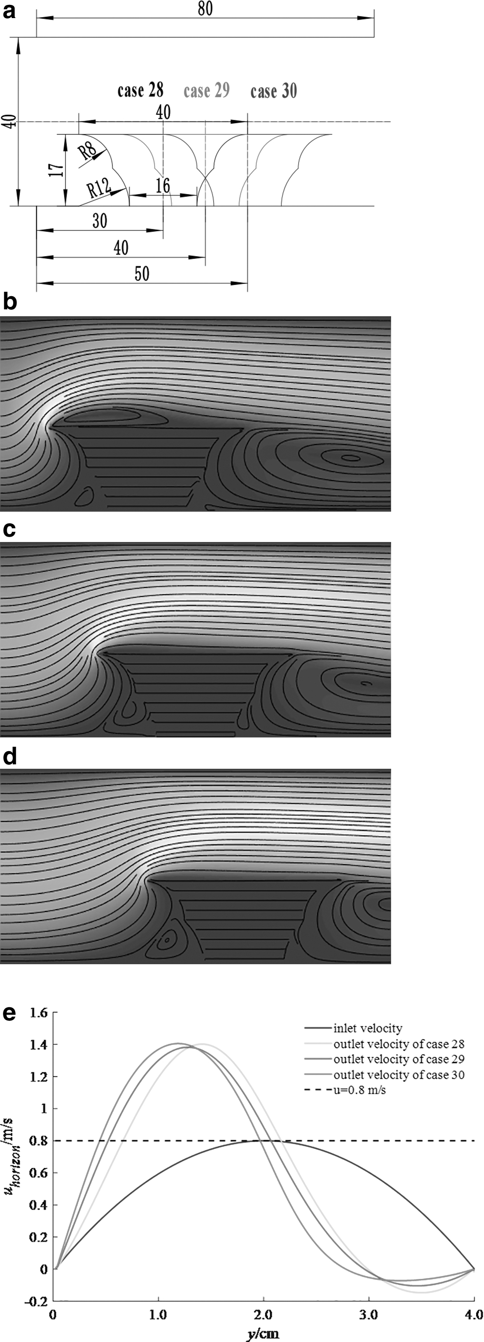
Simulation results of cases 28–30. (a) Specific situations of cases 28–30. (b) Streamlines of case 28. (c) Streamlines of case 29. (d) Streamlines of case 30. (e) Outlet velocity distributions of cases 28–30.

When compared with cases 25–27, the vertical size h₁ is smaller than h₂ in cases 31–33. The morphologies and the centers of the back vortices severely differ from that of cases 25–27. The vortex core in case 31 is located to the right, whereas that in case 24 is located to the left. Owing to the larger vertical size h₂, the lower-left vortex tends to flow into the right corner of the obstacle. The turbulence occurs gradually with the obstacle approaching the outlet. The velocity distributions in Figure 17e show that the maximum velocities of the cases do not obey the rule mentioned above, where the maximum velocity of case 32 is the smallest in three cases.

FIG. 17.

Simulation results of cases 31–33. (a) Specific situations of cases 31–33. (b) Streamlines of case 31. (c) Streamlines of case 32. (d) Streamlines of case 33. (e) Outlet velocity distributions of cases 31–33.

In cases 34–36 (Fig. 18a), the vertical size h₂ is much larger than h₁, and the center of the arc is outside the obstacle. The flow near the top surface of the obstacle is unstable. In particular, the flat vortex appears above the top surface. The turbulence formed in the front corner of the obstacle changes into a small vortex gradually with the obstacle approaching the outlet. It is not obvious when compared with cases 28–30. As shown in Figure 18e, the maximum velocity of case 35 is the smallest of three cases. The phenomenon is similar to that of cases 31–33. In addition, the centers of the maximum velocities in cases 35–36 are close.

FIG. 18.

Simulation results of cases 34–36. (a) Specific situations of cases 33–36. (b) Streamlines of case 33. (c) Streamlines of case 35. (d) Streamlines of case 36. (e) Outlet velocity distributions of cases 34–36.

As shown in the first figures in Figures 15–18, the situations of cases 25–36 are set as follows. The vertical sizes h₁ are larger than h₂ in cases 25–30, then the centers of the arcs in cases 25–27 are inside the obstacles while the centers in cases 28–30 are outside. In cases 31–36, the vertical sizes h₁ are smaller than h₂, then the centers of the arcs in cases 31–33 are inside, whereas that in cases 33–36 are outside. When we compare cases 25–27 with cases 28–30, the positions of the maximum velocities are lower, the maximum velocities are higher, and the vortices cores are located at the right side, whereas the minimum velocities are similar. Similar results to the above cases are obtained in cases 31–36. When cases 31–33 are compared with cases 25–27, all centers of the arcs are inside the obstacles, and the vortices cores are at lower locations. There are no obvious differences in the other parameters. When we compare cases 28–30 with cases 34–36, all the centers of the arcs are outside the obstacles, and the vortices cores are located at higher positions. Similar results are presented when cases 28–30 are compared with cases 34–36.

Discussion

The discussed obstacles are always irregular, whereas the irregular geometries are composed of linear, arcuate, and interactive elements. Thus, the regular geometrical elements are used to reveal the general effect mechanism of the obstacles. In the present work, the interactive elements, including line–line, line–arc, and arc–arc situations are investigated in detail. To efficiently conduct the numerical simulations, a modified MRT LBM based on a pseudo external force is proposed, which can improve the stability and accuracy of the non-Newtonian SiC slurry.

In three different situations, the common considered influencing factor is the position. According to the figures and the data given in the tables, they show that the positions of the obstacles have important effects on the flow. With approaching the outlet, the maximum velocities become larger, the points of the maximum and minimum velocities move up gradually, and the vortices cores tend to move toward the right and up. It is noted that the minimum velocities are always negative because of the unfinished back vortex. The minimum velocity increases gradually when the obstacle is closer to the outlet in line–line and arc–arc interactive cases, whereas the minimum velocity appears in the situation whose obstacle is located at the middle position when two different elements are considered in one obstacle.

Except for the positions, different factors are considered in different situations. In line–line interactive cases, the angle and vertical size are the other two considered factors. The results show that when the angle θ is larger than π, the case with a smaller vertical size h₁ presents a larger maximum velocity and a smaller minimum velocity. The vortex core and Y-coordinates of the maximum and minimum velocity are located at a higher position. However, when the angle θ is less than π, the vertical size almost has no effect on the outlet velocity and the vortex core. In addition, the streamlines imply that sudden changes in the flow direction and velocity occur when the flow encounters the top-left point of the obstacle. A small vortex or turbulence appears at the front and back corner in cases whose angles are larger than π.

In line–arc interactive cases, another two considered factors are the angle and the position of the element, for example, in cases 13–18, the arcuate elements are first generated on the wall, whereas the linear elements are generated in cases 19–24. The former six cases show larger maximum velocities and smaller minimum velocities when compared with the latter six cases. In addition, the corresponding points of the maximum and minimum velocities are located at lower positions in cases 19–24. When the factor of angles is considered, it can be found that only the coordinates of the vortices cores change slightly, which implies that the angles have the smallest influence on the flow. It is noted that there are no sudden changes in cases 19–24 whose arcuate elements are located above the linear elements.

In arc–arc interactive cases, the considered factors include the vertical sizes and the positions of the geometrical centers of the arcs (the centers are inside or outside the obstacles). The simulation results imply that when the geometrical centers of the arcs are outside the obstacles, the larger maximum outlet velocities can be obtained, and the points of the maximum velocities are higher. If the vertical size h₁ is smaller than h₂ in a case, the vortex core tends to be closer to the bottom wall.

Conclusion

In the present work, the effects of the interactive elements are investigated to understand the specific flow of the non-Newtonian SiC slurry in DIW technology. Three different situations are listed to explain the interaction. Different influencing factors for different situations are considered to have effects on the flow. Once the obstacle occurs, the maximum velocity increases more than 50% when compared with inlet velocities.

The positions are the common and important factors, which mainly affect the streamlines and outlet velocities. When the obstacle is closer to the outlet, the outlet velocity increases gradually, the back vortex tends to be unfinished, and the position of the vortex core changes. In line–line interactive situations, the angles have effects on the streamlines and maximum outlet velocities. In particular, the geometry of the left edge of the back vortex is determined by the right edge of the obstacle. When the angle is larger than π, turbulence even in a small vortex may occur in the corners. In line–arc interactive situations, when the arcuate elements are below the linear elements, the corresponding cases present larger maximum velocities, and the points of the maximum velocities are higher. The angles mainly affect the geometries of the streamlines. In the arc–arc interactive situations, the cases whose centers of the arcs are outside the obstacles show larger maximum outlet velocities and higher points of the maximum velocities. The vertical sizes also mainly affect the streamlines.

In the experiments, the outlet velocities are always calculated by use of the empirical formulas, whereas the possible obstacles are ignored. To understand the actual situations, the flow with an obstacle(s) should be considered seriously. According to the simulations, the obstacles increase the outlet velocities to some extent, and the flow directions change when compared with the inlet velocities. The results can provide references for the actual outlet velocity distributions, and contribute to practical optimization of the printing parameters.

Footnotes

Author Disclosure Statement

No competing financial interests exist.

Funding Information

This work is supported by the National Natural Science Foundation of China (Grant No. 32072785), Natural Science Foundation of the Jiangsu Higher Education Institutions of China (Grant No. 20KJB470008), and China Postdoctoral Science Foundation (No. 2020M671617).

References

, Liu

, Liao

, et al. Ultra-high temperature ceramics melting temperature prediction via machine learning. Ceram Int, 2019; 45:18551–18555.

Zheng

, Wang

, Gao

, et al. Design of high-reflectance ceramic materials based on the first-principle calculation. J Mater Sci, 2020; 55:5481–5487.

Ovsyannikov

, Popov

, Perfilov

, et al. High-hardness ceramics based on boron carbide fullerite derivatives. Phys Solid State, 2017; 59:327–330.

Neuman

, Brown-Shaklee

, Hilmas

, et al. Titanium diboride-silicon carbide-boron carbide ceramics with super-high hardness and strength. J Am Ceram Soc, 2018; 101:497–501.

, Zhang

, Huang

, et al. Effect of extrusion on viscoelastic slurry 3D print quality: numerical analysis and experiment validation. SN Appl Sci, 2019; 1:1036.

, Liu

, Zhang

, et al. 3D printed ceramic phosphor and the photoluminescence property under blue laser excitation. J Eur Ceram Soc, 2019; 39:2731–2738.

Yang

, Zeng

, Zhang

. 3D printing of alumina ceramic parts by heat-induced solidification with carrageenan. Mater Lett, 2019; 255:126564.

Ding

, He

, Zhang

, et al. Stereolithography 3D printing of SiC ceramic with potential for lightweight optical mirror. Ceram Int, 2020; 46:18785–18790.

Zhang

, Carloni

, Wu

. 3D printing of transparent YAG ceramics using copolymer-assisted slurry. Ceram Int, 2020; 46:17130–17134.

10.

, Hwang

, Kim

, et al. Extrusion-based 3D direct ink writing of NiZn-ferrite structures with viscoelastic ceramic suspension. Ceram Int, 2020; 46:6469–6476.

11.

Tang

, Hao

, Li

, et al. Dual gradient direct ink writing for formation of kaolinite ceramic functionally graded materials. J Alloys Compd, 2019; 814:152275.

12.

Abdeljawad

, Bolintineanu

, Cook

, et al. Sintering processes in direct ink write additive manufacturing: a mesoscopic modeling approach. Acta Mater, 2019; 169:60–75.

13.

Revelo

, Colorado

. 3 D printing of kaolinite clay ceramics using the Direct Ink

Writing

(DIW) technique. Ceram Int 2018, 44:5673–5682.

14.

Jones

, Seeley

, Cherepy

, et al. Direct ink write fabrication of transparent ceramic gain media. Opt Mater, 2018; 75:19–25.

15.

Liu

, Liu

. An immersed transitional interface finite element method for fluid interacting with rigid/deformable solid. Eng Appl Comput Fluid Mech, 2019; 13:337–358.

16.

Fang

, Li

. Fully discrete finite element methods for two-dimensional bingham flows. Math Probl Eng, 2018; 2018:4865849.

17.

Martins

, Vaz

, Zdanski

. A note on a derivative scheme for the finite volume method applied to incompressible viscous fluid. Contin Mech Thermodyn, 2018; 30:943–952.

18.

Suliman

, Oxtoby

, Malan

, et al. A matrix free, partitioned solution of fluid-structure interaction problems using finite volume and finite element methods. Eur J Mech B Fluids, 2015; 49:272–286.

19.

Pantokratoras

. Steady flow of a power-law non-Newtonian fluid across an unconfined square cylinder. J Appl Mech Tech Phys, 2016; 57:264–274.

20.

Husain

, Siddiqui

, Khan

. Effect of geometrical parameters on natural convection of water in a narrow annulus. Prog Nucl Energy, 2018; 112:146–161.

21.

Zhou

, Bayazitoglu

. Developing laminar natural convection of power law fluids in vertical open ended channel. Int J Heat Mass Transf, 2019; 128:354–362.

22.

Kumar

, Dhiman

, Baranyi

. CFD analysis of power-law fluid flow and heat transfer around a confined semi-circular cylinder. Int J Heat Mass Transf, 2015; 82:159–169.

23.

Kefayati

, Huilgol

. Lattice Boltzmann method for the simulation of the steady flow of a Bingham fluid in a pipe of square cross-section. Eur J Mech, 2017; 65:412–422.

24.

Zhang

, Chen

, Sun

, et al. Free-surface simulations of Newtonian and non-Newtonian fluids with the lattice Boltzmann method. Acta Geol Sin Engl Ed, 2016; 90:999–1010.

25.

Khabazi

, Taghavi

, Sadeghy

. Peristaltic flow of Bingham fluids at large Reynolds numbers: a numerical study. J Nonnewton Fluid Mech, 2016; 227:30–44.

26.

, Sun

, Wang

, et al. A universal modified MRT LBM for common non-Newtonian fluids and their applications. Mech Mater, 2019; 139:103187.

27.

Qiu

, Yu

. 3D simulation of self-compacting concrete flow based on MRT-LBM. Adv Mater Sci Eng, 2018; 2018:5436020.

28.

Yang

, Wang

. Multiple-relaxation-time lattice Boltzmann study of the magnetic field effects on natural convection of non-Newtonian fluids. Int J Mod Phys C, 2017; 28:1750138.

29.

Molla

, Nag

, Thohura

, et al. A graphics process unit-based multiple-relaxation-time lattice Boltzmann simulation of non-Newtonian fluid flows in a backward facing step. Computation, 2020; 8:83.

30.

Sajjadi

, Delouei

, Izadi

, et al. Investigation of MHD natural convection in a porous media by double MRT lattice Boltzmann method utilizing MWCNT-Fe3O4/water hybrid nanofluid. Int J Heat Mass Transf, 2019; 132:1087–1104.

31.

Guo

, Zheng

, Shi

. Discrete lattice effects on the forcing term in the lattice Boltzmann method. Phys Rev E, 2002; 65:046308.

32.

Shibeshi

, Collins

. The rheology of blood flow in a branched arterial system. Appl Rheol, 2005; 15:398–405.