Correlating Laser Additive Manufacturing Process with Heat Source Coefficients by Integrated Experimental and Numerical Models

Abstract

Numerical modeling of additive manufacturing processes is often conducted to predict both thermal and mechanical effects such as distortions, residual stresses, and phase distributions. The prediction accuracy is highly dependent on an accurate representation of thermal field, especially heat sources. In this study, response surface methodology (RSM) is serially utilized and mutually mapped to understand the relationships between process parameters and heat source coefficients. First, the effects of process factors and heat source model coefficients on experimental and numerical bead geometry are, respectively, identified through analysis of variance on central composite designs. With influences mathematically quantified, heat source coefficients in accordance with experimental conditions are inversely solved using nonlinear least square method, followed by correlation with process factors. The results show that both the effects of process parameters and heat source coefficients on bead geometry characteristics can be modeled using quadratic polynomials. The connections between heat source coefficients and process variables can also be modeled using quadratic or lower polynomial functions with good accuracy. It is proven that the proposed RSM mapping method is feasible for heat process correlation. The research outcome provides a convenient and reliable method of heat source calibration for laser additive manufacturing.

Introduction

Laser additive manufacturing is a versatile prototyping process utilizing energy intensive laser beam as heat source to rapidly melt additive material (powder or wire) and obtain designated part geometry.¹ Owing to the advantageous features of high laser energy density, noncontact with workpiece, little postprocessing, and high productivity, laser additive manufacturing has been widely implemented for equipment production such as automotive, ship, aircraft, and astronautic vehicle.²

Understanding thermal gradient that workpiece experienced plays an important role in the process control of laser additive manufacturing. This is due to the fact that mechanical properties of laser additive manufactured components/parts are macroscopic outcomes of microscopic reactions and interactions that involved metal experiences during the cyclic heating and cooling process, including chemical-metallurgical reactions, grain growth, and phase transformation. All these reactions are controlled by thermal gradient of melt pool and the entire workpiece.³

However, it is of great difficulty to quantify temperature field of workpiece and local thermal gradients. In situ measurement of temperature is limited to certain points and external surfaces due to the characteristics of temperature sensors such as thermocouple and thermal infrared camera. Finite element method provides an efficient tool to compute the thermal field and thereafter residual stresses on the condition that relevant models are well calibrated.^4,5 As heat input models have been rendered to incorporate most physics of additive manufacturing process, it is of great significance to accurately define the parameters associated with the mathematical description of heat source so that numerical simulations yield reliable results close to experimental data.⁶

The methods proposed in literature for heat source calibration may be classified into three categories according to solution of temperature field: analytical, numerical, and semianalytical method. Analytical approach directly solves the partial differential equations of heat transfer describing laser additive manufacturing process to obtain temperature field of workpiece for calibration. Hitherto, numerous solutions have been proposed to obtain quasi-steady-state and transient temperature fields caused by point, line, plane, and volumetric heat sources.

Rosenthal⁷ presented closed-form analytical solutions for temperature field at quasi-steady state subject to point, line, and plane heat sources. Figure 1 illustrates the temperature distributions due to different types of heat sources. These models are a mathematical trick to avoid dealing with the real energy distribution of a heat source. They only provide accurate temperature distributions at sufficiently far positions from the weld. Manca et al.⁸ obtained quasi-steady-state temperature distribution with a circular Gaussian heat source moving in a finite depth plate.

FIG. 1.

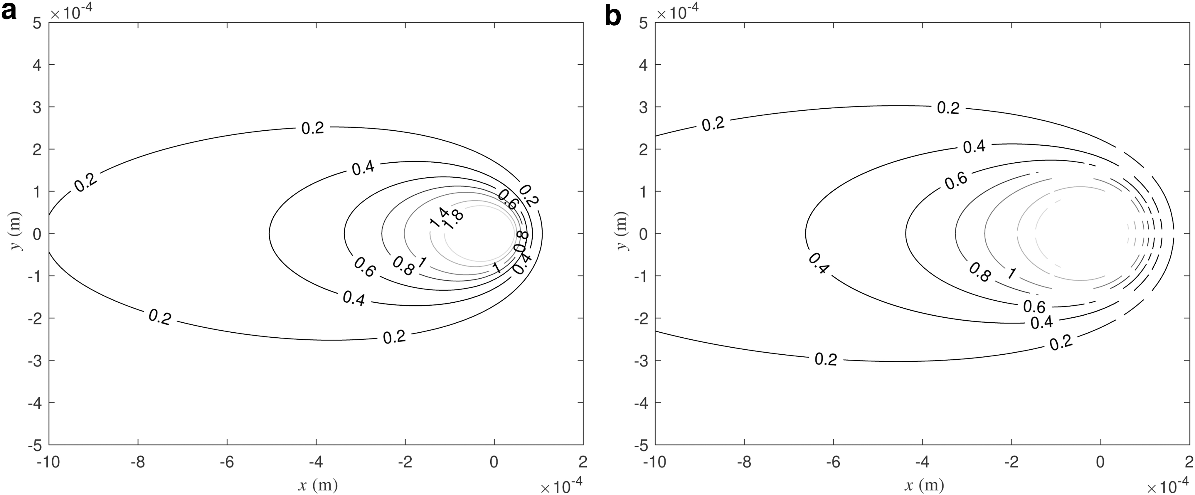
Temperature field for various heat sources. (a) Point heat source; (b) ellipsoidal heat source.

The solution is feasible when the radius of Gaussian spot is far smaller than the width and far greater than the plate thickness. Zubair and Chaudhry⁹ deduced solutions for transient temperature fields for a surface hardening infinite plate with finite thickness caused by a uniform rectangular heat source. The solution is still limited for constant properties and, therefore, is not applicable for situations where convective and radiation losses are important boundary conditions. Nguyen et al.¹⁰ obtained an analytical approximate model for a double ellipsoid heat source moving at a finite plate using Green's functions (GF).

The approximation was an effective analogy of energy input into the finite body from an infinite-body source. The limitation is that the solutions were effective for heat sources constantly moving in one of three Cartesian coordinates through an infinite domain. Araya and Gutierrez¹¹ developed an analytical transient solution for temperature field of a 3D finite plate with a Gaussian heat source in integral form using eigenfunction expansions.

To bridge various analytical heat transfer models, Myhr and Grong¹² established dimensionless maps to generally outline the quasi-steady-state temperature distribution pertaining to a moving heat source on different plates. Azar et al.¹³ implemented the solution for discretely distributed point heat source model to determine the geometrical parameters of Goldak's double-ellipsoidal model. The front and rear dimensions of the heat flux distribution were obtained based on the end crater geometry of weld track.

But the heat flux intensities of discrete ellipsoids were determined by matching the maximum temperature with experimental data. Wu et al.¹⁴ calibrated both the melt pool geometry and thermal field by applying two adjustment ratios to the analytical temperature distribution of a finite thick plate based on single ellipsoidal stationary heat source. To improve computation efficiency, Wu et al.¹⁵ then rebuilt the model to split temperature distribution into two terms: one as a function of an earlier temperature distribution, and the other as a function of the newly applied arc power.

Fu et al.¹⁶ utilized a neural network trained by the Levenberg–Marquardt algorithm to correlate the parameters of a double ellipsoid heat source model with analytical computed weld pool geometries. Compared with Goldak et al.'s¹⁷ results, the established neural network reduced the computation consumption to predict the parameters of heat source model. But a higher prediction error of 14.28% was obtained in the weld pool geometry. Ning et al.^18,19 developed a quasi-analytical solution to estimate the in-process temperature in powder feed metal additive manufacturing based on absolute coordinate.

Laser beam is predicted by a moving point heat source solution. Convection and radiation at the part boundary is symbolized by a heat sink. Thermal profiles are obtained by superimposing heat rise/loss due to the heat transfer boundary conditions, that is, laser power absorption, scanning strategy, and latent heat. The problems for closed-form analytical solutions are that thermophysical properties of materials were assumed to be temperature independent. What is worse, the studied domain for analytical solution is limited to simple forms such as plates, cylinders, and infinite geometry. Moreover, the analytical solutions may overestimate the temperature field, as mathematical infinity is reached at the location of point and line heat source.²⁰

Numerical method discretizes studied complex geometry into finite domains and transforms partial differential equations into an assembly of linear forms for solution. Kim et al.²¹ calibrated a modified Gaussian 3D heat source by the trial and error method to fit the numerically calculated shape and size of molten zone with experimental data for pulsed laser welding of AISI 304 stainless steel plate. The calibration procedure is simple; however, it is time-consuming to iteratively change parameters and check the result divergence.

It is worse that the calibration results are inherently inaccurate and provides little information for newly encountered process conditions. To overcome the problems, many academics have been devoted to developing automated calibration programmes using optimization algorithms. Belitzki et al.²² presented a solution procedure to automatically identify the geometrical parameters of a double ellipsoid heat source through optimization algorithms. During calibration, the welding process was assumed to be quasi-stationary and weld pool geometry kept unchanged.

Chen et al.⁶ also programmed an interaction between finite element and optimization algorithm package to automatically calibrate heat source models and quantified the effects of welding process variables. Another automated calibration method proposed by Walker and Bennett²⁰ considered the mesh size optimization before inverse solution of the heat source parameters. The numerical method can model domains of complex geometry and include nonlinearities such as temperature-dependent thermal conductivity, specific heat, boundary conditions, latent heats of phase transformation, and microstructure evolution.

One big problem facing the numerical method is the serious time-consuming computation cost. As the number of heat source coefficients increases, the solution burden is exponentially exacerbated unless much parallel computation strategy and inverse algorithm are effectively applied.

Semianalytical approach provides another option for heat source calibration by solving the thermal fields of laser additive manufacturing process. The method retains the assumption of temperature-independent thermophysical properties so that Green's function method (GFM) can be applied for better accuracy and faster computation. Then, numerical method is applied to resolve the time integral involved in the GF solution. Majumdar and Xia²³ modeled the laser heating operations by coupling GFM with Romberg's algorithm for time integration.

Kidawa-Kukla²⁴ applied the GFM in conjunction with a time-partition method to solve a heat conduction problem with laser-type moving heat source. Veldman et al.²⁵ proposed a GFM-based method for a 2D problem on an infinite domain with a thin section by using a Taylor series in time. Cole et al.²⁶ developed a semianalytical source (SAS) method to solve nonlinear coupled equations through GFM, which recasts the boundary value problem into an integral equation (with nonlinear terms treated as source terms) for a reaction-diffusion problem.

The GF computation can be performed beforehand and stored, which is a particular advantage of SAS for rapid applications such as control of industrial processes and inverse problems. Çetin et al.²⁷ implemented SAS method for a 3D transient heat conduction problem with a piecewise constant heat source. They found that the SAS method is particularly suited for parallel computing. Nonlinearities related with temperature are still exempt for possible analytical part solution. Another disadvantage for semianalytical method is the limited situations for obtaining GF. It is also criticized for the uncertain computation cost for long duration process.

As additive manufacturing technologies are inherently suitable for producing complex mechanical parts, the effects of deposited geometry on the evolving thermal profile would limit the implementation of analytical solutions in this field. Therefore, raising the efficiency of numerical method becomes a good alternative to facilitate heat source calibration. In this study, a novel method integrating response surface methodology (RSM) with multiobjective optimization is proposed to calibrate heat source models and correlate the coefficients with laser additive manufacturing process.

Based on RSM, limited experimental and numerical runs are designed to study the effects of process parameters and heat source coefficients on experimental and numerical bead geometry characteristics, respectively. Heat source coefficients corresponding to experimental process conditions are then inversely solved using nonlinear least square method. At last, the effects of process conditions on heat source coefficients are correlated and modeled. The proposed heat process correlation method have a number of advantages, such as convenient operation, suitability for various heat source models and good prediction accuracy.

Methods

Response surface methodology

RSM, proposed by Box and Wilson,²⁸ is a comprehensive experiment design method for efficient identification of correlations between influencing factors and one or more responses. In RSM, experimental runs of orthogonality, ratability, and uniformity are proposed at locally representative points to analyze the effects of independent factors on dependent responses, including main and interaction effects. With quantitative models approximated, optimal response(s) can be achieved with regard to the influencing factors.²⁹

Generally, the relationship between system response and design variables subjects to $Y = ỹ (x) + δ,$ (1)

where $ỹ (x)$ is the approximate function for the unknown correlation, x = [x₁, x₂, · · ·, x_n] is an n dimension design variable, δ is the total error inclusive of random error, modeling error, and systematic error, and so on.

In practice, selection of the model function is subject to empirical engineering knowledge and low-order polynomials such as linear and quadratic models are frequently applied.³⁰

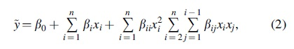
where β₀ is the minor error and β_i, β_ii, and β_ij are the polynomial coefficients for main effects, quadratic effects, and interaction effects, respectively. Owing to efficient correlating capacity, a novel method based on RSM is presented in the following section for heat process modeling.

Proposed method

To correlate heat source coefficients with influencing variables, serial RSM designs are required. The detail of proposed method for heat source modeling is illustrated as follows:

First, RSM design 1 is applied, for laser surfacing experiment, to correlate bead geometry characteristics (the number of responses should be no less than that of heat source coefficients. Here, the responses are width, depth, and area) with process parameters. The relationships may be denoted by f_i (P, v, and D_f), where P, v, and D_f are process parameters laser power, scanning speed, and defocusing distance, i = W, D, A represents the bead characteristics width, depth and area, respectively.

Second, RSM design 2 is implemented, for heat transfer finite element models, to investigate the influences of heat source parameters on the geometry characteristics of simulated bead. The correlations may be represented by g_i (η, r, c, and v), where η, r, and c are heat source coefficients absorption efficiency, heat radius, and height, respectively. The scanning speed v is considered as a variable here to bridge two design matrices.

Third, heat source parameters corresponding to experimental RSM 1 are identified through nonlinear least square method. With scanning speed known in RSM 1, the functions g_i (η, r, c, and v) are reduced into the form with three unknown coefficients, g_i (η, r, and c). The parameters are then evaluated by solving the problem: min

Lastly, the influences of laser surfacing parameters on the heat source model coefficients are investigated and mathematically correlated, as indicated by h_j (P, v, and D_f), where j indicates three coefficients η, r, and c.

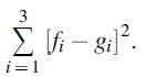
Figure 2 depicts the application sequence of heat process modeling method.

FIG. 2.

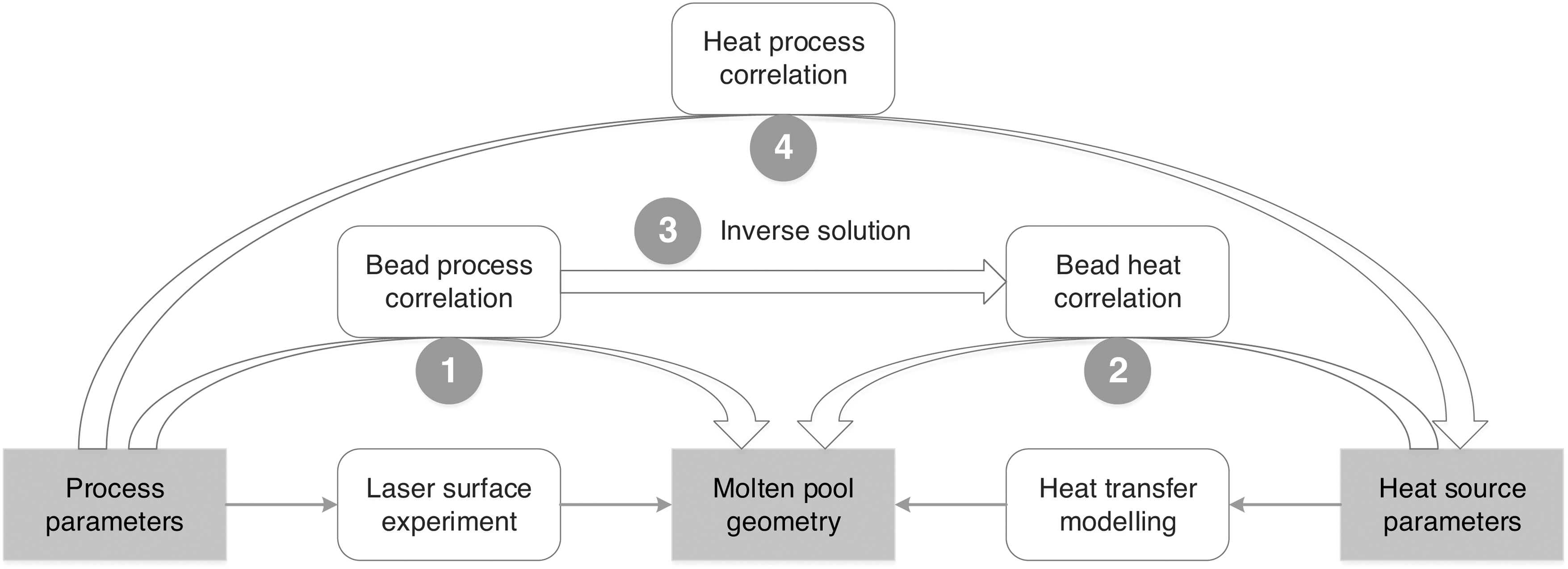
Heat process correlation flowchart.

Experimental

For laser additive manufacturing processes, the powder material is usually applied by pre-placing or coaxial conveying. Taking laser powder-bed fusion, for example, the powder material is pre-placed to form a relatively smooth surface before laser scanning. Furthermore, the physical properties of powder is commonly simplified as the same with those of substrate.³¹ Therefore, such laser additive manufacturing processes are analogous to an assembly of laser surfacing.

As for coaxially supplied powder fusion processes, the effect of material stacking on heat transfer would be insignificant as the amount of new material is comparatively small to the substrate.³² Thus, laser surfacing is utilized in this research for saving experimental and computational cost. Experiment for heat process modeling was carried out on AISI 1045 carbon steel substrates with dimensions of 50 × 24 × 10 mm by laser surfacing. Table 1 illustrates chemical compositions of AISI 1045 carbon steel.

Table 1.

Chemical Composition of AISI 1045 Carbon Steel (wt.%)

C	Si	Mn	S	P	Cr	Fe
0.42–0.5	0.17–0.37	0.5–0.8	<0.035	<0.035	<0.25	Bal.

The laser additive manufacturing system used in this study, as shown in Figure 3, is composed of a Lasermesh FDH0273 laser head, a FANUC M-710iC/50 industrial robot, an IPG high power fibre laser YLS-3000, and a TFLW-4000WDR-01-3385 chiller, and so on. During surfacing, Argon gas of 0.5 MPa is coaxially shielding the substrate surface by the conveying device.

FIG. 3.

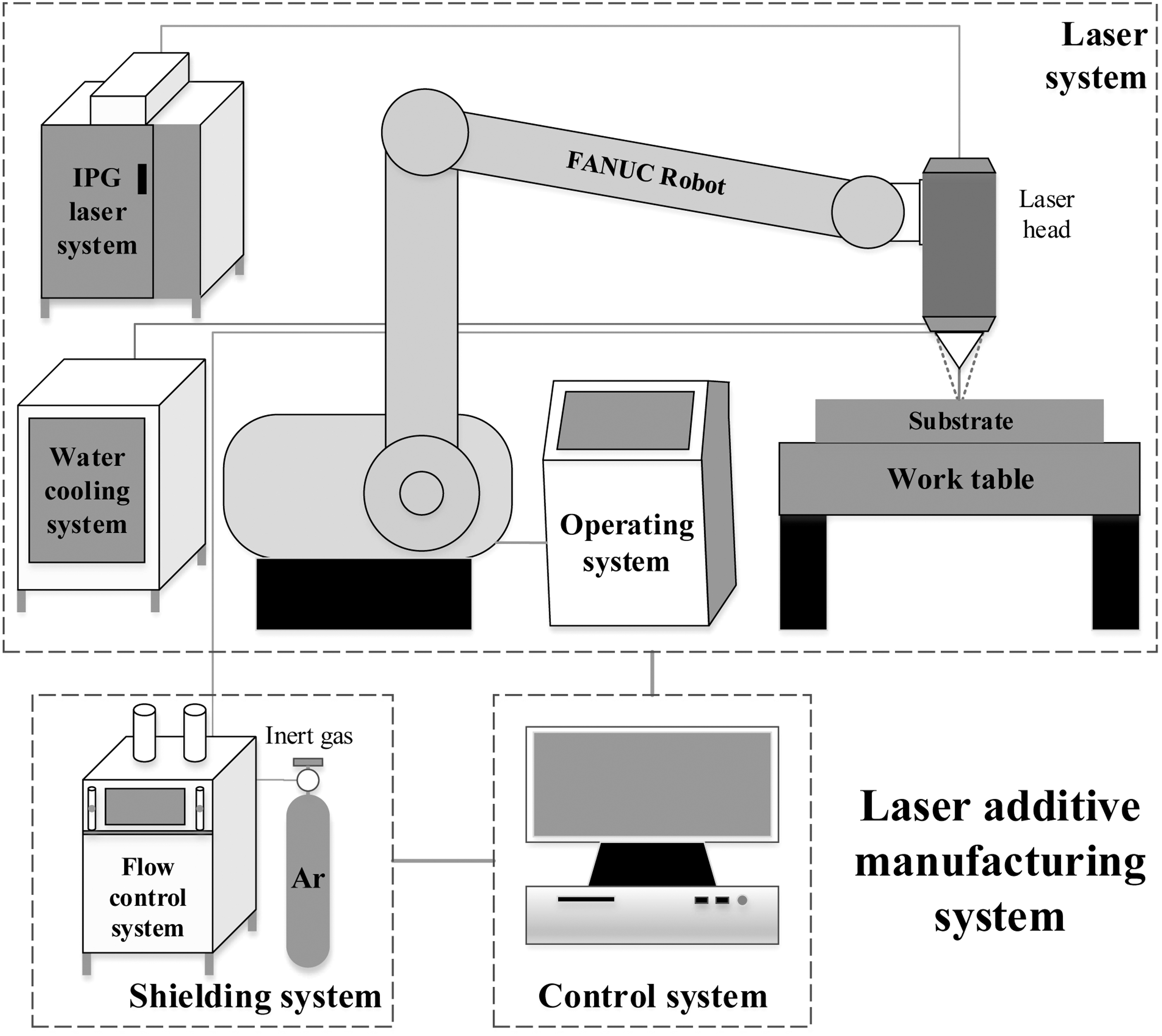
Laser additive manufacturing system.

A three-factor-five-level experimental design matrix, including 14 axial and 6 center points, was proposed using central composite design (CCD), based on RSM in the environment of Design-Expert. Three investigated process parameters are laser power, scanning speed, and defocusing distance. The levels of three parameters are illustrated in Table 2. An alpha level of 1.682 is recommended for the three-factor CCD and the decimal part of actual value is round of for better operation.

Table 2.

Laser Surfacing Parameters and Levels

Parameter	Symbol	Unit	Levels
Parameter	Symbol	Unit	−1.682	−1	0	1	1.682
LP	P	W	864	1000	1200	1400	1536
SS	v	mm·s⁻¹	5	6	8	10	11
DD	D_f	mm	−3	−2	0	2	3

DD, defocusing distance; LP, laser power; SS, scanning speed.

Before laser surfacing, the substrates were cleaned with acetone to remove surface impurities. Then, the substrates were laser surfaced with a single track of 40 mm at the surface center. After laser processing, the specimens were sectioned transversely to the scanning direction, ground and polished for geometrical morphology observation using three-dimensional microscopy system HIROX KH1300. The bead geometry is characterized by three quantities, namely width, depth, and area, as depicted in Figure 4. The characteristics are measured from macromorphology of specimen cross sections using Digimizer software.

FIG. 4.

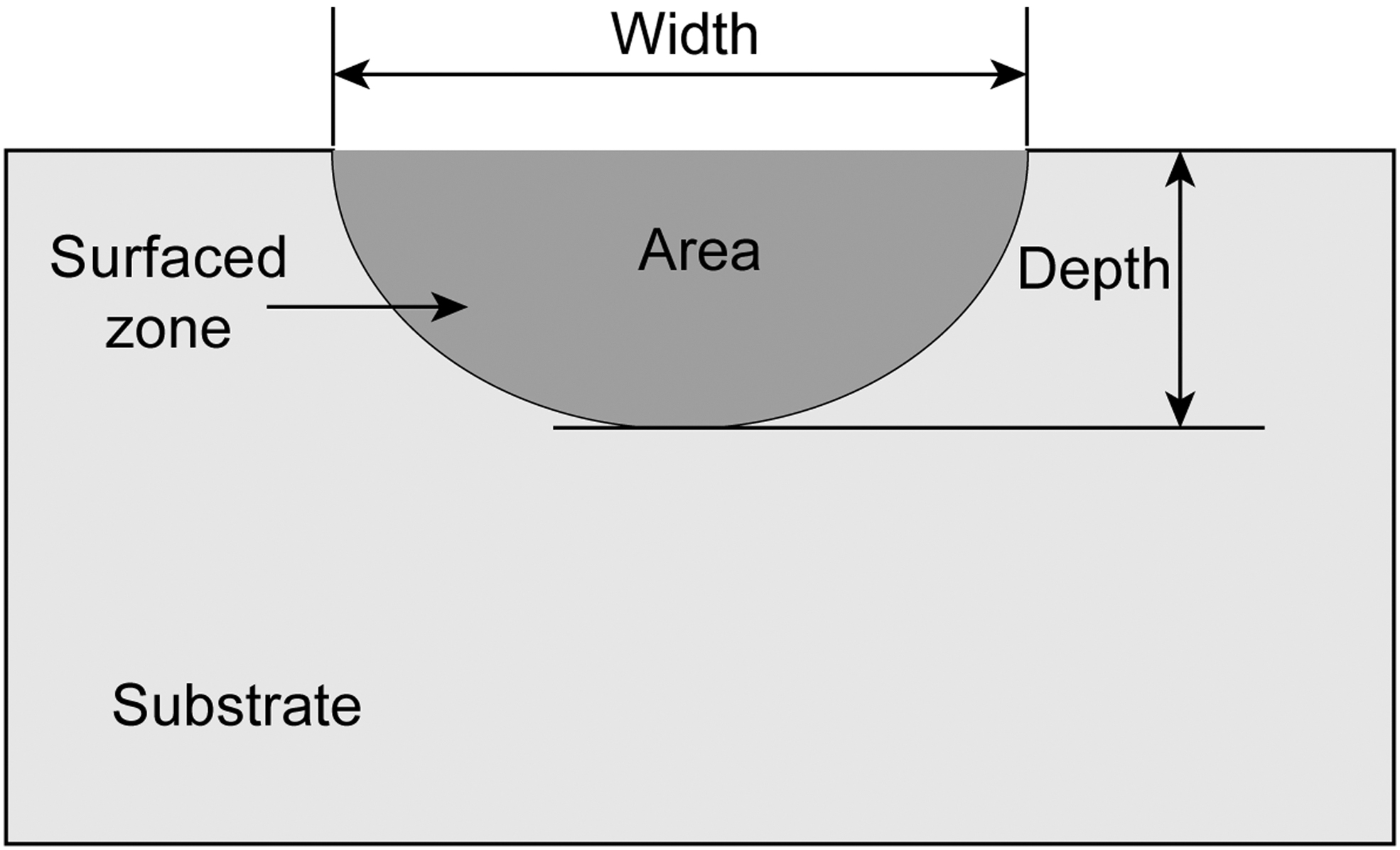
Schematic diagram of bead geometry and characteristics.

Numerical

Numerical simulations of laser surfacing were conducted to understand the effects of heat source coefficients on simulated bead geometry. With correlations established, heat source coefficients can be inversely identified for experimentally applied laser surfacing conditions.

The governing differential equation of heat conduction in the workpiece being laser surfaced is given as follows³³: $k (\frac{\partial^{2} T}{\partial x^{2}} + \frac{\partial^{2} T}{\partial y^{2}} + \frac{\partial^{2} T}{\partial z^{2}}) + \dot{q} = ρ c_{p} \frac{\partial T}{\partial t},$ (3)

where T is temperature, t is time, k is the thermal conductivity, c_p is the specific heat capacity, ρ is the density, and $\dot{q}$ is the rate of heat distributed in the workpiece. The melt pool of laser surfacing is of small size, complicated shape with concentrated energy. Therefore, 3D Gaussian volumetric heat source is selected, as illustrated by Equation (4)³⁴: $\begin{matrix} Q (x, y, z) & = \frac{6 \sqrt{3} η Q_{0}}{π \sqrt{π} r^{2} c} exp (- \frac{3 {(x - x_{0} - v t)}^{2}}{r^{2}} - \frac{3 {(y - y_{0})}^{2}}{r^{2}} \\ - \frac{3 {(z - z_{0})}^{2}}{c^{2}}), \end{matrix}$ (4)

where Q is the Gaussian volumetric heat flux, Q₀ is the heat input in W/mm³, x₀, y₀, and z₀ are the coordinates of heat source center, v is the scanning speed, t is time, and η, r, and c are the coefficients of heat source model. Figure 5 illustrates an example distribution of heat flux at the top surface.

FIG. 5.

Gaussian heat flux distribution at top surface.

Boundary conditions for the simulation include convection and radiation of surfaces exposed to the air. Heat loss due to the boundary conditions is formulated as follows: $k \frac{\partial T}{\partial \vec{n}} = - \in σ (T^{4} - T_{0}^{4}) - h_{c v} (T - T_{0}),$ (5)

where T₀ is the ambient temperature, ϵ is the radiation emissivity of the surface, σ is the Stefan–Boltzmann constant, and h_cv is the convection coefficient. Figure 6 illustrates the boundary conditions applied for numerical simulation. Five points of interest are also marked for tracking thermal history along the scanning direction.

FIG. 6.

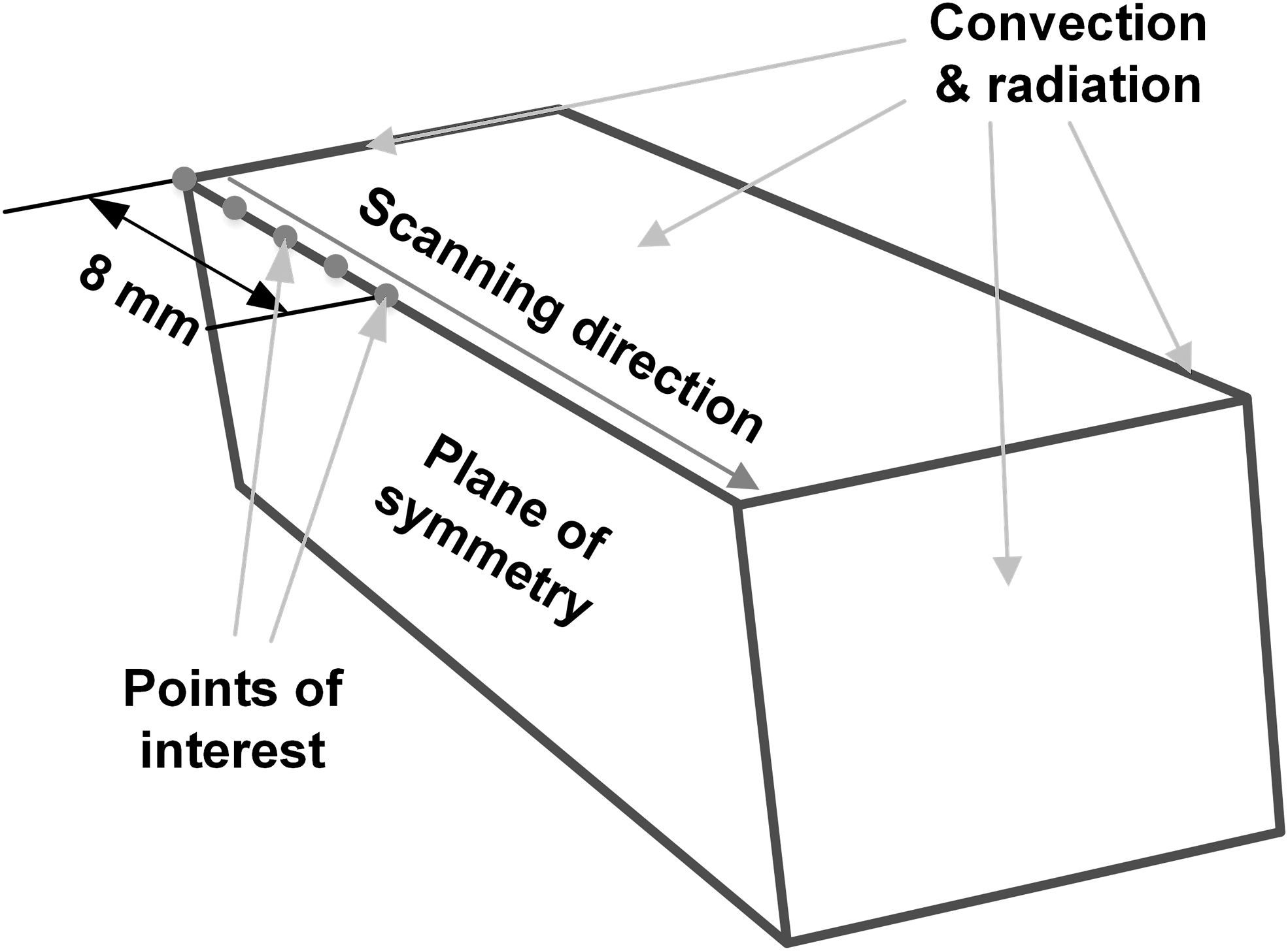
Boundary conditions.

Figure 7 shows the analysis model and moving direction of the laser beam. Owing to geometric symmetry, only half the plate (50 × 12 × 10 mm) was modeled to reduce computation effort. The domain was meshed with 624,000 linear brick elements (DC3D8) in ABAQUS. A finer mesh (0.1 × 0.1 × 0.1 mm) was used for areas in contact with the laser beam since they experienced a complicated thermal sequence of transient heating and cooling. The mesh size was sufficiently small for obtaining convergent calculation results according to literature.^6,21,35,36 A subroutine was created to define the shape and motion of laser heat source.

FIG. 7.

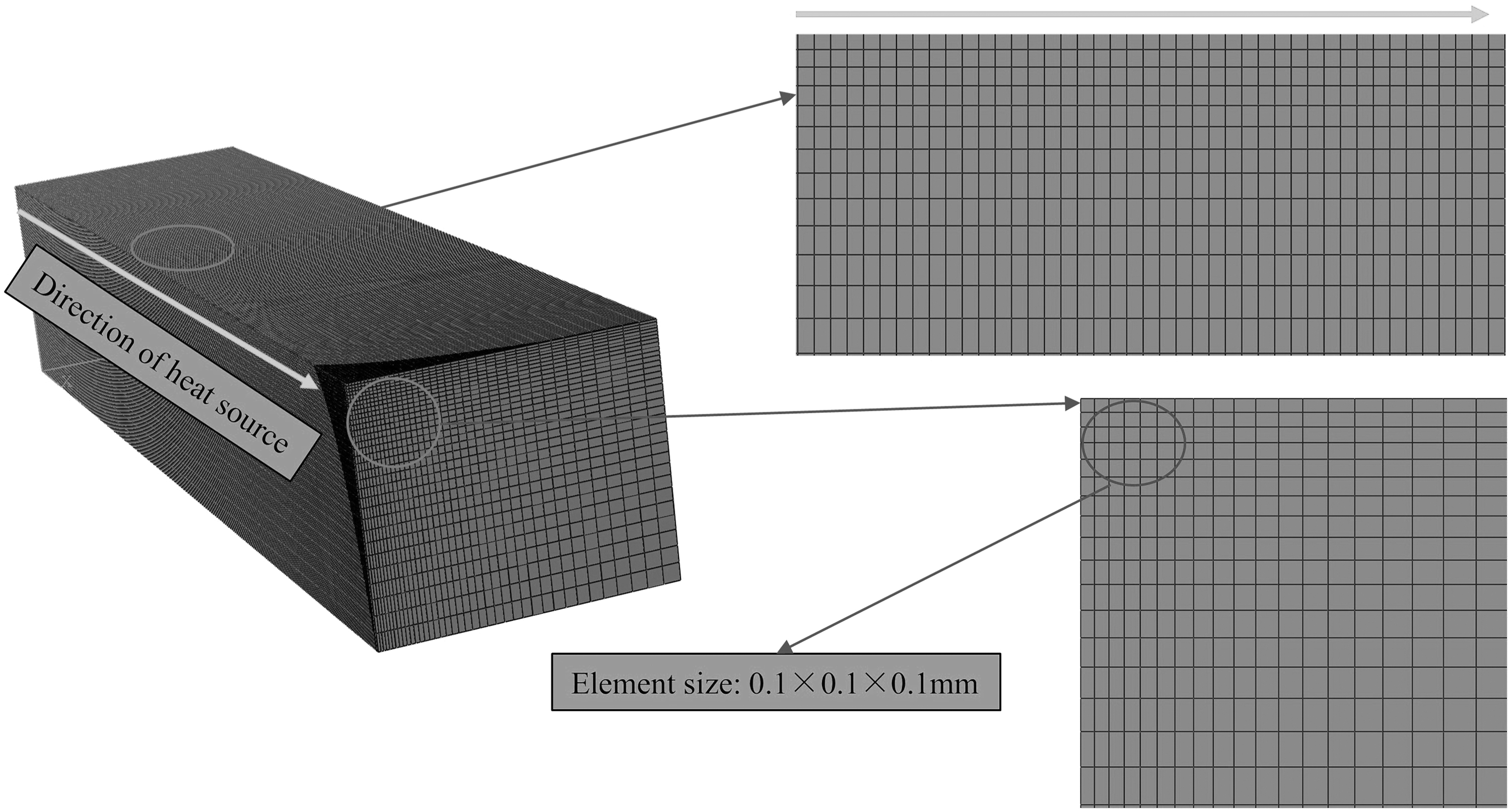
Half-model of the AISI 1045 carbon steel plate.

Temperature-dependent thermal properties of AISI 1045 carbon steel were considered in accordance with literature,^37,38 as shown in Figure 8. The properties out of the data were obtained through linear interpolation. Thermal effects due to melt pool solidification were included using the latent heat of melting (277 J·kg⁻¹) at the respective solidus (1349°C) and liquidus temperatures (1495°C).

FIG. 8.

Thermal physical properties of AISI 1045 steel.

After thermal analysis, temperature data alongside two paths in accordance with the experimentally sectioned position, transversely and vertically, as illustrated in Figure 9, were extracted to obtain the bead geometry. Characteristics of molten pool were identified by positioning the melting point with spline interpolation.

FIG. 9.

Extraction of temperature distributions for bead geometry identification.

To reveal the relationship between heat source parameters and bead geometries, a four-factor-five-level CCD matrix was proposed for simulation runs. Four factors investigated include efficiency of laser power, radius and depth of heat source, and moving velocity of laser. Table 3 illustrates the studied factors and their levels. The simulation matrix consists of 24 axial points and 6 replicate centers. An alpha level of 2 is recommended for this four-factor CCD.

Table 3.

Heat Source Parameters and Levels

Parameter	Symbol	Unit	Levels
Parameter	Symbol	Unit	−2	−1	0	1	2
AE	η	—	0.4	0.6	0.8	1.0	1.2
HR	r	mm	0.3	1.0	1.7	2.4	3.1
HH	c	mm	0.2	0.4	0.6	0.8	1.0
SS	v	mm·s⁻¹	4	6	8	10	12

AE, absorption efficiency; HH, heat height; HR, heat radius.

To reduce computational cost, the effect of laser power is embodied by the absorption efficiency and the value is considered to be constant (1200 W). By applying equivalent effective power, the actual absorption efficiency can be calculated from the designated laser power. In addition, the process factor defocusing distance is not explicitly embodied in finite element simulation. Its effect on thermal cycling of manufacturing process is included in resulted heat source and will be revealed by process-heat correlation later. Therefore, defocusing distance is not investigated and excluded from this CCD.

Results and Discussion

After laser surface processing and simulation, response results were obtained for respective experimental and numerical runs. The effects of processing parameters and heat source coefficients on experimental and simulated bead geometry were investigated by analysis of variances (ANOVAs), respectively. Afterward, heat model coefficients were identified inversely for every setting of laser surfacing conditions to understand heat process correlation.

Bead process correlations

Table 4 lists the detailed experimental runs and corresponding response results for bead process correlations. With the data, multiple regression can be conducted to map the processing parameters to experimental bead geometry characteristics.

Table 4.

Central Composite Design Matrix and Responses for Laser Surfacing

Run	P, W	v, mm·s ⁻¹	D_f, mm	Width, mm	Depth, mm	Area, mm²
1	1200	8	0	2.559	0.899	1.613
2	1400	6	2	2.886	1.149	2.375
3	1400	10	−2	2.464	0.886	1.525
4	1000	6	2	2.632	0.797	1.503
5	1000	10	−2	2.191	0.591	0.924
6	1000	10	2	2.337	0.613	1.008
7	1400	6	−2	2.715	1.092	2.115
8	1200	11	0	2.400	0.772	1.274
9	1200	8	0	2.480	0.895	1.616
10	1000	6	−2	2.407	0.746	1.259
11	1400	10	2	2.667	0.899	1.661
12	1536	8	0	2.740	1.076	2.077
13	1200	8	0	2.562	0.886	1.603
14	1200	8	0	2.540	0.860	1.510
15	1200	8	0	2.502	0.854	1.490
16	1200	8	0	2.477	0.864	1.502
17	1200	5	0	2.762	1.067	2.093
18	864	8	0	2.273	0.594	0.947
19	1200	8	3	2.651	0.883	1.638
20	1200	8	−3	2.438	0.826	1.369

The correlation between geometry characteristics of hardened layer and processing parameters are summarized in Equation (6), as follows:

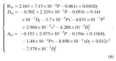
Table 5 illustrates the fitting statistics of bead process correlations. From the table, determination coefficients R² and adjusted R² for three characteristics all approximate to 1. Furthermore, the differences between adjusted R² and predicted R² (0.009, 0.05, and 0.0085) are all <0.2. Therefore, the models have good capacity of prediction. Adequate precisions are >40, indicating that the models have good resolution and would exhibit enough resilience to errors. Figure 10 compares the model predicted bead geometry characteristics with experimental counterparts. The close surrounding of data points to the line y = x indicates the good accuracy of prediction.

FIG. 10.

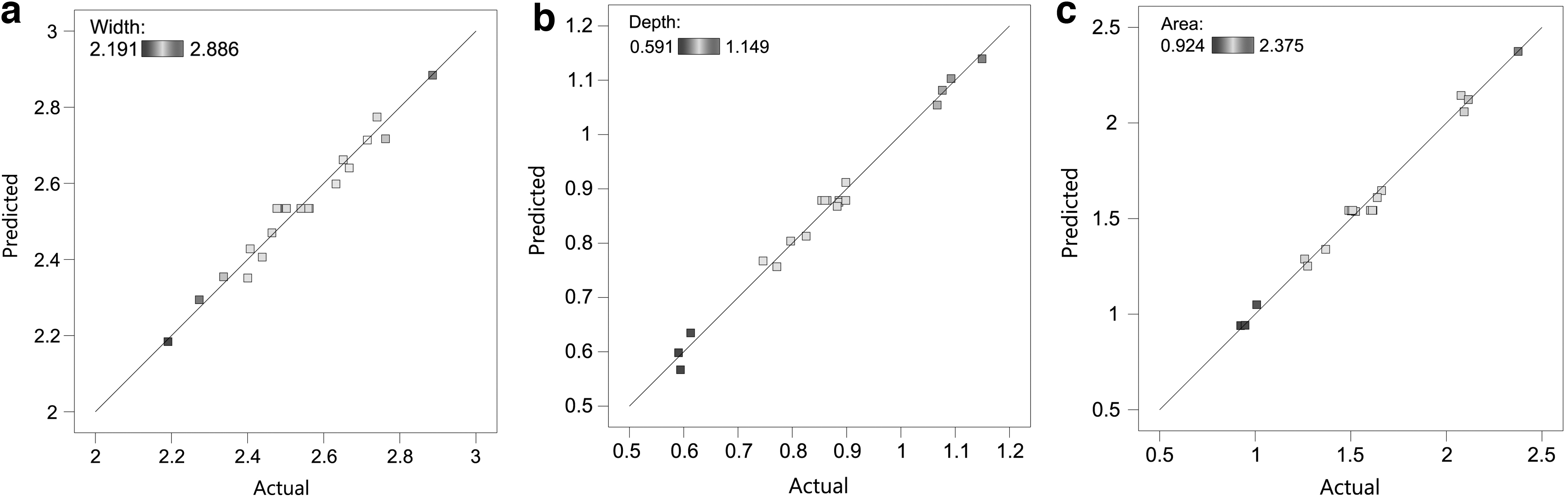
Comparison of predicted bead geometry characteristics to experimental data. (a) Width; (b) depth; (c) area.

Table 5.

Fitting Statistics for Bead Process Correlation

Model	R ²	Adjusted R²	Predicted R²	Adequate precision
W _ex	0.9676	0.9615	0.9525	45.8900
D _ex	0.9893	0.9831	0.9633	44.5294
A _ex	0.9888	0.9823	0.9738	43.9224

Figure 11 shows the influences of process parameters on bead geometry characteristics. Figures 12 –14 illustrate the cross-sectional morphologies due to varied process factors. From the figures, one can tell that all three geometry characteristics of hardened layer are related to laser power, scanning speed, and defocusing distance. The increase in laser power, and/or decrease in scanning speed lead to increase in bead geometry. This is due to the increased specific energy melts more volume of the substrate. As applied laser is defocused from focal length, the energy intensity is dispersed from center to side. With enough heat input, wider and deeper melt pools are resulted with great transverse cross-sectional areas.

FIG. 11.

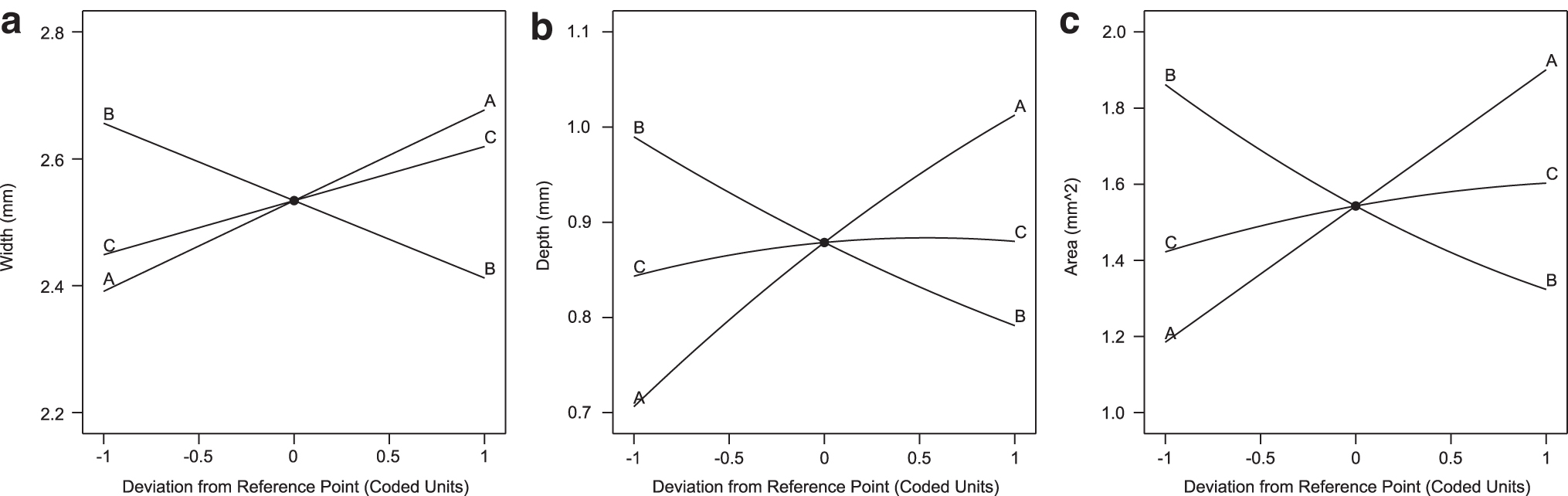
Perturbation of process factors on bead geometry characteristics (A: LP; B: SS; C: DD). (a) Width; (b) depth; (c) area. DD, defocusing distance; LP, laser power; SS, scanning speed.

FIG. 12.

Cross-sectional morphology of experimental specimens with varied laser power (v = 8 mm·s⁻¹, D_f = 0 mm). (a) P = 864 W; (b) P = 1200 W; (c) P = 1536 W.

FIG. 13.

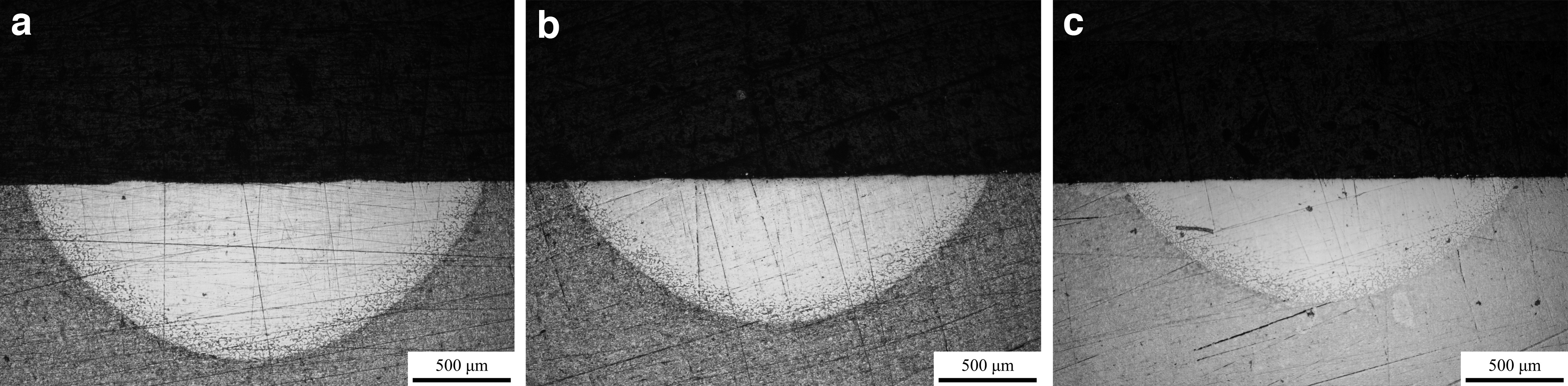
Cross-sectional morphology of experimental specimens with varied scanning speed (P = 1200 W, D_f = 0 mm). (a) v = 5 mm·s⁻¹; (b) v = 8 mm·s⁻¹; (c) v = 11 mm·s⁻¹.

FIG. 14.

Cross-sectional morphology of experimental specimens with varied defocusing distance (P = 1200 W, v = 8 mm·s⁻¹). (a) D_f = ⁻3 mm; (b) D_f = 0 mm; (c) D_f = 3 mm.

However, when the laser beam is defocused beneath the substrate (negative distance of focusing), it is in a convergent manner along propagation direction, leading to a larger portion of reflection than that of the corresponding positive position and thus reduction of heat input.³⁹ The melt pool thereby becomes shallower and narrower due to more convergent distribution of heat flux. Table 6 ranks the influence of process parameters on the width, depth, and area of melt pools. From the table, rankings of three factors on bead geometry characteristics are the same, that is, P > v > D_f. This indicates that linear heat input is the most significant factor influencing bead geometry.

Table 6.

Factor Importance Ranking for Bead Process Correlation

Model	P	v	D_f
W _ex	1	2	3
D _ex	1	2	3
A _ex	1	2	3

Bead heat correlations

Figure 15 depicts the temperature history of laser surfacing process for the condition of center point. From the figure, one can find that the laser beam melts the substrate surface soon after the heat input is applied (Fig. 15a). As the heat source moves forward, as shown in Figure 15b–e, the temperature of melt pool is continuously elevated from 3060°C to 3270°C at t = 1.618 s and the substrate behind the heat source starts to cool down from the melting temperature.

FIG. 15.

Thermal history of laser surfacing at center point condition. (a) t = 0.169 s; (b) t = 0.506 s; (c) t = 1.036 s; (d) t = 1.301 s; (e) t = 1.618 s; (f) t = 2.042 s; (g) t = 2.360 s; (h) t = 2.625 s; (i) t = 2.996 s; (j) t = 3.420 s; (k) t = 4.002 s; (l) t = 4.320 s.

Then, the melt pool is gently heated up to ∼3275°C (Fig. 15f–i) and the heat input is transferred down to the substrate bottom after enough thermal accumulation. The melt pool achieves stable temperature at around t = 3.42 s, that is, T = 3276°C, as depicted in Figure 15j–l. During the entire thermal cycle, only a small fraction is heated up to be >600°C, which explains the resulted small heat-affected zone.

The thermal cycles of specific points, as illustrated in Figure 16, also demonstrate such an observation. The positions along scanning direction get heated up sequentially. The maximum temperature is obtained after travel of about 4 mm. A steep heating and cooling rate are achieved within about 0.5 s.

FIG. 16.

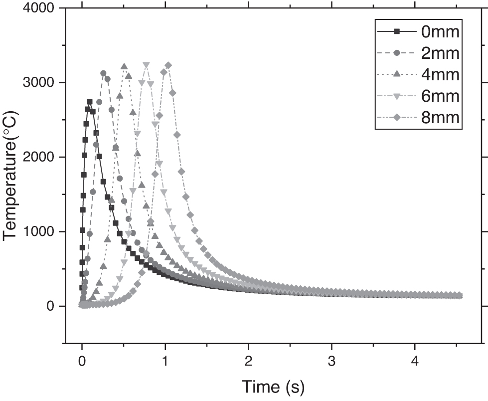
Thermal cycles of five points with distances from scanning origin (Fig. 6) at center condition (η = 0.8, r = 1.7, c = 0.6, and v = 8).

Table 7 illustrates the results of thermal analysis simulations. Multiple regression is then applied to understand the influences of heat source coefficients on simulated bead geometry.

Table 7.

Central Composite Design Matrix and Responses for Bead Heat Correlation

Run	η	r, mm	c, mm	v, mm·s ⁻¹	Width, mm	Depth, mm	Area, mm²
1	0.4	1.7	0.6	8	1.028	0.283	0.222
2	1	1	0.8	6	3.138	1.509	3.702
3	0.8	0.3	0.6	8	2.203	1.167	2.028
4	0.8	1.7	0.2	8	2.936	0.971	2.132
5	0.6	1	0.8	6	2.205	1.027	1.762
6	0.6	2.4	0.4	6	2.178	0.491	0.810
7	0.6	1	0.4	10	2.090	0.844	1.370
8	0.6	2.4	0.8	6	1.814	0.507	0.702
9	1	2.4	0.8	6	3.553	1.196	3.254
10	1	1	0.4	10	2.821	1.256	2.780
11	0.6	1	0.4	6	2.284	0.953	1.682
12	0.6	1	0.8	10	1.988	0.918	1.406
13	0.8	1.7	0.6	12	2.512	0.861	1.654
14	0.8	1.7	1	8	2.650	1.063	2.182
15	1	1	0.8	10	2.796	1.335	2.914
16	1	2.4	0.8	10	3.052	0.962	2.238
17	0.8	1.7	0.6	4	3.214	1.222	3.012
18	1	1	0.4	6	3.125	1.421	3.480
19	0.8	1.7	0.6	8	2.798	1.001	2.108
20	0.8	1.7	0.6	8	2.798	1.001	2.108
21	0.8	1.7	0.6	8	2.798	1.001	2.108
22	0.6	2.4	0.4	10	1.686	0.339	0.430
23	1	2.4	0.4	6	3.697	1.154	3.196
24	0.6	2.4	0.8	10	1.151	0.303	0.266
25	0.8	1.7	0.6	8	2.798	1.001	2.108
26	0.8	1.7	0.6	8	2.798	1.001	2.108
27	0.8	1.7	0.6	8	2.798	1.001	2.108
28	1	2.4	0.4	10	3.243	0.929	2.272
29	1.2	1.7	0.6	8	3.629	1.462	4.130
30	0.8	3.1	0.6	8	2.244	0.488	0.792

The correlation between geometry characteristics of melt pool and heat source coefficients are summarized in Equation (7):

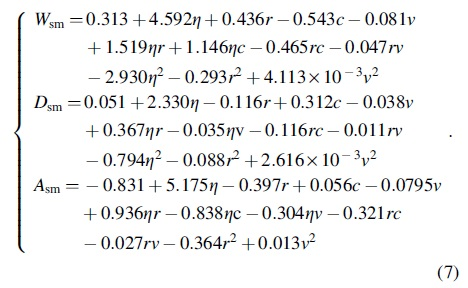
From Table 8, the determination coefficients R² and adjusted R² for three characteristics all approximate to 1. Furthermore, the disparity of predicted R² from adjusted R² (0.0061, 0.0133, and 0.0042) are much <0.2. Therefore, the established heat bead relationships have good capacity of prediction. Adequate precisions are all >4, indicating that the models have good resolution and would exhibit enough resilience to errors. Comparisons of model predicted bead geometry characteristics to simulated data, as illustrated in Figure 17, also demonstrate the good accuracy of prediction.

FIG. 17.

Comparison of predicted bead geometry characteristics to simulated data. (a) Width; (b) depth; (c) area.

Table 8.

Fitting Statistics for Bead Heat Correlation

Model	R ²	Adjusted R²	Predicted R²	Adequate precision
W _sm	0.9969	0.9951	0.9890	92.2457
D _sm	0.9954	0.9926	0.9793	65.2864
A _sm	0.9984	0.9974	0.9934	118.2204

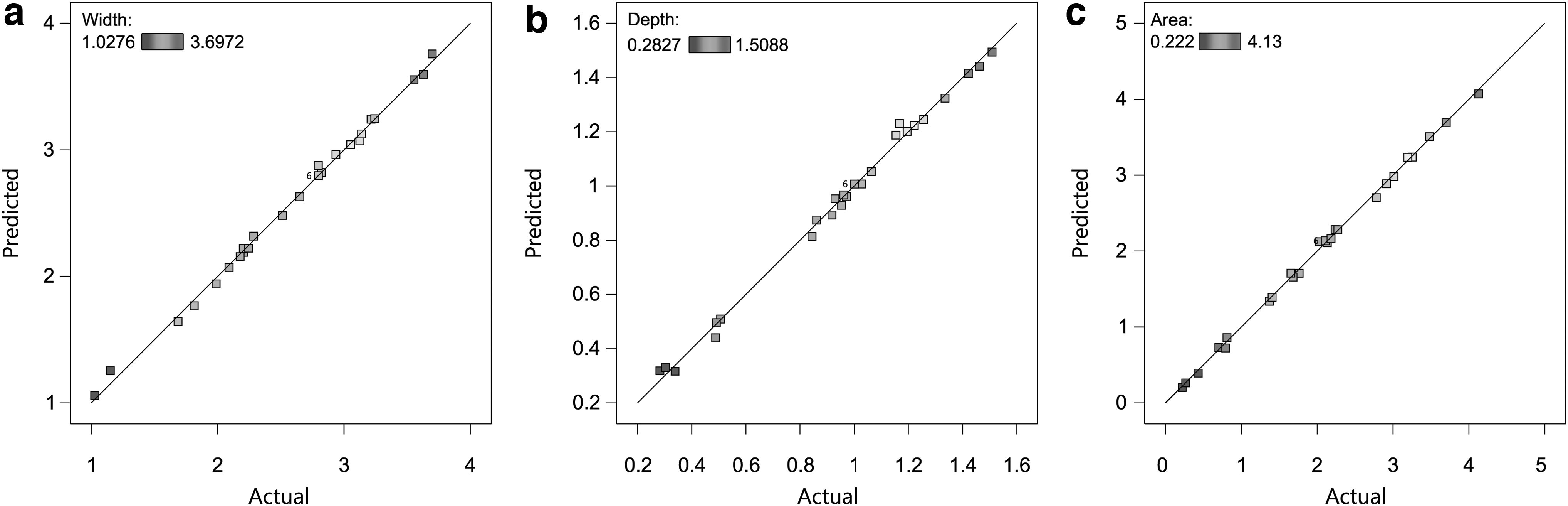
Figures 18 –20 show the cross-sectional thermal fields due to varied heat source parameters, respectively. From the figures, one can find that the melt pool is determined by all the heat source coefficients. Specifically, as the efficiency increases, the melt pool is broadened and deepened dramatically at first and then tends to be steady. The reason is straightforward that the applied laser power increases as the efficiency is improved. The elevated heat input thus melts more material to obtain wider and deeper melt pool.

FIG. 18.

Cross-sectional thermal fields due to varied efficiency (r = 1.7 mm, c = 0.6 mm, and v = 8 mm·s⁻¹).

FIG. 19.

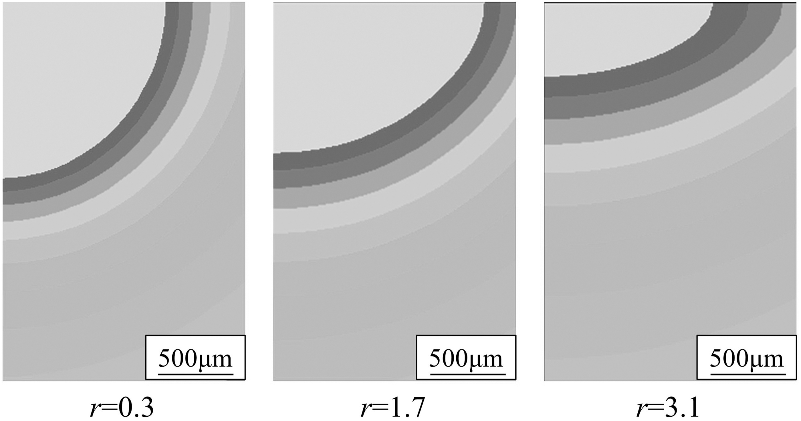
Cross-sectional thermal fields due to varied radius (η = 0.8, c = 0.6 mm, and v = 8 mm·s⁻¹).

FIG. 20.

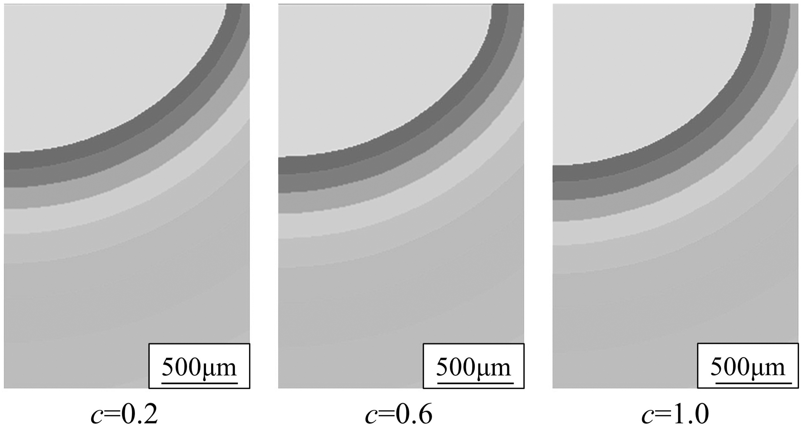
Cross-sectional thermal fields due to varied height (η = 0.8, r = 1.7 mm, and v = 8 mm·s⁻¹).

However, the increased energy is mainly exerted around the center of heat source, according to Equation (4), its effect on heating subsurface material would be dramatically reduced. As the radius increases, the melt pool gets shallower, but the pool width increases first and decreases afterward. This is because increase of radius stretches the power distribution and reduces the gradient between center and perimeter. Excessive increment of radius would result in larger area of insufficient energy density, thus reducing the width of melt pool. With increase in heat height, the melt pool gently becomes narrower and deeper as the heat input is stretched toward the substrate interior.

Figure 21 also illustrates the effects of heat source coefficients on the bead geometry characteristics. From the figure, it can be found that the simulated bead geometry is determined by four factors. Specifically, increase in absorption efficiency and/or decrease in scanning speed lead to an enlarged bead geometry. Increment of heat source radius results in decreased depth and area, but has little effect on the width. As the height of heat source gets increased, the laser beam penetrates deeper with a smaller width and, therefore, the area is almost not affected.

FIG. 21.

Perturbation of heat source coefficients on bead geometry characteristics (A: AE; B: HR; C: HH; D: SS). (a) Width; (b) depth; (c) area. AE, absorption efficiency; HH, heat height; HR, heat radius.

The reason is that the efficiency of laser absorption and scanning speed determine the specific heat input into the substrate. Radius and height of heat source reflect the distribution breadth and depth of laser energy. The importance ranking of parameter influence on simulated melt pool geometry is summarized in Table 9. From the table, absorption efficiency and radius of heat are the most important two factors affecting the width, depth, and area of weld bead, followed by scanning speed and heat height.

Table 9.

Factor Importance Ranking for Bead Heat Correlation

Model	η	r	c	v
W _sm	1	4	3	2
D _sm	1	2	4	3
A _sm	1	2	4	3

Heat process correlations

According to the response models established in the previous section, the heat source coefficients can be resolved in accordance with the experimental measurements of bead geometry. Thereafter, the relationships between heat source coefficients and process parameters are readily established through regression analysis.

Inverse solution of heat source coefficients

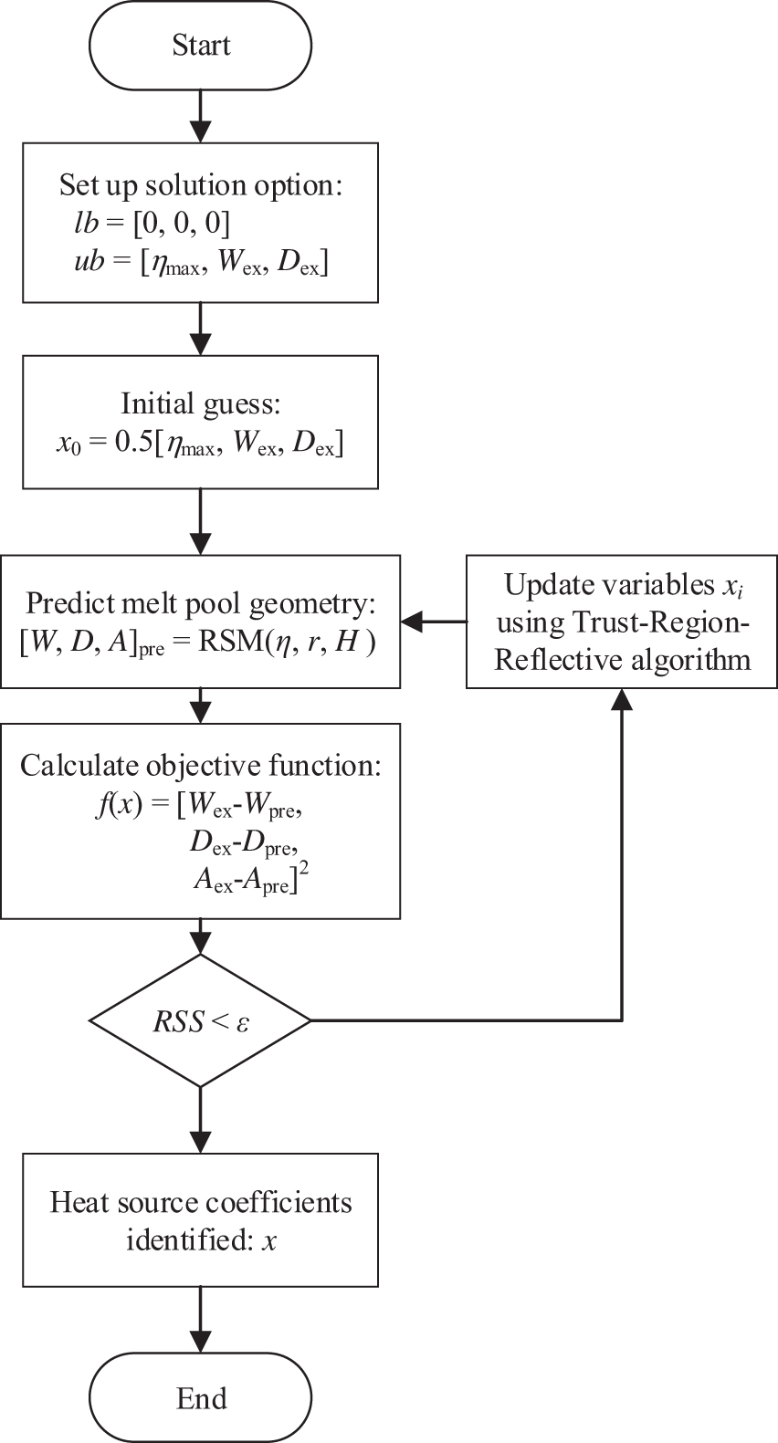
The inverse solution was performed using the trust-region-reflective nonlinear least square algorithm in MATLAB environment, as depicted in Figure 22. The lower bound was set to be zero for three coefficients, that is, lb = [0, 0, 0]. The upper bound was reasonably assumed to be correlated with experimental bead geometry, namely $u b = [η_{m a x} = \frac{P}{1200}, W_{e x}, D_{e x}]$ . Because the simulation data show that heat radius and height are both less than the corresponding width and depth of weld bead. Therefore, the upper bounds of r and c can be assigned as W_ex and D_ex, respectively.

FIG. 22.

Inverse solution flowchart for heat source coefficients.

In addition, 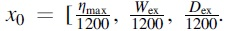$η_{m a x} = \frac{P}{1200}$ indicates 100% absorption of laser for the applied experimental power. The initial guess was then set as half the upper bound, that is,

Using the initial guess, the bead heat models were used to predict the melt pool geometry for the current set of heat source coefficients. The inverse approach minimized the error between experimental and predicted melt pool geometry. The objective function, f (x), is the squared two-norm of the residual error: $f (x) = {[\begin{matrix} W_{e x} - W_{p r e} \\ D_{e x} - D_{p r e} \\ A_{e x} - A_{p r e} \end{matrix}]}^{2} .$ (8)

Upon the stop criteria being met, the optimum heat source coefficients were obtained. The procedure was repeated for all the experimental runs. The results are illustrated in Table 10. Therefore, the effects of process factors on heat source coefficients are investigated and their correlations established in the following section.

Table 10.

Heat Source Coefficients Calibrated for Laser Surfacing

Run	P, W	v, mm·s⁻¹	D_f, mm	η	r, mm	c, mm
1	1200	8	0	0.6754	1.4020	0.2518
2	1400	6	2	0.6561	1.2688	0.4068
3	1400	10	−2	0.5973	1.3672	0.2885
4	1000	6	2	0.7469	1.7301	0.1795
5	1000	10	−2	0.7438	1.9201	0.1896
6	1000	10	2	0.7870	2.0071	0.1455
7	1400	6	−2	0.6102	1.1405	0.3671
8	1200	11	0	0.6829	1.6426	0.1992
9	1200	8	0	0.6649	1.2615	0.2917
10	1000	6	−2	0.6796	1.6040	0.2071
11	1400	10	2	0.6478	1.6019	0.2424
12	1536	8	0	0.6055	1.2448	0.4073
13	1200	8	0	0.6752	1.4403	0.2521
14	1200	8	0	0.6594	1.4623	0.2120
15	1200	8	0	0.6497	1.4105	0.2110
16	1200	8	0	0.6478	1.3635	0.2313
17	1200	5	0	0.6774	1.2415	0.3379
18	864	8	0	0.7942	1.8257	0.1018
19	1200	8	3	0.6958	1.5831	0.2397
20	1200	8	−3	0.6328	1.4905	0.2553

Effects of process factors on efficiency of heat source

The response model correlating absorption efficiency with laser surfacing parameters is depicted in Equation (9): $\begin{matrix} η & = 1.1915 - 0.7565 \times 1 0^{- 3} P + 0.01953 v + 0.01202 D_{f} \\ - 3.9177 \times 1 0^{- 5} P v + 3.2935 \times 1 0^{- 7} P^{2} \\ + 1.9459 \times 1 0^{- 3} v^{2} \end{matrix} .$ (9)

The partial derivatives of efficiency to three factors are identified as follows: $\{\begin{matrix} \frac{\partial η}{\partial P} = - 0.7565 \times 10^{- 3} - 3.9177 \times 10^{- 5} v + 6.587 \times 10^{- 7} P \\ \frac{\partial η}{\partial v} = 0.01953 - 3.9177 \times 10^{- 5} P + 3.8918 \times 10^{- 3} v \\ \frac{\partial η}{\partial D_{f}} = 0.01205 \end{matrix} .$ (10)

From Equation (9), one can find that the absorption efficiency is a parabola function of laser power, scanning speed, and defocusing distance. Equation (10) shows that the influence of laser power on absorption efficiency is also affected by scanning speed. The smaller the scanning speed, the greater the increase of efficiency with increasing power applied, vice versa. The derivative of efficiency to defocusing distance indicates a proportional relationship between them.

Table 11 illustrates the ANOVA result for absorption efficiency of laser. From the table, the p-value of selected model for the response absorption efficiency of laser beam is <0.01%, and the counterpart for lack of it (87.95%) is much >5%, which suggests that the selected items in the response model play significant roles and the lack of fitness is probably introduced by random error. The coefficients of determination, R², adjusted R², and predicted R² are all >0.95. In addition, the difference between adjusted R² and predicted R² (0.0128) is <0.2.

Table 11.

Analysis of Variance for Absorption Efficiency (η)

Source	Sum of squares	df	Mean square	F	p, Prob>F
Model	0.0556	6	0.0093	101.62	<0.0001	Significant
P	0.0426	1	0.0426	467.67	<0.0001
v	0.0007	1	0.0007	7.34	0.0179
Df	0.0073	1	0.0073	79.69	<0.0001
P_v	0.0020	1	0.0020	21.55	0.0005
P ²	0.0025	1	0.0025	27.79	0.0002
v ²	0.0006	1	0.0006	6.84	<0.0214
Residual	0.0012	13	0.0001
Lack of it	0.0005	8	0.0001	0.4012	0.8795	Not significant
Pure error	0.0007	5	0.0001
Cor total	0.0568	19
Std. Dev.		0.0095		R ²		0.9791
Mean		0.6765		Adjusted R²		0.9695
C.V. %		1.41		Predicted R²		0.9567
PRESS		0.0025		Adequate precision		35.1401

C.V. %, coefficient of variation.

These indicate that sufficient fitting of experimental data has been accomplished by the response model, together with good prediction capacity. An adequate precision of 35.1401 means high resolution of the established efficiency model with little influence by errors. Figure 23a compares model predicted absorption efficiency with actual values. As the points are closely surrounding the straight line y = x, the absorption efficiency model has good prediction capacity. Therefore, the established response surface model for absorption efficiency has proven good fitting and prediction capacity.

FIG. 23.

Model-related statistics graphs for η. (a) Predicted versus actual; (b) perturbation; (c) contour line of η w.r.t AB; (d) 3D response surface of η to AB.

It can also be found from Table 11 that the absorption efficiency is mainly determined by laser power and scanning speed, followed by defocusing distance. The response is also affected by the interactions P_v and quadratic terms P², v². Figure 23b illustrates the effects of process factors on the absorption efficiency. According to the figure, with decrease in laser power, increase in scanning speed and/or defocusing distance, laser energy is increasingly absorbed by the substrate.

Figure 23c and d shows interaction effects of laser power and scanning speed on the absorption efficiency. It can be observed that as scanning speed increases, the absorption of laser beam becomes more sensitive to laser power. As shown in Equation (10), the partial derivative of η to P is negatively linear with scanning speed. This is probably due to that the absorption of substrate is determined by its thermal capacity.

With increase in scanning speed, the specific energy is dramatically reduced to a lower level. The substrate becomes more capable of absorbing laser power. Therefore, the efficiency is getting greater as laser power increases. When travelling with lower speed, the specific energy input into substrate is relatively high. More laser beams would be radiated into ambient environment rather than being input into the substrate.

Effects of process factors on heat source radius

The relationship between heat source radius and laser surfacing parameters is depicted in Equation (11): $\begin{matrix} r & = 4.261 - 4.641 \times 1 0^{- 3} P + 0.0702 v + 0.0286 D_{f} \\ + 1.497 \times 1 0^{- 6} P^{2} + 0.0202 v^{2} . \end{matrix}$ (11)

The partial derivatives of radius to three factors are identified as follows: $\{\begin{matrix} \frac{\partial r}{\partial P} = - 4.641 \times 10^{- 3} + 2.994 \times 10^{^{_{- 6}}} P \\ \frac{\partial r}{\partial v} = 0.0702 + 0.0404 v \\ \frac{\partial r}{\partial D_{f}} = 0.0286 \end{matrix} .$ (12)

Equation (11) indicates that the heat source radius is also a parabola function of three process parameters. As depicted in Equation (12), the heat source radius is independently affected by three variables. The greater the laser power/scanning speed, the greater the derivative of radius. The defocusing distance still has a proportional influence on the radius.

Table 12 shows the result of ANOVA for heat source radius. From the table, the p-value of selected response model for heat source radius is <0.01%, and the value for lack of fit reaches 53.61%, indicating that adopted items in the response model are significant and the lack of fitness is probably due to random error. The coefficients of determination, R², adjusted R², and predicted R², all approximate to 1. Furthermore, the value of predicted R² is only 0.09 smaller than adjusted R². These suggest that sufficient fitting of experimental data has been accomplished by the response model as well as good predication capacity.

Table 12.

Analysis of Variance for Heat Source Radius (r)

Source	Sum of squares	df	Mean square	F	p, Prob>F
Model	1.00	5	0.2001	39.48	<0.0001	Significant
P	0.5990	1	0.5990	118.15	<0.0001
v	0.2463	1	0.2463	48.58	<0.0001
D_f	0.0409	1	0.0409	8.07	0.0131
P ²	0.0524	1	0.0524	10.33	0.0062
$D_{f}^{2}$	0.0670	1	0.0670	13.21	0.0027
Residual	0.0710	14	0.0051
Lack of it	0.0454	9	0.0050	0.9885	0.5361	Not significant
Pure error	0.0255	5	0.0051
Cor total	1.07	19
Std. Dev.		0.0712		R ²		0.9338
Mean		1.50		Adjusted R₂		0.9101
C.V. %		4.75		Predicted R₂		0.8217
PRESS		0.1911		Adequate precision		20.8770

An adequate precision of 20.8770 means high resolution of the established heat source radius model to differentiate errors. The model predicted responses are compared with actual values in Figure 24a. As the points are close to the straight line y = x, little divergence is observed between predicted and actual values. Therefore, the heat source radius model has been rendered with good fitting and prediction capacity.

FIG. 24.

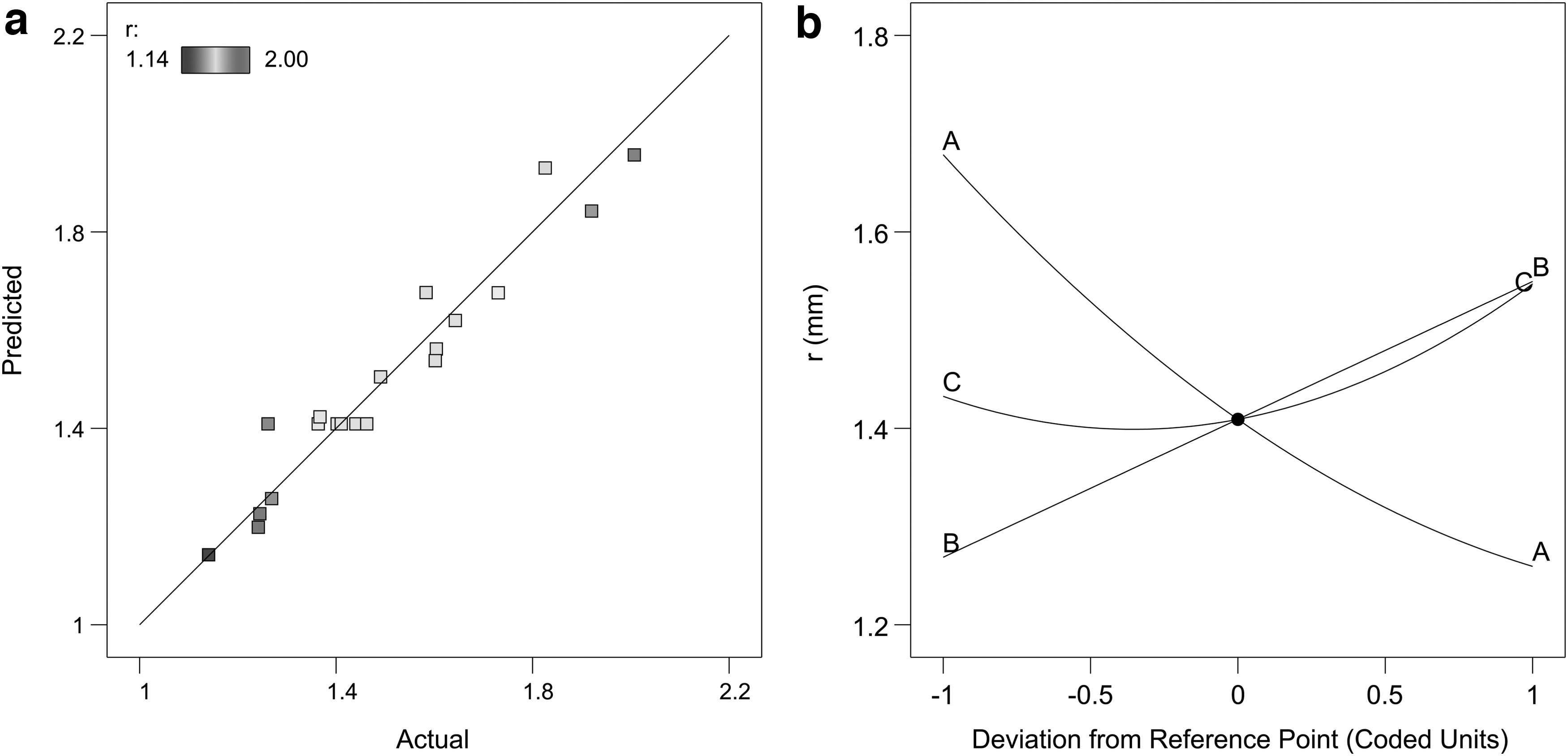
Model-related statistics graphs for r. (a) Predicted versus actual; (b) perturbation.

From Table 12, the heat source radius is determined by all three process factors. The response is also affected by quadratic terms P², $D_{f}^{2}$ without any interaction effects. Figure 24b shows individual influences of three factors on the response. It can be observed that heat source radius is positively linear with scanning speed, but almost negatively proportional to laser power. In addition, the response is a concave function of defocusing distance.

Effects of process factors on heat source depth

The correlation between heat source depth and process factors is shown in Equation (13). $c = - 0.6449 + 8.80 \times 1 0^{- 4} P + 0.0517 v - 6.0 \times 1 0^{- 5} P v .$ (13)

The partial derivatives of the response to influencing factors are deducted as follows: $\{\begin{matrix} \frac{\partial c}{\partial P} = 8.80 \times 10^{- 4} - 6.0 \times 10^{- 5} v \\ \frac{\partial c}{\partial v} = 0.0517 - 6.0 \times 10^{- 5} P \end{matrix} .$ (14)

Equation (13) illustrates that the heat source depth is only relevant with laser power and scanning speed. As can be found from Equation (14), the heat source depth is affected by coupling of these two parameters. The greater the laser power/scanning speed, the smaller the derivative of depth to the other variable. The defocusing distance has no significant influence on the depth.

The ANOVA result for the depth of heat source is illustrated in Table 13. From the table, the p-value of selected model for the response heat source depth is <0.01% and the counterpart for lack of fit is as great as 79.26%, which suggests that the selected items in the response model play significant effects and the lack of fitness is probably introduced by random error. The coefficients of determination, R², adjusted R², and predicted R² are all close to 1. In addition, the predicted R² is only 0.0346 less than the adjusted R².

Table 13.

Analysis of Variance for Heat Source Depth (c)

Source	Sum of squares	df	Mean square	F	p, Prob>F
Model	0.1129	3	0.0376	57.15	<0.0001	Significant
P	0.0881	1	0.0881	133.81	<0.0001
v	0.0202	1	0.0202	30.69	<0.0001
P_v	0.0046	1	0.0046	6.96	0.0179
Residual	0.0105	16	0.0007
Lack of it	0.0059	11	0.0005	0.5767	0.7926	Not significant
Pure error	0.0046	5	0.0009
Cor total	0.1234	19
Std. Dev.		0.0257		R ²		0.9146
Mean		0.2509		Adjusted R²		0.88986
C.V. %		10.23		Predicted R²		0.8640
PRESS		0.1513		Adequate precision		24.3560

Thus, sufficient fitting of experimental data has been accomplished by the response model with good predication capacity obtained. An adequate precision of 24.3560 means high resolution of the established heat source depth model with low influence by errors. Figure 23a presents the divergence of model predicted heat source depth from actual values. Close surrounding of data points to the line y = x, also shows little error and good prediction capacity. Therefore, the established heat source depth model has proven good fitting and prediction accuracy.

As from Table 13, the depth of heat source only depends on two factors, that is, laser power and scanning speed. The depth is also affected by the interactions P_v. According to Figure 25b, the penetration of laser beam is positively proportional with laser power but negatively linear with scanning speed.

FIG. 25.

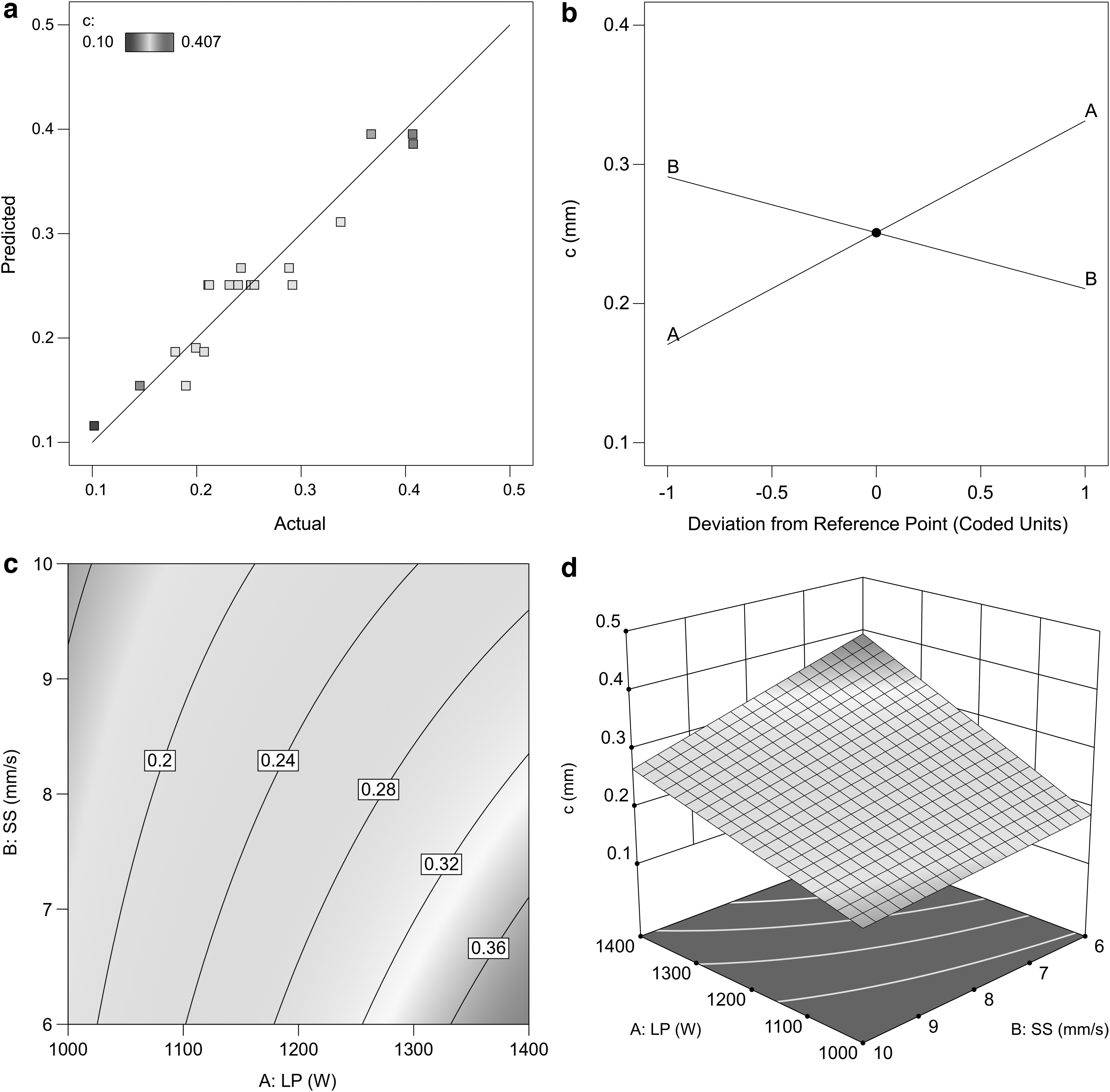
Model-related statistics graphs for c. (a) Predicted versus actual; (b) perturbation; (c) contour line of c w.r.t AB; (d) 3D response surface of c to AB.

Figure 25c and d shows the interaction effects of laser power and scanning speed on the heat source depth. It can be observed that as scanning speed increases, the partial derivative of heat source depth to laser power is getting smaller. This is veriied by the derivatives of c to the factors, as calculated in Equation (14). This may be explained by the thermal capacity of substrate. Higher scanning speed reduces the specific energy into the material, thereby penetration of laser beam is gradually increased by laser power. On the contrary, small increment of laser power would be sensitively represented by increase of penetration.

Coefficient realizability analysis

Figure 26 plots the overlay area of three factor pairs with target responses settled as η > 0.65, r ∈[1.4, 1.6], and c ∈[0.19, 0.25]. The range of target responses are typically assigned from the distribution of calibrated values, that is, [0.6, 0.8], [1.1, 2.0], and [0.1, 0.4], respectively. Both the targets are around the center points of proposed design matrix with about 20% margin of the entire range.

FIG. 26.

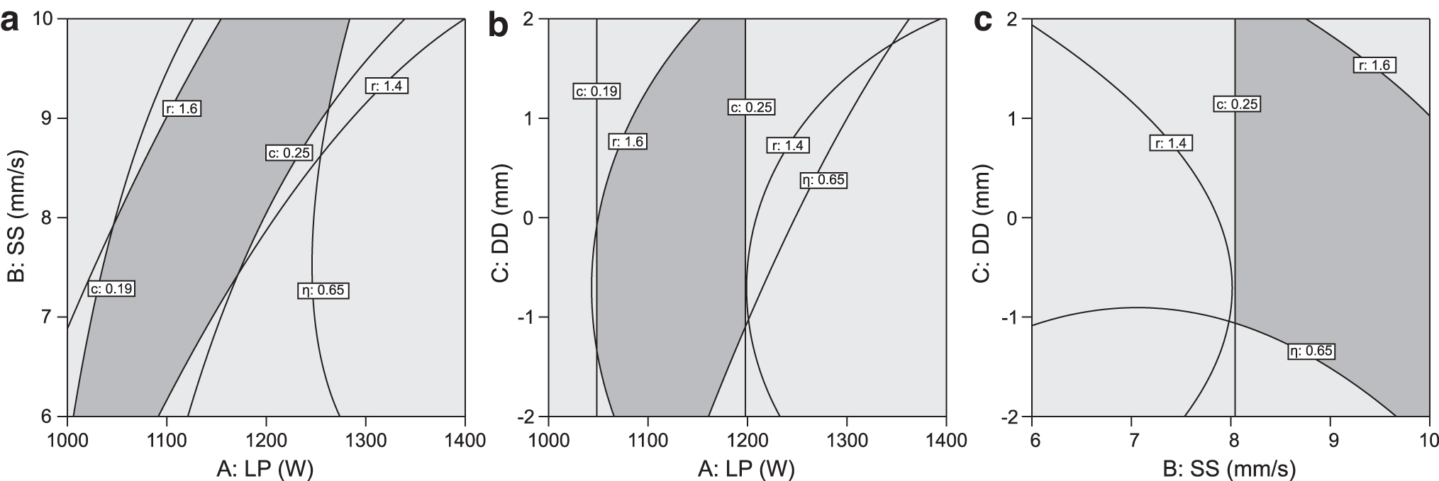
Overlay plot with target heat source coefficients. (a) DD = 0; (b) SS = 8; (c) LP = 1200.

The shadow area in yellow signifies the parameter space fulfilling the target. As can be seen from Figure 26a, the optimal parameter space is a stripe inclined toward the bottom left corner. When considering the interaction of AC (laser power x defocusing distance) and BC (scanning speed x defocusing distance), as shown in Figure 26b and c, the optimal parameter space moves toward the right side with greater areas. Specifically, at D_f = 0 mm, the linear energy input ranges from about 121.8 to 174.7 J·mm⁻¹.

At v = 8 mm·s⁻¹, the optimal space for laser power is from 1050 to 1200 W. The optimal space for scanning speed is >8 mm·s⁻¹ when p = 1200 W. Therefore, appropriate heat source coefficients can be identified by selecting laser process parameters at ∼1100 W of laser power, 9 mm·s⁻¹ of scanning speed, and −0.5 mm of defocusing distance.

Validation of Heat Process Models

According to the simulation model established in Heat Process Correlations section, heat source parameters were inversely resolved for all the laser surfacing process conditions. The correlation between heat source coefficients and laser surfacing parameters was thus established. It is still necessary to check the feasibility of built heat process models. Validation of the relationship was conducted by comparing bead geometries of four process conditions. The reasons are that these parameter settings are typical representations within the design domain.

Conditions 2 and 13 are around the center of parameter settings, embodying commonly applied conditions. Conditions 17 and 20 represent the extreme situation when the maximum and minimum energy density is input into the substrate. Such a selection would be capable of validating the generalization of established heat process models. Processing parameters and corresponding heat source coefficients, as calculated by substituting the variable values into Equations (9), (11), and (13), are illustrated in Table 14.

Table 14.

Process Parameters Used for Validation Tests

Run	P, W	v, mm·s⁻¹	D_f, mm	η	r, mm	c, mm
2	1400	6	2	0.660	1.257	0.395
13	1200	8	0	0.663	1.409	0.251
17	1200	5	0	0.677	1.242	0.338
20	1200	8	−3	0.633	1.491	0.255

With the coefficients, heat transfer analysis of laser surfacing was carried out to obtain the temperature distribution and thus bead geometry. Figure 27 compares the melt pools of experimental specimens with finite element results. Owing to geometric symmetry, the whole cross-sectional images are halved and combined into one for convenient comparison. Detailed data of the validation are illustrated in Table 15.

FIG. 27.

Comparison between experimental and numerical melt pool geometry. (a) Second test sample; (b) 13th test sample; (c) 17th test sample; (d) 20th test sample.

Table 15.

Comparison of Simulated Bead Geometry to Experimental Counterparts

Run	Item	Width, mm	Depth, mm	Area, mm²
2	Experiment	2.886	1.149	2.375
	Simulation	2.804	1.150	2.464
	Relative error	2.84%	0.08%	3.75%
13	Experiment	2.562	0.886	1.603
	Simulation	2.541	0.876	1.662
	Relative error	0.80%	1.15%	3.68%
17	Experiment	2.762	1.067	2.093
	Simulation	2.608	1.003	1.988
	Relative error	5.58%	6.00%	5.20%
20	Experiment	2.438	0.826	1.369
	Simulation	2.373	0.738	1.334
	Relative error	2.68%	10.68%	2.56%

From the figure and table, one can find that the prediction errors for extreme conditions are slightly higher than normal ones. But only the prediction of depth is >6%. Apart from that, the relative errors are <3.75% for most commonly used parameter settings. Therefore, the validation demonstrates good accuracy of established heat process correlations.

Methodology Versatility

The methodology proposed in this study is validated to be feasible for revealing the effects of additive manufacturing process parameters on heat source coefficients. However, there are still some aspects needed to be further investigated to assure general applicability, including data availability, process extendability, and material coverage.

Data availability

The correlation method presented is based on RSM. Therefore, a certain number of experimental and numerical data should be available for implementation. According to RSM, the necessary data amount is determined by the number of interested process parameters. Although taking more influencing factors into consideration would mean a better understanding about the relationships, large amount of data set and nonlinearity effects would prohibit the methodology from successful implementation.

Process extendability

Generally, the methodology is extendable for powder bed-based additive manufacturing technologies, such as selective laser melting and electron beam melting, because of similar boundary conditions.

The ease of extension may be quite different, owing to the diversity of process couplings. Application to the processes such as direct energy deposition and other wire-based additive manufacturing technologies will need to address the effects of accumulated geometry on heat source. New difficulties may be encountered when implemented to wire and arc additive manufacturing, which involves much more process parameters and stronger coupling effects.

Material coverage

The methodology proposed in this research should be applicable to any material providing that the properties are available. However, some temperature-dependent material properties may not be easily obtained, which would render great divergence between experimental and numerical results. Furthermore, the nonlinearity of material properties would also influence the methodology application. The greater degree of nonlinearity, the more difficulty of establishing the relationships. But once successfully identified, huger advantages would be benefited from application of the proposed methodology.

Conclusions

An inverse solution approach based on RSM was applied to study the effects of laser-based additive manufacturing process on heat source model coefficients. Experimental study was first conducted to investigate the influences of process parameters on bead geometry characteristics. Then, numerical thermal analysis of laser surfacing was carried out to reveal the effects of heat source model coefficients on bead geometry. With experimental targets, heat source model coefficients corresponding to processing conditions were inversely identified for heat process correlation. From the results acquired, the following conclusions can be drawn:

Experimentally obtained bead geometry is approximately linear with laser power and scanning speed, but parabolically determined by defocusing distance. Increase in laser power, and/or decrease in scanning speed, lead to increase of bead geometry characteristics.

Numerically calculated bead geometry is determined by three heat source coefficients and scanning speed in quadratic manner. The bead geometry is positively relevant with specific heat input.

The proposed methodology is capable of correlating heat source coefficients to process parameters with good accuracy and efficient computation cost. Three heat model coefficients are quadratically dependent on the process parameters.

Footnotes

Acknowledgment

The authors are thankful for the support from Public Service Platform for Technical Innovation of Machine Tool Industry in Fujian Province.

Authors' Contributions

Conceptualization, methodology, supervision, and writing—reviewing and editing by C.C. Investigation, formal analysis, software, and writing—original draft by J.Z. Validation and visualization by T.Z. Project administration, writing—reviewing and editing by G.L. Writing—reviewing and editing by X.H.

Author Disclosure Statement

The authors declare that they have no known competing financial interests or personal relationships that could have appeared to influence the study reported in this article.

Funding Information

This study was financially supported by the Natural Science Foundation of Fujian Province, China (Grant No. 2020J01873), Science & Technology Major Project of Fujian Province, China (Grant No. 2020HZ03018), and Start-up Foundation of Fujian University of Technology (Grant No. E0600276).

References

Fan

, Zhang

. Study on process optimization of WC-Co50 cermet composite coating by laser cladding. Int J Refract Met Hard Mater, 2020; 87:105133.

Yusof

MFM

, Ishak

, Ghazali

. Classification of weld penetration condition through synchrosqueezed-wavelet analysis of sound signal acquired from pulse mode laser welding process. J Mater Process Technol, 2020; 279:116559.

Biswas

, Mandal

, Vasu

, et al. Analysis of welding distortion due to narrow-gap welding of upper port plug. Fusion Eng Des, 2010; 85(5):780–788.

Liu

, Zhu

, Peng

, et al. Microstructure prediction of selective laser melting AlSi10mg using finite element analysis. Mater Des, 2018; 142:319–328.

Liu

, Zhang

, Xue

. Numerical investigation on residual stress distribution and evolution during multipass narrow gap welding of thick-walled stainless steel pipes. Fusion Eng Des, 2011; 86(4–5):288–295.

Chen

, Lin

, Ou

, et al. Study of heat source calibration and modelling for laser welding process. Int J Precis Eng Manuf, 2018; 19(8):1239–1244.

Rosenthal

. The theory of moving sources of heat and its application to metal treatments. Tans ASME, 1946; 68:849–866.

Manca

, Morrone

, Naso

. Quasi-steady-state three-dimensional temperature distribution induced by a moving circular Gaussian heat source in a finite depth solid. Int J Heat Mass Transf, 1995; 38(7):1305–1315.

Zubair

, Chaudhry

. A unified approach to closed-form solutions of moving heat-source problems. Heat Mass Transf, 1998; 33(5):415–424.

10.

Nguyen

, Mai

, Simpson

, et al. Analytical approximate solution for double ellipsoidal heat source in finite thick plate. Weld J, 2004; 83:82.

11.

Araya

, Gutierrez

. Analytical solution for a transient, three-dimensional temperature distribution due to a moving laser beam. Int J Heat Mass Transf, 2006; 49(21–22):4124–4131.

12.

Myhr

, Grong. Dimensionless maps for heat low analyses in fusion welding. Acta Metallurgica, 1990; 38(3):449–460.

13.

Azar

, Ås

, Akselsen

. Determination of welding heat source parameters from actual bead shape. Comput Mater Sci, 2012; 54:176–182.

14.

, Gao

, Zhang

, et al. Analytic weld pool model calibrated by measurements part 1: Principles. Weld J, 2017; 96(6):193s–202s.

15.

, Gao

, Zhang

, et al. Measurement of calibrated recursive analyticin the gas tungsten arc weld pool model. Weld J, 2018; 97(4):108s–9s.

16.

, Gu

, Lourenco

, et al. Parameter determination of double-ellipsoidal heat source model and its application in the multi-pass welding process. Ships Offshore Struct, 2015; 10(2):204–217.

17.

Goldak

, Chakravarti

, Bibby

. A new finite element model for welding heat sources. Metall Trans B, 1984; 15(2):299–305.

18.

Ning

, Sievers

, Garmestani

, et al. Analytical modeling of transient temperature in powder feed metal additive manufacturing during heating and cooling stages. Appl Phys A, 2019; 125(8):707.

19.

Ning

, Sievers

, Garmestani

, et al. Analytical modeling of in-process temperature in powder feed metal additive manufacturing considering heat transfer boundary condition. Int J Precis Eng Manuf Green Technol, 2020; 7(3 Suppl):585–593.

20.

Walker

, Bennett

. An automated inverse method to calibrate thermal finite element models for numerical welding applications. J Manuf Process, 2019; 47:263–283.

21.

Kim

, Lee

, Cho

. Analysis of pulsed Nd:YAG laser welding of AISI 304 steel. J Mech Sci Technol, 2010; 24(11):2253–2259.

22.

Belitzki

, Marder

, Huissel

, et al. Automated heat source calibration for the numerical simulation of laser beam welded components. Prod Eng, 2016; 10(2):129–136.

23.

Majumdar

, Xia

. A Green's function model for the analysis of laser heating of materials. Appl Math Model, 2007; 31(6):1186–1200.

24.

Kidawa-Kukla

. Temperature distribution in a rectangular plate heated by a moving heat source. Int J Heat Mass Transf, 2008; 51(3–4):865–872.

25.

Veldman

DWM

, Fey

RHB

, Zwart

, et al. Semi-analytic approximation of the temperature field resulting from moving heat loads. Int J Heat Mass Transf, 2018; 122:128–137.

26.

Cole

, Cetin

, Demirel

. Semi-analytical source method for reaction–diffusion problems. J Heat Transf, 2018; 140(6):0161301.

27.

Çetin

, Kuṣcu

, Çetin

, et al. Semi-analytical source (SAS) method for 3-D transient heat conduction problems with moving heat source of arbitrary shape. Int J Heat Mass Transf, 2021; 165:120692.

28.

Box

GEP

, Wilson

. On the experimental attainment of optimum conditions. J Royal Stat Soc, 1951; Series B, 13:1–45.

29.

Chelladurai

SJS

, K M, Ray

, et al. Optimization of process parameters using response surface methodology: A review. Mater Today Proc, 2021; 37:1301–1304.

30.

Torabi

SHR

, Alibabaei

, Bonab

, et al. Design and optimization of turbine blade preform forging using RSM and NSGA II. J Intell Manuf, 2017; 28(6):1409–1419.

31.

Denlinger

, Jagdale

, Srinivasan

, et al. Thermal modeling of Inconel 718 processed with powder bed fusion and experimental validation using in situ measurements. Addit Manuf, 2016; 11:7–15.

32.

Luo

, Zhao

. A survey of finite element analysis of temperature and thermal stress fields in powder bed fusion additive manufacturing. Addit Manuf, 2018; 21:318–332.

33.

Rong

, Mi

, Xu

, et al. Laser penetration welding of ship steel EH36: A new heat source and application to predict residual stress considering Martensite phase transformation. Mar Struct, 2018; 61:256–267.

34.

Pang

, Liu

, Zhang

, et al. Simulation research on the thermal-mechanical coupling of YSZ thermal protective coatings prepared by laser-plasma composite heat source on the surface of high-intensity diesel engine cylinder head. Optik, 2020; 207:164425.

35.

Amine

, Newkirk

, Liou

. Investigation of effect of process parameters on multilayer builds by direct metal deposition. Appl Therm Eng, 2014; 73(1):500–511.

36.

Zhou

, Wang

, Choi

, et al. Robust optimization for reducing welding-induced angular distortion in fiber laser keyhole welding under process parameter uncertainty. Appl Therm Eng, 2018; 129:893–906.

37.

Sun

, Shi

, Pei

, et al. Heat transfer and temperature distribution during high-frequency induction cladding of 45 steel plate. Appl Therm Eng, 2018; 139:1–10.

38.

Liu

, Fan

, Yin

, et al. Effect of caliber rolling reduction ratios on the microstructure and mechanical properties of 45 medium carbon steel. Mater Sci Eng A, 2020; 774:138954.

39.

Zhao

, Zhang

, Liu

, et al. influence mechanism of laser defocusing amount on surface texture indirect metal deposition. J Mater Process Technol, 2023; 312:117822.