Dual-Robot Nonplanar 3D Printing Path Planning and Compensation

Abstract

The traditional planar layered printing process struggles to accommodate such complex geometries, while nonplanar layering printing offers promise. Yet, nonplanar layering printing encounters two key challenges: One is that nonplanar paths often cause extremely uneven interlayer path spacing; The other is that printing with large overhangs creates many difficulties. Therefore, this article proposes methods involving path compensation and a high degree-of-freedom dual-robot system to address these issues, which has more advantages when printing single-shell surfaces with high curvatures, overhangs, or branches. The proposed method operates in several stages: First, it derives the initial printing path and compensates for the path at sparse positions. Second, this method introduces a dynamic-based method to homogenize and optimize the compensated path. Finally, the study presents the derivation of the two robots’ poses based on the printing path and conducts printing experiments. Additionally, the study compares and analyzes the compensation and homogenization results by different methods, validating their effectiveness.

Keywords

dual-robot nonplanar printing path compensation dynamic relaxation path homogenization turntable

Introduction

3D printing is a process of accumulating materials in space, represented by fused deposition modeling (FDM).¹ Currently, the most common 3D print path planning method is planar layering, where a list of parallel planes slices the geometry, creating a layer-by-layer upward printing path. However, planar layered printing has great difficulties when printing geometries with high curvatures or overhangs, while nonplanar layering shows potential. Nonplanar printing, also called curved layers printing, layers geometries in a nonplanar manner to form the printing paths, developed with the introduction of the high degrees-of-freedom (DOF) robot.

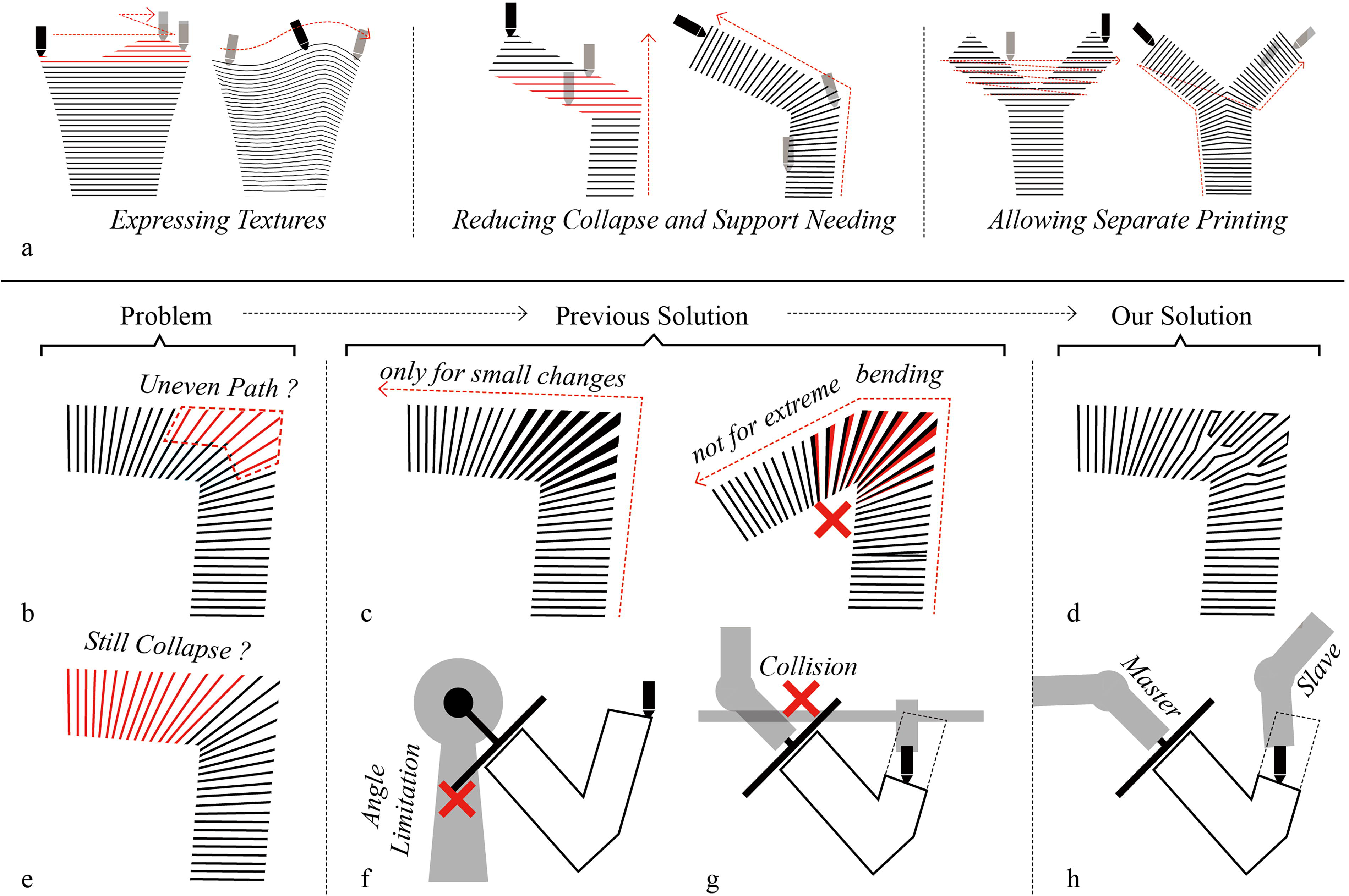
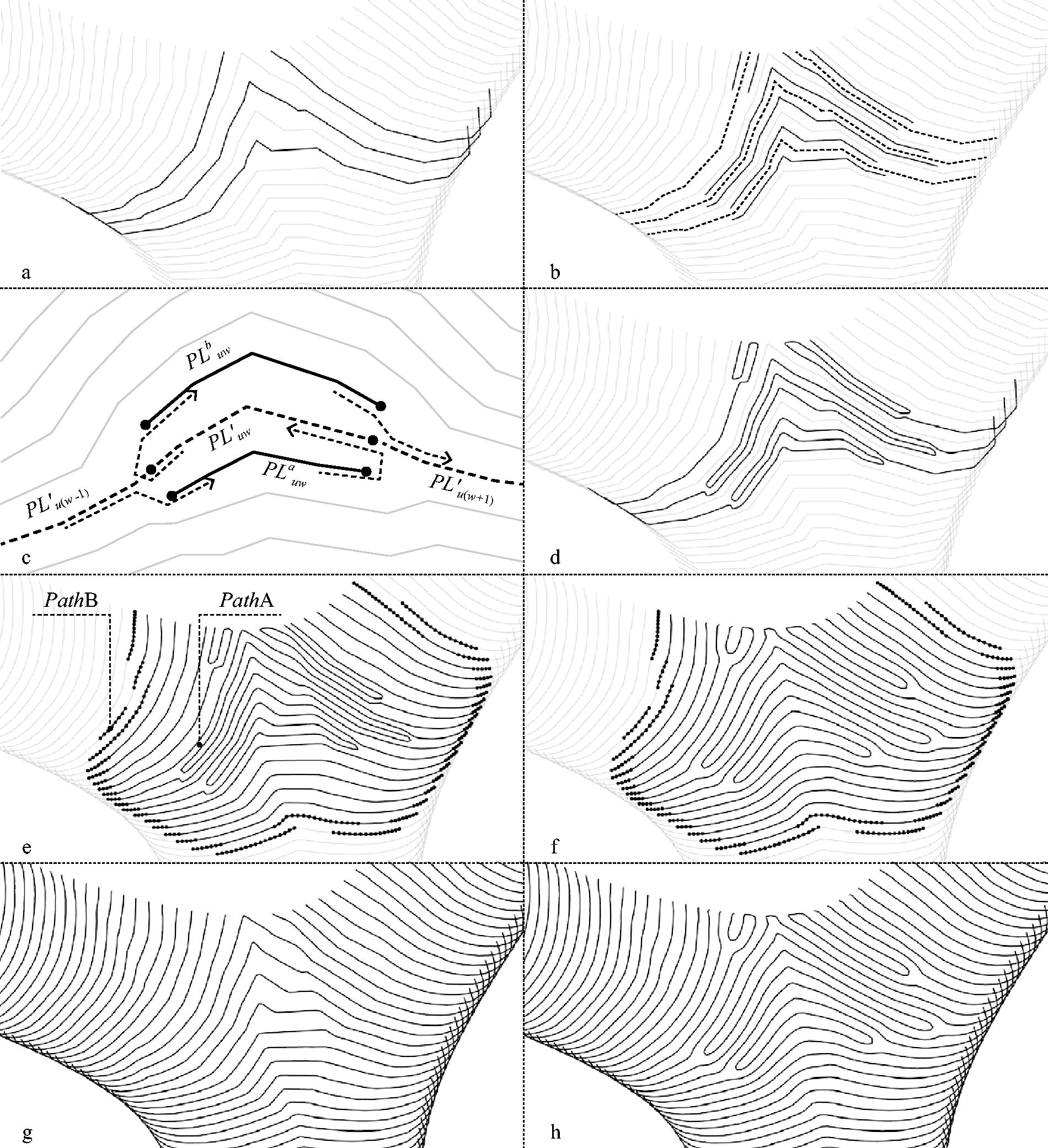
Nonplanar printing offers several advantages over planar printing (Fig. 2A): It reduces the need for supporting structures to save materials and time, facilitates separate printing of branches to ensure material extrusion continuity, enhances mechanical properties by adjusting the filament printing path and the mechanical anisotropy (Guidetti et al.² formed nonplanar paths by stress flow of the object to increase its mechanical properties), improves texture expression. However, current nonplanar printing methods still face limitations when printing geometries with high curvatures or overhangs:

Nonplanar printing inevitably leads to uneven layer spacing paths (Fig. 2B). Regarding this, Xu et al.³ parametrically calculated the robot tool speed to control the extrusion volume of the material and match the interlayer spacing. However, their methods are limited to small interlayer spacing changes, making them unsuitable for highly curved layers (Fig. 2C). Additionally, offline printing also complicates the control of printhead extrusion. Knöppel et al.⁴ proposed a method generating uniform stripe based on the convex-quadratic energy. However, the methods based on this inspiration cannot quickly sort the paths and cause many path interruptions. So, this article proposes a method to compensate paths around sparse paths (Fig. 2D) and homogenize paths to optimize them.

Dealing with geometries with significant tiltings and hangings, printing on the fixed platform will lead to collapse (Fig. 2E). Wang et al.⁵ used a 5-DOF printing system with a turntable. Coupek et al.⁶ used a printing system with a cylindrical body to be printed on. However, their DOF and tilt ranges are still limited (Fig. 2F). Wu et al.⁷ and Keating et al.⁸ both proposed a system with a fixed extruder and a 6-DOF robot driving a turntable. However, such systems also have spatial limitations (Fig. 2G). This article proposes a system with two 6-DOF robots driving a turntable and a printhead, providing multiple print angles while ensuring space flexibility (Fig. 2H).

In summary, this method is primarily for printing single-shell surfaces with high curvatures or overhangs, which could not be printed continuously without support in previous studies due to limits in the device and uneven path layer spacing. The innovations and addressed problems in this article include: a.

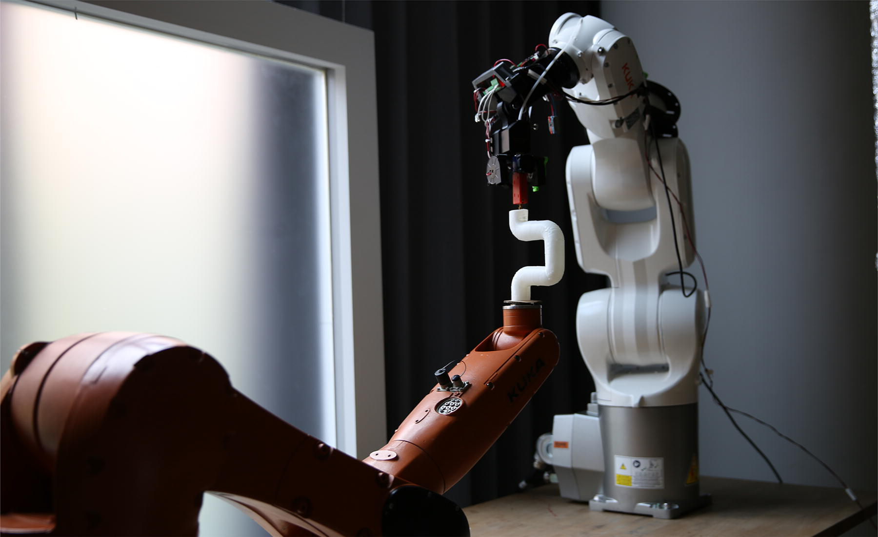
Proposes a continuous path compensation method for nonplanar printing based on distance field and dynamic relaxation in the “Path Compensation Method” section, addressing the issues of uneven paths.

Analyzes the layer spacing uniformity before and after compensation and homogenization in the “Path Compensation Discussion” section, proving the effect of printing path compensation.

Proposes a 6-DOF dual-robot system and completes printing experiment (Fig. 1) in the “Dual-Robot Derivation and Printing Experiment” section, addressing the issues of high tilt printing or overhang printing.

FIG. 1.

Dual-robot nonplanar 3D printing path planning and compensation.

FIG. 2.

Introduction.

Path Compensation Method

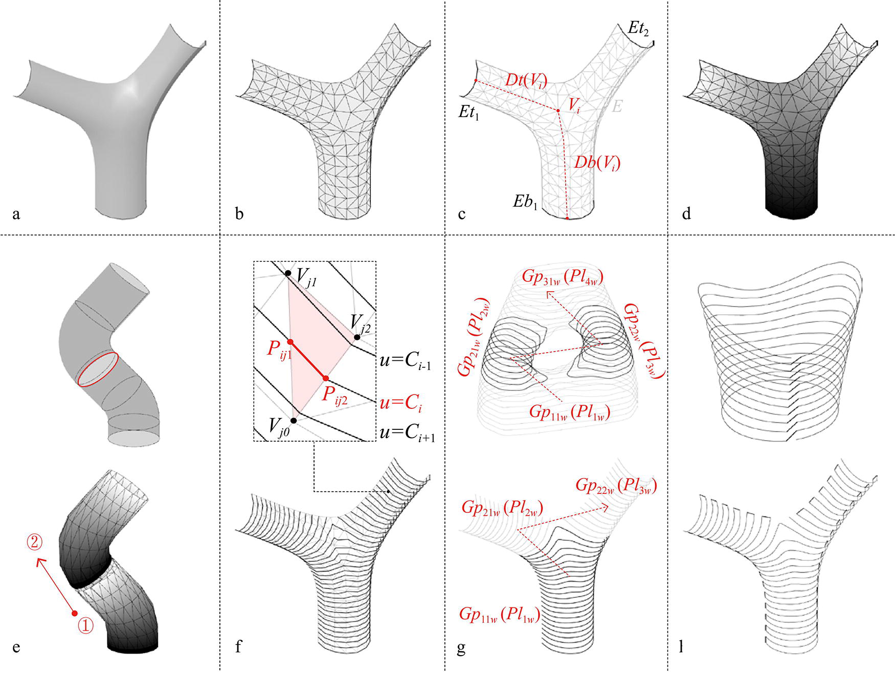
This article limits the input geometry to single-shell surfaces with upper and lower edges determined, taking the geometry shown in Figure 3A as an example at about 50 mm height. Furthermore, programs of this method run in a Grasshopper environment, which is software for parametric modeling, program writing, or graphics computation.

FIG. 3.

Initial paths generation.

Preprocessing: Distance field and initial paths

Generally, researchers always plan nonplanar paths based on field models. Mitropoulou et al.⁹ generated a scalar distance field on the geometry based on the geodesic distance and extracted nonplanar printing paths according to the isopleths of the field. Kout et al.¹⁰ generated contour-parallel isopleths by additively weighted distance functions. Dai et al.¹¹ proposed a multiaxis motion 3D printing method for freeform volume by accumulation field, enabling unsupported printing on curved layers. Shan et al.¹² formed nonplanar printing paths based on isothermal surfaces of a heat conduction model. Li et al.¹³ proposed two orthogonal unit vector fields to optimize paths and printing orientations. This section adopts the method used by Mitropoulou et al., writing a similar program to extract the Initial Paths by Grasshopper components.

Input and conversion

Firstly, the geometry in NURBS (Non-Uniform Rational B-Splines) or Mesh format is input and converted into a triangular mesh with appropriate triangular density (Fig. 3B) by Quad Remesh, a component in Grasshopper, to approximate the input model for calculation. Higher density improves path accuracy but increases computing time.

Distance field generation

For practical calculations, this method only calculates the distance field values of the mesh vertices, and the geodesics distance, defined by the shortest curve via mesh between two points, is used based on the previous study¹⁴ and rewritten in the environment. Specifically, this method finds all mesh vertexes as V_i (i = 0,., n) and the bottom and top naked edges Eb_n and Et_m (format of polyline list) as the beginning and ending during printing, respectively. Then, this method finds the shortest geodesic distance from V_i to the Eb_n and Et_m via the mesh, as Db(V_i) and Dt(V_i) (Fig. 3C). The geodesic from a point to a curve can be approximated by the shortest one among all the geodesics from that point to multiple equidistant points on the curve. Based on the above, the distance field satisfies (1).

u (V_{i}) = \frac{{D b (V_{i})}^{α}}{{D b (V_{i})}^{α} + {D t (V_{i})}^{α}}, (α = \frac{\sqrt{5} - 1}{2}, i = 0, . . ., n) .

(1)

This function ensures that the range of u uniformly distributes in [1,0] and values near Eb_n and Et_m are close to 0 and 1, respectively. For image display, the scalar value u(V_i) of V_i forms a visual color scalar graph of the distance field on the mesh (Fig. 3D). In addition, a complex geometry can be split and calculated separately (Fig. 3E).

Isopleth generation based on interpolation

In this distance field, this method extracts its isopleths by (2).

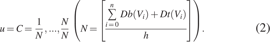
u = C = \frac{1}{N}, . . ., \frac{N}{N} (N = [\frac{\sum_{i = 0}^{n} D b (V_{i}) + D t (V_{i})}{h}]) .

(2)

Where N is the number of layers determined based on the average unfolded length of the mesh, h = 1.2 mm is the input layer spacing (according to the printhead diameter), and “[ ]” is the rounding function.

Furthermore, we use a linear interpolation method to form the isopleths u = C. Specifically, for the triangle face Face_j (j = 0,., m, m is the number of faces) in the mesh, let its three vertices be V_j₀, V_j₁, V_j₂ (u(V_j₀)≤u(V_j₁)≤u(V_j₂)). If there is C _i (i = 0,., N) and {x, y}={0,1},{0,2},{1,2}, such that u(V_jx)≤C _i ≤u(V_jy), then this method obtains the interpolation point, satisfying (3).

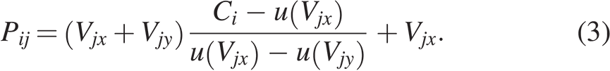
P_{i j} = (V_{j x} + V_{j y}) \frac{C_{i} - u (V_{j x})}{u (V_{j x}) - u (V_{j y})} + V_{j x} .

(3)

For the given j and i, if the P_ij list contains two different points, they can be concatenated as a line. All lines are combined to form Path_i, as shown in Figure 3F.

Sorting and seaming

Sorting

Sorting paths solely by isopleth value when printing multibranch objects would cause the printhead to frequently move between branches, which is time-consuming and may lead to material stringing between branches. We should ensure that the printhead completes one branch before moving to the next, ensuring printing continuity, time-saving, and quality. First, we sort the polylines in Path_i layer by layer according to the order of the ones in the previous layer (based on the polyline geometric center). Second, we divide the Path_i into groups Gp_n according to the polyline list length in each layer. Third, we transpose the multidimensional array Gp_nwv to form a new sorting as Gp_nvw. Finally, we combine the array Gp_nvw to form polyline lists Pl_uw (Fig. 3G).

Seaming

We use an algorithm to adjust the starting points and directions of paths by their previous paths, ensuring zig-zag upward paths for open isopleths and spiral upward paths for closed isopleths as Figure 3H.

Path compensation by distance field

In this section, we compensate for paths in the sparse part of the Initial Path and consider a reasonable connection between the compensated paths and the Initial Path, ensuring continuous and reasonable printing. Specifically, we still generate compensation paths by the distance field and trim them, which method is more stable with greater logical consistency than tweening between layers. For the input Initial Path (polyline format), the specific steps are as follows:

Sparse layers selecting

For less computation, calculations are performed only on layers with sparse regions. First, for all layers of paths Path_i+₁ (i = 0,., N − 1, N is the number of layers), this method defines D_i (i > 0) as the maximum distance from all the points on Path_i₊₁ to the curve of Path_i₋₁, approximated by the maximum distance between the curve and the d-equidistant vertices (d = 1.2 mm in this method) of the other curve. (The d-equidistant is the equal walking length segments on the curve with the accuracy d, approximated by n divided equal length segments, where n = [l/d], l is the curve length, and “[ ]” is the rounding function.) Second, we define retention parameters r = A/B to delete some compensated paths intermittently. Specifically, for all Path_i, this method selects its subset as Path_i’ (i′>0) (Fig. 4A) satisfying:

D_{i'} > a h, i' mod B < A

(4)

Where a = 1.4 is the proportional parameter, h = 1.2 mm is the layer spacing mentioned earlier, and r = A/B = 1/2.

FIG. 4.

Path compensation and path homogenization.

Compensation path forming and trimming

For the selected paths, we extract the two compensation path isopleths Path^a_i′ and Path^b_i′ between Path_i’ and Path_i′−1, Path_i′+₁, respectively. Specifically, the equation of the isopleth is:

u = C = \frac{1}{N} (i' \pm \frac{1}{2}) .

(5)

In addition, if the number of the curves of Path^a_i′ and Path^b_i′ is different, it is deleted.

Then, this method d-equidistant segments Path^a_i′ and Path^b_i (d = 1.2 mm), corresponding them one-to-one to form small segments called l^a_i′j and l^b_i′j. This method selects j′ in l^a_i′j′ and l^b_i′j′, which satisfies (6).

D_{i' j'} > a h .

(6)

Where D_i′j′ is the distance between the midpoint of l^a_i′j′ and l^b_i′j′. Combine the remaining paths to form double-layer circuit paths Path^a_i′z and Path^b_i′z (Fig. 4B).

Compensation path connecting

We reorder the compensated paths Path^a_i′z and Path^b_i′z into PL^a_uv and PL^b_uv, following the sorting process in the "Sorting and seaming" section. In addition, this method breaks paths PL_u based on PL^a_uv and PL^b_uv and weaves them in the principle of bottom-up, inside-out. Specifically, paths PL_u are broken at the nearest points to the endpoints of PL^b_uv to form PL′_uw (w = 0,2,., v), combining with the compensation path to form (7).

P L_{u} = {P L {'_{u}}_{0}, {P L^{b}}_{u}_{1}, P L {'_{u}}_{1}, {P L^{a}}_{u}_{1}, P L {'_{u}}_{2}, {P L^{b}}_{u}_{2},...}

(7)

So, all elements in PL_u are connected end-to-end by the seaming method in the “Sorting and Seaming” section (Fig. 4C), forming the compensation path (Fig. 4D).

Path homogenization by dynamic relaxation

This section is an additional optimization step to alleviate situations where some compensated paths are too dense. The inspiration for this method comes from the simple growth simulation process shown in the previous study,¹⁵ which homogenized and tilled curves by endowing their mechanical properties. Specifically, this method uses the dynamic relaxation algorithm to homogenize the paths by endowing the geometry with some physical properties to simulate its growths and shape changes. The homogenizing details of the polyline paths are as follows:

Simulation tools and method

For calculations, we use the Kangaroo developed by Daniel Piker,¹⁶ a parametric designing plug-in in Grasshopper, to simulate physics like springs or gravity for diverse parametric designing of complex forms and structures. We use Kangaroo to simulate the temporal variation of the shape by endowing it with physical properties.

Calculation range

For less computation, only compensated paths and nearby path segments are calculated. Specifically, this method defines the minimum distance from each path segment to compensated paths (Path^a_i′z or Path^b_i′z) as d, selecting path segments that satisfy d<r₁ as PathA, and r₁<d<r₂ as PathB, shown in Figure 4E.

Imparting physical properties

This method gives some physical properties to the input path for further calculation:

Keep PathB and its nodes fixed.

Keep the nodes of PathA on the geometry.

Give the polylines and vertices of PathA and PathB the property of Collider, which is a physical model simulating polylines as strips with the radius h, positively correlating with the layer spacing.

Give the angular elasticity of each node of PathA with the force of F.

Give the length elasticity of each segment of PathA with the elastic range of R and the force of F′.

Simulating and results

Based on the above, the paths are homogenized (Fig. 4F). The Initial Path and the compensation and homogenization result are shown in Figure 4G, H.

Path Compensation Discussion

Method B: Compensating paths under layers

Unlike the compensating method in the “Path Compensation by Distance Field” section (Method A), this article also considers another method of compensating all paths below sparse paths (Method B), which compensates double-layer paths below the Initial Path and forms a reciprocating loop path, ensuring the continuous and uninterrupted paths. Then, this method sets the retention parameter r = A/B = 2/3 to reduce the compensation paths appropriately. Similar to the “Path Homogenization by Dynamic Relaxation” section, this method utilizes dynamic relaxation to homogenize the paths, as Figure 5C.

FIG. 5.

Analyzing of homogenization effects.

Analysis of interlayer spacing

This article extracts and analyzes a segment of the paths with the compensated paths to demonstrate the effectiveness of Path Compensation and Path Compensation.

The analysis method calculates the distance D between each d-equidistant vertice point (d = 1.2 mm) in the paths to the printed paths below. Then, we obtain the distribution frequency of all D within a list of equally spaced intervals. Uniform paths lead to a concentrated distribution. For this analysis method, we analyze the compensation and homogenization results under Method A (r = 1/2) (Fig. 5B) and Method B (r = 1 or 2/3) (Fig. 5C).

According to the analysis, Path Compensation significantly reduces the parts with large interlayer spacing, but it makes some smaller interlayer spacing, which can be relieved after homogenization. Methods A and B (r = 2/3) can ensure the compensation and homogenization effect, but Method A takes less time during homogenization, even needless homogenization.

Dual-Robot Derivation and Printing Experiment

Dual-robot printing system setup

This method uses a system with two robots to nonplanar print. The system mainly includes a Robot A with the printhead and a Robot B with the turntable shown in Figure 6A. Specifically, each component is as follows:

FIG. 6.

Dual-robot system setup and PrintHead relative orientation.

A. Robot A. KUKA KR6 R700 Robot, a 6-axis industrial robot driving the 3D printhead.

B. PrintHead. A plastic extruder component for 3D printing for melting and extruding the plastic filament (Polylacticacid (PLA) fiber in this article) during printing.

C. Robot B. KUKA Agilus KR6-10 R900 Robot, another 6-axis robot driving the turntable.

D. Turntable. A platform with 20 cm diameter supporting 3D printing on the end of the Robot B.

Motion derivation and printing

To get the motion codes of two robots by the printing paths, we first calculate the relative orientation plane list (relative-Pln) for the printhead moves relative to the turntable plane over time and then derive the absolute motion orientation plane lists of the two robots with turntable and printhead in world coordinates, named as turntable-Pln and printhead-Pln (Fig. 6A). Next, we derive the plane list into robot motion code by KUKA-PRC,¹⁷ a Grasshopper plug-in integrating with KUKA robot systems to allow users to plan robot paths.

Reachability of robot arm

Considering the normal vectors of printhead-Pln should be nearly vertical downward, turntable-Pln may become complex. Therefore, it is necessary to study the robot’s reachability to determine the initial position of the printed geometry and the turntable quickly and reasonably.

Specifically, we generate the reachability of the robotic arm to a point in one orientation by inverse kinematics and write this judging program by KUKA-PRC in Grasshopper. We analyze the reachability of Robot B in multiple orientations at each point in the spatial array and display the reachability map as the heatmap shown in Figure 6B. In this map, we limit the positions of the turntable-Pln to some points whose reachable orientations can approximately cover the normal vectors of the turntable-Pln shown in Figure 6C.

However, the robot’s reachability at one point does not necessarily imply that it can reach that point directly from any previous position, and the discrete mapping may be inaccurate. So, this position determination is just a rough method needing further adjustment in the experiment.

PrintHead relative orientation generation

This method involves extracting the normals of the relative-Pln by the geometry’s normal vectors and the tangent vectors of the Initial Path. For one point on the path, we extract the tangent vector (t) of the corresponding Initial Path on its nearest point and the normal vector (n) of the input geometry on its closest point, resulting in the vector z = t × n. The normalized z should be collinear with the z-axis of the relative-Pln. Since the printed geometry may be highly curved, it is not correct to keep all z upwards. So, whether to flip z is determined by the position relationship between this point and the previous layer’s path, ensuring the backs of the relative-Pln face the latter. Furthermore, the “Robot Pose Derivation and Printing Experiment” section will adjust the x-axis of the relative-Pln by the robots’ positions in the future for a convenient pose for the robot (Fig. 6D).

This printing method will face situations such as saddle surfaces causing singularities. Near it, the relative-Pln may suddenly change or collide with printed objects. So, considering this, this method adjusts z as z′ shown in Figure 6E, F, satisfying:

z^{'} = z + t (z_{a v e} - z), t = t_{0} (n \cdot z_{a v e})

(8)

The z _ave is the normalized average of all z of the d-equidistant vertice points (d = 1.2 mm) on the path. When the point approaches singularities, the angle between n and z _ave will become very small, t will approach t₀, and z′ will approach z _ave if t₀ = 1 (t₀ = 0.75 in this method). When away from singularities, t will approach 0, and z′ will approach z.

Robot pose derivation and printing experiment

This section derives relative-Pln to turntable-Pln and printhead-Pln and simulates robots plane-by-plane in KUKA-PRC by RoboTeam,¹⁸ which is a software toolkit to coordinate and control multiple KUKA robots for efficient collaboration and cooperative production in complex tasks. Facing different types of geometries, we propose different derivation methods and complete the printing experiment.

Method of Turntable Fixed

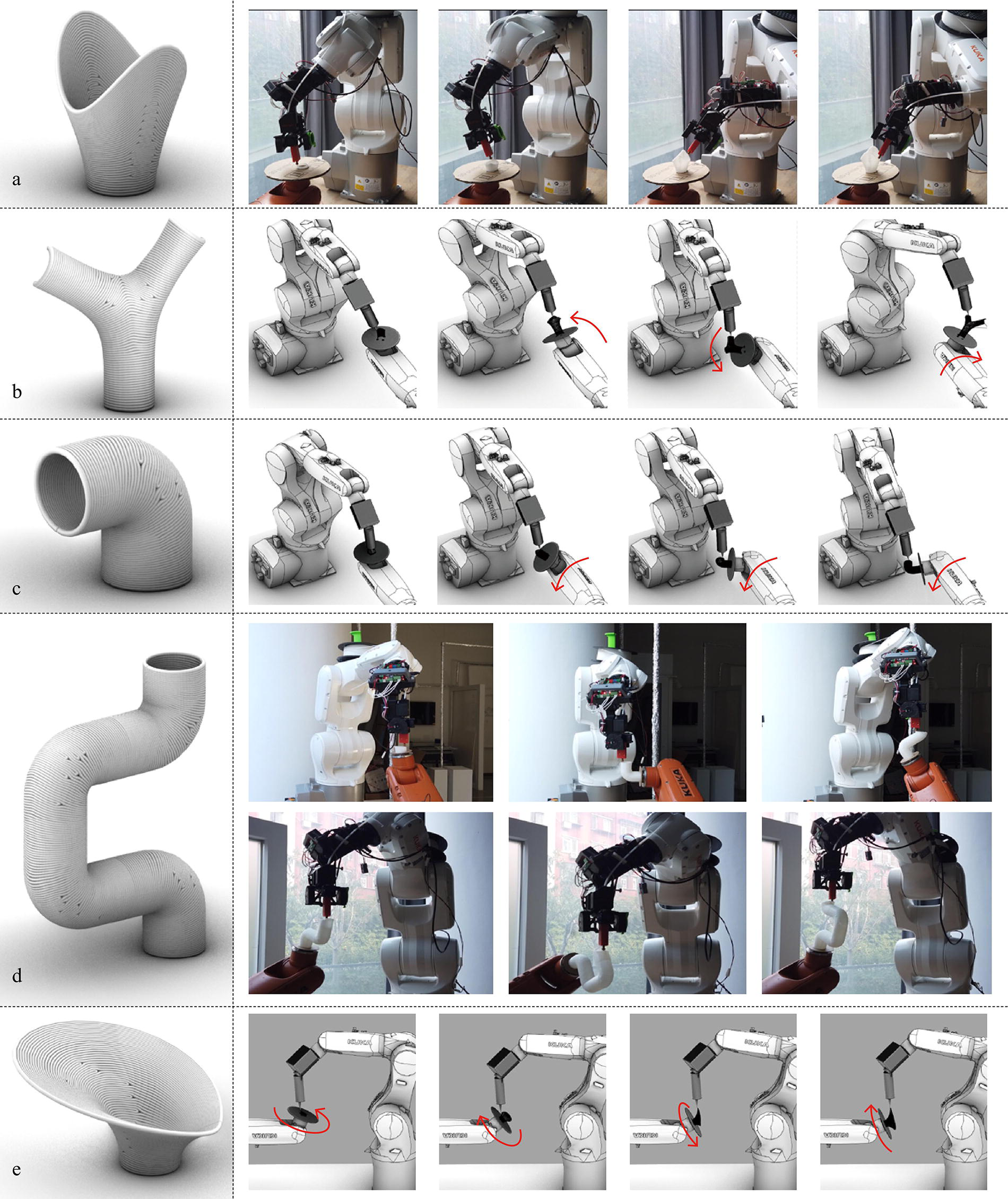
We can freeze Robot B in one pose when printing geometries with simple shapes. In this method, we appropriately move and rotate the World Origin Plane to get all turntable-Pln, which printhead-Pln can be derived based on (Fig. 7A). This printing method covers many types of surfaces like vases, irregular shells, structure components, and mutibranch connectors (Fig. 8A–F).

FIG. 7.

Path derivation and simulation.

FIG. 8.

Printing experiment results.

Method of Turntable Moving

The turntable needs to change poses over time when printing complex geometries. The method steps are as follows:

First, we divide the relative-Pln list into groups by orientation changes (Finer grouping ensures a vertical print head but the complex turntable movements). Second, we extract the average plane of every group as the reference plane. Third, we adjust the x-axis of the reference plane according to the spatial relationship. Fourth, we derive every changing result of the World Origin Plane when every reference plane adjusts vertically upwards. Finally, we move and rotate them appropriately to obtain turntable-Pln, deriving the printhead-Pln.

When printing geometries with only partial curvatures, the grouping of relative-Pln is needed only at the curvature-changing part (Fig. 7B), enabling printing workpieces such as connectors shown in (Fig. 8G, H).

When printing geometries with significant but gradual curvature, the turntable needs to move frequently, and the grouping of relative-Pln needs to be finer (Fig. 7C, D), suitable for bent connectors or pipes (Fig. 8I, J) such as vehicle structures.

When printing geometries with surrounding overhangs, the turntable needs continuous rotating. However, shaft limitation in the A6 axis of the robot is a difficulty. Therefore, a reciprocating printing path is chosen instead of a spiral ascent path (Fig. 7E), suitable for printing quasi-rotating bodies or overhanging cylindricals, such as hardware components.

Conclusion

This article proposes an extended method for single-shell nonplanar 3D printing. For path planning, this article proposes a path compensation method by distance field and a path homogenization method by dynamic relaxation to address the nonplanar printing path issue of uneven interlayer spacing. For robot 3D printing, this article proposes a dual-robot system and its path-derivation method to deal with highly curved printing path layers.

This method shows great potential for 3D printing single-shell surfaces with high curvatures or overhangs and opens up new possibilities for various applications in different manufacturing industries. We are committed to advancing this technology further and pushing the boundaries of additive manufacturing.

However, this study has some issues and limitations. Based on these, future solutions and directions for development are proposed:

Issues and solving ideas

Path planning. The compensation path often causes bloating or gaps at the folding position, resulting in uneven appearance and stress concentration of the material. In response to this, this research considers adjusting the physical parameters of the path at the turning position in the “Path Homogenization by Dynamic Relaxation” section to adjust its spacing. In addition, we also consider postprocessing methods such as polishing to deal with bloating.

Adhesion of objects. Extremely curved nonplanar layers require the turntable to tilt extremely, which might fall off the printed object, although this has not yet occurred. We can print additional adhesion plates at the bottom to address this.

Limitations and future development

Mechanical research limitations. This article lacks the verification of the mechanical properties of printed structures and the problem-solving on weak tangential strength of nonplanar printing. Therefore, we will conduct research and experimental verification of mechanical properties, think about more optimized processes, and add mechanical characterizations of the printed structure with and without your compensation algorithm in future studies.

Computational complexity. The computational complexity of the method is relatively high, especially for the dynamic relaxation during path homogenization. Regarding this, we have three ideas to alleviate: (a) Streamline redundant computing; (b) optimize a more uniform path compensation method; and (c) omit path homogenization because it is just an optimization step.

Materials and parameter standards. This article mainly focuses on the graphic study of path planning in FDM but does not delve into the material and the path compensation parameter standards. Therefore, we will research path compensation methods on more materials like plastics or metals and the parameter standards in the future, which will offer the potential for applications in industries such as automobiles and aerospace.

Path planning. This article only considers compensating for single-layer paths. In more extreme nonplanar paths, it may be necessary to consider whether to compensate for multilayer paths.

Dual-robot system. This article limits the turntable to some static limit orientations, lacking a universal derivation method utilizing the flexibility of the robots and the discussion on the effect of the robot’s DOF and configuration on printing. These will be involved in future research.

Authors’ Contributions

Z.S.: Conceptualization, data curation, formal analysis, investigation, methodology, software, validation, visualization, writing—original draft, and writing—review and editing. Q.C.: Conceptualization, funding acquisition, project administration, resources, supervision, validation, and writing—review and editing.

Footnotes

Author Disclosure Statement

The authors declare no conflicts of interest.

Funding Information

This study is supported by the China Postdoctoral Science Foundation under Grant Numbers 2023M742015 and 2024T170486.

References

Nisja

, Cao

, Gao

. Short review of nonplanar fused deposition modeling printing. Mat Design & Process Comms, 2021; 3(4):e221; doi: 10.1002/mdp2.221

Guidetti

, Balta

, Nagel

, et al. Stress flow guided non-planar print trajectory optimization for additive manufacturing of anisotropic polymers. Additive Manufact, 2023; 72:103628; doi: 10.1016/j.addma.2023.103628

, Li

, Chen

, et al. Curved layer based process planning for multi-axis volume printing of freeform parts. Computer-Aided Design, 2019; 114:51–63; doi: 10.1016/j.cad.2019.05.007

Knöppel

, Crane

, Pinkall

, et al. Stripe patterns on surfaces. ACM Trans Graph, 2015; 34(4):1–11; doi: 10.1145/2767000

Wang

, Zhang

, Hu

, et al. Research and implementation of a non-supporting 3D printing method based on 5-axis dynamic slice algorithm. Robot Comput Integr Manuf, 2019; 57:496–505; doi: 10.1016/j.rcim.2019.01.007

Coupek

, Friedrich

, Battran

, et al. Reduction of support structures and building time by optimized path planning algorithms in multi-axis additive manufacturing. Procedia Cirp, 2018; 67:221–226; doi: 10.1109/ICRA.2017.7989140

, Dai

, Fang

, et al. RoboFDM: A robotic system for support-free fabrication using FDM. 2017 IEEE Int Conf Robot Automation (ICRA), 2017:1175–1180; doi: 10.1109/ICRA.2017.7989140

Keating

, Oxman

. Compound fabrication: A multi-functional robotic platform for digital design and fabrication. Robotics and Computer-Integrated Manufacturing, 2013; 29(6):439–448; doi: 10.1016/j.rcim.2013.05.001

Mitropoulou

, Bernhard

, Dillenburger

. Print Paths Key-framing: Design for non-planar layered robotic FDM printing. In: Proceedings of the 5th annual ACM symposium on computational fabrication, 2020. pp. 1–10; doi: 10.1145/3424630.3425408

10.

Kout

, Müller

. Quantitative improvement of tool impact paths defined by isolines of scalar functions on triangular mesh workpiece surfaces. Int J Adv Manuf Technol, 2014; 70(1–4):237–255; doi: 10.1007/s00170-013-5250-6

11.

Dai

, Wang

, Wu

, et al. Support-free volume printing by multi-axis motion. ACM Trans Graph, 2018; 37(4):1–14; doi: 10.1145/3197517.3201342

12.

Shan

, Gan

, Mao

. Curved layer slicing based on isothermal surface. Procedia Manuf, 2021; 53:484–491; doi: 10.1016/j.promfg.2021.06.081

13.

, He

, Yuan

, et al. Vector field-based curved layer slicing and path planning for multi-axis printing. Robot Comp Integrated Manuf, 2022; 77:102362; doi: 10.1016/j.rcim.2022.102362

14.

Mitchell

JSB

, Mount

, Papadimitriou

. The discrete geodesic problem. SIAM J Comput, 1987; 16(4):647–668; doi: 10.1137/0216045

15.

Gediminas Kirdeikis: How to: Simple growth simulation (Grasshopper). Available from: https://www.youtube.com/watch?v=viEpaivq9A0 [Last accessed: September 3, 2024].

16.

Piker

. Kangaroo: Form finding with computational physics. Architectural Design, 2013; 83(2):136–137; doi: 10.1002/ad.1569

17.

Association for Robots in Architecture. KUKA|prc - Parametric robot control for grasshopper. Available from: https://www.robotsinarchitecture.org/kuka-prc [Last accessed: September 3, 2024].

18.

KUKA. KUKA roboteam. Available from: https://www.kuka.com/en-us/products/robotics-systems/software/hub-technologies/kuka_roboteam [Last accessed: September 3, 2024].