Toward a Topological Description of the Therapeutic Process

Abstract

Introduction:

Two (2) quantum theoretically based metaphor/models have been proposed recently to describe the therapeutic process in homeopathy in terms of (1) a representation of the vital force (Vf) as a spinning quantized gyroscope, describable as a wave function; and (2) a form of nonorthodox quantum theoretical entanglement (called PPR entanglement) between the patient, practitioner, and remedy.

Method:

Combining these two descriptions permits “normalization” of the Vf gyroscopic wave function. In this context, “normalization” refers to the probability of a patient's symptom totality being expressed and observable to the practitioner within a “therapeutic state space” that has mirror-like characteristics.

Results:

The Vf gyroscopic wave function contains a constant A related to this symptom totality and its expression. Normalization provides values for A at various stages of the patient's journey to cure, while at the same time suggesting a possible Möbius strip-like “topology” for the practitioner-derived “therapeutic state space.”

Conclusions:

Changes in the value of A on normalization indicate how expression of symptom totality varies at different stages of the patient's journey to cure, while suggesting a “topology” for the therapeutic process and how the practitioner could be affected by it.

Introduction

I n general, homeopathy is little regarded by biomedical scientists, and its growing evidence base has been dismissed out of hand.¹ This is due in part to the constantly fostered yet erroneous perception that any purported action of homeopathy's extremely diluted and agitated remedies cannot be explained within the known laws of science (see, however, the Memory of Water hypothesis and the current scientific evidence to support it).² Additionally, obtaining across-the-board agreement on trial reproducibility of homeopathic remedies is also perceived as difficult, even though in total, a sizeable majority of trials—around 60%—do show positive effects above and beyond placebo.³ The result is a built-in bias against homeopathy among those in the biomedical community, who tend to favor only negative homeopathic trial data,⁴ even when their collection and dissemination have themselves been shown to be fundamentally and systemically flawed.^5
–7 Clinical data supporting homeopathy are simply ignored.

Nevertheless, possible explanations for the efficacy of homeopathy have been developing in recent years, some using nonorthodox quantum theoretically based models of the therapeutic process. Not surprisingly, such models have met with much criticism and contempt from homeopathy's “detractors” (the term “skeptic” should be reserved for those who have yet to make up their minds), who largely adopt an exclusively orthodox (i.e., “realist”) ontology when interpreting quantum theory.⁸ This effectively confines any discussion of the subject to the realm of the incredibly small.

Thus, the orthodox interpretation of quantum theory assumes that a quantum state's mathematical formulation describes its objective physical reality. However, this view has been challenged by physicists such as Zeilinger, whose more recent interpretation of quantum theory considers the mathematical description of a quantum state to be only a representation of what can be known about it.⁹ Confirmation of such a view comes from d'Espagnet, who has concluded (based on quantum correlations between widely separated macroscopic systems, as discovered by Zeilinger) that we do not live in a strongly objective reality.¹⁰ In other words, in this interpretation of quantum theory, information takes on a more fundamental meaning than any notion of an “objective reality.” From this perspective, recent contempt shown toward the notion of entanglement between such seemingly qualitatively different, macroscopic entities as a remedy (derived from a material substance) and a totality of symptoms (an abstract idea generalized from one individual's observations about another), are based in a realist ontology.⁸ This presents a false dichotomy that disappears when it is realized that remedy and symptoms are, before anything, sources of information ¹¹ and their now similar ontology means they are quite capable of being “entangled” (via the practitioner) during the therapeutic process.¹² Though there is perhaps a gap between the pragmatism of orthodox quantum theory and use of its principles in the more metaphorical contexts described here, the above implies that the discourse of quantum theory is no longer confined to subatomic particles, atoms, molecules, and macroscopic systems derived from them. Indeed, via Weak Quantum Theory, such a discourse is beginning to have relevance in the description and understanding of nonphysical phenomena, such as the dynamics of interpersonal relations.¹³

Such a view could be said to be implicitly postmodern^14,15
* because by positing that what can be known about the world is intimately dependent on information derived from its observation,¹⁰ it effectively challenges the dominant “objectivist” scientific narrative (i.e., that reality exists “out there,” separate and independent of its observation, simply waiting to be discovered). On the contrary, reality “as it really is” is probably unknowable. Indeed, the idea of a knowable objective external reality is explicitly positivist and is the approach that is still dominant within the biomedical sciences in general, and among homeopathy's detractors in particular. Such a physicalist view is reductionist and arguably a reasonable approximation for most scientific purposes (e.g., the understanding of mechanistic structures and causal processes involved in such things as washing machines, bridges, and airplanes, etc.). It has even successfully explained the internal “workings” of living organisms, which have been reduced to known biochemical mechanistic pathways, such as the Krebs cycle.

However, in order to understand more subtle phenomena, such as complex interactions between living things (especially between human beings during the therapeutic process), a less reductionist approach could prove beneficial. That this may well resemble more ancient vitalistic (and holistic) traditions^16,17 will no doubt once again provoke strong negative responses from homeopathy's detractors who, steeped in a materialistic ontology, consider atavistic anything they think might smack of vitalism.

Thus, homeopathy's notion of the vital force (Vf) whose mode of action might be describable metaphorically in terms of something spinning, such that it has the propensity to “throw” morbific influences to the periphery of an organism, has been developed in a series of recent articles (specifically, the Vf has been modeled in terms of quantized gyroscopic motion and is therefore describable mathematically in terms of a potentially normalizable wave function).¹⁸ At the same time, a form of generalized quantum entanglement (between patient Px, practitioner Pr, and remedy Rx; known as PPR entanglement) has been invoked and elaborated as a possible metaphoric description of the curative interaction in homeopathy.¹⁹ It should be remembered that it is the discourse of quantum theory that is being used here to describe the Vf and the therapeutic process, not the orthodox quantum theory of subatomic particles, atoms, and molecules. In this context, the unorthodox use of quantum theory to describe macroscopic nonphysical phenomena has yet to be rigorously proven. This article will try to demonstrate that combining these two approaches allows normalization of the Vf wave function, which in turn suggests possible insights into how PPR entanglement elucidates different stages, and hence a “topology” of the curative homeopathic process.

PPR Entanglement Models Revisited (Box 1)^20

–23

Box 1. Defining Wave Functions for PPR Entanglement

From a previous mathematical approach, based on a model of the Vf behaving as a quantized gyroscopic,^17,20
–22 a wave function was developed describing a patient in an unwell state: \documentclass{aastex}\usepackage{amsbsy}\usepackage{amsfonts}\usepackage{amssymb}\usepackage{bm}\usepackage{mathrsfs}\usepackage{pifont}\usepackage{stmaryrd}\usepackage{textcomp}\usepackage{portland,xspace}\usepackage{amsmath,amsxtra}\pagestyle{empty}\DeclareMathSizes{10}{9}{7}{6} \begin{document} \begin{align*} \Psi_{\rm Vf} = 2{\rm Acosk}_{2}{\rm S}_{2} \tag {1} \end{align*} \end{document}

where S₂ represents the secondary symptom totality expressed by the patient, and the constant k₂ relates to factors representing the energy of the Vf “gyroscope.” The constant A relates to the amplitude of the Vf wave function, which in this context refers to the strength of symptoms and symptom expression (though it might also include information about the “signal/noise” ratio of the system). In addition, this approach describes a wave function for the remedy \documentclass{aastex}\usepackage{amsbsy}\usepackage{amsfonts}\usepackage{amssymb}\usepackage{bm}\usepackage{mathrsfs}\usepackage{pifont}\usepackage{stmaryrd}\usepackage{textcomp}\usepackage{portland,xspace}\usepackage{amsmath,amsxtra}\pagestyle{empty}\DeclareMathSizes{10}{9}{7}{6} \begin{document} \begin{align*} \Psi_{\rm Rx} = {\rm e}^{ - i{\rm k}_2 \Delta {\rm S}_2} \tag {2} \end{align*} \end{document}

where ΔS₂ represents the change in the patient's symptoms, wrought by the remedy. The best-case scenario is when all the symptoms disappear, and so the remedy covers all the patient's symptoms, (i.e., ΔS₂ = S₂). Under these circumstances: \documentclass{aastex}\usepackage{amsbsy}\usepackage{amsfonts}\usepackage{amssymb}\usepackage{bm}\usepackage{mathrsfs}\usepackage{pifont}\usepackage{stmaryrd}\usepackage{textcomp}\usepackage{portland,xspace}\usepackage{amsmath,amsxtra}\pagestyle{empty}\DeclareMathSizes{10}{9}{7}{6} \begin{document} \begin{align*} \Psi_{\rm Rx} = {\rm e}^{ - i{\rm k}_2 {\rm S}_2}. \tag {3} \end{align*} \end{document}

The worst-case scenario is when none of the symptoms disappear after consultation and remedy prescription, so the remedy covers none of the patient's symptoms (e.g., ΔS₂ = 0 and then Ψ_Rx↓ = 1). Also, from previous work on PPR entanglement,¹⁸ we have a set of equations describing the eight different states arising out of the patient (Px), the practitioner (Pr), and the remedy (Rx) undergoing three-way entanglement. These are: \documentclass{aastex}\usepackage{amsbsy}\usepackage{amsfonts}\usepackage{amssymb}\usepackage{bm}\usepackage{mathrsfs}\usepackage{pifont}\usepackage{stmaryrd}\usepackage{textcomp}\usepackage{portland,xspace}\usepackage{amsmath,amsxtra}\pagestyle{empty}\DeclareMathSizes{10}{9}{7}{6} \begin{document} \begin{align*} \mid \Psi_{\rm PPR} > \ = 1 / {\sqrt 2} (\mid \Psi_{{\rm Px} \uparrow} \cdot \Psi_{{\rm Pr} \uparrow} \cdot \Psi_{{\rm Rx} \uparrow} > \pm \ \mid \Psi_{{\rm Px} \downarrow} \cdot \Psi_{{ \rm Pr} \downarrow} \cdot \Psi_{{\rm Rx} \downarrow} >) \tag {4} \end{align*} \end{document} \documentclass{aastex}\usepackage{amsbsy}\usepackage{amsfonts}\usepackage{amssymb}\usepackage{bm}\usepackage{mathrsfs}\usepackage{pifont}\usepackage{stmaryrd}\usepackage{textcomp}\usepackage{portland,xspace}\usepackage{amsmath,amsxtra}\pagestyle{empty}\DeclareMathSizes{10}{9}{7}{6} \begin{document} \begin{align*} \mid \Psi_{\rm PPR} > \ = 1 / {\sqrt 2} (\mid \Psi_{{\rm Px} \uparrow} \cdot \Psi_{{\rm Pr} \uparrow} \cdot \Psi_{{\rm Rx} \downarrow} > \; \pm \; \mid \Psi_{{\rm Px} \downarrow} \cdot \Psi_{{\rm Pr} \downarrow} \cdot \Psi_{{\rm Rx} \uparrow} >) \tag {5} \end{align*} \end{document} \documentclass{aastex}\usepackage{amsbsy}\usepackage{amsfonts}\usepackage{amssymb}\usepackage{bm}\usepackage{mathrsfs}\usepackage{pifont}\usepackage{stmaryrd}\usepackage{textcomp}\usepackage{portland,xspace}\usepackage{amsmath,amsxtra}\pagestyle{empty}\DeclareMathSizes{10}{9}{7}{6} \begin{document} \begin{align*} \mid \Psi_{\rm PPR} > \ = 1 / {\sqrt 2} (\mid \Psi_{{\rm Px} \uparrow} \cdot \Psi_{{\rm Pr} \downarrow} \cdot \Psi_{{\rm Rx} \uparrow} > \ \pm \ \mid \Psi_{{\rm Px} \downarrow} \cdot \Psi_{{ \rm Pr} \uparrow} \cdot \Psi_{{\rm Rx} \downarrow} >) \tag {6} \end{align*} \end{document} \documentclass{aastex}\usepackage{amsbsy}\usepackage{amsfonts}\usepackage{amssymb}\usepackage{bm}\usepackage{mathrsfs}\usepackage{pifont}\usepackage{stmaryrd}\usepackage{textcomp}\usepackage{portland,xspace}\usepackage{amsmath,amsxtra}\pagestyle{empty}\DeclareMathSizes{10}{9}{7}{6} \begin{document} \begin{align*} \mid \Psi_{\rm PPR} > \ = 1 / {\sqrt 2} (\mid \Psi_{{\rm Px} \uparrow} \cdot \Psi_{{\rm Pr} \downarrow} \cdot \Psi_{{\rm Rx} \downarrow} > \ \pm \ \mid \Psi_{{\rm Px} \downarrow} \cdot \Psi_{{\rm Pr} \uparrow} \cdot \Psi_{{\rm Rx} \uparrow} >) \tag {7} \end{align*} \end{document}

These states are represented as vectors: normalization consists in combining each of these states with their complex conjugate, < Ψ_PPR| (i.e., < Ψ_PPR| Ψ_PPR>) to give scalars equal to 1, from which the value of A in equation 1 may be derived. Now, in 4-7, expressions have been derived for the patient and remedy wave functions (i.e., equations 1 and 3). In addition, this set of states is necessarily simplistic, involving only two sets of conditions. This leads to either the patient being cured or remaining unchanged after homeopathic intervention. Clearly, a more sophisticated analysis would need to be less stark and include states that are somewhere between these two extremes. Thus, up arrows mean the patient improved: the practitioner was helpful, and the remedy was effective in removing symptoms; down arrows mean the patient did not improve: the practitioner was unhelpful and the remedy was ineffective. Previous work provided an expression for the wave-function of an improved Vf (i.e., up arrow): \documentclass{aastex}\usepackage{amsbsy}\usepackage{amsfonts}\usepackage{amssymb}\usepackage{bm}\usepackage{mathrsfs}\usepackage{pifont}\usepackage{stmaryrd}\usepackage{textcomp}\usepackage{portland,xspace}\usepackage{amsmath,amsxtra}\pagestyle{empty}\DeclareMathSizes{10}{9}{7}{6} \begin{document} \begin{align*} \Psi_{{\rm Vf} + \Delta {\rm Vf}} = \Psi_{{\rm Px} \uparrow} = 2{\rm Acosk}_2 {\rm S}_2 \cdot {\rm e}^{ - i{\rm k}_2 \Delta { \rm S}_2}. \tag {8} \end{align*} \end{document}

Now during case-taking and repertorization, the practitioner tries to find a remedy that covers all the symptoms (i.e., ΔS₂ = S₂). Under these circumstances, equation 8 becomes:

\documentclass{aastex}\usepackage{amsbsy}\usepackage{amsfonts}\usepackage{amssymb}\usepackage{bm}\usepackage{mathrsfs}\usepackage{pifont}\usepackage{stmaryrd}\usepackage{textcomp}\usepackage{portland,xspace}\usepackage{amsmath,amsxtra}\pagestyle{empty}\DeclareMathSizes{10}{9}{7}{6} \begin{document} \begin{align*} \Psi_{{\rm Vf} + \Delta {\rm Vf}} = \Psi_{{\rm Px} \uparrow} = 2{\rm Acosk}_2 {\rm S}_2 \cdot {\rm e}^{ - i{\rm k}_2{\rm S}_2}. \tag {9} \end{align*} \end{document}

If on prescribing the remedy, the symptoms disappear (S₂ = 0 [i.e., the patient is restored to health]), then the improved patient wave function is represented by Ψ_Px↑ = 2A.

Similarly, if the remedy, Ψ_Rx, is curative (up arrow), then the change in symptoms it brings about covers all the secondary symptoms of the patient (i.e., ΔS₂ = S₂ and Ψ_Rx↑ = e^-ik₂ ^S₂). If the remedy is not curative (down arrow), and not all of the symptoms are covered, then simply ΔS₂ ≠ S₂, and Ψ_Rx↓ = e^-ik₂ ^ΔS₂. In the limit where the remedy covers none of the symptoms, ΔS₂ = 0 so that Ψ_Rx↓ = 1.

In considering how to represent the wave function of the practitioner Ψ_Pr, the action of the practitioner during entanglement may be likened to the provision of an “impulse” to the patient's Vf, which means that it might be describable in terms similar to the “impulse function” known from signal processing.²³ Such a wave function is known as the Kronecker or Dirac Δ function, which takes values of 1 (“helpful” practitioner Ψ_Pr↑) or 0 (“unhelpful” practitioner Ψ_Pr↓). \documentclass{aastex}\usepackage{amsbsy}\usepackage{amsfonts}\usepackage{amssymb}\usepackage{bm}\usepackage{mathrsfs}\usepackage{pifont}\usepackage{stmaryrd}\usepackage{textcomp}\usepackage{portland,xspace}\usepackage{amsmath,amsxtra}\pagestyle{empty}\DeclareMathSizes{10}{9}{7}{6} \begin{document} \begin{align*} \Psi_{{\rm Pr} \uparrow} = 1 \ {\rm and} \ \Psi_{{\rm Pr} \downarrow} = 0. \tag {10} \end{align*} \end{document}

Gyroscopic model¹⁸

The Vf is imagined as behaving in a way similar to a gyroscope. This is because a spinning object exerts a centripetal force on anything attached to it, which tends to throw it outward: the Vf is thought to act similarly in resisting stressors, by throwing them outward to the organism's extremities.

In its simplest form, a gyroscope consists of a spinning “flywheel” within a bearing-containing frame. When the flywheel is set spinning, the gyroscope stands upright against the downward pull of gravity, and resists strongly any force that attempts to push it over. As the flywheel slows, however, its spinning axis itself begins to wobble and eventually tilts over, ceasing to point directly upward, but instead slowly rotating about the vertical. This is called precession, and the continued slowing of the gyroscope's flywheel means that as precession increases, the gyroscope is less resistant to forces that would push it over. Far more complex versions of the gyroscope (in which flywheels are kept spinning at maximum revolutions) are used to stabilize spacecraft, guided weaponry, and ocean-going vessels, etc.

In using the gyroscope as an analogy for the Vf, we consider that its “flywheel” is slowed discreetly by disease, causing it to “precess” about an imaginary vertical axis: This precession would be experienced as the exhibition of the symptoms of disease, and it would change by fixed (quantized) amounts. Similarly, remedies increase discreetly the “flywheel's” rate of spin, reducing the Vf gyroscope's “precession,” and so removing the symptoms. In this regard, it becomes possible to describe the Vf in terms of a quantized gyroscopic “wave function,” which equates the strength of symptom expression to the degree of Vf gyroscopic “precession.” Such an expression for the patient in an unwell state (see Box 1, equation 1: Ψ_Vf = 2Acosk₂S₂) allows diseases and homeopathic remedies to be seen in terms of a mirror-image relationship, interpreted respectively as braking and accelerating “torques” on Vf precessional “angular momentum.” It remains to be seen whether future work can reveal the subtlety of the relationship between a remedy at a particular potency and the change this produces to the Vf “angular momentum.”

These ideas have been used to illustrate some of homeopathy's empirical laws (e.g., biphasal action of remedies),²⁴ and resonance effects among remedy provers and their associates.²⁰ A therapeutic analogue of the time-dependent Schrödinger equation has also been used to investigate the practitioner's effect on the patient's Vf during therapeutic patient–practitioner–remedy entanglement.²⁵

PPR entanglement model¹⁹

Recent attempts to explain homeopathy's efficacy have made use of concepts generalized from the discourses of semiotics^26,27 and quantum theory.^28
–30 Thus, nonlocal coherence^12,13,31 between patient (Px), practitioner (Pr), and remedy (Rx) known as PPR entanglement, forms a descriptive basis from which to describe the healing interaction in mathematical terms.^32

–37 It combines the algebraic formalism of Greenberger–Horne–Zeilinger three-particle entanglement,³⁸ a generalization of orthodox quantum theory to nonphysical macroscopic systems called Weak Quantum Theory,^12,13 and semiotics^26,27 to generate a three-way PPR entangled state. This has been depicted geometrically as a tetrahedron, with the process of cure being visualized—again geometrically and metaphorically—as resulting from the combination of this state with its “twisted reflection” in a notional two-dimensional mirror-like “therapeutic state-space” (an analogue of the complex mathematical Hilbert space more familiar from orthodox quantum theory), to produce a stellated octahedron.¹⁹ Though at this stage still hypothetical and still to be rigorously proven, PPR entanglement affords a post hoc explanation³⁹ of the observed “leakage” between verum and placebo groups during recent double-blind provings of homeopathic remedies,^40

–43 suggesting its possible experimental verification. In addition, and when viewed semiotically, the PPR entangled state's geometrical projection into a notional “therapeutic state space” has been used to understand the concept of miasms in homeopathy,⁴⁴ and the action of remedies and diseases on the Vf.¹⁸ The purpose of this article is to investigate further the “semiotic geometry” of the PPR entangled state,¹⁹ and to deepen insight into the complex therapeutic interaction of the patient, practitioner, and the remedy on the way to cure. It confirms that the practitioner may facilitate but ultimately does not control this process.

Normalization of the Patient's Vf Wave Function (Box 2)⁴⁵

Box 2. Normalization and the Patient Vf Wave Function

So, in general, if Ψ is a complex wave function (i.e., is composed of complex numbers that in turn are composites of a real number part and an imaginary number part, based on i = √-1),⁴⁵ then Ψ* is its complex conjugate. A property of complex numbers is that when they are multiplied by their complex conjugates, the product is a real number. In quantum theory, the product of Ψ and Ψ* \documentclass{aastex}\usepackage{amsbsy}\usepackage{amsfonts}\usepackage{amssymb}\usepackage{bm}\usepackage{mathrsfs}\usepackage{pifont}\usepackage{stmaryrd}\usepackage{textcomp}\usepackage{portland,xspace}\usepackage{amsmath,amsxtra}\pagestyle{empty}\DeclareMathSizes{10}{9}{7}{6} \begin{document} \begin{align*} \psi \cdot \psi^* = \mid \psi \mid ^{2} \end{align*} \end{document}

also represents a real number, which is greater than or equal to zero, and is known as the probability density function. This means that \documentclass{aastex}\usepackage{amsbsy}\usepackage{amsfonts}\usepackage{amssymb}\usepackage{bm}\usepackage{mathrsfs}\usepackage{pifont}\usepackage{stmaryrd}\usepackage{textcomp}\usepackage{portland,xspace}\usepackage{amsmath,amsxtra}\pagestyle{empty}\DeclareMathSizes{10}{9}{7}{6} \begin{document} \begin{align*} p (- \infty \le x \le \infty) = \int \mid \psi \mid ^{2}dx \,( \rm{between\ the\ values} \ \infty \ {\rm and} \ - \infty) \tag {a} \end{align*} \end{document}

where p(x) is the probability of finding the particle at a point in space x. Equation (a) is given by the definition of a probability density function. Since the particle exists, the probability of it being somewhere in space must be 100% (i.e., equal to 1). Therefore, integrating over all space (i.e., between ∞ and −∞ ) gives:

\documentclass{aastex}\usepackage{amsbsy}\usepackage{amsfonts}\usepackage{amssymb}\usepackage{bm}\usepackage{mathrsfs}\usepackage{pifont}\usepackage{stmaryrd}\usepackage{textcomp}\usepackage{portland,xspace}\usepackage{amsmath,amsxtra}\pagestyle{empty}\DeclareMathSizes{10}{9}{7}{6} \begin{document} \begin{align*} p (- \infty \le x \le \infty) = \int \mid \psi \mid ^{2}dx = 1 \tag {b} \end{align*} \end{document}

A shorthand way of representing equation (b) (using the bra-ket notation invented by the British physicist P.A.M. Dirac)²¹ is: \documentclass{aastex}\usepackage{amsbsy}\usepackage{amsfonts}\usepackage{amssymb}\usepackage{bm}\usepackage{mathrsfs}\usepackage{pifont}\usepackage{stmaryrd}\usepackage{textcomp}\usepackage{portland,xspace}\usepackage{amsmath,amsxtra}\pagestyle{empty}\DeclareMathSizes{10}{9}{7}{6} \begin{document} \begin{align*}< \psi \mid \psi > = 1 \tag {c} \end{align*} \end{document}

If the integral is finite, the wave function Ψ may be multiplied by a constant such that the integral is equal to 1. Alternatively, if the wave function already contains an appropriate arbitrary constant, equation (b) or (c) can be solved to find the value of this constant, which normalizes the wave function.

Now we are in a position to normalize the PPR entangled states given in equations (4 –7), and so derive values for the constant A in the patient's Vf wave function. Consider equation (4), for example. Normalization gives: \documentclass{aastex}\usepackage{amsbsy}\usepackage{amsfonts}\usepackage{amssymb}\usepackage{bm}\usepackage{mathrsfs}\usepackage{pifont}\usepackage{stmaryrd}\usepackage{textcomp}\usepackage{portland,xspace}\usepackage{amsmath,amsxtra}\pagestyle{empty}\DeclareMathSizes{10}{9}{7}{6} \begin{document} \begin{align*}< \Psi_{\rm PPR} \mid \Psi_{\rm PPR} > &= 1 / {2} [ (< \Psi_{{ \rm Px} \uparrow} \cdot \Psi_{{\rm Pr} \uparrow} \cdot \Psi_{{ \rm Rx} \uparrow}\mid \Psi_{{\rm Px} \uparrow} \cdot \Psi_{{\rm Pr} \uparrow} \cdot \Psi_{{\rm Rx} \uparrow} >) \pm (< \Psi_{{ \rm Px} \uparrow} \cdot \Psi_{{\rm Pr} \uparrow} \cdot \Psi_{{ \rm Rx} \uparrow}\mid \Psi_{{\rm Px} \downarrow} \cdot \Psi_{{ \rm Pr} \downarrow} \cdot \Psi_{{\rm Rx} \downarrow} >) \\&\quad\pm (< \Psi_{{\rm Px} \downarrow} \cdot \Psi_{{\rm Pr} \downarrow} \cdot \Psi_{{\rm Rx} \downarrow}\mid \Psi_{{\rm Px} \downarrow} \cdot \Psi_{{\rm Pr} \downarrow} \cdot \Psi_{{\rm Rx} \downarrow} >) \pm (< \Psi_{{\rm Px} \downarrow} \cdot \Psi_{{\rm Pr} \downarrow} \cdot \Psi_{{\rm Rx} \downarrow}\mid \Psi_{{\rm Px} \uparrow} \cdot \Psi_{{\rm Pr} \uparrow} \cdot \Psi_{{\rm Rx} \uparrow} >) ] = 1 \tag {11} \end{align*} \end{document}

Similar normalization equations can be written using (5 –7). Inspecting these (and because Ψ_Pr↓ = 0), three of the terms in each of the normalization equations will cancel out. There are, however, several steps to consider during PPR entanglement. The first is when the practitioner has taken the patient's case and found a remedy that covers all of the possible symptoms (i.e., when ΔS₂ = S₂), and the second is when all symptoms have been removed (i.e., when S₂ → 0).

Step 1 : “Mirror; mirror on the wall … .”: covering the symptoms; ΔS₂ = S₂ .

Considering the PPR entangled state from equation (4), and substituting Ψ_Px↑ = 2Acosk₂S₂.e^−ik₂ ^S₂; Ψ_Pr↑ = 1; Ψ_Rx↑ = e^−ik₂ ^S₂; Ψ_Px↓ = 2Acosk₂S₂; Ψ_Pr↓ = 0, and Ψ_Rx↓ = e^−ik₂ ^ΔS₂ (and complex conjugates) into equation (11) gives: \documentclass{aastex}\usepackage{amsbsy}\usepackage{amsfonts}\usepackage{amssymb}\usepackage{bm}\usepackage{mathrsfs}\usepackage{pifont}\usepackage{stmaryrd}\usepackage{textcomp}\usepackage{portland,xspace}\usepackage{amsmath,amsxtra}\pagestyle{empty}\DeclareMathSizes{10}{9}{7}{6} \begin{document} \begin{align*}< \Psi_{\rm PPR} \mid \Psi_{\rm PPR} > = 1 / 2 \int ( \{ 2{\rm Acosk}_2 {\rm S}_2 \cdot {\rm e}^{i{\rm k}_2 {\rm S}_{2.1}} \cdot {\rm e}^{i {\rm k}_2 {\rm S}_2}\} \{{2{\rm Acosk}_2 {\rm S}_2 \cdot {\rm e}^{ - i{\rm k}_2 {\rm S}_{2\cdot 1}}} \cdot { \rm e}^{ - i{\rm k}_2 {\rm S_2}}\}) {\rm dS}_2 = 1 \end{align*} \end{document}

Therefore: \documentclass{aastex}\usepackage{amsbsy}\usepackage{amsfonts}\usepackage{amssymb}\usepackage{bm}\usepackage{mathrsfs}\usepackage{pifont}\usepackage{stmaryrd}\usepackage{textcomp}\usepackage{portland,xspace}\usepackage{amsmath,amsxtra}\pagestyle{empty}\DeclareMathSizes{10}{9}{7}{6} \begin{document} \begin{align*}< \Psi_{\rm PPR} \mid \Psi_{\rm PPR} > = 1 / 2 \int4{\rm A}^{2} \cos^2{\rm k}_2{\rm S}_2 \cdot {\rm dS}_{2} = 1; \ {\rm and} , \quad[ 2{\rm A}^2 \cdot {\rm S}_2 / 2 ] = 1. \end{align*} \end{document}

The range of integration now has to be determined. In previous articles¹⁸ it was stated that the practitioner acts as a mirror for the patient. This would mean the therapeutic “state-space” in which symptoms “appear” for practitioner observation is in essence a 2-D mirror plane. The range of integration should be therefore from 0 to 2π. Consequently: \documentclass{aastex}\usepackage{amsbsy}\usepackage{amsfonts}\usepackage{amssymb}\usepackage{bm}\usepackage{mathrsfs}\usepackage{pifont}\usepackage{stmaryrd}\usepackage{textcomp}\usepackage{portland,xspace}\usepackage{amsmath,amsxtra}\pagestyle{empty}\DeclareMathSizes{10}{9}{7}{6} \begin{document} \begin{align*} [2{\rm A}^{2} \cdot \pi ] = 1 , \ {\rm and} \quad\ \underline{{ \rm A} = 1 / {\sqrt 2 \pi} \approx 0.4}. \end{align*} \end{document}

Now, a similar inspection of equations (5 –7), followed by normalization delivers the same result: \documentclass{aastex}\usepackage{amsbsy}\usepackage{amsfonts}\usepackage{amssymb}\usepackage{bm}\usepackage{mathrsfs}\usepackage{pifont}\usepackage{stmaryrd}\usepackage{textcomp}\usepackage{portland,xspace}\usepackage{amsmath,amsxtra}\pagestyle{empty}\DeclareMathSizes{10}{9}{7}{6}\begin{document}$${\rm A} = 1 / {\sqrt 2 \pi}$$\end{document} .

Step 2 : “Let the dog see the rabbit … .”: removing the symptoms; S₂ → 0.

Considering the PPR entangled state from equation (4), and substituting Ψ_Px↑ = 2A; Ψ_Pr↑ = 1; Ψ_Rx↑ = 1; Ψ_Px↓ = 2Acosk₂S₂; Ψ_Pr↓ = 0, and Ψ_Rx↓ = e^-ik₂ ^ΔS₂ (and their complex conjugates) into equation (11) gives: \documentclass{aastex}\usepackage{amsbsy}\usepackage{amsfonts}\usepackage{amssymb}\usepackage{bm}\usepackage{mathrsfs}\usepackage{pifont}\usepackage{stmaryrd}\usepackage{textcomp}\usepackage{portland,xspace}\usepackage{amsmath,amsxtra}\pagestyle{empty}\DeclareMathSizes{10}{9}{7}{6} \begin{document} \begin{align*}< \Psi_{\rm PPR} \mid \Psi_{\rm PPR} > = 1 / 2 \int ( \{ 2{\rm A} \cdot {\rm e}^{i{\rm k_2 \rm S_{2.1}}} \cdot {\rm e}^{i{\rm k_2 \rm S_2}} \} \{ 2{\rm A} \cdot {\rm e}^{ - i{\rm k_2 \rm S_{2.1}}} \cdot {\rm e}^{ - ik_2 \rm S_2} \}) {\rm dS}_2 = 1 \end{align*} \end{document} \documentclass{aastex}\usepackage{amsbsy}\usepackage{amsfonts}\usepackage{amssymb}\usepackage{bm}\usepackage{mathrsfs}\usepackage{pifont}\usepackage{stmaryrd}\usepackage{textcomp}\usepackage{portland,xspace}\usepackage{amsmath,amsxtra}\pagestyle{empty}\DeclareMathSizes{10}{9}{7}{6} \begin{document} \begin{align*}< \Psi_{\rm PPR} \mid \Psi_{\rm PPR} > = 1 / 2 \int ( \{ 2{\rm A}.1. 1 \} \{ 2{\rm A}.1.1 \}) {\rm dS}_2 = 1 \end{align*} \end{document}

And again integrating between 0 to 2π gives \documentclass{aastex}\usepackage{amsbsy}\usepackage{amsfonts}\usepackage{amssymb}\usepackage{bm}\usepackage{mathrsfs}\usepackage{pifont}\usepackage{stmaryrd}\usepackage{textcomp}\usepackage{portland,xspace}\usepackage{amsmath,amsxtra}\pagestyle{empty}\DeclareMathSizes{10}{9}{7}{6} \begin{document} \begin{align*} 1 / {2} \int 4{\rm A}^{2} \cdot {\rm dS}_{2} = [ 2{\rm A}^2 \cdot {\rm S}_2 ] = 1 \cdot [ 2{\rm A}^2 \cdot 2 \pi ] = 1 , \ { \rm and} \quad\ \underline{{\rm A} = 1 / {2 \sqrt \pi} \approx 0.282}. \end{align*} \end{document}

Inspecting equation (5) and normalizing as in equation (11) delivers the same result; \documentclass{aastex}\usepackage{amsbsy}\usepackage{amsfonts}\usepackage{amssymb}\usepackage{bm}\usepackage{mathrsfs}\usepackage{pifont}\usepackage{stmaryrd}\usepackage{textcomp}\usepackage{portland,xspace}\usepackage{amsmath,amsxtra}\pagestyle{empty}\DeclareMathSizes{10}{9}{7}{6}\begin{document}$${\rm A} = 1 / {2 \sqrt \pi}$$\end{document} . However, similar inspection of equations (6) and (7) and then normalization via equation (11) gives \documentclass{aastex}\usepackage{amsbsy}\usepackage{amsfonts}\usepackage{amssymb}\usepackage{bm}\usepackage{mathrsfs}\usepackage{pifont}\usepackage{stmaryrd}\usepackage{textcomp}\usepackage{portland,xspace}\usepackage{amsmath,amsxtra}\pagestyle{empty}\DeclareMathSizes{10}{9}{7}{6}\begin{document}$${\rm A} = 1 / {\sqrt 2 \pi}$$\end{document} , as in step 1 above. In (4) and (5) the patient and the practitioner are both up arrowed (i.e., they may be considered as entangled “in synch” with each other), so that \documentclass{aastex}\usepackage{amsbsy}\usepackage{amsfonts}\usepackage{amssymb}\usepackage{bm}\usepackage{mathrsfs}\usepackage{pifont}\usepackage{stmaryrd}\usepackage{textcomp}\usepackage{portland,xspace}\usepackage{amsmath,amsxtra}\pagestyle{empty}\DeclareMathSizes{10}{9}{7}{6}\begin{document}$${\rm A} = 1 / {2 \sqrt \pi} \approx 0.282$$\end{document} , while in (6) and (7) the patient and practitioner are alternately up and down arrowed (i.e., entangled “out of synch” with each other) and give \documentclass{aastex}\usepackage{amsbsy}\usepackage{amsfonts}\usepackage{amssymb}\usepackage{bm}\usepackage{mathrsfs}\usepackage{pifont}\usepackage{stmaryrd}\usepackage{textcomp}\usepackage{portland,xspace}\usepackage{amsmath,amsxtra}\pagestyle{empty}\DeclareMathSizes{10}{9}{7}{6}\begin{document}$${\rm A} = 1 / {\sqrt 2 \pi} \approx 0.4$$\end{document} .

Step 3 : “ … Through the looking glass … .”: post-entanglement self-super-position

After PPR entanglement, self-superposition⁴⁷ (a realization of the patient's well and unwell states) leads to a further reduction in the value of A on normalization. This could be represented as: \documentclass{aastex}\usepackage{amsbsy}\usepackage{amsfonts}\usepackage{amssymb}\usepackage{bm}\usepackage{mathrsfs}\usepackage{pifont}\usepackage{stmaryrd}\usepackage{textcomp}\usepackage{portland,xspace}\usepackage{amsmath,amsxtra}\pagestyle{empty}\DeclareMathSizes{10}{9}{7}{6} \begin{document} \begin{align*} \mid\Psi_{Px} > = 1 / {\sqrt 2} (\mid \Psi_{{\rm Px} \uparrow}> \ \pm \ \mid \Psi_{{\rm Px} \downarrow} >) \tag {12} \end{align*} \end{document} \documentclass{aastex}\usepackage{amsbsy}\usepackage{amsfonts}\usepackage{amssymb}\usepackage{bm}\usepackage{mathrsfs}\usepackage{pifont}\usepackage{stmaryrd}\usepackage{textcomp}\usepackage{portland,xspace}\usepackage{amsmath,amsxtra}\pagestyle{empty}\DeclareMathSizes{10}{9}{7}{6} \begin{document} \begin{align*}{\rm and} \ &< \Psi_{\rm Px} \mid \Psi_{\rm Px} > = 1 / 2 (< \Psi_{{\rm Px} \uparrow}\mid \ \pm \ < \Psi_{{\rm Px} \downarrow}\mid) (\mid \Psi_{{\rm Px} \uparrow} > \ \pm \ \mid \Psi_{{\rm Px} \downarrow} >) = 1 / 2 (< \Psi_{{\rm Px} \uparrow}\mid \Psi_{{\rm Px} \uparrow} > \\\quad\pm &< \Psi_{{ \rm Px} \uparrow}\mid \Psi_{{\rm Px} \downarrow} > \pm < \Psi_{{ \rm Px} \downarrow}\mid \Psi_{{\rm Px} \downarrow} > \pm < \Psi_{{\rm Px} \downarrow}\mid \Psi_{{\rm Px} \uparrow} >) = 1 \end{align*} \end{document}

“Well patient” is |Ψ_Px↑ > = 2A; “unwell” patient Ψ_Pr↓ = 2Acosk₂S₂: so, substituting normalizing and integrating: \documentclass{aastex}\usepackage{amsbsy}\usepackage{amsfonts}\usepackage{amssymb}\usepackage{bm}\usepackage{mathrsfs}\usepackage{pifont}\usepackage{stmaryrd}\usepackage{textcomp}\usepackage{portland,xspace}\usepackage{amsmath,amsxtra}\pagestyle{empty}\DeclareMathSizes{10}{9}{7}{6} \begin{document} \begin{align*}< \Psi_{\rm Px} \mid \Psi_{\rm Px} > = 1 / 2 \int 4{\rm A}^{2}(1 \pm 2{\rm cosk}_2{\rm S}_{2} \ + \ \cos^2{\rm k}_2{\rm S}_2) \cdot {\rm dS}_2 = 2{\rm A}^2 [ {\rm S}_2 \ \pm \ {2 / \rm k_2}{\rm sink}_2{\rm S}_2 + {\rm S}_2 / 2 ] = 1; \ \quad{ \rm and} \ \underline{{\rm A} = 1 / {\sqrt{6} \pi}} \end{align*} \end{document}

Normalization in the therapeutic context

In orthodox quantum theory, wave functions represent real particles and they must be normalizable.⁴⁶ This is a standard technique used by physicists and mathematicians to scale the numbers they are working with to a convenient size, so that they can be easily represented (e.g., graphically). For wave functions, it results in the probability of the particle existing (and so occupying any place in all of space) being 100% (usually said to be equal to 1). This means that it is then possible to acquire a value for the amplitude of the wave function (the constant in front of the wave function) for a particle or system of particles.

Of course, in considering the patient's Vf wave function, which is a nonorthodox quantum theoretical definition (Ψ_Vf = 2Acosk₂S₂), it does not represent anything physically “real” (e.g., a particle or a human being) in the materialistically objective sense as understood by orthodox quantum theory. However, in terms of the more recent interpretation of quantum theory mentioned earlier (which considers the mathematical description of a quantum state to be only a representation of what can be known about it),^9,10 Ψ_Vf refers to the patient as a source of information accessed by the practitioner during case-taking. Yet Ψ_Vf contains a constant A that relates to its “amplitude” and so mathematically, the wave function should be normalizable. The question then is what would normalization mean in the context of the therapeutic homeopathic interaction, and in what mathematical “space” normalization takes place.

Inspection of Ψ_Vf shows that it is dependent on the patient's expressed symptom totality S₂ as observed by the practitioner during the therapeutic process. Ψ_Vf is also related to a constant k₂, which is dependent on the energy of the patient's Vf.^18,25 So, as in equations (b) and (c) in Box 2, integrating the product of Ψ_Vf and its complex conjugate Ψ_Vf* over the therapeutic state space (which, as has been described previously, is envisioned as a two-dimensional [2-D] mirror-like “plane,” so that the range of integration is therefore between 0 and 2π),¹⁸ could have meaning in relation to the probability of the patient's symptoms being observable by the practitioner during the consultation and is set equal to 1. Being related to the amplitude of the patient's Vf wave function (itself imagined as a quantized, precessing [i.e., symptom-expressing] gyroscope),^22,23 the numerical value of the constant A derived from normalization could be thought to represent the magnitude of expression of the observed symptoms, and this value changes through the various stages of the therapeutic process, rising to a maximum before decreasing after therapeutic PPR entanglement (Fig. 1, black bars and arrows).

FIG. 1.

Vital force (Vf) “normalization profile” before, during, and after generalized quantum entanglement between patient Px, practitioner Pr, and remedy Rx (PPR entanglement). The gray area represents the “zone” of entanglement between patient, practitioner, and remedy and possible outcomes. Symptom reduction corresponds to reduction in the value A. Thus, on “in-synch” PPR entanglement (corresponding to equations 4 and 5, Box 1), A for the patient starts high (C1; increasing initially from A to B), then decreases (D1), while A′ for the practitioner starts low (C2), the increases (D2). However, on “out-of-synch” PPR entanglement (corresponding to equations 6 and 7; Box 1), A remains high (D2), and stays low (C2). Ultimately, during the journey to cure, both A and A′ return to lower levels (E and F). This is not meant to imply A′ for the practitioner fluctuates and changes to the same extent as A for the patient: rather, it is a crude representation of how patient and practitioner Vf's might interact, reminiscent of expectation and transference/countertransference phenomena well known in other therapeutic modalities.⁵⁴

Normalization of the patient Vf wave function

The mathematical derivation is developed through Boxes 2 and 3. The basic premise of therapeutic entanglement between patient (Px), practitioner (Pr), and remedy/therapeutic modality (Rx) is that they may each be considered sources of information represented as wave functions (Ψ_Px = Ψ_Vf, Ψ_Pr, and Ψ_Rx, respectively: simplistically, the practitioner may be “helpful” or “unhelpful”; the remedy “curative” or “noncurative,” and the patient “well” or “unwell,” each of these states represented by an up or down arrow, respectively; see Box 1) that define what can be known about each of them. As wave functions they can undergo various overlapping interactions, such as superposition, to produce entangled states dependent on whether the practitioner is “helpful” or “unhelpful.” Here, Ψ_Pr may be envisaged as behaving like a Kronecker delta function,⁴⁷ taking the values 1 or 0. In signal processing, the Kronecker delta function is also referred to as a unit impulse provided for systems working in discrete time. Used in the therapeutic context, the practitioner may be thought of as providing an “impulse” (or not; taking values 1 or 0, respectively) to the patient in the “discrete time” of the consultation. The practitioner's “impulse response” is therefore complex, depending on the practitioner and the remedy.

Box 3. Changing Values for the Constant A on Normalization

The treatment in Box 2 suggests that the normalization value of A in the patient wave-function can take several different values. These differences correspond to changes in the amplitude of the patient wave function, beginning with a minimum value of A corresponding to a patient with a healthier Vf. These differences in A are most likely indicators of changes in the strength of expression of the patient's observed symptoms.

Thus, using the same normalization protocol as in Box 2, the individual “well” and “unwell” patient wave functions (i.e., respectively, Ψ_Px↑ = 2A and Ψ_Px↓ = 2Acosk₂S₂) give increasing values of \documentclass{aastex}\usepackage{amsbsy}\usepackage{amsfonts}\usepackage{amssymb}\usepackage{bm}\usepackage{mathrsfs}\usepackage{pifont}\usepackage{stmaryrd}\usepackage{textcomp}\usepackage{portland,xspace}\usepackage{amsmath,amsxtra}\pagestyle{empty}\DeclareMathSizes{10}{9}{7}{6}\begin{document}$${\rm A} = 1 / {2 \sqrt 2 \pi}$$\end{document} and \documentclass{aastex}\usepackage{amsbsy}\usepackage{amsfonts}\usepackage{amssymb}\usepackage{bm}\usepackage{mathrsfs}\usepackage{pifont}\usepackage{stmaryrd}\usepackage{textcomp}\usepackage{portland,xspace}\usepackage{amsmath,amsxtra}\pagestyle{empty}\DeclareMathSizes{10}{9}{7}{6}\begin{document}$$1 / {2 \sqrt \pi}$$\end{document} . The value of A then increases again (Fig. 1; black bars and arrows) to a maximum in step 1 of PPR entanglement during case taking, when the patient's “disease” and a remedy that could cover all the patient's symptoms are elaborated: ΔS₂ = S₂ and \documentclass{aastex}\usepackage{amsbsy}\usepackage{amsfonts}\usepackage{amssymb}\usepackage{bm}\usepackage{mathrsfs}\usepackage{pifont}\usepackage{stmaryrd}\usepackage{textcomp}\usepackage{portland,xspace}\usepackage{amsmath,amsxtra}\pagestyle{empty}\DeclareMathSizes{10}{9}{7}{6}\begin{document}$${\rm A} = 1 / {\sqrt 2 \pi}$$\end{document} . In step 2, PPR entanglement continues and the symptoms are removed S₂ → 0, but only if the practitioner entangles “in synch” with the patient does the value of A come back down to \documentclass{aastex}\usepackage{amsbsy}\usepackage{amsfonts}\usepackage{amssymb}\usepackage{bm}\usepackage{mathrsfs}\usepackage{pifont}\usepackage{stmaryrd}\usepackage{textcomp}\usepackage{portland,xspace}\usepackage{amsmath,amsxtra}\pagestyle{empty}\DeclareMathSizes{10}{9}{7}{6}\begin{document}$$1 / {2 \sqrt \pi}$$\end{document} . If the practitioner is out “of synch” with the patient, the value of A remains the same at \documentclass{aastex}\usepackage{amsbsy}\usepackage{amsfonts}\usepackage{amssymb}\usepackage{bm}\usepackage{mathrsfs}\usepackage{pifont}\usepackage{stmaryrd}\usepackage{textcomp}\usepackage{portland,xspace}\usepackage{amsmath,amsxtra}\pagestyle{empty}\DeclareMathSizes{10}{9}{7}{6}\begin{document}$$1 / {\sqrt 2 \pi}$$\end{document} . In step 3, the patient undergoes “self-superposition” (realizing of their well and unwell states), leading to a further reduction in the value of A; to \documentclass{aastex}\usepackage{amsbsy}\usepackage{amsfonts}\usepackage{amssymb}\usepackage{bm}\usepackage{mathrsfs}\usepackage{pifont}\usepackage{stmaryrd}\usepackage{textcomp}\usepackage{portland,xspace}\usepackage{amsmath,amsxtra}\pagestyle{empty}\DeclareMathSizes{10}{9}{7}{6}\begin{document}$$1 / {\sqrt 6 \pi}$$\end{document} . Finally, the value of A returns to its starting value ( \documentclass{aastex}\usepackage{amsbsy}\usepackage{amsfonts}\usepackage{amssymb}\usepackage{bm}\usepackage{mathrsfs}\usepackage{pifont}\usepackage{stmaryrd}\usepackage{textcomp}\usepackage{portland,xspace}\usepackage{amsmath,amsxtra}\pagestyle{empty}\DeclareMathSizes{10}{9}{7}{6}\begin{document}$$1 / {2 \sqrt 2 \pi}$$\end{document} ) for a well-patient wave function.

Table 1.

Elaborating the Steps Toward Cure ^a

Well patient \|Ψ_Px↑ >	Unwell patient \|Ψ_Px↓ >	Step 1; entanglement; ΔS₂ = S₂	Step 2; entanglement; S₂ = 0	Step 3; self-superposition \documentclass{aastex}\usepackage{amsbsy}\usepackage{amsfonts}\usepackage{amssymb}\usepackage{bm}\usepackage{mathrsfs}\usepackage{pifont}\usepackage{stmaryrd}\usepackage{textcomp}\usepackage{portland,xspace}\usepackage{amsmath,amsxtra}\pagestyle{empty}\DeclareMathSizes{10}{9}{7}{6}\begin{document}$$\|\Psi_{Px} > = 1/ \sqrt 2 \ (\|\Psi_{Px \uparrow} > \pm \| \Psi_{Px \downarrow} >$$\end{document}	Well patient \|Ψ_Px↑ >
\documentclass{aastex}\usepackage{amsbsy}\usepackage{amsfonts}\usepackage{amssymb}\usepackage{bm}\usepackage{mathrsfs}\usepackage{pifont}\usepackage{stmaryrd}\usepackage{textcomp}\usepackage{portland,xspace}\usepackage{amsmath,amsxtra}\pagestyle{empty}\DeclareMathSizes{10}{9}{7}{6}\begin{document}$${\rm A} = {1/2} \sqrt 2 \pi \approx 0.2$$\end{document}	\documentclass{aastex}\usepackage{amsbsy}\usepackage{amsfonts}\usepackage{amssymb}\usepackage{bm}\usepackage{mathrsfs}\usepackage{pifont}\usepackage{stmaryrd}\usepackage{textcomp}\usepackage{portland,xspace}\usepackage{amsmath,amsxtra}\pagestyle{empty}\DeclareMathSizes{10}{9}{7}{6}\begin{document}$${\rm A} = 1 / {\sqrt 2 \pi} \approx 0.282.$$\end{document}	\documentclass{aastex}\usepackage{amsbsy}\usepackage{amsfonts}\usepackage{amssymb}\usepackage{bm}\usepackage{mathrsfs}\usepackage{pifont}\usepackage{stmaryrd}\usepackage{textcomp}\usepackage{portland,xspace}\usepackage{amsmath,amsxtra}\pagestyle{empty}\DeclareMathSizes{10}{9}{7}{6}\begin{document}$${\rm A} = 1 / {\sqrt 2 \pi} \approx 0.4$$\end{document}	\documentclass{aastex}\usepackage{amsbsy}\usepackage{amsfonts}\usepackage{amssymb}\usepackage{bm}\usepackage{mathrsfs}\usepackage{pifont}\usepackage{stmaryrd}\usepackage{textcomp}\usepackage{portland,xspace}\usepackage{amsmath,amsxtra}\pagestyle{empty}\DeclareMathSizes{10}{9}{7}{6}\begin{document}$${\rm A} = 1 / {\sqrt 2 \pi} \approx 0.282.$$\end{document}	\documentclass{aastex}\usepackage{amsbsy}\usepackage{amsfonts}\usepackage{amssymb}\usepackage{bm}\usepackage{mathrsfs}\usepackage{pifont}\usepackage{stmaryrd}\usepackage{textcomp}\usepackage{portland,xspace}\usepackage{amsmath,amsxtra}\pagestyle{empty}\DeclareMathSizes{10}{9}{7}{6}\begin{document}$${\rm A} = 1 / {\sqrt 6 \pi} \approx 0.23$$\end{document}	\documentclass{aastex}\usepackage{amsbsy}\usepackage{amsfonts}\usepackage{amssymb}\usepackage{bm}\usepackage{mathrsfs}\usepackage{pifont}\usepackage{stmaryrd}\usepackage{textcomp}\usepackage{portland,xspace}\usepackage{amsmath,amsxtra}\pagestyle{empty}\DeclareMathSizes{10}{9}{7}{6}\begin{document}$${\rm A} = 1 / 2{\sqrt 2 \pi} \approx 0.2$$\end{document}
		\documentclass{aastex}\usepackage{amsbsy}\usepackage{amsfonts}\usepackage{amssymb}\usepackage{bm}\usepackage{mathrsfs}\usepackage{pifont}\usepackage{stmaryrd}\usepackage{textcomp}\usepackage{portland,xspace}\usepackage{amsmath,amsxtra}\pagestyle{empty}\DeclareMathSizes{10}{9}{7}{6}\begin{document}$${\rm A} = 1 / {\sqrt 2 \pi} \approx 0.4$$\end{document}	\documentclass{aastex}\usepackage{amsbsy}\usepackage{amsfonts}\usepackage{amssymb}\usepackage{bm}\usepackage{mathrsfs}\usepackage{pifont}\usepackage{stmaryrd}\usepackage{textcomp}\usepackage{portland,xspace}\usepackage{amsmath,amsxtra}\pagestyle{empty}\DeclareMathSizes{10}{9}{7}{6}\begin{document}$${\rm A} = 1 / {\sqrt 2 \pi} \approx 0.282.$$\end{document}
		\documentclass{aastex}\usepackage{amsbsy}\usepackage{amsfonts}\usepackage{amssymb}\usepackage{bm}\usepackage{mathrsfs}\usepackage{pifont}\usepackage{stmaryrd}\usepackage{textcomp}\usepackage{portland,xspace}\usepackage{amsmath,amsxtra}\pagestyle{empty}\DeclareMathSizes{10}{9}{7}{6}\begin{document}$${\rm A} = 1 / {\sqrt 2 \pi } \approx 0.4$$\end{document}	\documentclass{aastex}\usepackage{amsbsy}\usepackage{amsfonts}\usepackage{amssymb}\usepackage{bm}\usepackage{mathrsfs}\usepackage{pifont}\usepackage{stmaryrd}\usepackage{textcomp}\usepackage{portland,xspace}\usepackage{amsmath,amsxtra}\pagestyle{empty}\DeclareMathSizes{10}{9}{7}{6}\begin{document}$${\rm A} = 1 / {\sqrt 2 \pi } \approx 0.4$$\end{document}
		\documentclass{aastex}\usepackage{amsbsy}\usepackage{amsfonts}\usepackage{amssymb}\usepackage{bm}\usepackage{mathrsfs}\usepackage{pifont}\usepackage{stmaryrd}\usepackage{textcomp}\usepackage{portland,xspace}\usepackage{amsmath,amsxtra}\pagestyle{empty}\DeclareMathSizes{10}{9}{7}{6}\begin{document}$${\rm A} = 1 / {\sqrt 2 \pi } \approx 0.4$$\end{document}	\documentclass{aastex}\usepackage{amsbsy}\usepackage{amsfonts}\usepackage{amssymb}\usepackage{bm}\usepackage{mathrsfs}\usepackage{pifont}\usepackage{stmaryrd}\usepackage{textcomp}\usepackage{portland,xspace}\usepackage{amsmath,amsxtra}\pagestyle{empty}\DeclareMathSizes{10}{9}{7}{6}\begin{document}$${\rm A} = 1 / {\sqrt 2 \pi } \approx 0.4$$\end{document}

See Fig. 1 in text.

This suggests that after the increase in A during Step 1 PPR entanglement (ΔS₂ = S₂), the practitioner needs to remain “in synch” with the patient (“helpful” [i.e., up arrow]) in order to assist the patient in decreasing A from \documentclass{aastex}\usepackage{amsbsy}\usepackage{amsfonts}\usepackage{amssymb}\usepackage{bm}\usepackage{mathrsfs}\usepackage{pifont}\usepackage{stmaryrd}\usepackage{textcomp}\usepackage{portland,xspace}\usepackage{amsmath,amsxtra}\pagestyle{empty}\DeclareMathSizes{10}{9}{7}{6}\begin{document}$$1 / {\sqrt 2 \pi}$$\end{document} to \documentclass{aastex}\usepackage{amsbsy}\usepackage{amsfonts}\usepackage{amssymb}\usepackage{bm}\usepackage{mathrsfs}\usepackage{pifont}\usepackage{stmaryrd}\usepackage{textcomp}\usepackage{portland,xspace}\usepackage{amsmath,amsxtra}\pagestyle{empty}\DeclareMathSizes{10}{9}{7}{6}\begin{document}$$1 / {2 \sqrt \pi}$$\end{document} . This could coincide with the event known as the healing crisis when there is an increase in the value of A prior to cure: This may coincide with an increase in energy of the Vf. It would also seem to suggest the practitioner has a “duty of care” to remain entangled with the patient through the therapeutic process. Figure 1 is a profile of how the values of A change before, during, and after therapeutic entanglement from unwellness to cure.

For the purposes of finding values of the constant A by normalization of patient's Vf wave function, the therapeutic interaction may be divided into three stages, each dependent on the practitioner providing/acting as an “active mirror” for the patient, dealt with in more detail in a previous article.¹⁹ This showed that semiotically, it is convenient to represent the PPR entangled state geometrically as a tetrahedron. By providing a therapeutic state space that effectively mirrors this state, the practitioner effectively implies the state's tetrahedral chirality, ¹⁹ and demonstrates it to the patient.

What this means is that the practitioner not only reflects back the patient's state (First Stage: “Mirror, mirror on the wall … .,” Fig. 2A), but the coherence produced by the practitioner during the therapeutic interaction also implies a more “active” role for the practitioner in the reflective process. Semiotically, this is represented by the therapeutic “mirror plane” “twisting/inverting” the reflected tetrahedron; the equivalent of pointing the patient in the direction cure should take (Second Stage: “let the dog see the rabbit … ,” Fig. 2B). It leads to the next step in the process (Third Stage: “through the looking glass … ,” Fig. 2C), which is the patient's realization of their “well” and “unwell” states, and might be seen as a form of “self-super-position,”⁴⁸ represented geometrically by the tetrahedral PPR entangled state “merging” with its inverted reflection to produce a stellated octahedron.¹⁹

FIG. 2.

A–C. Topological model of the patient's journey to cure: the mirror-like therapeutic state space both reflects and inverts via a 2π turn around a notional “Mobius strip.”⁴⁹ Patient states are represented as tetrahedral, following the semiotic geometry discussed elsewhere.¹⁹

The question then remains as to what properties of the therapeutic “active” mirror could bring about the “twisting/inversion” of the chiral PPR entangled state in the plane of the therapeutic state space.⁴⁹ Such a “twist/inversion” might be achieved if it is imagined that as well as being two-dimensional, the “active” mirror also has the symmetry of a Möbius strip (Fig. 2).⁵⁰

A Möbius strip can be made by taking a strip of paper and twisting it through 180° before joining the ends together. Its peculiar property is that from the point of view of symmetry,⁵¹ it only has one side compared to a paper strip simply joined into a circle, which has two sides. So, if a pencil line is drawn around a Möbius strip, it has to go around the strip twice (i.e., an angular journey of 720° or 4π radians) in order to come back to its starting point. With an ordinary circular piece of paper, one cycle around brings the pencil back to its starting point (i.e., an angular journey of 360° or 2π radians): in a Möbius strip, however, one circuit brings the pencil back to a point on the opposite side of the paper to where the pencil started. Also, if a shape like a tetrahedron is imagined traveling around the strip, once around it has the effect of inverting it. Inverting what is reflected in it in this way gives the therapeutic state space the topological properties of a Möbius strip.

If we then imagine that the tetrahedron at the starting point on the strip is the patient's dis-eased state, once around the strip inverts the tetrahedron and brings it opposite the starting point: the inverted tetrahedron represents the patient's healthy state. The patient then goes “though the looking glass” (Fig. 2C)

Elaborating the three stages further (in Figures 1 and 2, and the table in Box 3), we have:

First Stage: “Mirror, mirror, on the wall … ” This corresponds to initial case-taking, when the practitioner is determining the symptom totality, S₂, that delineates the patient's “dis-ease” state. This leads to a remedy or remedies that could have the possibility of bringing about a change (i.e., ΔS₂) in the patient's state, corresponding to the eventual removal of all the patient's symptoms (i.e., when ΔS₂ = S₂). As is seen in the diagram and in Box 2, normalization of Ψ_Vf results in a value of \documentclass{aastex}\usepackage{amsbsy}\usepackage{amsfonts}\usepackage{amssymb}\usepackage{bm}\usepackage{mathrsfs}\usepackage{pifont}\usepackage{stmaryrd}\usepackage{textcomp}\usepackage{portland,xspace}\usepackage{amsmath,amsxtra}\pagestyle{empty}\DeclareMathSizes{10}{9}{7}{6}\begin{document}$${A} = 1 / {\sqrt 2 \pi} \approx 0.4$$\end{document} .

Second Stage: “Let the dog see the rabbit … ” Here, the remedy has been prescribed. Ideally, PPR entanglement leads to complete removal of the symptoms, S₂ → 0, but only when the patient and practitioner wave functions are “in synch” with each other (i.e., Ψ_Vf↑ and Ψ_Pr↑: see equations (4) and (5) in Box 1). Under these circumstances, normalization gives a lower value of \documentclass{aastex}\usepackage{amsbsy}\usepackage{amsfonts}\usepackage{amssymb}\usepackage{bm}\usepackage{mathrsfs}\usepackage{pifont}\usepackage{stmaryrd}\usepackage{textcomp}\usepackage{portland,xspace}\usepackage{amsmath,amsxtra}\pagestyle{empty}\DeclareMathSizes{10}{9}{7}{6}\begin{document}$${A} = 1 / {\sqrt 2 \pi} \approx 0.282$$\end{document} If, however, the patient and practitioner wave functions are “out of synch” with each other (i.e., Ψ_Vf↓ and Ψ_Pr↑ or Ψ_Vf↑ and Ψ_Pr↓: see equations (6) and 7 in (Box 1), normalization gives an unchanged value of \documentclass{aastex}\usepackage{amsbsy}\usepackage{amsfonts}\usepackage{amssymb}\usepackage{bm}\usepackage{mathrsfs}\usepackage{pifont}\usepackage{stmaryrd}\usepackage{textcomp}\usepackage{portland,xspace}\usepackage{amsmath,amsxtra}\pagestyle{empty}\DeclareMathSizes{10}{9}{7}{6}\begin{document}$${A} = 1 / {\sqrt 2 \pi} \approx 0.4$$\end{document} .

Third Stage: “Through the looking glass … ” Assuming the symptoms have been removed, S₂ → 0, the third stage is patient realization of their “well” and “unwell” states in what might be called “self-entanglement.” Normalization now leads to an even further lowering of \documentclass{aastex}\usepackage{amsbsy}\usepackage{amsfonts}\usepackage{amssymb}\usepackage{bm}\usepackage{mathrsfs}\usepackage{pifont}\usepackage{stmaryrd}\usepackage{textcomp}\usepackage{portland,xspace}\usepackage{amsmath,amsxtra}\pagestyle{empty}\DeclareMathSizes{10}{9}{7}{6}\begin{document}$${A} = 1 / {\sqrt 6 \pi} \approx 0.23$$\end{document} .

It is possible to add to these stages by normalizing the patient Vf wave function on its own. The “well” patient is represented by Ψ_Vf↑ = 2A, and the “unwell” patient by Ψ_Vf↓ = 2Acosk₂S₂. Respectively, normalization gives \documentclass{aastex}\usepackage{amsbsy}\usepackage{amsfonts}\usepackage{amssymb}\usepackage{bm}\usepackage{mathrsfs}\usepackage{pifont}\usepackage{stmaryrd}\usepackage{textcomp}\usepackage{portland,xspace}\usepackage{amsmath,amsxtra}\pagestyle{empty}\DeclareMathSizes{10}{9}{7}{6}\begin{document}$${\rm A} = 1 / 2{\sqrt 2 \pi} \approx 0.2$$\end{document} and \documentclass{aastex}\usepackage{amsbsy}\usepackage{amsfonts}\usepackage{amssymb}\usepackage{bm}\usepackage{mathrsfs}\usepackage{pifont}\usepackage{stmaryrd}\usepackage{textcomp}\usepackage{portland,xspace}\usepackage{amsmath,amsxtra}\pagestyle{empty}\DeclareMathSizes{10}{9}{7}{6}\begin{document}$${\rm A} = 1 / 2{\sqrt \pi} \approx 0.282$$\end{document} . Effectively, this means the normalization values of A (which represent the magnitude of expression of the observed symptoms at any particular stage of the therapeutic process) may now be placed in a rising and falling sequence that tracks the changes in the patient's state through their journey from unwellness to wellness (Fig. 1, black bars and arrows, and table in Box 3).

Discussion

Within the context of PPR entanglement, the patient Vf wave function Ψ_Vf = 2Acosk₂S₂ turns out to be normalizable, so that the constant A (which relates to the amplitude of the wave function) can be evaluated and is found to have different values during various stages of the therapeutic process. Normalization in this nonorthodox quantum theoretical context relates to the magnitude of expression of observed symptoms at any particular stage of the therapeutic process. Consequently, one would expect to see smaller values for A as symptoms are dealt with and the patient proceeds from unwellness to wellness.

The value of A, however, does not go to zero. This does not mean that not all the symptoms are eradicated. Rather it refers to the multidimensional gyroscopic nature of the Vf, which has been dealt with elsewhere.^18,22,23,25 It was suggested that symptom expression by a patient corresponds to “precession” of their Vf “gyroscope” in our 4-D space-time: The greater this precession, the greater the expression of symptoms. However, wellness, health, etc., does not mean a zero value for A: This would be tantamount to the Vf wave function disappearing completely in 4-D space–time, which presumably would mean death. What it could mean is that the patient Vf ceases to behave in unwellness mode (i.e., in terms of the gyroscopic metaphor, ceases to “precess” and so exhibit symptoms), and settles into a much more gentle fluctuation. So, A reaching a nonzero minimum when the patient is well would seem to suggest a healthy Vf untroubled by dis-ease: perhaps even a PPR entanglement Vf analogue of orthodox quantum theory's zero-point energy.⁵²

In order for these patient values of A to be evaluated, the role of the practitioner in the therapeutic process has also been defined in the context of PPR entanglement from the patient's perspective. It consists of supplying an “impulse” to the patient, by not only reflecting back to the patient their dis-eased state, but also the possibility of cure.

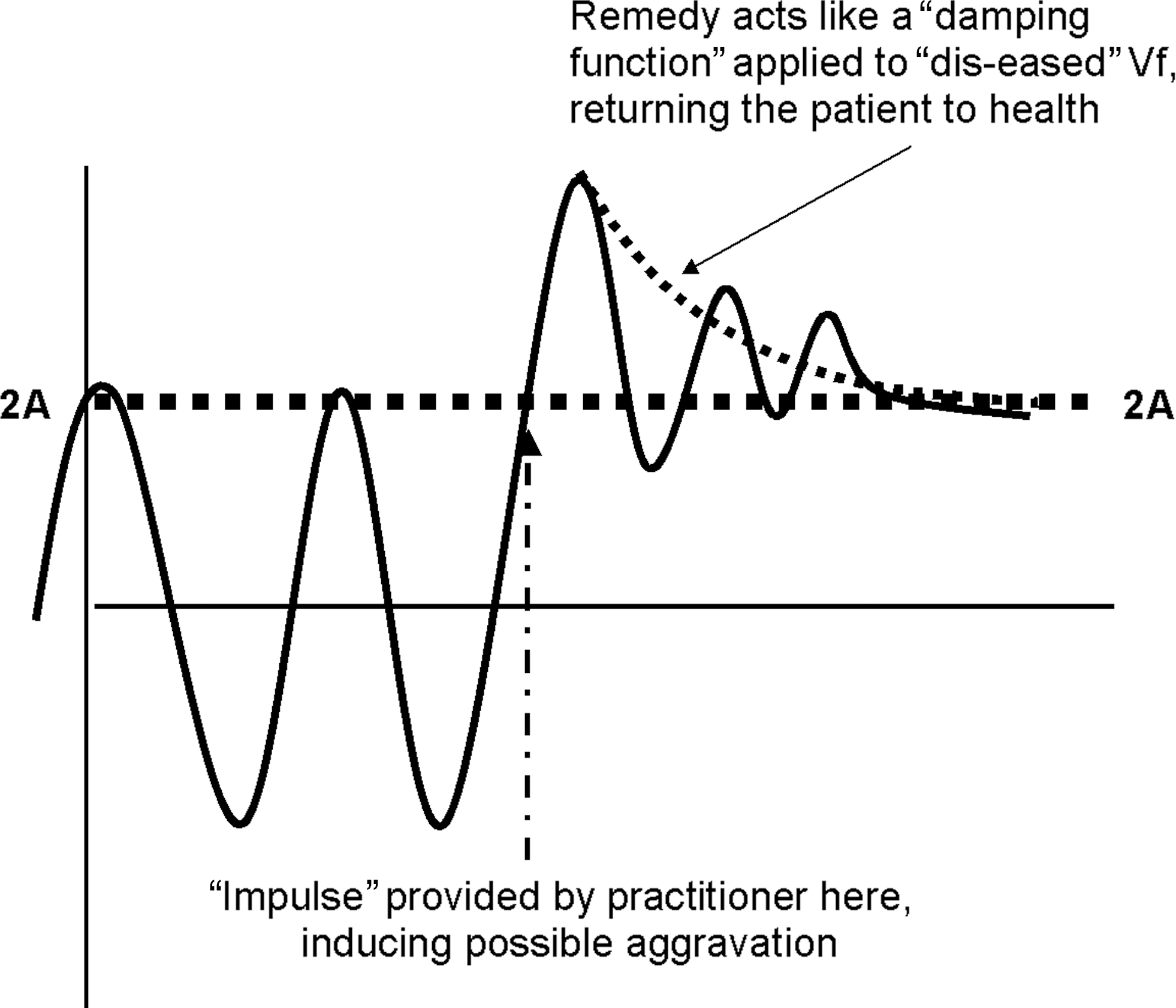
The combined effect of this “impulse” from the practitioner and curative remedy(s) can be crudely represented (Fig. 3) as bringing about a temporary increase in the amplitude of the patient's fluctuating wave function (possibly equivalent to the temporary aggravation of symptoms that sometimes occurs during homeopathic treatment),⁵³ which is then “damped out”⁵⁴ by the remedy(s), bringing the patient back to a healthier, less fluctuating state (i.e., Ψ_Vf = 2A).

FIG. 3.

“Unwell” patient vital force (Vf) (Ψ_Vf = 2Acosk₂S₂) seen as a wave form^17,20
–22 that increases in amplitude during generalized quantum entanglement between patient Px, practitioner Pr, and remedy Rx, via an “impulse” from the practitioner, and is then “damped” back⁵³ to its healthy state (Ψ_Vf = 2A) as a result of remedy action. The wave form is an expression of the degree of “unwellness” represented by the precessing axis of a quantized gyroscope oscillating around a fixed point: remedy and practitioner action “damp” this precession back so that the Vf stands upright, as opposed to falling over stopped (i.e., dead).

By considering the PPR entangled state semiotically to have the symmetry of a chiral tetrahedron (this arises from a previous treatment of the PPR entangled state),¹⁹ the practitioner may be considered to elaborate a “mirror-like” therapeutic state space in which this PPR entangled state is not only reflected, but also “inverted.” This means the therapeutic state space may be imagined as essentially two-dimensional (allowing the integration range of normalization to be over what is essentially a mirror plane; 0 to 2π).¹⁹ However, this therapeutic “mirror plane” is no simple passive reflector. By being able to “invert” that which is reflected in it (i.e., reflect back to the patient what a cured state might be), the therapeutic mirror plane may be thought to exhibit topologically the symmetry properties of a Möbius strip. Thus, by initially reflecting back the patient's dis-eased state, this may then be imagined, topologically speaking, as taking one “turn” around the therapeutic state space's Möbius strip, becoming inverted in the process into the practitioner's reflection of the cured state. This, the patient recognizes and moves toward (“ through the looking glass … ”), completing the representative stellated octahedron of the curative PPR entangled state.¹⁹ Throughout the therapeutic process, therefore, the value of A will fluctuate, gradually becoming smaller as the patient moves toward health.

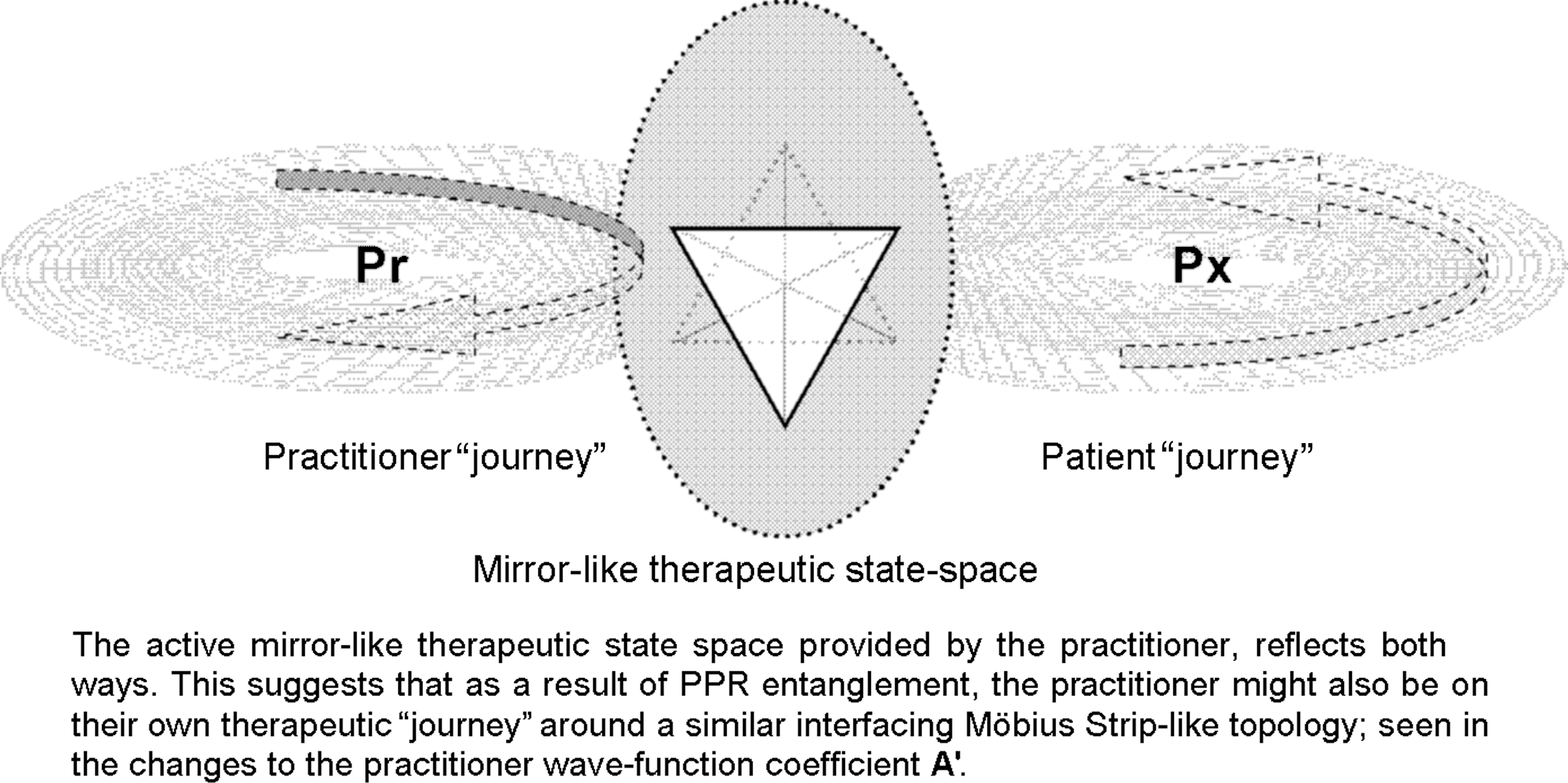
But what of the practitioner? How might the practitioner be affected or benefit in some way from PPR entanglement during the therapeutic process (Box 4)? A practitioner may well see many patients in a day, and it would be at the very least impractical to remain entangled with an entire day's clinic, who may not be seen again for a month. There will also be stress on the practitioner picked up from the patient. One could posit that perhaps any realistic long-term PPR entanglement might be through the “witnessing” effect of the remedy, but entanglement as mentioned here really refers to the set of (isolating from the outside world?) circumstances that occur during the consultation. It is here that the “therapeutic state space” is generated and maintained. Under these circumstance, the therapeutic “mirror” plane could be thought to reflect in both directions (Fig. 4A), and it is quite possible to perform a series of normalization operations similar to those in Boxes 1 and 2 that demonstrate how the practitioner wave function normalization constant A' might fluctuate through the therapeutic process (Box 4).

FIG. 4.

Entangled therapeutic “journeys” of patient and practitioner, as can be seen if one views the well-known Escher's “Drawing Hands” as an illustration. PPR, generalized quantum entanglement between patient Px, practitioner Pr, and remedy Rx. From Ref. 56.

Box 4. The Practitioner in the Therapeutic Process

The practitioner wave function was likened to a Kronecker or Dirac Δ function,²³ for providing an “impulse” to the patient, but this is from the patient's point of view only. The practitioner too is human, which means it should also be possible to view PPR entanglement from the practitioner's perspective: the “mirror” representing the therapeutic state space “reflects” in both directions. From this perspective, the practitioner wave function should be similar in form to the patient's, which because of the patient–practitioner relationship, would depend on the same set of patient secondary symptoms (S₂). Thus, “mirroring” the patient wave function' could mean the practitioner is to some extent susceptible to changes in the patient's state as the latter improves (which may coincide with transference and countertransference phenomena observed in a wide variety of therapies),⁵⁴ inferring that to some extent the patient and practitioner healing journeys interface with and affect each other.

Thus, wave functions representing two such possible practitioner states (e.g., more susceptible and less susceptible, respectively) during the therapeutic process might be \documentclass{aastex}\usepackage{amsbsy}\usepackage{amsfonts}\usepackage{amssymb}\usepackage{bm}\usepackage{mathrsfs}\usepackage{pifont}\usepackage{stmaryrd}\usepackage{textcomp}\usepackage{portland,xspace}\usepackage{amsmath,amsxtra}\pagestyle{empty}\DeclareMathSizes{10}{9}{7}{6} \begin{document} \begin{align*} \Psi_{{\rm Pr} \uparrow} = 2{\rm A}^{ \prime}{\rm cosk}^{ \prime}_2{\rm S}_2 \ {\rm and} \ \Psi_{{\rm Pr} \downarrow} = 2{\rm A}^{ \prime} \end{align*} \end{document}

where the constants A' and k'₂ have similar meanings to those for the patient wave function.^17,20
–22 Meanwhile, just as in patient-centered PPR entanglement where the practitioner is likened to a Δ function providing an “impulse” for the patient, so in this case, the patient may be thought to provide an “impulse” for the practitioner (i.e., Ψ_Px↑ = 1 and Ψ_Px↓ = 0 for a “well” and “unwell” patient, respectively).

The PPR entangled states given in equations (4 –7) (Box 1) may be normalized as they were in in in Box 2, and values for the constant A' in the practitioner's Vf wave function derived. Normalizing equation (4), for example, gives (11): \documentclass{aastex}\usepackage{amsbsy}\usepackage{amsfonts}\usepackage{amssymb}\usepackage{bm}\usepackage{mathrsfs}\usepackage{pifont}\usepackage{stmaryrd}\usepackage{textcomp}\usepackage{portland,xspace}\usepackage{amsmath,amsxtra}\pagestyle{empty}\DeclareMathSizes{10}{9}{7}{6} \begin{document} \begin{align*}<\Psi_{\rm PPR} \mid \Psi_{\rm PPR} > &= 1 / {2} [ (< \Psi_{{ \rm Px} \uparrow} \cdot \Psi_{{\rm Pr} \uparrow} \cdot \Psi_{{ \rm Rx} \uparrow}\mid \Psi_{{\rm Px} \uparrow} \cdot \Psi_{{\rm Pr} \uparrow} \cdot \Psi_{{\rm Rx} \uparrow} >)\ \pm\ (< \Psi_{{\rm Px} \uparrow} \cdot \Psi_{{\rm Pr} \uparrow} \cdot \Psi_{{\rm Rx} \uparrow}\mid \Psi_{{\rm Px} \downarrow} \cdot \Psi_{{\rm Pr} \downarrow} \cdot \Psi_{{\rm Rx} \downarrow} >)\ \\&\quad\pm\ (< \Psi_{{\rm Px} \downarrow} \cdot \Psi_{{\rm Pr} \downarrow} \cdot \Psi_{{\rm Rx} \downarrow}\mid \Psi_{{\rm Px} \downarrow} \cdot \Psi_{{\rm Pr} \downarrow} \cdot \Psi_{{\rm Rx} \downarrow} >)\ \pm\ (< \Psi_{{\rm Px} \downarrow} \cdot \Psi_{{\rm Pr} \downarrow} \cdot \Psi_{{\rm Rx} \downarrow}\mid \Psi_{{\rm Px} \uparrow} \cdot \Psi_{{\rm Pr} \uparrow} \cdot \Psi_{{\rm Rx} \uparrow} >) ]\ =\ 1 \tag {11} \end{align*} \end{document}

Similar equations can be written using (5 –7). Inspecting these as before (and remembering it is now Ψ_Px↑ = 1 and Ψ_Px↓ = 0), three of the terms in each of the normalization equations will cancel out. However, it is the patient, not the practitioner, for whom the case is taken and the remedy prescribed. So as far as the practitioner is concerned, PPR entanglement results in either the patient's symptoms being removed or not; therefore, for the practitioner we only need to consider the cases of when symptoms are removed S₂ → 0, and postentanglement superposition (i.e., steps 2 and 3 [Box 2], and Fig. 1).

Step 2 : “Let the dog see the rabbit … .”: Removing the symptoms S₂ → 0.

Considering the PPR entangled state from equation (4), and substituting Ψ_Pr↑ = 2A'; Ψ_Px↑ = 1; Ψ_Rx↑ = 1; Ψ_Pr↓ = 2A'cosk₂'S₂; Ψ_Px↓ = 0, and Ψ_Rx↓ = e^-ik₂ ^ΔS₂ (and their complex conjugates) into equation (11) gives: \documentclass{aastex}\usepackage{amsbsy}\usepackage{amsfonts}\usepackage{amssymb}\usepackage{bm}\usepackage{mathrsfs}\usepackage{pifont}\usepackage{stmaryrd}\usepackage{textcomp}\usepackage{portland,xspace}\usepackage{amsmath,amsxtra}\pagestyle{empty}\DeclareMathSizes{10}{9}{7}{6} \begin{document} \begin{align*}< \Psi_{\rm PPR} \mid \Psi_{\rm PPR} > = 1 / 2 \int ( \{ { 2\rm A}^{ \prime} \cdot {\rm e}^{i{\rm k}_2 ^{\prime} {\rm S}_{2.1}} \cdot {\rm e}^{i{\rm k}_2^{\prime} {\rm S}_2}\} \{ {2{\rm A}^{ \prime} \cdot {\rm e}^{ - i{\rm k}_2^{\prime} {\rm S}_{2.1}}} \cdot {\rm e}^{ - i{\rm k}_2^{\prime} {\rm S_2}} \}) {\rm dS}_2= 1 \end{align*} \end{document} \documentclass{aastex}\usepackage{amsbsy}\usepackage{amsfonts}\usepackage{amssymb}\usepackage{bm}\usepackage{mathrsfs}\usepackage{pifont}\usepackage{stmaryrd}\usepackage{textcomp}\usepackage{portland,xspace}\usepackage{amsmath,amsxtra}\pagestyle{empty}\DeclareMathSizes{10}{9}{7}{6} \begin{document} \begin{align*}< \Psi_{\rm PPR} \mid \Psi_{\rm PPR} > = 1 / 2 \int ( \{ 2{\rm A}^{ \prime} \cdot 1.1 \} \{ 2{\rm A}^{ \prime} \cdot 1.1 \}){\rm dS}_{2} = 1 \end{align*} \end{document}

And again integrating between 0 to 2π gives \documentclass{aastex}\usepackage{amsbsy}\usepackage{amsfonts}\usepackage{amssymb}\usepackage{bm}\usepackage{mathrsfs}\usepackage{pifont}\usepackage{stmaryrd}\usepackage{textcomp}\usepackage{portland,xspace}\usepackage{amsmath,amsxtra}\pagestyle{empty}\DeclareMathSizes{10}{9}{7}{6} \begin{document} \begin{align*} 1 / {2} \int 4{\rm A}^{ \prime 2} \cdot {\rm dS}_{2} = [ 2{\rm A}^{\prime 2} \cdot {\rm S}_2 ] = 1 \cdot [ 2{\rm A}^{ \prime 2} \cdot 2 \pi ] = 1 , \quad{\rm and} \ \underline{{\rm A}^{ \prime} = 1 / {2 \sqrt \pi} \approx 0.282}. \end{align*} \end{document}

Inspecting equation (5) and normalizing as in equation (11) delivers the same result; \documentclass{aastex}\usepackage{amsbsy}\usepackage{amsfonts}\usepackage{amssymb}\usepackage{bm}\usepackage{mathrsfs}\usepackage{pifont}\usepackage{stmaryrd}\usepackage{textcomp}\usepackage{portland,xspace}\usepackage{amsmath,amsxtra}\pagestyle{empty}\DeclareMathSizes{10}{9}{7}{6}\begin{document}$${\rm A}^{\prime} = 1 / {2 \sqrt \pi}$$\end{document} . However, similar inspection of equations (6) and (7) and then normalization via equation (11), gives \documentclass{aastex}\usepackage{amsbsy}\usepackage{amsfonts}\usepackage{amssymb}\usepackage{bm}\usepackage{mathrsfs}\usepackage{pifont}\usepackage{stmaryrd}\usepackage{textcomp}\usepackage{portland,xspace}\usepackage{amsmath,amsxtra}\pagestyle{empty}\DeclareMathSizes{10}{9}{7}{6}\begin{document}$${\rm A}^{\prime} = 1 /{\sqrt 2 \pi}$$\end{document} , as in step 1 above. In (4) and (5), the patient and the practitioner are both up arrowed (i.e., entangled “in synch” with each other), so that \documentclass{aastex}\usepackage{amsbsy}\usepackage{amsfonts}\usepackage{amssymb}\usepackage{bm}\usepackage{mathrsfs}\usepackage{pifont}\usepackage{stmaryrd}\usepackage{textcomp}\usepackage{portland,xspace}\usepackage{amsmath,amsxtra}\pagestyle{empty}\DeclareMathSizes{10}{9}{7}{6}\begin{document}$${\rm A}^{ \prime} = 1 / {2 \sqrt \pi} \approx 0.282$$\end{document} , while in (6) and (7) the patient and practitioner are alternately up and down-arrowed, i.e., entangled “out of synch” with each other and give \documentclass{aastex}\usepackage{amsbsy}\usepackage{amsfonts}\usepackage{amssymb}\usepackage{bm}\usepackage{mathrsfs}\usepackage{pifont}\usepackage{stmaryrd}\usepackage{textcomp}\usepackage{portland,xspace}\usepackage{amsmath,amsxtra}\pagestyle{empty}\DeclareMathSizes{10}{9}{7}{6}\begin{document}$${\rm A}^{ \prime} = 1 / {\sqrt 2 \pi} \approx 0.4$$\end{document} .

Step 3 : “Through the looking glass … .”: Postentanglement self-superposition

After PPR entanglement, self-superposition⁴⁷ of the patient's well and unwell states leads to a further reduction in the value of A on normalization. This could be represented as: \documentclass{aastex}\usepackage{amsbsy}\usepackage{amsfonts}\usepackage{amssymb}\usepackage{bm}\usepackage{mathrsfs}\usepackage{pifont}\usepackage{stmaryrd}\usepackage{textcomp}\usepackage{portland,xspace}\usepackage{amsmath,amsxtra}\pagestyle{empty}\DeclareMathSizes{10}{9}{7}{6} \begin{document} \begin{align*} \mid \Psi_{\rm Pr} > = 1 / {\sqrt 2} (\mid \Psi_{{\rm Pr} \uparrow} > \ \pm \ \mid \Psi_{{\rm Pr} \downarrow} >) \tag {12} \end{align*} \end{document} \documentclass{aastex}\usepackage{amsbsy}\usepackage{amsfonts}\usepackage{amssymb}\usepackage{bm}\usepackage{mathrsfs}\usepackage{pifont}\usepackage{stmaryrd}\usepackage{textcomp}\usepackage{portland,xspace}\usepackage{amsmath,amsxtra}\pagestyle{empty}\DeclareMathSizes{10}{9}{7}{6} \begin{document} \begin{align*}{\rm And} &<\Psi_{\rm Pr} \mid \Psi_{\rm Pr} > 1 / 2 (< \Psi_{{\rm Pr} \uparrow}\mid \pm \ < \Psi_{{\rm Pr} \downarrow}\mid) (\mid \Psi_{{\rm Pr} \uparrow} > \pm \ \mid \Psi_{{\rm Pr} \downarrow} >) = 1 / 2 (< \Psi_{{\rm Pr} \uparrow}\mid \Psi_{{\rm Pr} \uparrow} > \ \pm \ < \Psi_{{\rm Pr} \uparrow}\mid \Psi_{{\rm Pr} \downarrow} > \\\pm &< \Psi_{{ \rm Pr} \downarrow}\mid \Psi_{{\rm Pr} \downarrow} > \pm < \Psi_{{\rm Pr} \downarrow}\mid \Psi_{{\rm Pr} \uparrow} >) = 1 \end{align*} \end{document}

“Well” practitioner is |Ψ_Pr↑ > = 2A'; “unwell” practitioner Ψ_Pr↓ = 2A'cosk₂'S₂: so, substituting normalizing and integrating: \documentclass{aastex}\usepackage{amsbsy}\usepackage{amsfonts}\usepackage{amssymb}\usepackage{bm}\usepackage{mathrsfs}\usepackage{pifont}\usepackage{stmaryrd}\usepackage{textcomp}\usepackage{portland,xspace}\usepackage{amsmath,amsxtra}\pagestyle{empty}\DeclareMathSizes{10}{9}{7}{6} \begin{document} \begin{align*}< \Psi_{\rm Pr} \mid \Psi_{\rm Pr} > = 1 / 2 \int 4{\rm A}^{ \prime ^2} (1 \ \pm \ 2{\rm cosk}_{2^\prime}{\rm S}_2 + \cos^2{ \rm k}_{2^\prime}{\rm S}_2) \cdot {\rm dS}_2 = 2{\rm A} ^{\prime 2} [ {\rm S}_2 \pm 2 / {\rm k}_{2 ^\prime}{\rm sink}_{2^ \prime}{\rm S}_2 + {\rm S}_2 / 2 ] = 1 \ {\rm \quad and} \ \underline{{\rm A}^{ \prime} = 1 / {\sqrt 6 \pi}} \end{align*} \end{document}

It might appear from this analysis that changes in the practitioner's A' values inversely track precisely those of the patient's A. The point here is that the practitioner and patient wave functions have different energies, represented by different k₂ values (i.e., k₂' and k₂, respectively) so that even though A' and A might track each other, it does not mean energetically their individual wave functions do so.

Here, of course, the patient could be said to be acting as an “impulse” function for the practitioner.⁴⁷ These fluctuations in A' (Fig. 1, gray bars and arrows) during therapeutic entanglement seem to be the inverse of those of the patient's A, in that where A is decreasing, A' is increasing; in other words, the state of the practitioner's Vf wave function might be inversely affected by changes occurring to the patients during the therapeutic process (Fig. 4A). Thus, though as drawn in Figure 1, fluctuations in A' for the practitioner seem to inversely track A for the patient during entanglement, the point here is that the practitioner and patient wave functions have different energies, represented by different k₂ values (i.e., k₂' and k₂, respectively). Consequently, even though A' and A might inversely track each other, it does not necessarily mean that energetically their individual wave-functions do so. Figure 1, therefore, is only a crude representation of how the Vf's of patient and practitioner might interact, and could have some bearing on the understanding of expectation in the therapeutic process, and transference/countertransference phenomena believed to operate in patient–practitioner interactions in a variety of therapeutic modalities.⁵⁵

Alternatively, the way A and A' exchange, as suggested within the gray area in Figure 1, may be an expression of the way that the patient's healing journey interfaces with and affects the practitioner's own, and vice versa. Ultimately, during the journey to cure, both A and A' return to lower values. This possible interplay between the patient and the practitioner is rather aptly represented in the etching by M.C. Escher of “Drawing Hands” (Fig. 4B).^56,57

Conclusions

In conclusion, this article has tried to show what could happen when two previous nonorthodox quantum metaphor/models of the homeopathic therapeutic process are combined. It allows via “normalization” of the Vf “gyroscopic” wave function Ψ_Vf = 2Acosk₂S₂, values of the constant A to be assessed that, in turn, permit topological insights into the practitioner-derived therapeutic state space, and the patient's journey to cure.

Footnotes

Acknowledgments

In preparing the manuscript, the author wishes to gratefully acknowledge the invaluable assistance of Alex Hankey, PhD; Caroline Diederichs, PhD; David Hefferon, BDS, DipHomtox (Hons), AIAOMT; and Ms. Niki Fforde. This article is dedicated to the memory of the late M. Jean-Claude Fouquin and his family.

Disclosure Statement

No competing financial interests exist.

*

By overconcentrating on science's perceived implied separation of epistemological and political/moral/ethical issues, postmodern critiques of science have themselves been heavily criticized for signally failing to comprehend the universality of its empirical claims and terminology. Nevertheless, a postmodern deconstruction of evidence-based medicine has successfully pointed out its increasing intolerance of therapeutic pluralism in health care systems.

References

Baum

, Ernst

. Should we maintain an open mind about homeopathy? Am J Med, 2009; 122:973–974.

Chaplin

. Water Structure and Behaviour. www.lsbu.ac.uk/water/. 2008 October 19.

van Wijk

, Albrecht

. Proving and therapeutic experiments in the HonmBRex basic homeopathy research database. Homeopathy, 2007; 96:252–257.

Shang

, Huwiler-Müntener

, Nartey

et al. Are the clinical effects of homoeopathy placebo effects? Comparative study of placebo-controlled trials of homoeopathy and allopathy. Lancet, 2005; 366:726–732.

Lüdtke

, Rutten

ALB

. The conclusions on the effectiveness of homeopathy highly depend on the set of analyzed trials. J Clin Epidemiol, 2008; 61:1179–1204.

Rutten

ALB

, Stolper

. The 2005 meta-analysis of homeopathy: The importance of post-publication data. Homeopathy, 2008; 97:169–177.

Kirsch

, Deacon

, Huendo-Medina

et al. Initial severity and antidepressant benefits: A meta-analysis of data submitted to the Food and Drug Administration. PloS Med, 2008; 5:e45.

Milgrom

. Treating Leick with like: Response to criticisms of the use of entanglement to illustrate homeopathy. Homeopathy, 2008; 97:96–99.

Zeilinger

. Quantum Teleportation and the Nature of Reality. 2004. www.btgjapan.org/catalysts/anton.html. 2008 March 21.

10.

d'Espagnet

. On Physics and Philosophy. Princeton, NJ: Princeton University Press, 2006.

11.

Scully

, Zubairy

, Agarwal

, Walther

. Extracting work from a single heat bath via vanishing quantum coherence. Science, 2003; 299:862–864.

12.

Walach

. Generalised entanglement: A new theoretical model for understanding the effects of complementary and alternative medicine. J Altern Complement Med, 2005; 11:549–559.

13.

Atmanspacher

, Römer

, Walach

. Weak quantum theory: Complementarity and entanglement in physics and beyond. Found Phys, 2002; 32:379–406.

14.

Sokal

, Briemont

. Intellectual Impostures. London: Profile Books Ltd., 1998.

15.

Holmes

, Murray

, Perron

, Rail

. Deconstructing the evidence-based discourse in health sciences: Truth, power, and fascism. Int J Evid Based Healthc, 2006; 4:180.

16.

Copenhauer

. Hermetica. Cambridge, UK: Cambridge University Press, 1992.

17.

Wichmann

. Defining a different tradition for homeopathy. Homeopathic links, 2001; 14:202–203.

18.

Milgrom

. Patient-practitioner-remedy (PPR) entanglement, Part 9: “Torque”-like action of the homeopathic remedy. J Altern Complement Med, 2006; 12:915–929.

19.

Milgrom

. A new geometrical description of entanglement and the curative homeopathic process. J Altern Complement Med, 2008; 14:329and references therein.

20.

Sherr

. The Dynamics and Methodology of Homeopathic Provings. West Malvern, UK: Dynamis Books, 1994.

21.

Dirac

PAM

. The Principles of Quantum Mechanics, 4th. Oxford, UK: Oxford University Press, 1982; 18ff.

22.

Milgrom

. Patient-practitioner-remedy (PPR) entanglement, Part 7: A gyroscopic metaphor for the vital force and its use to illustrate some of the empirical laws of homeopathy. Forsch Komplementärmed, 2004; 11:212.

23.

Milgrom

. Patient-practitioner-remedy (PPR) entanglement, Part 10: Toward a unified theory of homeopathy and conventional medicine. J Altern Complement Med, 2007; 13:759–770.

24.

Coulter

. Homeopathic Science and Modern Medicine: The Physics of Healing with Microdoses. Berkeley: North Atlantic Books, 1981.

25.

Milgrom

. Patient–practitioner–remedy (PPR) entanglement: Part 8. “Laser-like” action of the homeopathic therapeutic encounter as predicted by a gyroscopic metaphor for the vital force. Forsch Komplementärmed Klass Naturheilkd, 2005; 12:206–313.

26.

Walach

. Homeopathy as semiotic. Semiotica, 1991; 83:81–85.

27.

Walach

. Magic of signs. Br Hom J, 2000; 89:127–140.

28.

Gernert

. Towards a closed description of observation processes. BioSystems, 2000; 54:165–180.

29.

Gernert

. Conditions for entanglement. Front Perspect, 2005; 14:8–13.

30.

Milgrom

. Patient–practitioner–remedy (PPR) entanglement: Part 1. A qualitative non-local metaphor for homeopathy based on quantum theory. Homeopathy, 2002; 91:239–248.

31.

Nadeau

, Kafatos

. The Non-local Universe: The New Physics and Matters of the Mind. Oxford, UK and New York: Oxford University Press, 1999.

32.

Weingärtner

. An approach to the scientific identification of a therapeutically active ingredient of high potencies. Forsch Komplementarmed Klass Naturheilkd, 2002; 9:229–233.

33.

Weingärtner

. The nature of the active ingredient in ultramolecular dilutions. Homeopathy, 2007; 96:220–226.

34.

Walach

. Entanglement model of homeopathy as an example of generalised entanglement predicted by weak quantum theory. Forsch Komplementärmed Klass Naturheilkd, 2003; 10:192–200.

35.

Hyland

. Does a form of “entanglement” between people explain healing? An examination of hypotheses and methodology. Complement Ther Med, 2004; 12:198–208.

36.

Milgrom

. Patient–practitioner–remedy (PPR) entanglement: Part 3. Refining the quantum metaphor for homeopathy. Homeopathy, 2003; 92:152–160.

37.

Milgrom

. Patient–practitioner–remedy (PPR) entanglement: Part 4. Towards classification and unification of the different entanglement models for homeopathy. Homeopathy, 2004; 93:34–42.

38.

Greenberger

, Horne

, Shimony

, Zeilinger

. Bell's theorem without inequalities. Am J Phys, 1990; 58:1131–1143.

39.

Milgrom

. Journeys in the country of the blind: Entanglement theory and the effects of blinding on trials of homeopathy and homeopathic provings. eCAM, 2007; 4:7.

40.

Möllinger

, Schneider

, Löffel

et al. A double blind randomized homeopathic pathogenic trial with healthy persons: Comparing two high potencies. Forsche Komplementarmed, 2004; 11:274–280.

41.

Walach

, Sherr

, Schneider

et al. Homeopathic proving symptoms: Result of a local, non-local, or placebo process? A blinded, placebo-controlled pilot study. Homeopathy, 2004; 93:179–185.

42.

Dominici

, Bellavite

, di Stanislao

et al. Double-blind placebo-controlled homeopathic pathogenic trials: Symptom collection and analysis. Homeopathy, 2006; 95:123–130.

43.

Walach

, Mollinger

, Sherr

, Schneider

. Homeopathic pathogenic trials produce more specific than non-specific symptoms: Results from two double-blind placebo controlled trials. J Psychopharmacol, 2008; 22:543.

44.

Milgrom

. Patient–practitioner–remedy (PPR) entanglement: Part 6. Miasms revisited: Non-linear quantum theory as a model for the homeopathic process. Homeopathy, 2004; 93:154–158.

45.

Spiegel

. Schaum's Outline of Theory and Problems of Complex Variables. New York: McGraw-Hill, 1999.

46.

Normalization. http://cat.middlebury.edu/∼chem/chemistry/class/physical/quantum/help/normalize/normalize.html. 2009 November 15.

47.

Weisstein

. “Delta Function.” From MathWorld—A Wolfram Web Resource. http://mathworld.wolfram.com/DeltaFunction.html. 2009 November 15.

48.

Masahito

. Quantum Information: An Introduction. Berlin, Heidelberg: Springer-Verlag, 2006.

49.

Aravind

. The “twirl,” stella octangula, and mixed state entanglement. Phys Lett A, 1997; 233:7–10.

50.

Pickover

. The Möbius Strip: Dr August Möbius's Marvellous Band in Mathematics, Games, Literature, Art, Technology, and Cosmology. New York: Thunder's Mouth Press, Avalon Publishing Group, 2006.

51.

Hollas

. Modern Spectroscopy, 3rd. Chichester, UK: John Wiley and Sons, 1996.

52.

Gribbin

. Q is for Quantum. London: Phoenix Press, 2002.

53.

Vithoulkas

. The Science of Homeopathy. New York: Grove Press, 1980.

54.

Weisstein

. “Damped Simple Harmonic Motion—Critical Damping.” From MathWorld—A Wolfram Web Resource. http://mathworld.wolfram.com/DampedSimpleHarmonicMotionCriticalDamping.html. 2009 November 15.

55.

Withers

. Psychoanalysis, Complementary Medicine, and the Placebo. Peters

. Understanding the Placebo Effect in Complementary Medicine: Theory, Practice, and Research. London: Churchill-Livingstone, 2001; 111–129.

56.

Escher

. Drawing Hands. 1948. http://www.google.co.uk/search?sourceid=navclient&aq=0h&oq=drawing&hl=en-GB&ie=UTF-8&rlz=1T4TSED_en-GBGB304GB305&q=drawing+hands+escher. 2009 November 15.

57.

Goswami

. The Self-Aware Universe: How Consciousness Creates The Material World. New York: Jeremy P. Tarcher/Putnam, 1995.

Toward a Topological Description of the Therapeutic Process

Abstract

Introduction:

Method:

Results:

Conclusions:

Introduction

PPR Entanglement Models Revisited (Box 1) 20 –23

Box 1. Defining Wave Functions for PPR Entanglement

Gyroscopic model 18

PPR entanglement model 19

Normalization of the Patient's Vf Wave Function (Box 2) 45

Box 2. Normalization and the Patient Vf Wave Function

Normalization in the therapeutic context

Normalization of the patient Vf wave function

Box 3. Changing Values for the Constant A on Normalization

Discussion

Box 4. The Practitioner in the Therapeutic Process

Conclusions

Footnotes

Acknowledgments

Disclosure Statement

*

References

PPR Entanglement Models Revisited (Box 1)^20

–23

Gyroscopic model¹⁸

PPR entanglement model¹⁹

Normalization of the Patient's Vf Wave Function (Box 2)⁴⁵