Adjusting the Fitting of Fluorescence-Based Dose–Response Kinase Inhibition Assay to Account for Fluorescent Inhibitors

Abstract

Fluorescence is routinely used to monitor kinase inhibition in commercial assays. Occasionally fluorescent compounds can interfere with the fluorescent reading. To address this issue, the problematic data are usually truncated to improve the fit, however, this approach raises ethical and reproducibility concerns. Instead, it is suggested to adjust the fitting formula, to account for the autofluorescence of the compounds and improve the fit of the data compared with a naive approach. Finally, it was noticed that truncating the data can result in a small underestimation of the IC₅₀ values and should therefore be used carefully.

INTRODUCTION

Since the early 2000s, kinase inhibition has been regarded as a successful strategy to tackle cancers inter alia, resulting in over 100 such drugs approved by different organizations by 2023. The majority of kinase inhibitors are small molecules (small-molecule kinase inhibitors, SMKI)^1,2 and in parallel to their development, assays to measure kinase inhibition have also appeared and improved rapidly.³ A popular option to test a potential kinase inhibitor is time-resolved fluorescence resonance energy transfer (TR-FRET) that assesses binding of compounds to kinase active sites.^4,5 In these assays, the kinase of interest is labeled with lanthanide tagged antibodies, with affinity for the kinase purification tag, while tracers linked to fluorophores bind the kinase active site (Fig. 1A). The TR-FRET signal between the antibody and the tracer is then monitored with a fluorescence plate reader.

Fig. 1.

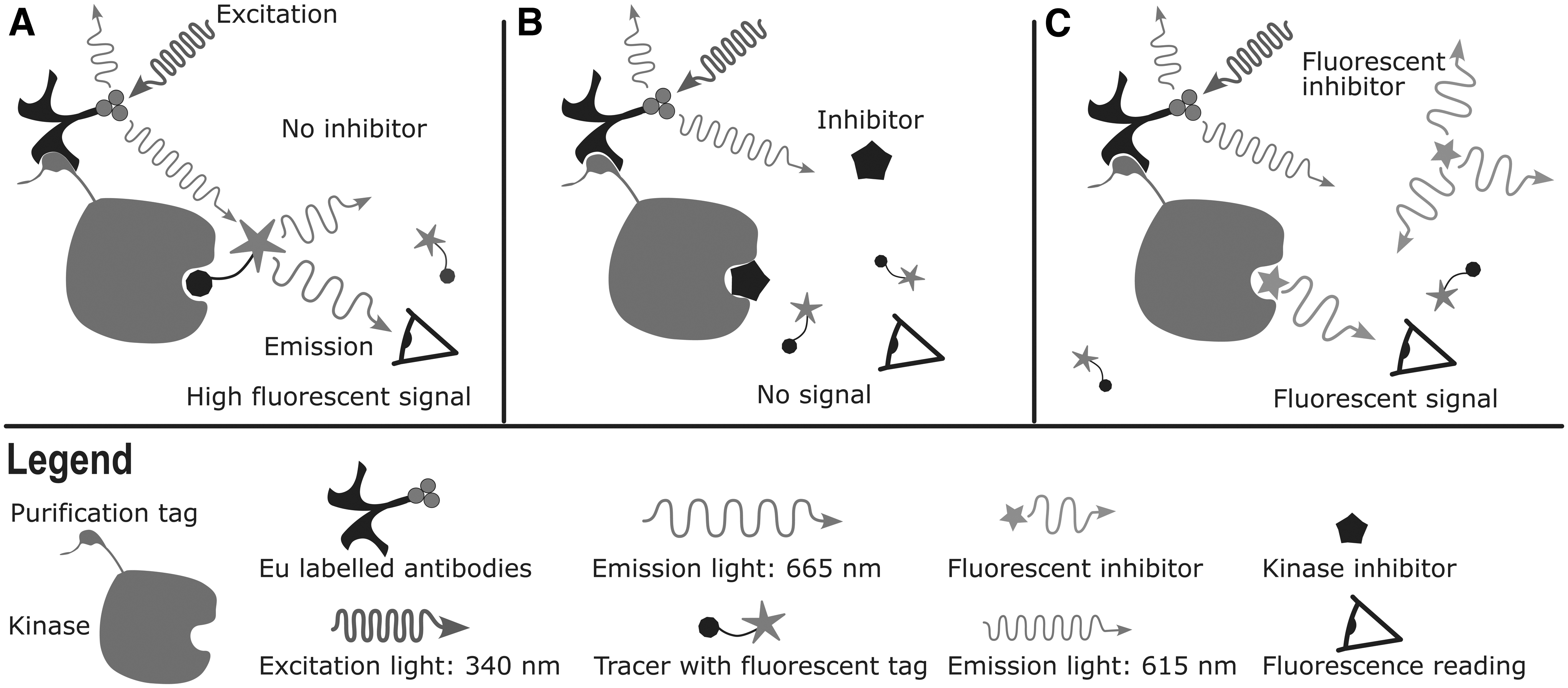
Graphical summary of TR-FRET kinase binding assay. (A) A system made of europium-labeled antibody, kinase, and fluorescent tracer, relays a signal that can be monitored at wavelength 665 nm with a fluorescent plate reader. (B) When adding inhibitor to the system, the tracer has to compete with the inhibitor for the kinase active site and the signal intensity is reduced proportionally to the binding of the inhibitor to the kinase. (C) Occasionally the inhibitor itself can be fluorescent, in which case the signal may increase proportionally to the inhibitor concentration in addition to the fluorescence resulting from the europium-tracer relay. TR-FRET, time-resolved fluorescence resonance energy transfer.

In a typical experiment, the tracer must compete with the SMKIs for the adenosine triphosphate binding pocket, which leads to a reduction of the TR-FRET signal based on the affinity and concentration of the SMKIs (Fig. 1B). Finally, the measured fluorescent signal intensity is plotted against the compound concentration and these values are fitted with Eq. (1) to determine the IC₅₀ values of each SMKI. $Y = b o t + \frac{(t o p - b o t)}{1 + {10^{(X - K)}}^{}}$ (1)

Where Y is the fluorescent intensity, X the Log₁₀ of the compound concentration, and K is the Log₁₀(IC₅₀).

Eq. (1) can be derived from the Hill equation,⁶ which despite its simplicity is still in use today (also described as “Hill–Langmuir equation”).⁷ Eq. (1) reports on the complex formation indirectly hence allowing for parameters such as bot and top, which account for the background signal and signal amplitude. In addition, Eq. (1) takes concentrations in a logarithmic scale, which is practical for experimental setups where compounds are prepared through dilution series. However, experiments are usually imperfect, and the measured fluorescent signal Y describes more than the fraction of complex formed. Any contribution to the fluorescence is included in Y, including phenomenon such as the autofluorescence of the components tested (Fig. 1C). When these external sources of fluorescence become dominant, the fitting of the data does not reliably represent the IC₅₀ values anymore and the model needs to be adjusted.

The current recommendation to treat data points that drift from the bot parameter, due to fluorescent compounds, for example, is to ignore these points. This approach allows for a quick and easy fix, which does improve the fitting and can sometimes help calculate IC₅₀ values even when the data suffer from drifting. However, removing data points arbitrarily raises reproducibility issues (are the removed data points always mentioned in the methods?) and ethical ones (where is the line between removing an outlier and removing points to make the data fit better to the initial hypothesis?). Here, I propose a simple adjustment to Eq. (1), to account for compound autofluorescence instead. This adjustment improves the results compared with a naive fit, without having to (arbitrarily) truncate the data either.

RESULTS

Treating the Autofluorescence of Compound as Linear

It was assumed that, at low species concentration, everything else being equal, the fluorescence of the species increases linearly with its concentration.⁸ This assumption does not apply to phenomena such as J-aggregation or other types of aggregation that might affect the fluorescence in a nonlinear manner.⁹ However, this assumption has the merit of simplicity and is consistent with the observation that the fluorescence of the compounds presented in this article increased linearly with their concentration in aqueous solution and in the absence of tracer or europium-tagged antibodies. Therefore, the autofluorescence of the compound was approximated with the equation: $Y = m \times L$ where Y represents the fluorescent reading value, L the concentration of the species, and m is a parameter that englobes all the other factors (large m corresponds to highly fluorescent compounds, whereas an m close to 0 means that the compound does not fluoresce).

After converting it to the logarithmic form, the linear equation was combined with Eq. (1), resulting in Eq. (2). $Y = b o t + \frac{(t o p - b o t)}{1 + {10^{(X - K)}}^{}} + m \times 1 0^{X}$ (2)

Where Y is the fluorescent reading, K is the Log₁₀(IC₅₀), X is the Log₁₀(Concentration), and top, bot, and m are parameters governed by the experimental setup.

Experimental Testing of Eq. (2)

Five data sets with varying signal amplitudes and signal-to-noise ratio were selected to test and assess Eq. (2). These data sets are representative of many situations encountered while performing LanthaScreen™ kinase binding assays. The raw data are available in Supplementary Material S1.

Data set 1 shows “good” data: high signal-to-noise ratio and little sign of autofluorescence.

In data sets 2 and 3, the signal is not as good, and the emission ratio (the emission ratio is proportional to the TR-FRET signal intensity) amplitude is much smaller, in these cases, the autofluorescence of the compound becomes noticeable, and there is no obvious plateau of the emission ratio at high compound concentration that can be described by the parameter bot. Data set 4 is an extreme such case; and the typical recommendation here is to truncate the last two to three data points to improve the fit. Finally, data set 5 comes from data with very small amplitude (kinases or antibodies are degraded), in this case the signal-to-noise ratio is small and the autofluorescence of the compound is distorting the results. These data should typically be reacquired if possible. To compare Eq. (2) with the current recommendation, the data sets were analyzed with three different approaches:

A naive fit approach, simply fitting the data with Eq. (1) without additional curation.

A truncated fit approach: upon inspection of the data, the points that deviate from the fit with Eq. (1) were removed and the truncated data were fitted once again with Eq. (1).

An adjusted fit approach: fitting the data as is, with an equation that accounts for the fluorescence of the compound Eq. (2) keeping all the data points in.

In data set 1, where the data are considered “good,” the results are the same regardless of the method used for the fitting (which is good! Table 1).

Table 1.

Fitting Good-Quality Data


Fit	IC₅₀ (nM)	Bot	Top	m	#Data	R ²
Naïve	105.2 (83.5–132.6)	0.0074 (0.0072–0.0077)	0.0137 (0.0134–0.0139)	—	36/36	0.985
Truncated	111.5 (88.5–140.5)	0.0073 (0.0071–0.0076)	0.0136 (0.0134–0.0138)	—	33/36	0.986
Adjusted	112.8 (87.3–145.6)	0.0073 (0.0070–0.0076)	0.0136 (0.0134–0.0139)	6.59e⁻⁹ (−4.038e⁻⁹ to 1.733e⁻⁸)	36/36	0.985

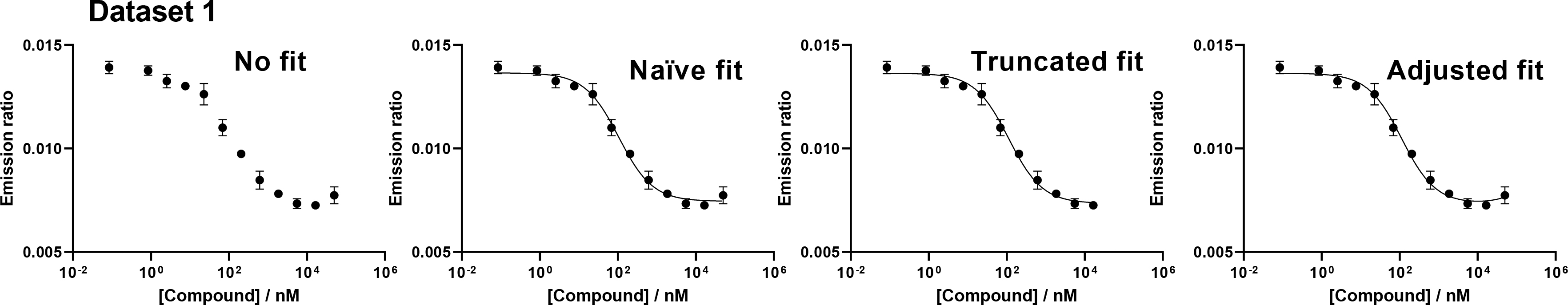
Top panel represents data set 1 fitted with the three different approaches: naive, truncated, and adjusted. The Y axis shows the emission ratio and the X-axis the compound concentration on a logarithmic scale. The bottom panel summarizes the parameters from the different fitting approaches, with the best fit value in bold and the 95% CI for the value given in parentheses. #Data represent the number of points used for the fit compared with the number of points available, R ² represents the nonlinear goodness of the fit using the different approaches.

CI, confidence interval.

In the second example presented, data sets 2 and 3, the deviation from a flat bot plateau, caused by the fluorescence of the compounds, is more marked than in data set 1. Obviously the “naive” approach should be avoided upon inspection of the data (Table 2).

Table 2.

Fitting Slightly Fluorescent Data


Fit	IC₅₀ (nM)	Bot	Top	m	#Data	R ²
Naive	179.8 (60.2–497.3)	0.0331 (0.0321–0.0340)	0.0373 (0.0376–0.0391)	—	36/36	0.710
Truncated	274.9 (156.5–476.1)	0.0318 (0.0312–0.0325)	0.0386 (0.0381–0.0391)	—	27/36	0.931
Adjusted	416.3 (190.2–895.0)	0.0310 (0.0297–0.0322)	0.0382 (0.0377– 0.0388)	4.74e⁻⁸ (2.846e⁻⁸ to 6.713e⁻⁸)	36/36	0.844


Fit	IC₅₀ (nM)	Bot	Top	m	#Data	R ²
Naive	311.6 (137.8–689.5)	0.0332 (0.0324–0.0339)	0.0379 (0.0374–0.0384)	—	36/36	0.779
Truncated	354.3 (180.0–694.9)	0.0325 (0.03167–0.03318)	0.0383 (0.0377–0.0390)	—	24/36	0.891
Adjusted	533.2 (262.7–1079)	0.0319 (0.0308–0.0329)	0.0379 (0.0374–0.0383)	2.90e⁻⁸ (1.315e⁻⁸ to 4.557e⁻⁸)	36/36	0.847

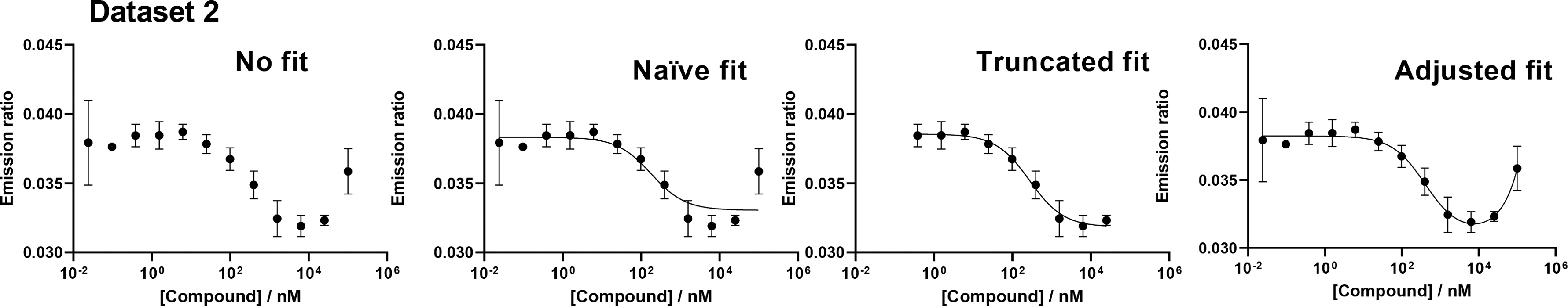
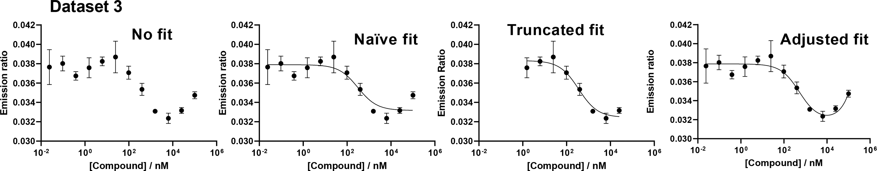
For the truncated fit approach, outliers both at high compound concentration and noisy data at low compound concentration were removed (for a total of 12 points removed in data set 2 and 15 points in data set 3). In this example, the naive fit gives poor results, underestimating the IC₅₀ values as the measured fluorescence of points at high compound concentration is increasing again. Unsurprisingly, R ² values are also worse for the naive fit approaches. The R ² values for the adjusted fit are not as good as that of the truncated fit, but mainly because of keeping the points with high standard deviation at a low compound concentration. The 95% CI for the IC₅₀ value is larger for the adjusted fit, which is made even more apparent by the logarithmic nature of the X-axis. The best fit values for the different parameters are shown in bold while the corresponding 95% CI are given in bracket.

On the contrary, the truncated fit approach, which omits the problematic points (the one that has a clear deviation from the sigmoidal fit), leads to improved R ² values and more realistic results. Similarly, the adjusted fit approach also leads to improved results compared with a naive fit, but, in addition, considers all the data, and avoids (arbitrarily) omitting “outliers” (Table 2).

In the last two examples (data sets 4 and 5, Table 3), where the data are heavily affected by the autofluorescence of the compounds, the naive approach completely breaks down. In data set 4, removing the points with high autofluorescence can be justified since most of the data seem to actually follow the sigmoidal fit (Table 3). In data set 5, the data are very noisy. To improve the fit, one needs to remove many data points, which leaves barely enough for fitting (Table 3). Moreover, the IC₅₀ value varies depending on which data points are kept or removed. If the data cannot be reacquired, the adjusted fit methods should be preferred.

Table 3.

Fitting Problematic Data


Fit	IC₅₀ (nM)	Bot	Top	m	#Data	R ²
Naive	∼1.9 × 10⁸ (NA)	160 (NA)	0.0310 (0.0290–0.0330)	—	36/36	0.832
Truncated	85.5 (58.46–125.0)	0.0259 (0.02497–0.02671)	0.0362 (0.0357–0.0367)	—	27/36	0.962
Adjusted	174.5 (62.4–504.4)	0.0226 (0.01957–0.02503)	0.0359 (0.0343–0.0376)	1.06e⁻⁶ (9.693e⁻⁷ to 1.150e⁻⁶)	36/36	0.962


Fit	IC₅₀ (nM)	Bot	Top	m	#Data	R ²
Naive	2.50 (0.00–194.5)	0.0450 (0.0445–0.0454)	0.0460 (0.0453–0.0518)	—	36/36	0.178
Truncated	29.4 (0.72–297.1)	0.0443 (0.04375–0.04482)	0.0458 (0.0453–0.0465)	—	27/36	0.474
Adjusted	30.4 (2.39–219.1)	0.0443 (0.0438–0.0447)	0.0458 (0.0454–0.0462)	2.41e⁻⁸ (1.505e⁻⁸ to 3.339e⁻⁸)	36/36	0.576

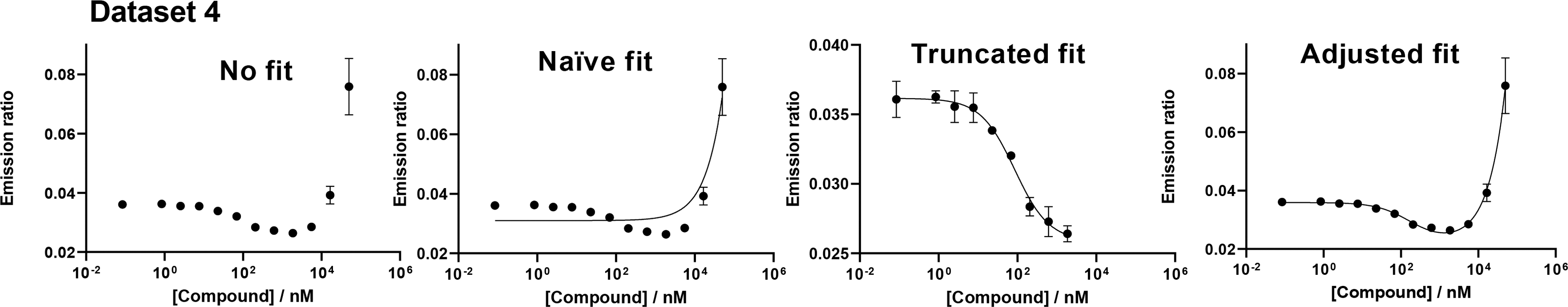
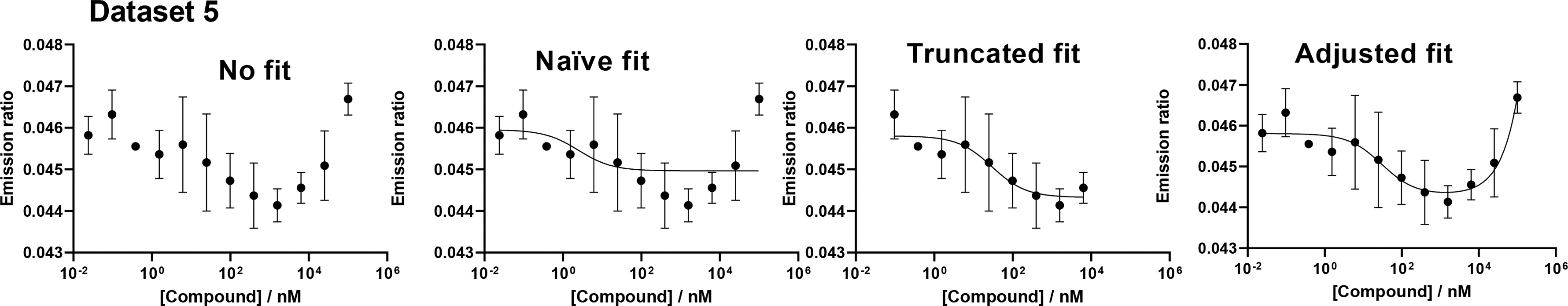
The three different fitting approaches to data sets 4 and 5 lead to largely different results. The naive fit should be avoided as it fails to generate any useful results, even if the R ² value appears to be reasonable in the case of data set 4 (which stresses that looking at the R ² alone is not enough to determine whether a fitting approach is suitable!). Data set 5 shows very noisy data, where the emission ratio range is quite small due to problems with the experimental setup. In this case it is not so clear which data points should be truncated and the IC₅₀ value changes depending on which data are omitted, making this approach problematic. On the contrary, with the adjusted fit, truncating data are not necessary, although the data should be reacquired to improve the confidence in the results. Note that the range of the emission ratio for data set 4, truncated fit, has been “zoomed in” compared with the two other approaches, to improve clarity. The best fit values are shown in bold and their corresponding 95% CI in bracket. Here NA stands for not applicable and describes the situation where it was not possible to calculate a 95% CI.

NA, not applicable.

Truncation of the Data Can Lead to Systematic Underestimation of IC₅₀ Values

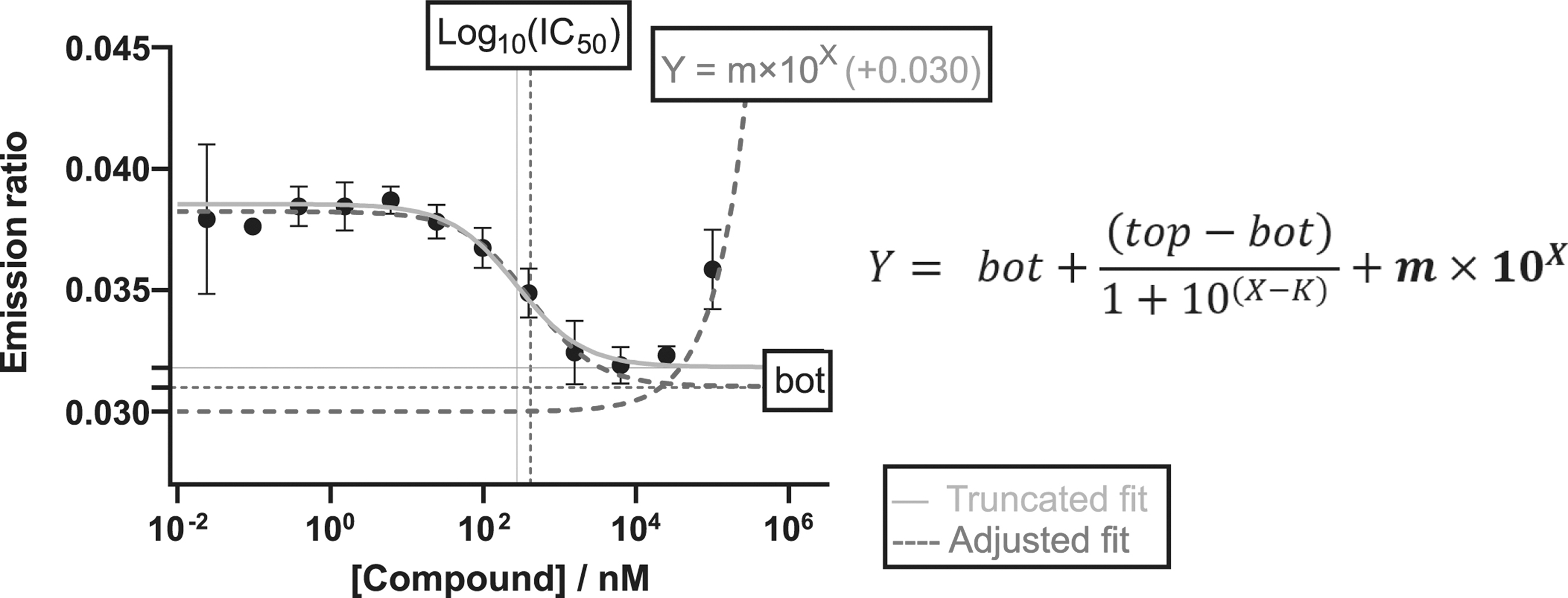
It was noticed that the IC₅₀ value is always smaller for the truncated fit compared with the adjusted fit approach. In Eq. (1), the values for the parameter bot should coincide with the plateauing of emission ratio values at high compound concentration. However, for the adjusted fit, the fluorescence values measured are the sum of the autofluorescence of the compound ( $Y = m \times 1 0^{X}$ ) and the FRET signal between the Eu-tagged antibody and the tracer ( $Y = b o t + \frac{(t o p - b o t)}{1 + {10^{(X - K)}}^{}}$ , Fig. 2). At low compound concentration, the contribution from $Y = m \times 1 0^{X}$ is very small, but as the compound concentration increases so does the autofluorescence of the compounds. As a result, the effective bot parameter should be smaller than when ignoring the autofluorescence of the compounds. Smaller bot parameters lead to larger IC₅₀ values compared with the naive or truncated fit (Fig. 2).

Fig. 2.

Accounting for autofluorescence of compounds in fluorescent-based kinase binding assays. On the left side, fluorescence intensity (emission ratio) from LanthaScreen™ kinase binding assay is plotted against compound concentration (logarithmic scale) and fitted with two different approaches. First, a truncated fit (solide grey), where the two last points at highest compound concentrations have been omitted for the fitting, as they do not follow the sigmoidal curve. In the second approach, the fitting method is adjusted by adding the term m × 10^X to the typical logistic function, to account for the fluorescence of the compounds (equation on the right). The adjusted approach does not require trimming the data and results in having slightly lower values for the parameter bot, resulting in slightly larger IC₅₀ values. Y is the fluorescent signal, and top and bot are parameters representing the minimum and maximum signal. X is the logarithmic concentration of the compound and K is the Log₁₀(IC₅₀) value of the reaction.

Based on the adjusted fit model, it appears that truncating data deviating from the fit with Eq. (1) leads to underestimation of the IC₅₀ value.

CONCLUSION

In the context of data fitting in a dose–response experiment, this article describes a simple yet effective adjustment of the typical fit with Eq. (1), to include the contribution from the autofluorescence of compounds. Of importance, this equation assumes a linear increase of the fluorescence with the compound concentration, which is well suited to water-soluble compounds, but has not been tested to describe the fluorescence drift linked to protein-compound aggregation or J-aggregation, sometimes affecting fluorescence-based assays.⁹ When a good signal is measured and compounds tested are not fluorescent, the classical naive approach is perfectly fine (e.g., data set 1) and should be preferred because of its simplicity. However, when working with fluorescent compounds, the naive approach does not describe the data adequately anymore and it becomes necessary to adapt the fitting method.

Traditionally, outliers were removed until fitting improved, and while this approach can be legitimate in some situation (e.g., data set 4) it can also lead to reproducibility issues. It was also shown that truncating data can lead to underestimation of the IC₅₀ values (Fig. 2) by neglecting the contribution of the compound fluorescence to the parameter bot at higher compound concentrations. For this reason, I believe that the adjusted fit Eq. (2) should be preferred over omitting data.

Natural science is facing a “reproducibility crisis” and among the many potential reasons specified, one finds selective reporting, poor analysis, and unavailability of raw data.¹⁰ I hope that Eq. (2) can simplify some of the analyses with fluorescent compounds. This adjusted approach is not a substitution for inspecting the data carefully, especially in situations where they behave in an unexpected manner. In the end, it will be up to the experimenters to find the balance between simplicity and correctness, to determine whether their data are good enough to be fitted with the naive approach, or if Eq. (2) is better suited instead.

To conclude, I would like to share the idea from George Box that: “All models are wrong, but some are useful.”¹¹

Footnotes

ACKNOWLEDGMENTS

I would like to thank my colleagues Jeanette Andersen and Espen Hansen at Marbio, for providing helpful comments on the manuscript.

AUTHORs' CONTRIBUTIONS

G.A.P. is responsible for all the work acquired and presented in this article: conceptualization, data acquisition, data curation, formal data analysis, writing and editing of the original article, and preparation of figures and tables.

DISCLOSURE STATEMENT

No competing financial interests exist.

FUNDING INFORMATION

This work was not supported by any grants or funding agencies.

SUPPLEMENTARY MATERIAL

Supplementary Data S1

Abbreviations Used

References

Cicenas

, Zalyte

, Bairoch

, et al. Kinases and cancer. Cancers, 2018; 10(3):63; doi: 10.3390/cancers10030063

Attwood

, Fabbro

, Sokolov

, et al. Trends in kinase drug discovery: Targets, indications and inhibitor design. Nat Rev Drug Discov, 2021; 20(11):839–861; doi: 10.1038/s41573-021-00252-y

Glickman

FJ.

Assay development for Protein Kinase Enzymes. In: Assay Guidance Manual [Internet]. (Markossian S, Grossman A, Brimacombe K, et al.) Eli Lilly & Company and the National Center for Advancing Translational Sciences: Bethesda, MD, USA; 2012. Available from: https://www.ncbi.nlm.nih.gov/books/NBK91991/ [Last accessed: April 2023].

Mason

, Spais

, Husten

, et al. Comparison of LanthaScreen Eu kinase binding assay and surface Plasmon resonance method in elucidating the binding kinetics of focal adhesion kinase inhibitors. Assay Drug Dev Technol, 2012; 10(5):468–475; doi: 10.1089/adt.2012.453

Lebakken

, Riddle

, Singh

, et al. Development and applications of a broad-coverage, TR-FRET-based kinase binding assay platform. J Biomol Screen, 2009; 14(8):924–935; doi: 10.1177/1087057109339207

Hill

. The possible effects of the aggregation of the molecules of hæmoglobin on its dissociation curves. J Physiol, 1910; 40(Suppl.):iv–vii; doi: 10.1113/jphysiol.1910.sp001386

Neubig

, Spedding

, Kenakin

, et al. International Union of Pharmacology Committee on Receptor Nomenclature and Drug Classification. XXXVIII. Update on terms and symbols in quantitative pharmacology. Pharmacol Rev, 2003; 55(4):597–606; doi: 10.1124/pr.55.4.4

Gaigalas

, Li

, Henderson

, et al. The development of fluorescence intensity standards. J Res Natl Inst Stand Technol, 2001; 106(2):381–389; doi: 10.6028/jres.106.015

Heo

, Murale

, Yoon

, et al. Recent trends in molecular aggregates: An exploration of biomedicine. Aggregate, 2022; 3(2):e159; doi: 10.1002/agt2.159

10.

Baker

. 1,500 scientists lift the lid on reproducibility. Nature, 2016; 533(7604):452–454; doi: 10.1038/533452a

11.

Box

GEP

. Science and statistics. J Am Stat Assoc, 1976; 71(356):791–799; doi: 10.1080/01621459.1976.10480949