Response of Atmospheric Biomarkers to NO x -Induced Photochemistry Generated by Stellar Cosmic Rays for Earth-like Planets in the Habitable Zone of M Dwarf Stars

Abstract

Understanding whether M dwarf stars may host habitable planets with Earth-like atmospheres and biospheres is a major goal in exoplanet research. If such planets exist, the question remains as to whether they could be identified via spectral signatures of biomarkers. Such planets may be exposed to extreme intensities of cosmic rays that could perturb their atmospheric photochemistry. Here, we consider stellar activity of M dwarfs ranging from quiet up to strong flaring conditions and investigate one particular effect upon biomarkers, namely, the ability of secondary electrons caused by stellar cosmic rays to break up atmospheric molecular nitrogen (N₂), which leads to production of nitrogen oxides (NO_x) in the planetary atmosphere, hence affecting biomarkers such as ozone (O₃). We apply a stationary model, that is, without a time dependence; hence we are calculating the limiting case where the atmospheric chemistry response time of the biomarkers is assumed to be slow and remains constant compared with rapid forcing by the impinging stellar flares. This point should be further explored in future work with time-dependent models. We estimate the NO_x production using an air shower approach and evaluate the implications using a climate-chemical model of the planetary atmosphere. O₃ formation proceeds via the reaction O+O₂+M→O₃+M. At high NO_x abundances, the O atoms arise mainly from NO₂ photolysis, whereas on Earth this occurs via the photolysis of molecular oxygen (O₂). For the flaring case, O₃ is mainly destroyed via direct titration, NO+O₃→NO₂+O₂, and not via the familiar catalytic cycle photochemistry, which occurs on Earth. For scenarios with low O₃, Rayleigh scattering by the main atmospheric gases (O₂, N₂, and CO₂) became more important for shielding the planetary surface from UV radiation. A major result of this work is that the biomarker O₃ survived all the stellar-activity scenarios considered except for the strong case, whereas the biomarker nitrous oxide (N₂O) could survive in the planetary atmosphere under all conditions of stellar activity considered here, which clearly has important implications for missions that aim to detect spectroscopic biomarkers. Key Words: M dwarf—Atmosphere—Earth-like—Biomarkers—Stellar cosmic rays. Astrobiology 12, 1109–1122.

1. Introduction

M dwarf stars are numerous, long-lived, and have relatively high planet-to-star luminosity ratios. Therefore, they have been suggested as promising targets for searches for habitable planets (e.g., Scalo et al., 2007; Rauer et al., 2011). Such systems will, however, possess a close-in habitable zone (HZ) where, for example, coronal mass ejections, which are frequent for active M dwarf stars, may erode the planetary atmosphere (Khodachenko et al., 2007; Lammer et al., 2007, 2008). For a young planet, the dense and fast stellar wind can play a similar role (Grießmeier et al., 2010). Clearly, for life to develop, habitable conditions must be maintained for sufficiently long timescales. More modeling studies of, for example, atmospheric escape and the long chemical development of the atmosphere are required to gain more understanding. Here, we concentrate on the effect of high stellar cosmic rays (SCRs) on biomarker molecules of terrestrial exoplanets.

The particle flux of galactic cosmic rays (GCRs) to Earth-like planets in the HZ around M dwarf stars was studied by Grießmeier et al. (2005, 2009), and resulting effects on atmospheric chemistry were discussed by Grenfell et al. (2007a) and Grießmeier et al. (2009, 2010). In the present work, we extend these studies and look at the effect of SCRs caused by stellar activity ranging from quiet up to strong flaring conditions on the atmospheric chemistry. A motivation for this work is that SCRs could be especially dominant compared with GCRs for young, active M dwarf stars. In these cases, not only are SCRs especially significant, but furthermore the strong stellar magnetic fields lead to strong attenuation of the GCRs. We focus on the particle effects under differing conditions. In a recent work, Segura et al. (2010) investigated the photochemistry induced on such Earth-like atmospheres by modeling the high-energy radiation and charged-particle effects associated with a single, strong flare. They showed that stellar UV radiation emitted during the flare does not significantly affect the ozone column depth of the planet. We build on their work by assuming a harder criterion, namely, constant flaring conditions (see below) for our considered planetary atmosphere. Also, whereas the Segura work estimated NO_x production from observed X-ray proxies, in our work we applied a theoretical air-shower approach to determine such NO_x production directly (as we will show, both approaches compare quite well). Finally, compared with the Segura et al. work, we build on and extend the chemical analysis, providing new insight into the responses of biomarkers, related species, and UV protection of the planetary surface. Section 2 describes the models, Section 3 presents results, and Section 4 draws conclusions with regard to the response of atmospheric biomarkers and their spectral signatures.

1.1. Cosmic rays (CRs) and magnetic fields

Galactic cosmic rays travel from their source regions (e.g., supernovae) through the interstellar medium and penetrate the stellar magnetic field (for a good review, see Scherer et al., 2002). Heavier CR particles consisting of, for example, helium, carbon, and iron nuclei (Seo et al., 1991; Ziegler, 1996; Gloeckler et al., 2009) are known, but their fluxes are lower by at least an order of magnitude compared with the proton fluxes. High-energy SCRs can be richer in heavier elements (Smart and Shea, 2002). Our work however, assumes the CR particles are protons.

Penetration of CRs through a planet's protective magnetosphere and associated effects are the subject of a rich body of literature. Melott and Thomas (2011) and Dartnell (2011) and references therein provided reviews. Both heliosphere and magnetosphere fields are variable in time and space. In an exoplanetary context, a planet with an Earth-like magnetic field will likely direct CRs with modest energies (up to several hundreds of megaelectronvolts) to its polar regions, as is the case for the auroral zones of Earth (see Tarduno et al., 2010, for a review), whereas for planets with weak or no magnetic fields, high-energy CRs could also impinge at lower latitudes.

1.2. Interactions of CRs with atmospheres and biomarkers

Cosmic rays interact with planetary atmospheres in a range of ways. They can induce ionization as observed, for example, on Titan and Venus (Dartnell, 2011) and in association with lightning (e.g., Dwyer, 2005), acid rain, and cloud formation on Earth (e.g., Svensmark and Christensen, 1997). A 3-D model would be required for a full description, although a 1-D study is an adequate first step, since the necessary boundary conditions for a 3-D study are completely lacking for extrasolar planets. On Earth, O₃ features a seasonal cycle where winter/spring column values (Brasseur et al., 1999) are enhanced by about 50% due to weak photolytic loss in winter. It has a latitudinal gradient being produced in Earth's tropics and transported by the meridional circulation to the pole where its column value peaks. At cold polar latitudes in winter, O₃ is rapidly lost via fast catalytic chlorine cycles (e.g., WMO, 1994). Ozone varies in altitude—in Earth's troposphere it is produced by the smog mechanism (Haagen-Smit, 1952). In Earth's stratosphere, O₃ is produced by the Chapman mechanism (Chapman, 1930). In the mesosphere and thermosphere, where O₃ is affected by fast hydrogen-oxide loss cycles and direct photolytic loss, it displays a diurnal cycle. A discussion and implications for future 3-D model studies is presented in the Discussion.

Solar proton events (SPEs) can form NO_x (from N₂) and HO_x (from O₂), which affect O₃ via chemical reactions. NO_x (in the form of NO) formation on Earth from SPEs occurs typically at 70–100 km—here it can be quickly photolyzed, but in winter it survives in the dark polar vortex to be transported slowly (over periods of typically several weeks) down to the mid stratosphere where the O₃ layer resides. In spring, the vortex breaks up, and the enhanced NO_x is transported to lower latitudes, where it encounters sunlight, which initiates catalytic O₃ loss cycles. The removal timescales of NO_x and HO_x are typically a couple of weeks in Earth's mid stratosphere. In Earth's troposphere, at very high NO_x abundances of about a few parts per million, O₃ is removed directly. At more modest NO_x abundances of about 1000 times lower, smog O₃ is produced.

Solar proton events on Earth have been documented to perturb stratospheric NO_x at high latitudes and, hence, may have a significant impact upon O₃. For example, the large 1989 SPE led to a 1–2% decrease in the O₃ column averaged over 50° to 90°N (Jackman et al., 2000), whereas the significant 2003 SPE led to a lowering in local O₃ by several tens of percent in the mid to upper stratosphere (Jackman et al., 2005). In recent years, numerous 3-D photochemical modeling studies of SPEs have been applied to Earth's atmosphere, for example, Jackman et al. (2011) and references therein simulated charged particle precipitation during the January 2005 ground level event, calculating NO_x abundances of greater than 50 parts per billion by volume in the polar mesosphere. Satellite observations were also simultaneously employed to study the perturbed atmospheric composition and the relaxation of active oxides into key reservoir molecules such as HNO₃ and H₂O₂.

2. Description of Model Approach, Model, and Runs

Model approach

First, we calculate the top-of-atmosphere (TOA) global mean SCR fluxes based on observations of solar particles taken above Earth's magnetosphere for an unmagnetized planet located in the habitable zone around an M dwarf star (MHZ). Second, these SCR fluxes induce an enhanced NO_x production in the planetary atmosphere as described by the air-shower approach in the radiative convective photochemical column model (Section 2.1). Finally, the resulting chemical concentration and temperature profiles from the column model are input into a line-by-line spectral model to calculate theoretical emission spectra (Section 2.2).

2.1. Coupled climate-chemistry atmospheric column model

We use the new model version of the coupled chemistry-climate 1-D atmospheric model of Rauer et al. (2011) and references therein. Recent model updates since the work of Grenfell et al. (2007a, 2007b) include a new offline binning routine for calculating the input stellar spectra and a variable vertical atmospheric height in the model (more details are given in Rauer et al. (2011). There are two main modules, namely, a radiative-convective climate module and a chemistry module.

The climate module is a global-mean stationary, hydrostatic column model of the atmosphere

The model pressure grid ranges from the surface up to 6.6×10⁻⁵ bar (for Earth this corresponds to a height of about 70 km). Initial composition, pressure, and temperature profiles are based on modern Earth. The radiative transfer calculation is based on the Rapid Radiative Transfer Module (RRTM) for the thermal radiation. This scheme applies 16 spectral bands by using the correlated k-method for the major atmospheric absorbers. The RRTM validity range (see Mlawer et al., 1997) for a particular altitude corresponds to Earth's modern climatological mean temperature±30 K for pressures from 10⁻⁵ to 1.05 bar and for a CO₂ abundance from modern-day up to×100 that value. The shortwave radiation scheme consists of 38 spectral intervals for the major absorbers and includes Rayleigh scattering for N₂, O₂, and CO₂ with cross sections based on Vardavas and Carver (1984). A constant, geometrical-mean, solar-zenith angle=60° is used. In the troposphere, a moist adiabatic lapse rate is assumed where the radiative temperature gradient is larger than the moist adiabatic gradient. Humidity in the troposphere is based on Earth observations (Manabe and Wetherald, 1967). For the Earth-around-the-Sun scenario, a solar spectrum based on Gueymard (2004) is employed. For the M dwarf scenarios, an AD Leo stellar spectrum is derived from observations by Pettersen and Hawley (1989) as taken from the IUE satellite and observation by Leggett et al. (1996) in the near IR and based on a nextGen stellar model spectrum for wavelengths beyond 2.4 microns (Hauschildt et al., 1999). The climate effects of clouds are not included explicitly, although these are considered in a straightforward way by adjusting the surface albedo to a value of 0.21 in all runs, that is, for which the mean surface temperature of Earth (288 K) was attained for the Earth control run. Starting values (T, p) for the climate module were based on the U.S. Standard Atmosphere (COESA, 1976). The climate module ran to convergence; then outputs temperature, pressure, and water abundances were taken as input for the chemistry module.

The chemistry module was described by Pavlov and Kasting et al. (2002)

The current scheme includes 55 chemical species for 212 reactions with chemical kinetic data taken from the Jet Propulsion Laboratory report (Sander et al., 2003). The kinetic data are typically measured from about 250 to 400 K, although each reaction has its own stated range. Three-body reactions are usually measured in an N₂-O₂ bath gas (e.g., Sander et al., 2003). Note that different rate constants by up to about a factor of 10 may be expected for reactions in, for example, CO₂-dominated atmospheres, although we do not consider these here. The chemistry module assumes a planet with an Earth-like development, that is, with an N₂-O₂ dominated atmosphere, and so on. The reaction scheme is designed to reproduce modern Earth's atmospheric composition with a focus on biomarkers (e.g., O₃, N₂O) and major greenhouse gases such as CH₄. It therefore includes fast nitrogen-oxide and hydrogen-oxide reactions and their reservoir species, reproducing Earth's atmospheric O₃ abundance, as well as the major sources and sinks of hydroxyl (OH), reproducing the atmospheric CH₄ profile. The chemical module calculates the steady-state solution of the usual 1-D continuity equations by an implicit Euler method. Atmospheric mixing between adjacent gridboxes is parameterized via Eddy diffusion coefficients (K). K is set to 10⁵ cm² s⁻¹ from the surface up to z=10 km, decreasing to K=10^3.5 cm² s⁻¹ at z ∼ 16 km then increasing up to K=10^5.5 cm² s⁻¹ at z ∼ 64 km. From a total of 55 chemical species, 34 are “long-lived,” that is, their concentrations are obtained by solving the full continuity equation. A further 16 species are “short-lived,” that is, their concentrations are calculated exclusively from the long-lived species concentrations by assuming chemical steady state, that is, equating production rates with loss rates for each short-lived species. Finally, the remaining, so-called “isoprofile species” are set to constant abundances in all gridboxes, namely, CO₂=3.55×10⁻⁴, O₂=0.21, and N₂ ∼ 0.78 volume mixing ratio (vmr).

Boundary conditions in the chemistry module were based on reproduction of the modern Earth atmospheric composition and included constant surface biogenic (CH₃Cl, N₂O) and source gas (CH₄, CO) species (see Grenfell et al., 2011, for more details). Also included are modern-day tropospheric lightning emissions of nitrogen monoxide (NO), volcanic sulfur emissions of SO₂ and H₂S, and a constant effusion flux of CO and O at the upper model boundary, which represents the photolysis products of CO₂. Surface removal of long-lived species via dry and wet deposition is included via deposition velocities (for dry deposition) and Henry's law constants (for wet deposition). The chemistry module ran to convergence and then output its greenhouse gas abundances to the climate module. This whole process, that is, exchange of data between the two modules, is repeated until the chemical concentrations and the atmospheric temperature and pressure structure converge.

The cosmic ray scheme

Starting with the incoming TOA time-average proton fluxes calculated by the Cosmic Ray Proton Flux (CRPF) model (Grießbmeier et al., 2005) (Fig. 1), we calculated NO (hence NO_x) production in our atmospheric column model as in Grenfell et al. (2007a). We consider thereby only incoming proton energies of 64 MeV and above. Somewhat lower energies down to ∼10 MeV may also affect Earth's atmosphere but mostly at altitudes above the mesosphere, not considered in our work. The CRPF model was originally designed to simulate the detailed passage of a large number of high-energy proton trajectories through Earth's magnetosphere. In its current implementation, the scheme is not suitable for calculating the above-mentioned lower energies. Adding these would increase NO_x generation and O₃ loss, so our results can be regarded as conservative in this sense.

FIG. 1.

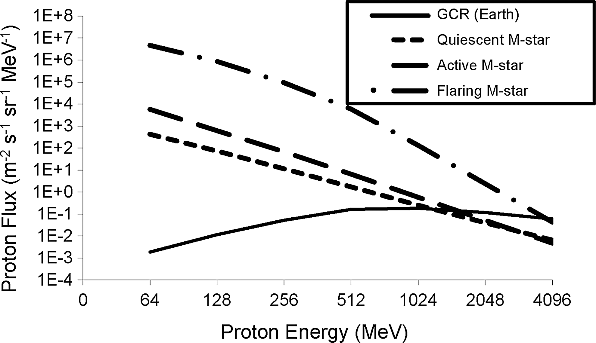
Cosmic ray proton spectra normalized to 0.153 AU and the average GCR spectra for Earth at 1 AU (solid line).

The impinging protons produce secondary electrons (e⁻), hence, NO_x, via \documentclass{aastex}\usepackage{amsbsy}\usepackage{amsfonts}\usepackage{amssymb}\usepackage{bm}\usepackage{mathrsfs}\usepackage{pifont}\usepackage{stmaryrd}\usepackage{textcomp}\usepackage{portland, xspace}\usepackage{amsmath, amsxtra}\pagestyle{empty}\DeclareMathSizes{10}{9}{7}{6}\begin{document} \begin{align*} { \rm N}_2 + { \rm e}^ - \rightarrow 2{ \rm N} + { \rm e}^ - \\ \ \, { \rm N} + { \rm O}_2 \rightarrow { \rm NO} + { \rm O}\end{align*} \end{document}

The resulting NO fluxes were then calculated interactively in the atmospheric column model. An important parameter (k) is defined as the number of atomic nitrogen atoms produced on average when one nitrogen molecule is destroyed. Values of k have been suggested in the range k=0.96 (e.g., Nicolet, 1975) up to k=1.25 (e.g., Porter et al., 1976; Jackman et al., 1980). We assumed one NO_x produced per N₂ destroyed at all heights (i.e., k=1). We further assumed a third-power law for the secondary electron energy spectrum (Bichsel et al., 2005) with a proton penetration profile based on Gaisser and Hillas (1977) (their Fig. 2). For proton energies at and above 256 MeV, we assumed a proton attenuation length (PAL) of 80 g cm⁻², and we further assumed a PAL_max=150 g cm⁻² (defined as the column mass obtained by integrating from the TOA down to the altitude where the shower has its maximum). For the three lower proton energy levels of 256, 128, and 64 MeV, which are important for stellar particles (see Fig. 1), we assumed PAL=10⁻³, 1, 2 g cm⁻², PAL_max=10⁻², 5, 25 g cm⁻², respectively (Amsler et al., 2008). We assumed an electron attenuation length of 40 g/cm² for all energy levels, also based on Amsler et al. (2008). The bulk of measured PAL data for Earth's atmosphere is obtained at energies at least several orders of magnitude higher. In our study, values were therefore obtained by extrapolation. The Particle Data Group (2002) report suggested that the PAL and PAL_max values quoted for the three lowest energy levels in our work are uncertain by around a factor of 10. Therefore, NO_x-catalyzed O₃ loss calculated in our work may be an underestimate. This caveat therefore is not likely to change the conclusions for the flaring run, where all O₃ is destroyed. We performed a parameter variation where PAL values were decreased by up to two orders of magnitude. As a result, the maximum of our CR-induced NO_x production moved from about 15 km height up to about 22 km (not shown).

FIG. 2.

Number of secondary electrons (S _e) produced relative to the shower maximum (Nel_max), where Nel_max=3 for all energies. Data are shown for run 1, which is the case for Earth orbiting the Sun including the effect of GCRs (“Earth GCR run”).

It is not possible to validate a stationary model in terms of, for example, O₃ depletion by using SPE measurements for Earth since these results are time-dependent. However, we present here a comparison of ion-pair production. Jackman et al. (2005) (their Fig. 1) reported peak ion-pair production for Earth of about 10⁴ ions cm⁻³ s⁻¹ at 60–70 km dropping to about 10² ions cm⁻³ s⁻¹ at ∼30 km based on GOES-11 observations of the October 2003 SPE. By comparison, our column model (SPE Earth conditions) calculated (2–4)×10² ions cm⁻³ s⁻¹ above 60 km, ∼5×10⁴ at 30 km, and a peak production of ∼7×10⁴ ions cm⁻³ s⁻¹ in the lower stratosphere. In summary, our stationary model overestimates peak ion production for Earth's mid atmosphere since we simulate constant flaring conditions, although this shortcoming is expected to be less important for the M star constant flaring case. In a different approach, Segura et al. (2010) aimed to model a transient single flare from AD Leo—the resulting NO_x production rates are, however, rather similar to our values (as discussed later in the text).

2.2. Theoretical line-by-line spectral model

The SQuIRRL (Schwarzschild Quadrature InfraRed Radiation Line-by-line) code (Schreier and Schimpf, 2001) was originally designed for high-resolution radiative transfer modeling in the IR assuming a spherical atmosphere (for an arbitrary observation geometry, instrumental field-of-view, and spectral response function). Assuming local thermodynamic equilibrium, a Planck function (with appropriately level temperatures) is used as the emission source. The simulated atmosphere is assumed to be cloud and haze free without scattering. SQuIRRL has been verified via extensive intercomparisons with other radiative transfer codes (e.g., von Clarmann et al., 2002; Melsheimer et al., 2005). By using molecular spectroscopic line parameters from the HITRAN 2004 (Rothman et al., 2005) database, absorption coefficients are computed with continuum corrections. The emission spectra are calculated assuming a pencil beam at a viewing angle of 38 degrees as adopted, for example, by Segura et al. (2003).

2.3. Application of a stationary SCR model to active M dwarf star conditions

A stationary atmospheric column model approach assumes that the biomarker chemical responses are slow compared with the stellar variability. Therefore, we now discuss and compare biomarker photochemical timescales with stellar variability timescales for AD Leo. Note, in our model study we consider only NO_x production from CRs (and not the effect of the change in UV during flaring conditions) and its influence upon the biomarkers. Nevertheless, we briefly discuss stellar (UV) variability of M dwarf stars in order to investigate the applicability of our time-independent model.

We perform a timescale analysis where we make the assumption that the relevant removal timescale for perturbed NO_x (induced by CRs) occurs via oxidation into nitric acid via the reaction NO₂+OH+M→HNO₃+M, where M, the total atmospheric number density, denotes a third body as a collision partner to remove excess vibrational energy. We also assume that the initial NO_x forcing (enhancement via CRs) occurs only once and is immediately followed by removal via the oxidation reaction—this is also a reasonable assumption for a strong SPE in Earth's stratosphere. We note, however, that for M dwarf scenarios the above assumptions should be further explored by time-dependent models. For example, the UV environment of the planet's atmosphere will influence how NO_x is removed, for example, for changed UVB environments; other NO_x reservoirs (and not HNO₃ as on Earth) could play a greater role in NO_x removal. Regarding NO_x formation via CRs, the forcing timescale will depend also on, for example, the magnitude and frequency of the stellar flares. For example, for an Earth-like planet orbiting in the HZ around AD Leo, typical flares there would be considered large (in terms of total flare energy) compared to those observed on Earth and may occur 3–4 times per Earth day (see the following discussion). However, there also exist higher energy flare events that occur every ∼(1–2) Earth weeks (e.g., Güdel et al., 2003, their Fig. 3). Although with the above caveats in mind, the following timescale analysis, however, assumes as a first estimate an Earth-like NO_x relaxation into HNO₃ with a single NO_x-forcing event, as described in the following section.

Biomarker photochemical timescales

We focus in the mid stratosphere at z=30 km since this is where the O₃ layer peaks. Defining the NO_x removal timescale, τ_NO2 (30 km)=[NO₂]/k[OH][NO₂] gives column model values of ∼12 days (∼43 days) for our Earth-orbiting-the-Sun scenario (Earth-like planet orbiting AD Leo, flaring scenario). The factor 3.6 increase here reflects the lowering in [OH] for M dwarf star scenarios, due to the weaker UVB output of the central star, as already discussed, for example, by Segura et al. (2005). The above timescales are probably, however, underestimates, since the resulting HNO₃ can photolyze to release its NO_x back into the atmosphere. Then the effective timescale for NO_x removal can be much longer—up to a few years. For example, Thomas et al. (2005a, 2005b) and Ejzak et al. (2007) showed that atmospheric O₃ depletion from enhanced NO_x (from simulated, close-by gamma-ray bursts) lasts for a long time. O₃ depletion is constant for ∼2 years, and even after 5–7 years, 10% depletion remains. The Ejzak et al. study further suggests that strong ionizing events led to a ∼(33–37)% maximum decrease in the O₃ column. In summary, we estimate biomarker timescales of (Earth) months to years in the mid stratosphere, decreasing in the upper stratosphere to mesosphere down to several Earth weeks.

AD Leo variability timescales

Khodachenko et al. (2007) suggested that AD Leo emits more than 36 coronal mass ejections per day. Regarding the stellar photon flux variability, the total energy of the flare in our flaring scenario corresponds to 1.2×10³² erg (see e.g., Gopalswamy, 2006), assuming quadratic scaling of CRs with the planet at 0.153 AU. For such flares, this energy corresponds to a flare frequency for AD Leo (see Audard et al., 2000) of several per day, consistent with Houdebine et al. (1990). However, the Audard study (their Fig. 1) also indicated isolated, very large flaring events occurring on timescales of up to 1–2 Earth weeks, as already mentioned (for more details see also Güdel et al., 2003). For such large flaring events, the stationarity assumption of our model, especially in the upper layers, could be weak. A preliminary analysis of our model results for the AD Leo “flaring run,” however, suggested that removal of NO_x into HNO₃ is still an important chemical process in the stratosphere and that the removal is slower than on Earth. However, it is interesting to revisit this issue with a time-dependent model and to calculate the resulting timescales for the removal of NO_x into its photochemical reservoir molecules.

Diurnal O₃ observations on Earth

It is well known that O₃ diurnal variations are low in Earth's middle atmosphere. This suggests that the O₃ response to changes in UV on timescales of ∼12 h are negligible, which supports the case for applying a stationary model at least for these particular conditions. Clearly, this depends on the planetary rotation rate and is no longer valid for faster rotating planets. We expect the rotation rate of planets considered in this work to be comparable to, or lower than, that of Earth, as discussed.

2.4. About the runs

In this study, we assumed that our hypothetical Earth-like planet is positioned in the MHZ at 0.153 AU, the distance where integrated radiative energy fluxes of our adopted input stellar (AD Leo) spectrum are equal to the solar constant.

Run 1: Earth orbiting the Sun at 1 AU distance (solar spectrum) conditions, that is, with biomass emissions reproducing modern Earth's biosphere and with TOA galactic cosmic ray (GCR) fluxes as calculated by the CRPF model (see Section 2.1 and Grießmeier et al., 2005, for more details) for the magnetized planet Earth ( Earth GCR run ).

Run 2: Same as run 1 but with M dwarf stellar spectrum (AD Leo) ( GCR M dwarf star run ).

Run 3: Same as run 2 but with GCR input replaced with interplanetary SCRs for an unmagnetized planet based on Kuznetsov et al. (2005) scaled to 0.153 AU by using particle observations over approximately 1 year of the Sun during the minimum of the 11-year solar cycle ( Quiescent M dwarf star SCR run ).

Run 4: Same as run 3 but using particle observations of the Sun during the maximum of the 11-year solar cycle ( Active M dwarf star SCR run ).

Run 5: Same as run 4 but with SCRs based on Smart and Shea (2002) scaled to 0.153 AU by using peak particle observations of the Sun during a SPE ( Flaring M dwarf star SCR run ).

Run 6: As for run 5 but with a reduced Eddy mixing coefficient by a factor of 10.

Run 7: As for run 5 but neglecting Rayleigh scattering.

Cosmic ray input data for the runs

For the quiet and active star scenarios, we employed the spectra of Kuznetsov et al. (2005) at 1 AU (their Fig. 2). For the flaring M dwarf star case, we used data measured at 1 AU by the spacecrafts GOES 6 and 7 on September 30, 1989 (Smart and Shea, 2002, their Fig. 11). Particle fluxes are determined by a small number of events with very high values, which makes averaging challenging. The number of events varies with the solar cycle, with higher fluences for about 7 years, followed by a quieter period of about 4 years (Feynman et al., 1993, their Figs. 1 and 2). However, the fluence during the latter period is not negligible, so that the division into two such categories is debated (Kuznetsov et al., 2001). These spectra do not correspond to a continuous particle stream from the Sun but to average over all small, medium, and large events that may happen during 1 year.

The variation of the SCR flux as a function of distance from the source is not known for stars other than the Sun. For this reason, we base the distance dependence of the particle flux on that observed for the Sun. Solar particle fluxes have a strong maximum near the region where they are generated. As they travel outward, this feature is diluted. This results in a longer event duration at large orbital distances and reduces the instantaneous flux during the event due to particle conservation. The effect is stronger for lower-energy particles, as seen in observations (Hamilton, 1977, their Fig. 10) and in numerical simulations (Hamilton et al., 1990, their Fig. 1; Lario et al., 2000, their Fig. 9). Feynman and Gabriel (1988) established a first set of power laws at distance d<1 AU for the peak flux, f _peak, and for the event fluence, fl _event (i.e., the number of particles integrated over the whole time of the event): \documentclass{aastex}\usepackage{amsbsy}\usepackage{amsfonts}\usepackage{amssymb}\usepackage{bm}\usepackage{mathrsfs}\usepackage{pifont}\usepackage{stmaryrd}\usepackage{textcomp}\usepackage{portland, xspace}\usepackage{amsmath, amsxtra}\pagestyle{empty}\DeclareMathSizes{10}{9}{7}{6}\begin{document} \begin{align*} f_{ \rm peak} ( d ) = f_{ \rm peak} ( 1 \ { \rm AU} ) * ( d / 1 \ { \rm AU} ) ^{ \alpha} \\ fl_{ \rm event} ( d ) = f l_{ \rm event} ( 1 \ { \rm AU} ) * ( d / 1 \ { \rm AU} ) ^{ \beta}\end{align*} \end{document}

where α=(−3 to −2), β=(−3 to −2). In the range d=(0.65 to 4.92) AU, Hamilton et al. (1990) suggested that for particles with energies of 10–20 MeV, α=(−2.9 to −3.7) and β=(−1.8 to −2.4), which is in good agreement with their theoretical model. More recently, Lario et al. (2006) suggested for d<1 AU [based on 72 observations by Helios 1, Helios 2, and the Eighth Interplanetary Monitoring Platform (IMP-8)], that α=(−2.7 to −1.9) and β=(−2.1 to −1.0). They also stated that previous models did not take into account a focusing effect, which is important for d<1 AU. From numerical modeling, Ruzmaikin et al. (2005) concluded that α is energy-dependent, that is, α=− 2.6 at 10 MeV, which becomes more negative at higher energies, that is, α=−2.9 at 100 MeV (see their Fig. 4). Lario et al. (2006), on the other hand, suggested a more negative α at lower energies. Considering the uncertainties, we will use an energy-independent value. In our steady-state study, the more relevant quantity is the event fluence and not the peak flux because our model converges to a steady state. We therefore used the fluence equation above and adopted a mean value for β=−2.0.

3. Results

3.1. Top-of-atmosphere CR energy spectra and nitrogen monoxide (NO) production

Figure 1 shows the energy spectrum for primary particles impinging at the top of the planetary atmosphere calculated by the CRPF model. The Earth-orbiting-the-Sun-with-GCRs (run 1, hereafter “Earth GCR”) simulation shows enhanced fluxes at the higher energies, whereas the SCR fluxes in the other scenarios dominate the lower energy regime. Figure 2 shows the number of secondary electrons relative to the shower maximum as a function of incoming proton energy for run 1 (Earth GCR). Above 512 MeV, the energy curves overlap because input parameters (e.g., the maximum attenuation length, X _max) do not vary over this energy range. The high-energy (>512 MeV) CRs penetrate deepest into the atmosphere, leading to secondary electron shower production with values peaking at ∼0.5 in the upper troposphere at about 0.15 bar. With decreasing energy of the incoming protons, atmospheric penetration becomes weaker, and the peak value shifts to higher altitudes, that is, in the stratosphere and mesosphere.

Figure 3 shows the nitrogen monoxide (NO) atmospheric production rates from CRs (run 6 is similar to run 5 and thus not shown). For Earth, GCR simulation (run 1) peak NO production occurs near the tropopause (at ∼11 km). This is because the GCR energy spectrum (Fig. 1) has large values at high energies, which favor secondary electron production deep in the atmosphere (see Fig. 2). For the runs with quiescent and active conditions, peak NO production occurs in the mid stratosphere between 0.03 and 0.04 bar (∼20 to 22 km). This is because their energy spectrum (Fig. 1) is overall weaker than the Earth GCR case, producing secondary electrons at higher atmospheric levels (Fig. 2). The extreme “flaring” case in Fig. 3 features maximum NO production somewhat lower in the atmosphere at around 0.05 bar.

FIG. 3.

Nitrogen monoxide (NO) production rate varying throughout the atmosphere.

The rates shown in Fig. 3 lead to a concentration of NO for the flaring case in run 4 of 2×10¹⁴ molecules cm⁻³ (∼5×10⁻⁴ volume mixing ratio) in the mid stratosphere. This value corresponds to within about a factor of 2 to the peak concentrations calculated by Segura et al. (2010) in this region (see their Fig. 8, lower panel). The agreement is good given that we adopt independent methods, that is, Segura et al. use a proxy approach based on X-ray observations and simulate a single large flare, whereas we use a theoretical air shower method as previously described and assume constant, strong background flaring conditions (see also Grenfell et al., 2007a).

3.2. Column amounts of biomarkers and related compounds

Observations for Earth suggest that tropospheric NO increases lead to O₃ increases via the smog mechanism (Haagen-Smit, 1952), whereas stratospheric NO increases lead to catalytic loss of O₃ (Crutzen, 1970). NO_x and O₃ interact in different ways in the troposphere, depending upon atmospheric conditions (e.g., UV, NO_x, hydrocarbon abundances). A null cycle involving NO_x recycles O₃ as follows: \documentclass{aastex}\usepackage{amsbsy}\usepackage{amsfonts}\usepackage{amssymb}\usepackage{bm}\usepackage{mathrsfs}\usepackage{pifont}\usepackage{stmaryrd}\usepackage{textcomp}\usepackage{portland, xspace}\usepackage{amsmath, amsxtra}\pagestyle{empty}\DeclareMathSizes{10}{9}{7}{6}\begin{document} \begin{align*} { \rm NO} + { \rm O}_3 \rightarrow { \rm NO}_2 + { \rm O}_2 \\ { \rm NO}_2 + hv \rightarrow { \rm NO} + { \rm O} \\ { \rm O} + { \rm O}_2 + { \rm M} \rightarrow { \rm O}_3+ { \rm M} \\ \- - - - - - - - - - -\\ \qquad net: \ { \rm null}\end{align*} \end{document}

The null cycle recycling tropospheric O₃ competes with the established “smog cycle,” producing O₃ in which volatile organic compounds (VOCs) are oxidized by OH in the presence of NO_x and UV. There are three main regimes: firstly, where VOC abundances are at a premium for O₃ production (VOC-controlled); secondly, where NO_x is at a premium (NO_x-controlled); thirdly, in urban areas where NO_x abundances are very high (greater than about 10⁻⁶ vmr). In the latter regime, the removal reaction, NO₂+OH+M→HNO₃+M, lowers OH, which is a key player in the smog cycle and, hence, can effectively lower smog O₃ production, leading to a significant O₃ decrease.

Figure 4 shows column values of some important biomarkers and greenhouse gases. Ozone (O₃) columns are reduced by 39% for the quiescent M dwarf star case (run 3) compared with the Earth GCR case (run 1). The active M dwarf star case (run 4) features a 63% reduction compared with run 1. This suggests that the stronger CR-induced NO_x effect in run 4 can lead to more O₃ loss compared with run 2. The “flaring” M dwarf star extreme case (run 5) leads to almost complete removal of the O₃ atmospheric column, by more than 99% compared with the Earth GCR run, suggesting that the enhanced NO_x photochemistry in this run can act as a major sink for the O₃ biomarker.

FIG. 4.

Column values of biomarkers and greenhouse gases in Dobson Units (DU) (1 DU=2.69×10¹⁶ molecules cm⁻²).

The main chemical sink for O₃ switched from the familiar catalytic cycles (Earth GCR run 1) to the single (noncatalytic) titration reaction: NO+O₃→NO₂+O₂ for the “flaring” case (run 5). A similar effect is observed on Earth in large cities with very elevated NO abundances (see e.g., Shao et al., 2009). The main O₃ source in all runs proceeds via O+O₂+M→O₃+M, since this is the only reaction that forms O₃ in our model. However, the main source of atomic oxygen (O) for the above reaction changes from the familiar photolysis of O₂ in the Earth GCR case (run 1) to the photolysis of NO₂ via NO₂+hν→NO+O for the flaring case. Overall, ozone loss for the flaring case was strongly enhanced by CR chemistry.

Ozone can be produced or destroyed depending, for example, on the incoming TOA stellar radiative flux and the planetary atmospheric composition. In regions where UV is strong enough to photolyze efficiently, O₂ (e.g., in Earth's stratosphere) enhanced NO is expected to destroy O₃ via catalytic cycles. In regions where UV is less strong and hydrocarbons and NO_x are in excess of a few tens to hundreds of parts per trillion by volume, the smog mechanism will operate, and enhanced NO can lead to more O₃ production. Our results suggest that this effect could be sensitive to changes in the CR input spectrum. For example, Fig. 3 shows that the peak NO production rate shifts from the upper troposphere for the “flaring” run to the upper stratosphere for the quiescent run.

Methane (CH₄) columns for the M dwarf star cases show a large increase compared with the GCR Earth results. An important effect is a decrease in the hydroxyl (OH) radical abundance, an important atmospheric sink for CH₄. For example, the OH amount at the planetary surface is reduced by about 3 orders of magnitude in run 3 compared with the Earth GCR case (run 1). The OH reduction is related to a weakening in the well-known OH-forming reaction, H₂O+O¹D→2OH, for the M dwarf star cases compared with run 1 because the lower UVB output from the M dwarf star led to a lowering in atmospheric excited oxygen (O¹D) abundances1 and, hence, a slowing in this reaction, since O¹D is produced photolytically. In summary, the main effect is that less UVB leads to less OH and, therefore, more CH₄ for the M dwarf star cases. Segura et al. (2005) also discussed CH₄ perturbations associated with OH, and as was the case in our work, they also calculated large CH₄ abundances of ∼4×10⁻⁴ vmr at the planetary surface for their scenarios of Earth-like planets orbiting M dwarf stars. Our results suggest that the active case (run 4) and the flaring case (run 5) feature lower CH₄ columns than the quiescent case (run 3) (see also Section 3.3). Note that the biomarker chloromethane (CH₃Cl), like CH₄, is emitted at the surface and is removed from the atmosphere mainly via reaction with OH and via photolysis. CH₃Cl is, however, much more reactive than CH₄, being removed from the atmosphere about 8 times faster. Due to their similar photochemistry, CH₃Cl and CH₄ responses in the various scenarios are analogous, so CH₃Cl is not discussed in detail here.

Nitrous oxide (N₂O) columns survive even in the extreme flaring case (run 5). The M dwarf star radiation input at the top of the model atmosphere is weak in UVB emissions, which weakens the destruction of atmospheric planetary N₂O since this molecule is destroyed photolytically (see also UVB text below).

Water (H₂O) columns are large for the M dwarf star cases related in the stratosphere to the large amounts of CH₄, which is oxidized to H₂O. A damper troposphere is also favored by enhanced greenhouse heating since temperatures here increased by up to 15 K compared with run 1 (see Fig. 6).

Table 1 compares above column results from our work (the quiescent M dwarf star run, i.e., with weak SCRs) with that of Rauer et al. (2011), who used the same model version and same AD Leo radiation input but without CRs. Rauer et al. (2011) obtained a ∼50% enhanced O₃ column for their AD Leo scenario since they omit the CR NO_x source, which catalytically destroys stratospheric O₃. Our work calculates a somewhat lower CH₄ column than the Rauer et al. study, since in our work the CR NO_x led to faster NO+HO₂→OH+NO₂, that is, more tropospheric OH, which destroyed more CH₄. Finally, the lower O₃ column (hence higher UV radiation) in our work, for example, led to about 17% lower N₂O in the column compared with the findings of Rauer et al. since this species is destroyed photolytically by UV radiation.

Table 1.

Comparison of Atmospheric Column (Dobson Units, DU) of Biomarkers and Related Species from Our Work (Run 3) with the AD Leo Scenario from Rauer et al. (2011)

Species	Run 3 (this work) weak cosmic rays (DU)	Rauer et al. (2011) without cosmic rays (DU)
Ozone	183	270
Methane	2.73×10⁵	3.48×10⁵
Nitrous oxide	551	666

Ultraviolet B (280–315 nm) radiation at the planetary surface plays a critical role for biological organisms. The amount of UVB reaching the surface is determined in our model by the TOA input stellar spectrum, the amount of gaseous O₃ absorption, and by Rayleigh scattering of atmospheric molecules. The values listed in Table 2 suggest that, for Earth (run 1), surface UVB in our study compares reasonably well with that of the Segura et al. (2010) study but is somewhat higher than the Segura et al. (2005) study and Earth observations, although these observations are not well determined globally. Run 2 features lower surface UVB by about 2 orders of magnitude compared with run 1, since M dwarfs are weak emitters of UVB radiation.

Table 2.

Global Mean UVB at the Planetary Surface and Its Ratio between TOA and the Planetary Surface for the Model Runs with SCRs and an Additional Test Run without Rayleigh Scattering

Scenario	UVB (surface) (W m ⁻²)	Ratio UVB (TOA/surface)	Reference
Earth GCR	2.3^a	8.0	This work Run 1
Earth no GCR	1.3	11.7	Segura et al., 2005
Earth no GCR	∼2.6	6.8	Segura et al., 2010
Earth obs.	1.5^b		Wang et al., 2000
M star spectrum GCRs	2.0×10⁻²	10.0	This work Run 2
Quiescent M dwarf SCRs	5.8×10⁻³	6.0	Segura et al., 2005
Quiescent M dwarf SCRs	2.8×10⁻²	7.4	This work Run 3
Active M dwarf SCRs	3.9×10⁻²	5.5	Run 4
Flaring M dwarf SCRs	0.17	1.9	Run 5
Flaring no Rayleigh	0.24	1.0	Run 7

Output corresponds to 280–315 nm. Reference values are based on Earth measurements of the Total Ozone Monitoring Satellite (Wang et al., 2000), as well as calculated data from Segura et al. (2005, 2010).

Solar mean conditions based on Gueymard (2004).

For 1992–1994 based on six ground stations and the Total Ozone Monitoring Satellite, Wang et al. (2000). Global mean value is uncertain.

For the flaring run (with very low O₃ absorption), Table 2 suggests that the Rayleigh scattering component (arising from O₂, N₂, and CO₂) becomes important for surface UVB—this is apparent because, for the comparison case (run 7) with no Rayleigh scattering, the UVB radiation is no longer shielded by the atmosphere. Future work will investigate the influence of Rayleigh scattering upon shielding of UVB and related surface habitability. Also, note that O₃ is the only gas absorber in the chemistry module that contributes to UVB absorption through the atmosphere. Future work will test the effect of including trace species that absorb in the UVB, although the effect, at least for Earth, is expected to be small.

3.3. Atmospheric profiles of biomarkers and related compounds

The O₃ profile (Fig. 5a) shows that the O₃ destruction in the flaring case (run 5) is severe and takes place over the entire atmospheric column. It also implies that a weaker O₃ layer in the active M dwarf star (run 4) and flaring scenario (run 5) led to some so-called “self-healing” (i.e., a reduction in O₃ on the upper atmospheric levels led to more UV in the Herzberg wavelength region penetrating to the underlying regions, where faster O₂ photolysis favored enhanced O₃ production). Figure 5a features a local maximum in the O₃ abundance in the upper troposphere for these two cases.

FIG. 5.

Concentration profiles for atmospheric biomarkers and related species (logarithm of the volume mixing ratio) for (a) ozone, (b) methane, (c) nitrous oxide, and (d) water.

With regard to the CH₄ profile (Fig. 5b), the quiescent M dwarf star run, in comparison with the Earth GCR (run 1), features more surface CH₄ by a factor of ∼207. A large CH₄ greenhouse effect was also noted by Segura et al. (2005), as already discussed above. A goal of our work is to study CH₄ responses with gradually increasing SCR NO_x sources. In Earth's atmosphere, CH₄ removal is mostly controlled by OH, a member of the HO_x family—defined here as the sum of (OH+HO₂). The two family members are subject to mutual interconversion, which involves chemical reactions quickly destroying OH to form HO₂ and vice versa. The two species quickly attain a dynamical equilibrium with a particular concentration partitioning (depending on, e.g., altitude, location) where chemical loss and production rates are in steady state. Introducing more nitrogen oxides (e.g., induced by stronger SCR activity) has the pivotal effect of driving the HO_x partitioning away from HO₂ into OH via one of the quickest-known reactions in Earth's lower atmosphere: \documentclass{aastex}\usepackage{amsbsy}\usepackage{amsfonts}\usepackage{amssymb}\usepackage{bm}\usepackage{mathrsfs}\usepackage{pifont}\usepackage{stmaryrd}\usepackage{textcomp}\usepackage{portland, xspace}\usepackage{amsmath, amsxtra}\pagestyle{empty}\DeclareMathSizes{10}{9}{7}{6}\begin{document} \begin{align*}{ \rm NO} + { \rm HO}_2 \rightarrow { \rm NO}_2 + { \rm OH}\end{align*} \end{document}

which forms OH and, therefore, leads to CH₄ reduction with increasing NO_x sources. Consistent with this reasoning, CH₄ abundances in Fig. 5b are reduced by about 43% for the active star scenario compared with the quiescent star scenario. For the flaring scenario (run 5), NO_x sources increase drastically, leading to an enhancement in OH based on Reaction 5 and, hence, a decrease in CH₄.

The N₂O profile (Fig. 5c) featured about (3–8)×10⁻⁷ surface vmr for runs 2 to 5, that is, more than twice as much as on Earth. N₂O abundances on Earth are sensitive to UV, which is its main atmospheric sink. On comparing the UVB fluxes from the M dwarf star runs with the Earth observations (Table 1), there are two main effects. First, the M dwarf stellar spectrum applied at the top of the atmosphere is weak in the UVB range (typically a factor of 50–100 lower than the solar value). Second, clearly the amount of UVB reaching the model surface will depend on the column abundance of strong UVB absorbers such as O₃ (which is very low, e.g., for the flaring case as already mentioned) and on the Rayleigh scattering. For example, although the flaring case featured almost no O₃ layer, its surface nevertheless received a dosage of UVB about 7 times less than is observed for Earth (Table 2). This was due to (a) the weaker stellar UVB radiation and (b) shielding by Rayleigh scattering in the model, which protects the planet's surface in the flaring case even when the O₃ layer is removed. This effect also helps the N₂O biomarker to survive. Table 2 suggests that the effect of changing the stellar emissions on surface UVB is stronger than the effect related to changes in atmospheric composition by SCRs.

For the H₂O profile (Fig. 5d), abundances rose from about 8 parts per million by volume (ppmv) in Earth's mid stratosphere (run 1) up to about 100 ppmv in this region for, for example, the flaring case (run 5). The damp stratosphere was favored by high CH₄ levels, since CH₄ oxidation is a major source of H₂O. In the free troposphere, warming from, for example, the CH₄ greenhouse led to an increase in the atmospheric water due to stronger evaporation.

3.4. Atmospheric temperature profiles

Figure 6 shows temperature profiles. The M dwarf star scenarios display a cool middle atmosphere (see also Segura et al., 2005; Rauer et al., 2011) with a notably weak altitude dependence compared with the Earth GCR case (run 1). This arises, for example, due to weak UVB radiation output of the stars and hence involves weaker UVB heating. A smaller effect also arises from the more suppressed O₃ abundances in the M dwarf star scenarios since this species on Earth is a major stratospheric heater and is responsible for the strong temperature increase with height in the Earth GCR run. In addition, the enhanced H₂O and CH₄ in the M dwarf star scenarios also played a significant role for the stratospheric radiative heating budget. In summary, changing the SCRs had only a relatively small impact on the atmospheric temperature profiles in the M dwarf star cases.

FIG. 6.

Atmospheric temperature (K) profiles.

3.5. Thermal emission spectra

Figure 7 illustrates the theoretical emission spectrum of an Earth-like planet for the quiescent and the flaring M dwarf star cases (runs 3, 5). Results are shown at a spectral resolution, R _s=100, over the wavelength range from 2 to 5 microns for the upper panel and from 5 to 20 microns for the lower panel. The figure suggests that the fundamental O₃ band at 9.6 microns disappears for the flaring case since O₃ is efficiently destroyed by SCR-induced photochemical effects as already discussed. Also, the prominent CO₂ bands, for example, at 15 microns are enhanced for the flaring case in Fig. 7. Although CO₂ abundances are kept constant in all runs (to 355 ppmv, see Section 2.1), the 15-micron band for the flaring case arises mainly at an atmospheric height, which has a colder brightness temperature and results in a deeper 15-micron spectral band than for, for example, the quiescent M dwarf star case (run 3). Finally, Fig. 7 suggests stronger absorption in the temperature-sensitive 6.3-micron H₂O vibrational-rotation band for the flaring case (run 5). The brightness temperature of this band for the flaring case was 250 K, that is, about 15 K colder than for run 3, and occurred in the upper troposphere at about 0.3 bar. Here, the water abundances for the flaring case were about 50% lower than the quiescent case, which suggests that the brightness temperature effect and not the change in water abundance was driving the water band enhancement for the flaring run spectrum. Figure 7 also suggests an enhancement in the 11.3-micron band of nitric acid (HNO₃), a species formed by oxidation of NO_x by OH, which in our results could represent a spectroscopic indicator for high flaring activity of the star.

FIG. 7.

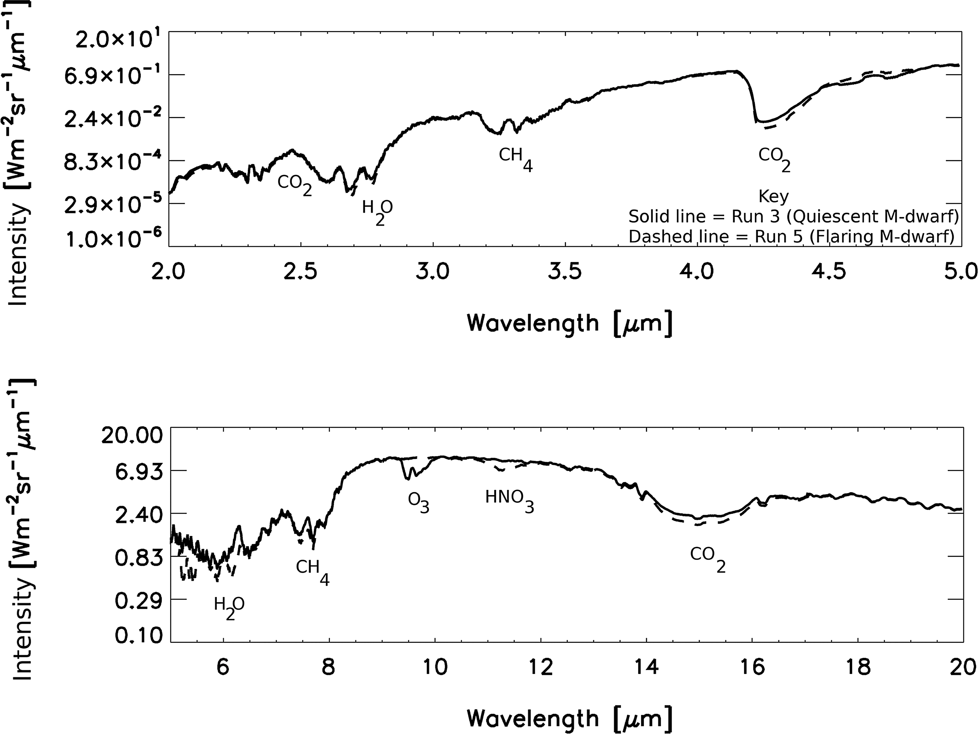
Thermal emission spectra (R _s=100) for run 3 (quiescent M dwarf star) and run 5 (steadily flaring M dwarf star).

4. Discussion and Modeling Caveats

Our main result is that O₃ is removed for strong SCR activity conditions. We now place this result in context by discussing our assumptions and possible responses for Earth-like planets that are difficult to capture in our current model. As mentioned, we assume the upper-limit case where the planet has no magnetic field. Whether our considered planets are indeed tidally locked and the effect on their magnetospheres is currently under debate in the literature and is beyond the scope of the present study.

Ozone 3-D transport effects were discussed earlier (Section 2.1) for Earth. For exoplanets, we now briefly mention some potentially important effects. Critical for the M dwarf cases is the rate of transport of O₃ (produced on the dayside) to the planet's nightside. This will depend, for example, on the atmospheric mass, the day-night temperature gradient, and the planet's rotation rate—hence, its Coriolis force. Seasonal O₃ effects depend on planetary obliquity, eccentricity, or inclination. If the exo-winter is longer than the O₃ photochemical timescales, which are a few weeks on Earth, then O₃ would build up in the exo-winter. Latitudinal transport of O₃ via the “meridional circulation” will be strengthened by exo-orography because this favors atmospheric wave activity, which drives the circulation. Faster planetary rotation will slow the meridional circulation via a strengthened Coriolis force, which disrupts equator-to-pole transport. Since the polar “O₃ hole” on Earth is mainly associated with chlorine released from industrial chlorofluorocarbons, planets with strong emissions of naturally occurring chlorine-containing biomass (e.g., CH₃Cl emitted from seaweed) may feature their own “natural” polar O₃ holes. The altitude dependence of O₃ depends, for example, on the trade-off between (Herzberg-region) UV radiation, which can photolyze O₂ (favoring O₃ at higher altitudes) on the one hand, and the abundance of O₂ (favoring O₃ at lower altitudes) on the other hand. Exoplanets that are more transparent to such UV or/and with thick Earth-like atmospheres may favor a downward shift in the altitude where O₂ photolysis peaks and, hence, since this favors O₃ formation, to a downward shift in their O₃ maximum. O₃ loss via catalytic cycles may also play a role, for example, exoplanets with high lightning activity (hence, high NO_x) or warm, moist water worlds (with high HO_x).

Transport and mixing are important factors for flare-related CR-induced O₃ loss in Earth-like exoplanet scenarios. Critical is how much enhanced NO_x (from CRs) is transported to the planet's O₃ layer. On Earth, high NO formed above the mesosphere (where it is quickly destroyed in lit regions) is transported downward in the dark polar vortex, until it reaches the (lower) stratosphere. At these altitudes, the barrier to mixing at the vortex edge is weaker, and air can escape the vortex to reach sunlit regions at midlatitudes, where considerable O₃ loss occurs.

Eddy-diffusion coefficients (K) are a rather straightforward means in 1-D models to represent the physics of 3-D atmospheric mixing. Patra and Lal (1997) provided a review and suggested global mean K values similar to our work. The quoted range for K in their paper is, however, quite large—more than a factor of 10 depending on latitude and season. As discussed earlier, a test case (run 6) with reduced Eddy mixing still displayed strong O₃ removal of >99%, which suggests that the uncertainties in Eddy mixing do not affect our main conclusions.

Atmospheric mass is another critical quantity that controls, for example, the altitude at which CR shower events peak. We assumed 1 bar surface pressure in all our scenarios. This is, however, currently unconstrained for super-Earths and depends on, for example, delivery, outgassing, and escape processes. Our results for the flaring scenario indicate peak NO production at about 0.1 bar, but we note that a wide range of atmospheric masses are possible. For example, surface pressures of the terrestrial planets in the Solar System range from 10⁻¹⁵ bar on Mercury up to ∼92 bar on Venus.

5. Summary

The scenarios considered the effect of CRs on N₂-O₂ atmospheres with P _surface=1 bar, with mean (day-night averaged) insolation and for a planet (orbiting in the HZ of an M dwarf star) with similar surface gravity and Eddy mixing as Earth. The atmospheric column model used is applied to these rather Earth-like conditions to remain within its range of validity. A future model version will be applied over a much wider range of composition, temperature, and pressure conditions.

Our theoretical spectra calculations suggest that biomarker spectral signals of planets orbiting in the HZ of very active flaring M dwarf stars may show a strong suppression of the O₃ fundamental band (9.6 microns), a deeper CO₂ band (15 microns), and an enhanced H₂O vibrational-rotational band (6.3 microns) compared with less active M dwarf stars. Our work therefore suggests that planets orbiting the HZ of strongly flaring stars may feature low O₃ spectroscopic signals. About 12% of M dwarfs within 7 parsecs have stronger flaring indices than AD Leo, based on (L _X-ray/L _bolometric) measurements by Fleming et al. (1995). Improved catalogues of flaring activity for M stars (as discussed, e.g., in Reiners et al., 2012), as well as improved stellar spectra in the UV and EUV, which could strongly affect calculated O₃ abundances, are desirable.

Surface UVB, a critical quantity for habitability, is low for the M dwarf star cases compared with Earth observations (Table 2) since, for example, the UVB emission of M dwarf stars is weak. Also, the level of UVB atmospheric protection by absorption depends, for example, on the planetary O₃ column. Also, important Rayleigh scatterers in the model affecting UV are N₂, and O₂, whose modeled concentrations are fixed. Biomarkers O₃ and N₂O are generally quite resilient to NO_x-induced photochemical effects from SCRs for Earth-like planets orbiting in the MHZ. O₃, however, may not survive extreme, steady, flaring conditions.

Footnotes

Acknowledgments

This research has been supported by the Helmholtz association through the research alliance “Planetary Evolution and Life.” We are grateful to Prof. James Kasting for providing original code and for useful discussion. P.v.P. acknowledges support from the European Research Council (Starting Grant 209622: E3ARTHs).

Abbreviations

CRPF, Cosmic Ray Proton Flux; CRs, cosmic rays; GCRs, galactic cosmic rays; HZ, habitable zone; MHZ, the habitable zone around an M dwarf star; PAL, proton attenuation length; ppmv, parts per million by volume; RRTM, Rapid Radiative Transfer Module; SCRs, stellar cosmic rays; SPEs, solar proton events; SQuIRRL, Schwarzschild Quadrature InfraRed Radiation Line-by-line; TOA, top-of-atmosphere; vmr, volume mixing ratio; VOCs, volatile organic compounds.

1

The notation following the species name is called the Term Symbol and takes the form^M(2S+1) L, where M is the multiplicity, S is the spin quantum number, and L is the total orbital momentum quantum number. The Term Symbol conveys information about the electronic state of the chemical species considered.

References

Amsler

, Doser

, Antonelli

, Asner

D.M.

, Babu

K.S.

, Baer

, Band

H.R.

, Barnett

R.M.

, Bergren

, Beringer

, Bernardi

, Bertl

, Bichsel

, Biebel

, Bloch

, Blucher

, Blusk

, Cahn

R.N.

, Carena

, Caso

, Ceccucci

, Chakraborty

, Chen

M.-C.

, Chivukula

R.S.

, Cowan

, Dahl

, D'Ambrosio

, Damour

, de Gouvêa

, Degrand

, Dobrescu

, Drees

, Edwards

D.A.

, Eidelman

, Elvira

V.D.

, Erler

, Ezhela

V.V.

, Feng

J.L.

, Fetscher

, Fields

B.D.

, Foster

, Gaisser

T.K.

, Garren

, Gerber

H.-J.

, Gerbier

, Gherghetta

, Giudice

G.F.

, Goodman

, Grab

, Gritsan

A.V.

, Grivaz

J.-F.

, Groom

D.E.

, Grünewald

, Gurtu

, Gutsche

, Haber

H.E.

, Hagiwara

, Hagmann

, Hayes

K.G.

, Hernández-Rey

J.J.

, Hikasa

, Hinchliffe

, Höcker

, Huston

, Igo-Kemenes

, Jackson

J.D.

, Johnson

K.F.

, Junk

, Karlen

, Kayser

, Kirkby

, Klein

S.R.

, Knowles

I.G.

, Kolda

, Kowalewski

R.V.

, Kreitz

, Krusche

, Kuyanov

Yu.V.

, Kwon

, Lahav

, Langacker

, Liddle

, Ligeti

, Lin

C.-J.

, Liss

T.M.

, Littenberg

, Liu

J.C.

, Lugovsky

K.S.

, Lugovsky

S.B.

, Mahlke

, Mangano

M.L.

, Mannel

, Manohar

A.V.

, Marciano

W.J.

, Martin

A.D.

, Masoni

, Milstead

, Miquel

, Mönig

, Murayama

, Nakamura

, Narain

, Nason

, Navas

, Nevski

, Nir

, Olive

K.A.

, Pape

, Patrignani

, Peacock

J.A.

, Piepke

, Punzi

, Quadt

, Raby

, Raffelt

, Ratcliff

B.N.

, Renk

, Richardson

, Roesler

, Rolli

, Romaniouk

, Rosenberg

L.J.

, Rosner

J.L.

, Sachrajda

C.T.

, Sakai

, Sarkar

, Sauli

, Schneider

, Scott

, Seligman

W.G.

, Shaevitz

M.H.

, Sjöstrand

, Smith

J.G.

, Smoot

G.F.

, Spanier

, Spieler

, Stahl

, Stanev

, Stone

S.L.

, Sumiyoshi

, Tanabashi

, Terning

, Titov

, Tkachenko

N.P.

, Törnqvist

N.A.

, Tovey

, Trilling

G.H.

, Trippe

T.G.

, Valencia

, van Bibber

, Vincter

M.G.

, Vogel

, Ward

D.R.

, Watari

, Webber

B.R.

, Weiglein

, Wells

J.D.

, Whalley

, Wheeler

, Wohl

C.G.

, Wolfenstein

, Womersley

, Woody

C.L.

, Workman

R.L.

, Yamamoto

, Yao

W.-M.

, Zenin

O.V.

, Zhang

, Zhu

R.-Y.

, Zyla

P.A.

, Harper

, Lugovsky

V.S.

, Schaffner

2008. Review of particle physics. Phys Lett B, 667:1–6.

Audard

, Guedel

, Kraje

, Kashyap

V.L.

2000. Extreme ultra-violet flare activity in late-type stars. Astrophys J, 541:396–409.

Bichsel

, Groom

D.E.

, Klein

S.R.

2005. Passage of particles through matter. Phys Lett B, 592:853–998.

Brasseur

G.P.

, Orlando

J.J.

, Tyndall

G.S.

1999. Atmospheric Chemistry and Global Change. Oxford University Press: New York.

Chapman

1930. A theory of upper atmosphere ozone. Memoirs of the Royal Meteorological Society, 3:103–125.

COESA (U.S. Committee on Extension to the Standard Atmosphere). 1976. U.S. Standard Atmosphere, 1976, published jointly by the National Oceanic and Atmospheric Administration. the National Aeronautics and Space Administration, and the U.S. Air Force: Washington DC.

Crutzen

P.J.

1970. Influence of nitrogen oxides on atmospheric ozone content. Quarterly Journal of the Royal Meteorological Society, 96:320–325.

Dartnell

L.R.

2011. Ionizing radiation and life. Astrobiology, 11:551–582.

Dwyer

J.R.

2005. The initiation of lightning by runaway air breakdown. Geophys Res Lett, 32:L20808.

10.

Ejzak

L.M.

, Melott

A.L.

, Medvedev

M.V.

, Thomas

B.C.

2007. Terrestrial consequences of spectral and temporal variability in ionizing photon events. Astrophys J, 654:373–384.

11.

Feynman

J.G.

, Gabriel

1988. The effects of high energy particles on planetary missions. Interplanetary Particle Environment. Proceedings of a Conference

Feynman

, Gabriel

JPL publication 88-28, Jet Propulsion Laboratory

Pasadena, CA, 35–47.

12.

Feynman

, Spitale

, Wang

, Gabriel

1993. Interplanetary proton fluence model. J Geophys Res, 98:13281–13294.

13.

Fleming

T.A.

, Schmitt

J.H.M.M.

, Giampa

1995. Correlations of coronal X-ray emission with activity, mass and age of the nearby K and M dwarfs. Astrophys J, 450:401–410.

14.

Gaisser

T.K.

, Hillas

A.M.

1977. Reliability of the method of constant intensity cuts for reconstructing the average development of vertical showers. 15th International Cosmic Ray Conference, Plovdiv, Bulgaria, August 13–26, 1977Conference Papers8. B'lgarska Akademiia na Naukite, Sofia, 353–357.

15.

Gueymard

C.A.

2004. The sun's total and spectral irradiance for solar energy applications and solar radiation models. Solar Energy, 76:423–453.

16.

Gloeckler

, Fisk

L.A.

, Geiss

, Hill

M.E.

, Hamilton

D.C.

, Decker

R.B.

, Krimigis

S.M.

2009. Composition of interstellar neutrals and origin of anomalous cosmic rays. Spa Sci Rev, 143:163–175.

17.

Gopalswamy

2006. Coronal mass ejections of solar cycle 23. Journal of Astrophysics and Astronomy, 27:243–254.

18.

Grenfell

J.L.

, Grießmeier

J.-M.

, Patzer

, Rauer

, Segura

, Stadelmann

, Stracke

, Titz

, von Paris

2007a. Biomarker response to galactic cosmic ray-induced NO_x and the methane greenhouse effect in the atmosphere of an Earthlike planet orbiting an M dwarf star. Astrobiology, 7:208–221.

19.

Grenfell

J.L.

, Stracke

, von Paris

, Patzer

, Titz

, Segura

, Rauer

2007b. The response of atmospheric chemistry on Earthlike planets around F, G, and K stars to small variations in orbital distance. Planet Space Sci, 55:661–671.

20.

Grenfell

J.L.

, Gebauer

, von Paris

, Godolt

, Hedelt

, Patzer

A.B.C.

, Stracke

, Rauer

2011. Sensitivity of biomarkers to changes in chemical emissions in the Earth's Proterozoic atmosphere. Icarus, 211:81–88.

21.

Grießmeier

J.-M.

, Stadelmann

, Motschmann

, Belisheva

N.K.

, Lammer

, Biernat

H.K.

2005. Cosmic ray impact on extrasolar Earth-like planets in close-in habitable zones. Astrobiology, 5:587–603.

22.

Grießmeier

J.-M.

, Stadelmann

, Grenfell

J.L.

, Lammer

, Motschmann

2009. On the protection of extrasolar Earth-like planets around K/M stars against galactic cosmic rays. Icarus, 199:526–535.

23.

Grießmeier

J.-M.

, Khodachenko

, Lammer

, Grenfell

J.L.

, Stadelmann

, Motschmann

2010. Stellar activity and magnetic shielding. Solar and Stellar Variability: Impact on Earth and Planets, Proceedings of the IAU Symposium No. 264

Kosovichev

A.G.

, Andrei

A.H.

, Rozelot

J.-P.

International Astronomical Union

Paris, 385–394.

24.

Güdel

, Audard

, Kashyap

V.L.

, Drake

J.J.

, Guinan

E.F.

2003. Are coronae of magnetically active stars heated by flares? II. Extreme ultraviolet and X-ray flare statistics and the differential emission measure distribution. Astrophys J, 582:423–442.

25.

Haagen-Smit

A.J.

1952. Chemistry and physiology of Los Angeles smog. Ind Eng Chem, 44:1342–1346.

26.

Hamilton

D.C.

1977. The radial transport of energetic solar flare particles from 1 to 6 AU. J Geophys Res, 82:2157–2169.

27.

Hamilton

D.C.

, Mason

G.M.

, McDonald

F.B.

1990. The radial dependence of the peak flux and fluence in solar energetic particle events. Proceedings of the 21st International Cosmic Ray Conference. 5:237–240.

28.

Hauschildt

P.H.

, Allard

, Ferguson

, Baron

, Alexander

D.R.

1999. The NEXGEN model atmosphere grid. II. Spherically symmetric model atmospheres for giant stars with effective temperatures between 3000 and 6800K. Astrophys J, 525:871–880.

29.

Houdebine

E.R.

, Foing

, Rodono

1990. Dynamics of flares on late-type dMe stars. Astron Astrophys, 238:249–255.

30.

Jackman

C.H.

, Frederick

J.E.

, Stolarski

R.S.

1980. Production of odd nitrogen in the stratosphere and mesosphere: an intercomparison of source strengths. J Geophys Res, 85. 10.1029/JC085iC12p07495.

31.

Jackman

C.H.

, Fleming

, Vitt

2000. Influence of extremely large solar proton events in a changing stratosphere. J Geophys Res, 105. 10.1029/2000JD900010.

32.

Jackman

C.H.

, DeLand

M.T.

, Labow

G.J.

, Fleming

E.L.

, Weisenstein

D.K.

, Ko

M.K.W.

, Sinnhuber

, Russell

J.M.

2005. Neutral atmospheric influences of the solar proton events in October–November 2003. J Geophys Res, 110. 10.1029/2004JA010888.

33.

Jackman

C.H.

, Marsh

D.R.

, Vitt

F.M.

, Roble

R.G.

, Randall

C.E.

, Bernath

P.F.

, Funke

, Lopez-Puertez

, Versick

, Stiller

G.P.

, Tylka

A.J.

, Fleming

E.L.

2011. Northern Hemisphere atmospheric influence of the solar proton events and ground level enhancement in January 2005. Atmos Chem Phys, 11:6153–6166.

34.

Khodachenko

M.L.

, Ribas

, Lammer

, Grießmeier

J.-M.

, Leitner

, Selsis

, Eiroa

, Hanslmeier

, Biernat

H.K.

, Farrugia

C.J.

, Rucker

H.O.

2007. Coronal mass ejection (CME) activity of low mass M stars as an important factor for the habitability of terrestrial planets. I: CME impact on expected magnetospheres of Earth-like exoplanets in close-in habitable zones. Astrobiology, 7:167–184.

35.

Kuznetsov

N.V.

, Nymmik

R.A.

, Panasyuk

M.I.

2001. The balance between fluxes of galactic cosmic rays and solar energetic particles, depending on solar activity. In 27th International Cosmic Ray Conference, under the auspices of the International Union of Pure and Applied Physics, 3193.

36.

Kuznetsov

N.V.

, Nymmik

R.A.

, Panasyuk

M.I.

2005. Models of solar energetic particle fluxes: the main requirements and the development prospects. Adv Space Res, 36:2003–2011.

37.

Lammer

, Lichtenegger

H.I.M.

, Kulikov

, Grießmeier

J.-M.

, Terada

, Erkaev

N.V.

, Biernat

H.K.

, Khodachenko

M.L.

, Ribas

, Penz

, Selsis

2007. Coronal mass ejection (CME) activity of low mass M stars as an important factor for the habitability of terrestrial exoplanets. II. CME-induced ion pick-up of Earth-like exoplanets in close-in habitable zones. Astrobiology, 7:185–207.

38.

Lammer

, Kasting

J.F.

, Chassefiere

, Johnson

R.E.

, Kulikov

Y.N.

, Tian

2008. Atmospheric escape and evolution of terrestrial planets satellites. Space Sci Rev, 139:399–436.

39.

Lario

, Marsden

R.G.

, Sanderson

T.R.

, Maksimovic

, Sanahuja

, Balogh

, Forsyth

R.J.

, Lin

R.P.

, Gosling

J.T.

2000. Energetic proton observations at 1 and 5 AU I: January–September 1997. J Geophys Res, 105:18235–18250.

40.

Lario

, Kallenrode

M.-B.

, Decker

R.B.

, Roelof

E.C.

, Krimigis

S.M.

, Aran

, Sanahuja

2006. Radial and longitudinal dependence of solar 4–13 MeV and 27–37 MeV proton peak intensities and fluences: Helios and IMP 8 observations. Astrophys J, 653:1531–1544.

41.

Leggett

S.K.

, Allard

, Berriman

, Dahn

C.C.

, Hauschildt

P.H.

1996. Infrared spectra of low-mass stars: towards a temperature scale for red dwarfs. Astrophys J Suppl Ser, 104:117–143.

42.

Manabe

, Wetherald

R.T.

1967. Thermal equilibrium of the atmosphere with a given distribution of relative humidity. Journal of Atmospheric Sciences, 24:241–259.

43.

Melott

A.L.

, Thomas

B.C.

2011. Astrophysical ionizing radiation and the Earth: a brief review and census of intermittent intense sources. Astrobiology, 11:343–361.

44.

Melsheimer

, Verdes

, Buehler

S.A.

, Emde

, Eriksson

, Feist

D.G.

, Ichzawa

, John

V.O.

, Kasai

, Kopp

, Koulev

, Kuhn

, Lemke

, Ochiai

, Schreier

, Sreerekha

T.H.

, Suzuki

, Takahashi

, Tsujimaru

, Urban

2005. Intercomparison of general purpose clear sky atmospheric radiative transfer models for the millimeter/submillimeter spectral range. Radio Science, 40. 10.1029/2004RS003110.

45.

Mlawer

E.J.

, Taubman

S.J.

, Brown

P.D.

, Iacono

M.J.

, Clough

S.A.

1997. Radiative transfer model for inhomogeneous atmospheres: RRTM, a validated correlated-k model of the longwave. J Geophys Res, 102:16663–16682.

46.

Nicolet

1975. On the production of nitric oxide by cosmic rays in the mesosphere and stratosphere. Planet Space Sci, 23:637–649.

47.

Particle Data Group. 2002. Review of particle physics. Phys Rev D Part Fields, 66:010001.

48.

Patra

P.K.

, Lal

1997. Variability of eddy diffusivity in the stratosphere deduced from vertical distributions of N₂O and CFC-12. Journal of Atmospheric and Solar-Terrestrial Physics, 59:1149–1157.

49.

Pavlov

A.A.

, Kasting

J.F.

2002. Mass-independent fractionation of sulfur isotopes in Archean sediments: strong evidence for an anoxic Archean atmosphere. Astrobiology, 2:27–41.

50.

Pettersen

B.R.

, Hawley

S.L.

1989. A spectroscopic survey of red dwarf flare stars. Astron Astrophys, 217:187–200.

51.

Porter

H.S.

, Jackman

C.H.

, Green

A.E.S.

1976. Efficiencies for production of atomic nitrogen and oxygen by relativistic proton impact in air. J Chem Phys, 65:154–167.

52.

Rauer

, Gebauer

, von Paris

, Cabrera

, Godolt

, Grenfell

J.L.

, Belu

, Selsis

, Hedelt

, Schreier

2011. Biomarkers in super-Earth atmospheres, I. Spectral appearance of super-Earths around M dwarfs. Astron Astrophys, 529. 10.1051/0004-6361/201014368.

53.

Reiners

, Joshi

, Goldman

2012. A catalogue of rotation and activity in early-M stars. Astron J, 143. 10.1088/0004-6256/143/4/93.

54.

Rothman

L.S.

, Jacquemart

, Barbe

, Benner

D.C.

, Birk

, Brown

L.R.

, Carleer

M.R.

, Chackerian

, Chance

, Coudert

L.H.

, Dana

, Devi

V.M.

, Flaud

J.-M.

, Gamache

R.R.

, Goldman

, Hartmann

J.-M.

, Jucks

K.W.

, Maki

A.G.

, Mandin

J.-Y.

, Massie

S.T.

, Orphal

, Perrin

, Rinsland

C.P.

, Smith

M.A.H.

, Tennyson

, Tolchenov

R.N.

, Toth

R.A.

, Vander Auwera

, Varanasi

, Wagner

2005. The HITRAN 2004 molecular spectroscopic database. Journal of Quantitative Spectroscopy and Radiative Transfer, 96:139–204.

55.

Ruzmaikin

, Li

, Zank

, Feynman

, Jun

2005. The radial dependence of solar energetic particle fluxes. Proceedings of the Solar Wind 11 / SOHO 16: Connecting Sun and Heliosphere, ESA SP-592

Fleck

, Zurbuchen

T.H.

, Lacoste

European Space Agency, Noordwijk

the Netherlands, 441–444.

56.

Sander

S.P.

, Finlayson-Pitts

B.J.

, Friedl

R.R.

, Golden

D.M.

, Huie

R.E.

, Kolb

C.E.

, Kurylo

M.J.

, Molina

M.J.

, Moortgat

G.K.

, Orkin

V.L.

, Ravishankara

A.R.

2003. Chemical Kinetics and Photochemical Data for Use in Atmospheric Studies, Evaluation No. 14. Jet Propulsion Laboratory Publication 02-25, Jet Propulsion Laboratory: Pasadena, CA.

57.

Scalo

, Segura

, Fridlund

, Ribas

, Odert

, Leitzinger

, Kulikov

Y.N.

, Grenfell

J.L.

, Rauer

, Kaltenegger

, Khodachenko

M.L.

, Selsis

, Eiora

, Kasting

, Lammer

2007. M type dwarf stars and their relevance for terrestrial planet finding missions. Astrobiology, 7:85–166.

58.

Scherer

, Fichtner

, Stawicki

2002. Shielded by the wind: the influence of the interstellar medium on the environment of Earth. Journal of Atmospheric and Solar-Terrestrial Physics, 64:795–804.

59.

Schreier

, Schimpf

2001. A new efficient line-by-line code for high resolution atmospheric radiation computations incl. derivatives. IRS 2000: Current Problems in Atmospheric Radiation. Smith

W.L.

, Timofeyev

A. Deepak Publishing: Hampton, VA, 381–384.

60.

Segura

, Krelove

, Kasting

J.F.

, Sommerlatt

, Meadows

, Crisp

, Cohen

, Mlawer

2003. Ozone concentrations and ultraviolet fluxes on Earth-like planets around other stars. Astrobiology, 3:689–708.

61.

Segura

, Kasting

J.F.

, Meadows

, Cohen

, Scalo

, Crisp

, Butler

R.A.H.

, Tinetti

2005. Biosignatures from Earth-like planets around M stars. Astrobiology, 5:706–725.

62.

Segura

, Walkowicz

L.M.

, Meadows

, Kasting

J.F.

, Hawley

2010. The effect of a strong stellar flare on the atmospheric chemistry of an Earth-like planet orbiting an M dwarf. Astrobiology, 10:751–771.

63.

Seo

E.S.

, Ormes

J.F.

, Streitmatter

R.E.

, Stochaj

S.J.

, Jones

W.V.

, Stephens

S.A.

, Bowen

1991. Measurement of cosmic ray proton and helium spectra during the 1987 solar minimum. Astrophys J, 378:763–772.

64.

Shao

, Lu

S.H.

, Liu

, Xie

, Chang

C.C.

, Hunag

, Chen

Z.M.

2009. Volatile organic compounds measured in summer in Beijing and their role in ground-level ozone formation. J Geophys Res, 114. 10.1029/2008JD010863.

65.

Smart

D.F.

, Shea

M.A.

2002. A review of solar proton events during the 22^nd solar cycle. Adv Space Res, 30:1033–1044.

66.

Svensmark

, Christensen

E.F.

1997. Variation of cosmic ray flux and global cloud coverage—a missing link in solar-climate relationships. Journal of Atmospheric and Solar-Terrestrial Physics, 59:1225–1232.

67.

Tarduno

, Cottrell

R.D.

, Watkeys

M.K.

, Hofmann

, Doubrovine

P.V.

, Mamajek

E.E.

, Liu

, Sibeck

D.G.

, Neukirch

L.P.

, Usui

2010. Geodynamo, solar wind, and magnetopause 3.4 to 3.45 billion years ago. Science, 327:1238–1240.

68.

Thomas

B.C.

, Jackman

C.H.

, Melott

A.L.

, Laird

C.M.

, Stolarski

R.S.

, Gehrels

, Cannizo

J.K.

, Hogan

D.P.

2005a. Terrestrial ozone depletion due to a Milky Way gamma ray burst. Astrophys J, 622:L153–L156.

69.

Thomas

B.C.

, Melott

A.L.

, Jackman

C.H.

, Laird

C.M.

, Medvedev

M.V.

, Stolarski

R.S.

, Gehrels

, Cannizzo

J.K.

, Hogan

D.P.

, Ejzak

L.M.

2005b. Gamma ray bursts and the Earth: exploration of atmospheric, biological, climatic and biogeochemical effects. Astrophys J, 634:509–533.

70.

Vardavas

I.M.

, Carver

J.H.

1984. Solar and terrestrial parameterizations for radiative-convective models. Planet Space Sci, 32:1307–1325.

71.

von Clarmann

, Höpfner

, Funke

, López-Puertes

, Dudhia

, Jay

, Schreier

, Ridolfi

, Cecherini

, Kerridge

B.J.

, Reburn

, Siddans

2002. Modelling of atmospheric mid-infrared radiative transfer: the AMIL2DA algorithm intercomparison experiment. Journal of Quantitative Spectroscopy and Radiative Transfer, 78:381–407.

72.

Wang

, Li

, Cihlar

, Wardle

D.I.

, Kerr

2000. Validation of an UV inversion algorithm using satellite and surface measurements. J Geophys Res, 105:5037–5048.

73.

WMO. 1994. Scientific Assessment of Ozone DepletionReport Number 37World Meteorological Organization (WMO): Geneva, Switzerland.

74.

Ziegler

J.F.

1996. Terrestrial cosmic rays. IBM Journal of Research and Development, 40:19–39.

Response of Atmospheric Biomarkers to NO x -Induced Photochemistry Generated by Stellar Cosmic Rays for Earth-like Planets in the Habitable Zone of M Dwarf Stars

Abstract

1. Introduction

1.1. Cosmic rays (CRs) and magnetic fields

1.2. Interactions of CRs with atmospheres and biomarkers

2. Description of Model Approach, Model, and Runs

Model approach

2.1. Coupled climate-chemistry atmospheric column model

The climate module is a global-mean stationary, hydrostatic column model of the atmosphere

The chemistry module was described by Pavlov and Kasting et al. (2002)

The cosmic ray scheme

2.2. Theoretical line-by-line spectral model

2.3. Application of a stationary SCR model to active M dwarf star conditions

Biomarker photochemical timescales

AD Leo variability timescales

Diurnal O3 observations on Earth

2.4. About the runs

Cosmic ray input data for the runs

3. Results

3.1. Top-of-atmosphere CR energy spectra and nitrogen monoxide (NO) production

3.2. Column amounts of biomarkers and related compounds

3.3. Atmospheric profiles of biomarkers and related compounds

3.4. Atmospheric temperature profiles

3.5. Thermal emission spectra

4. Discussion and Modeling Caveats

5. Summary

Footnotes

Acknowledgments

Abbreviations

1

References

Diurnal O₃ observations on Earth