The Carbonate-Silicate Cycle and CO 2 /Climate Feedbacks on Tidally Locked Terrestrial Planets

2.1. Model description

For this study, we used the GENESIS version 3.0 GCM (Alder et al., 2011), which has updated CO₂ absorption coefficients and atmospheric radiative transfer treatments from CCM3 (Kiehl et al., 1998), as compared to GENESIS version 2.3 in Paper 1. These updated absorption coefficients allow for the atmospheric CO₂ concentrations to be varied over a much greater range, from 0 to 0.1 bars, without impacting the accuracy of the radiative transfer calculations. The GENESIS GCM consists of a spectral atmospheric general circulation model coupled to multilayer surface models of vegetation, soil, snow, ice, and ocean (Thompson and Pollard, 1997; Alder et al., 2011). The GCM grid for this study is spectral T31 resolution (∼3.75°), for both the atmosphere and surface models.

The multilayer soil model (Pollard and Thompson, 1995) extends from the surface to a depth of 4.25 m, with layer thicknesses increasing from 5 cm at the top to 2.5 m at the bottom. Vertical diffusion of heat and soil moisture are included, with diffusion coefficients depending on soil texture and moisture. For this study, the soil is assumed to consist of 33% sand, 33% silt, and 33% clay. The surface module also includes a 50 m slab ocean. This ocean does not circulate but includes linear horizontal heat diffusion, with the coefficient chosen to best fit modern Earth climate. Any sea ice that forms is advected by atmospheric surface winds. The atmospheric model predicts water vapor, cloud amounts, precipitation, and surface evaporation, and the land surface models include variable soil moisture, soil ice, and snow cover. The standard GENESIS v3.0 GCM was adapted for this study by adding the ability (i) to set the inertial rotation rate in the Coriolis terms for atmospheric and sea-ice dynamics, (ii) to set the day length for solar radiation, including an option for no temporal variation (tidal locking), and (iii) optionally to initialize the atmosphere and soil to completely dry conditions.

2.2. Atmospheric constituents

For all our simulations, the concentrations of trace greenhouse gases other than CO₂ were set to present Earth levels: CH₄ 1.7 ppmv, N₂O 0.31 ppm, CFC₁₁ 0.28 pptv, and CFC₁₂ 0.50 ppt. This choice of parameters was made to allow for the closest comparison between present Earth weathering rates and those of the model planets. The water vapor concentration is determined by the model. The atmospheric carbon dioxide concentration was set to 355 ppm for the control simulations, described first, and was then varied over wide ranges in binary searches with interactive carbonate-silicate cycle simulations.

2.3. Geography and weathering rates

The surface topography used for this study was the present Earth land and ocean distribution scaled to T31 resolution (∼3.75°). We used an Earth-like distribution of continent and ocean areas to illustrate the fact that the silicate weathering rate is affected by both the total land area coverage and their geographic distribution. Comparable knowledge of extrasolar planets will likely not be available in the next few decades, if ever. That said, fractional land-ocean coverage may eventually be obtained from color photometry of such planets (Cowan et al., 2009), so somewhat cruder models of the type described here could eventually be applied to them.

For the variable CO₂ simulations, we used a standard binary-search algorithm to find the CO₂ concentration that balances the carbonate-silicate cycle for a given solar insolation and substellar point. Each search was initiated by performing a pair of GCM simulations with extreme CO₂ amounts of 1 ppm and 1,000,000 ppm, bracketing all possible final values, and performing a third simulation with the “current” CO₂ amount set to the geometric mean of 1 ppm and 1,000,000 ppm, that is, (1×1,000,000)^1/2, to allow for the logarithmic effect of CO₂ on radiative fluxes. Each GCM simulation with a given CO₂ amount was run for 10 Earth years, and the final average (here and elsewhere, annual averages are taken over the last 365 concurrent Earth days of the simulation) surface air temperature and runoff distribution was used to calculate silicate weathering rates using Eq. 1 below. The CO₂ outgassed from volcanoes is set to the present Earth value of 6.8×10¹² mol C/year (Donnadieu et al., 2006). Land areas that have average surface temperatures between 0°C and 35°C are assumed to weather at the ambient surface temperature. Any land below 0°C is assumed to have zero runoff and, hence, zero weathering. Any land for which the local average surface temperature is above 35°C is assumed to have the same weathering rate as land at 35°C. This qualification ensures that the land will not weather chemically faster than it can weather physically. (Tropical soils today are already heavily chemically weathered, which suggests that physical weathering becomes limiting at surface temperatures at or below those in the present tropics.) Then, the CO₂ output from the volcanoes (which is set to a constant) and the CO₂ drawdown rate (calculated from the surface temperature and runoff) are compared. The CO₂ weathering rate is calculated from the following equation, modified from Walker et al. (1981): \documentclass{aastex}\usepackage{amsbsy}\usepackage{amsfonts}\usepackage{amssymb}\usepackage{bm}\usepackage{mathrsfs}\usepackage{pifont}\usepackage{stmaryrd}\usepackage{textcomp}\usepackage{portland, xspace}\usepackage{amsmath, amsxtra}\pagestyle{empty}\DeclareMathSizes{10}{9}{7}{6}\begin{document} \begin{align*} \frac {d {\rm CO} _2} {dt} = \frac {1} {2} \int_ {- 90} ^ {90} \int_ {180^ {\circ} {\rm E}} ^ {180^ {\circ} {\rm W}} S \left(\frac {[{\rm CO} _2]} {[{\rm CO} _2] _0} \right) ^ {0.3} \left({\frac {\rm runoff} {\rm runoff} _0} \right) e \frac {T - T_0} {17.7} dA \tag {1} \end{align*} \end{document}

Here, S (8.4543×10⁻¹⁰ C s⁻¹ m⁻²) is the present Earth silicate weathering rate per unit area; runoff is the annual mean runoff rate at a grid point; dA represents the surface area in a grid box that is weatherable; T is the annual mean surface air temperature at a grid point; T ₀ is the reference temperature for the silicate weathering rate (here, 288 K); [CO₂] is the atmospheric concentration of carbon dioxide; runoff₀ is a reference globally averaged runoff amount (0.665 mm d⁻¹) determined from running GENESIS under present Earth conditions; and [CO₂]₀ is the CO₂ concentration (355 ppm) used for determining the reference runoff amount. The global integral of the product is halved because only half the CO₂ used in the reaction goes into carbonates, while the rest is lost back to the atmosphere when calcium carbonate is precipitated. In the exponential, the 17.7 appearing in the denominator is the approximate Arrhenius temperature dependence for the dissolution of albite and adularia. Busenberg and Clemency (1976) showed “that calcium-bearing silicate minerals exhibit the same dissolution kinetics as sodium and potassium silicates as a function of time.” So, this temperature dependence for silicate weathering was adopted by Walker et al. (1981) and by us. If outgassing is greater than weathering, the CO₂ concentration for the next GCM simulation is chosen to be the geometric mean of the current value and the high value of the previous bracketing pair, and the current value becomes the new lower member of the pair. Conversely, if outgassing is less than weathering, the next CO₂ concentration is chosen to be the geometric mean of the current value and the low value of the previous bracketing pair, and the current value becomes the new upper member of the pair (i.e., a standard binary search). When the change in CO₂ between one run and the next is less than 10% of the previous value, we conclude that the carbonate silicate cycle is nearly balanced, and so we have found the equilibrium CO₂ level for that configuration.

2.4. Numerical experiments

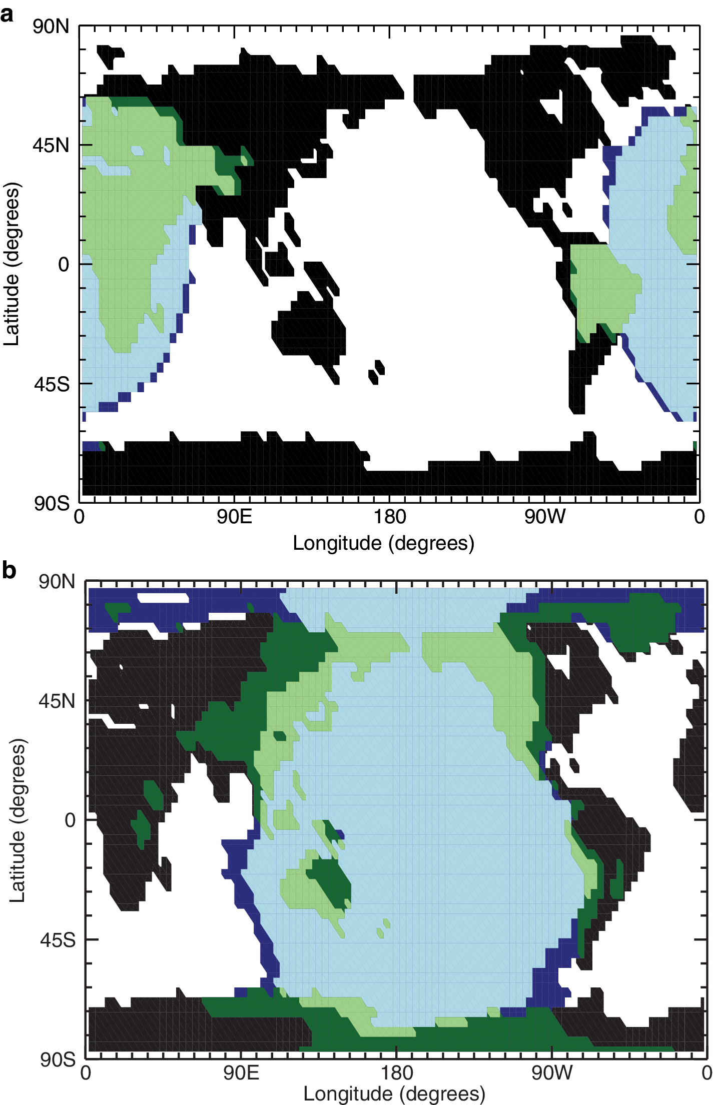
We performed a suite of experiments with tidal locking and perfectly circular orbits, and a constant orbital period of 240 h (10 days). The 240 h orbital period was chosen for comparison with the work of Joshi (2003). In that paper, the planets were in one of three configurations: land covered, water covered, and half-land, half-water (Northern Continent configuration). In the present study, we extended the configurations to the present Earth continental distribution to examine the role of continentality in weather patterns and habitability. Two different substellar points were chosen, one at 0° latitude and 0° longitude (hereafter referred to as the Atlantic Basin simulation) (Fig. 1a) and the other at 0° latitude and 180° longitude (hereafter referred to as the Pacific Basin simulation) (Fig. 1b). The top-of-atmosphere solar insolation was set equal to that of present Earth (1365 W m⁻²). As control runs, a tidally locked planet with an invariant atmospheric CO₂ concentration of 355 ppm was chosen for each of the two substellar points. Both control simulations were spun up from rest and integrated for 10 years. For these simulations, the solar spectrum was used, as opposed to the spectra of the appropriate M star. This was done to isolate the changes in the simulations to just the substellar points while maintaining the capability of comparison with present Earth temperatures.

OPEN IN VIEWER

FIG. 1.

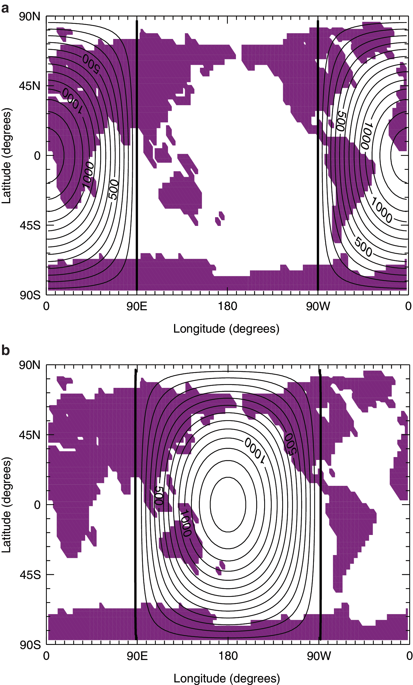
The distribution of insolation for the (a) Atlantic Basin simulation and (b) Pacific Basin simulation. The contour interval is 100 W m⁻². Color images available online at www.liebertonline.com/ast

3.1. Constant CO₂ simulations

For both the Atlantic Basin simulation and the Pacific Basin simulation, the upper-level atmospheric circulations resemble the 240 h orbiter simulations for both the dry planet and the aquaplanet of Paper 1. Those atmospheres showed a strong westerly equatorial jet stream with a central area of low pressure on the sunlit side that corresponded to the location of the substellar point and two high-pressure vortices on the dark side near 60° latitude. So the overall circulation is not affected greatly by the presence of topography. However, some small stationary Rossby waves are seen in mountainous areas over the continents.

Figure 2 shows the mean annual surface temperature for both the Atlantic Basin simulation (Fig. 2a) and the Pacific Basin simulation (Fig. 2b). In Paper 1, the area with mean surface temperatures between 0°C and 50°C was a circular region centered on the subsolar point. Here, because of the topography, this region is not entirely circular; however, the basic geometry of the habitable region is similar. Also, in Paper 1, the lowest surface temperatures were collocated with the upper-level vortices in both the dry planet and the aquaplanet cases (−117°C and −62°C, respectively). The current simulations show that the temperature distribution depends on the topography below the vortices. In the Atlantic Basin simulation, the coldest temperature in the Northern Hemisphere (−63°C) is located west of the Northern Hemisphere vortex near Kamchatka. In the Pacific Basin simulation, the coldest temperature (−36°C) is located in Europe. In Paper 1, the hottest temperatures for both the dry planet and the aquaplanet were located at the substellar point (80°C and 40°C for dry planet and aquaplanet runs, respectively). In the Atlantic Basin simulation shown here, the hottest temperature (41°C) is in South America, not at the substellar point. This shift westward from the substellar point is caused by the lack of water vapor in the air coming over the Andes from the unlit side of the planet. This prevents clouds from forming over South America and thereby allows the stellar insolation to penetrate to the surface. The substellar point is located over the Atlantic Ocean, which allows water to evaporate and form clouds that block the incoming stellar insolation. In the Pacific Basin simulation, the hottest surface temperature is in Australia (44°C), not at the substellar point. Again, the surface temperatures are hottest over land areas, although in this case there are no mountains near the substellar point to further decrease the water vapor. Both the Atlantic Basin and Pacific Basin cases have average temperatures (254 and 260 K, respectively) between that dry planet and aquaplanet from Paper 1 (242 and 268 K, respectively). Even though these planets more closely resemble present Earth than the planets in Paper 1, the simulations are still significantly colder than present Earth. This difference in average surface temperature between the control planets and present Earth is due to the higher planetary albedos in the control planets. The higher albedos are a result of the cloud reflection from the substellar point updraft. Although the surface features in these two simulations are different from both the dry planet and the aquaplanet cases previously studied, the atmospheric circulations closely resemble those cases. Some minor differences are present: the contoured 200 hPa geopotential heights and the 200 hPa wind vectors show topographically forced waves from the landforms present (not shown). Specifically, the location of the Andes and the Rocky Mountains can be seen as waves in the upper levels over South America and North America. Also, there are waves in the vortices in the Southern Hemisphere as the contours cross from ocean to land near Antarctica. In the Pacific Basin simulation, waves can be seen over South America and North America, respectively, in both simulations. Also in both simulations, waves may be seen over Asia, denoting the presence of the Himalayas.

OPEN IN VIEWER

FIG. 2.

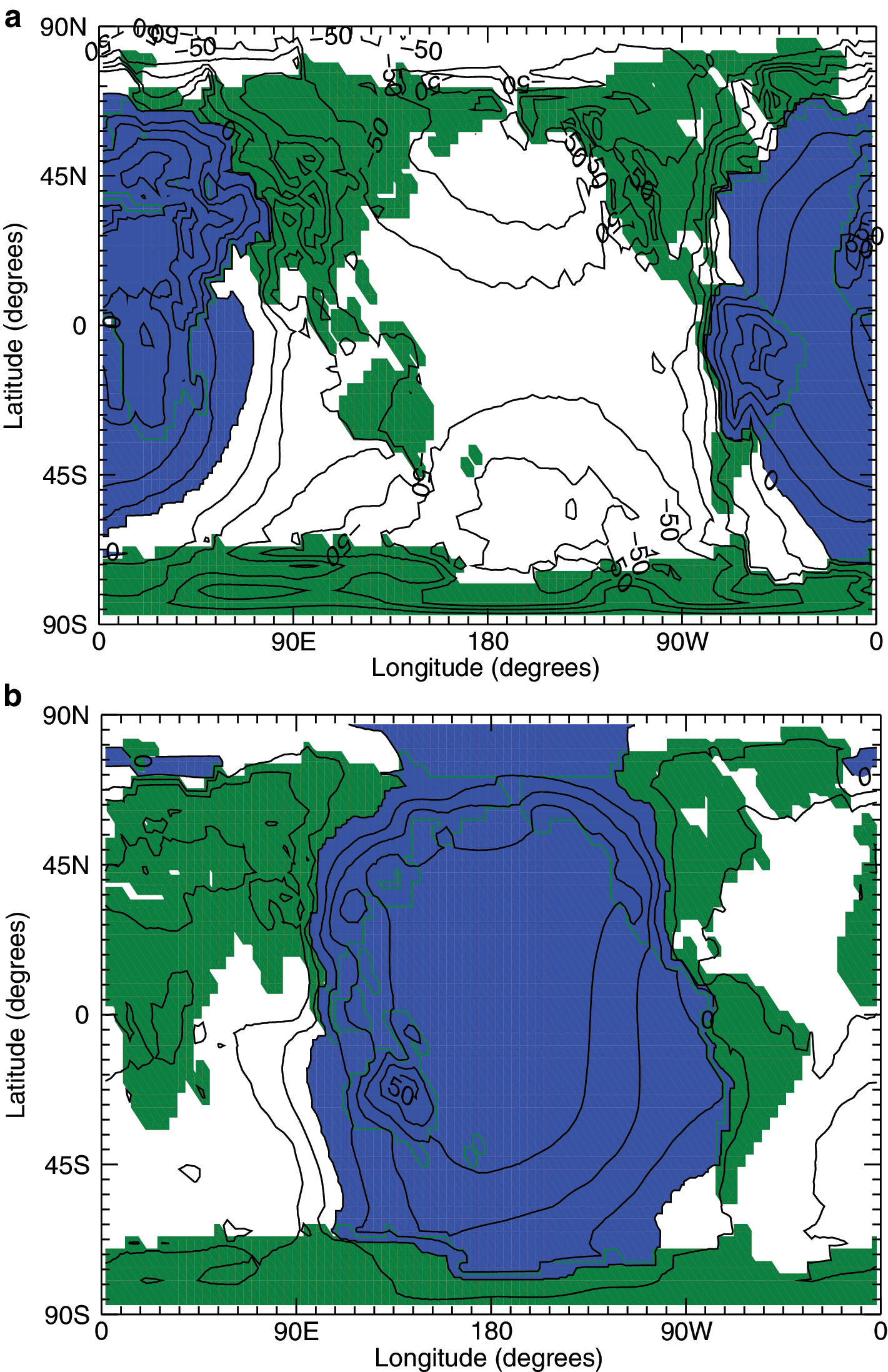
The average annual GCM surface air temperatures for (a) the Atlantic Basin simulation and (b) the Pacific Basin simulation, with control amounts of CO₂ (355 ppm). The contour interval is 10°C with blue shading denoting regions with temperatures between 0°C and 50°C. The green areas denote the location of land masses in the simulation. Land masses are outlined in the blue area. Note that the mountainous areas near the terminator are more likely to be warm than are surrounding land and water. Color images available online at www.liebertonline.com/ast

Comparing the Pacific Basin case with the Atlantic Basin case, the different availability of open ocean for evaporation and latent heat transport to the dark side of the planet can be seen in the difference in the low temperatures. The Pacific Basin case, with its greater expanse of open water, has more potential for latent heat transport to the dark side of the planet, which increases the average surface temperature. In the Atlantic Basin case, the transport is much less than in the Pacific Basin case, lowering the average surface temperature.

For each simulation, the Habitable Area (HA), the Continuously Habitable Area (CHA), the Land Habitable Area (LHA), and the Land Continuously Habitable Area (LCHA) are calculated. The HA is defined as the surface area where the average surface temperature is greater than or equal to 0°C and less than or equal to 50°C. This corresponds to temperate areas on present Earth where only hardier organisms may reside. The LHA is the part of the HA that includes land. The CHA is the surface area where the minimum temperature is greater than or equal to 0°C and the maximum temperature is less than or equal to 50°C. This corresponds to the tropical areas of present Earth where many organisms can readily survive. Areas in the LCHA include continental tropical climes that are ideal for the development of animal life and civilizations. If civilizations were to develop in these warm areas, they could spread to the LHA. The 50°C constraint was suggested by Ward and Brownlee (2000) as the limit for multicellular life. This seems like a reasonable estimate. Tansey and Brock (1972) showed that eukaryotic life in general can survive at temperatures up to 60°C, but the high end of this range applies to fungi, not to plants and animals. Like Ward and Brownlee, we are interested in the latter organisms here. As may be seen in Table 1, although the temperatures are warmer in the Pacific Basin case, the HA and CHA are quite similar between the two cases. Even more interesting is that the Pacific Basin case has less total habitable land area (LHA and LCHA) than the Atlantic Basin case. This difference is due to the lack of sunlight reaching exposed land areas in the Pacific Basin case. So even though the Pacific Basin case is warmer overall, the amount of habitable land surface area is smaller than that in the Atlantic Basin case. As can be seen in Fig. 3, some of the HA is located on the dark side of the planet. Although these locations are not viable for photoautotrophs (like green plants on Earth), these temperate locations could be viable for chemoautotrophic multicellular life-forms. The Atlantic Basin case planetary albedo is slightly lower than the Pacific Basin case due to the lack of large continents on the starlit side of the planet in the Pacific Basin case. Even though much of the planets' surfaces are below the freezing point of water, these areas are most prevalent on the nightside of the planet, which keeps these ice-covered areas from affecting the albedo.

OPEN IN VIEWER

FIG. 3.

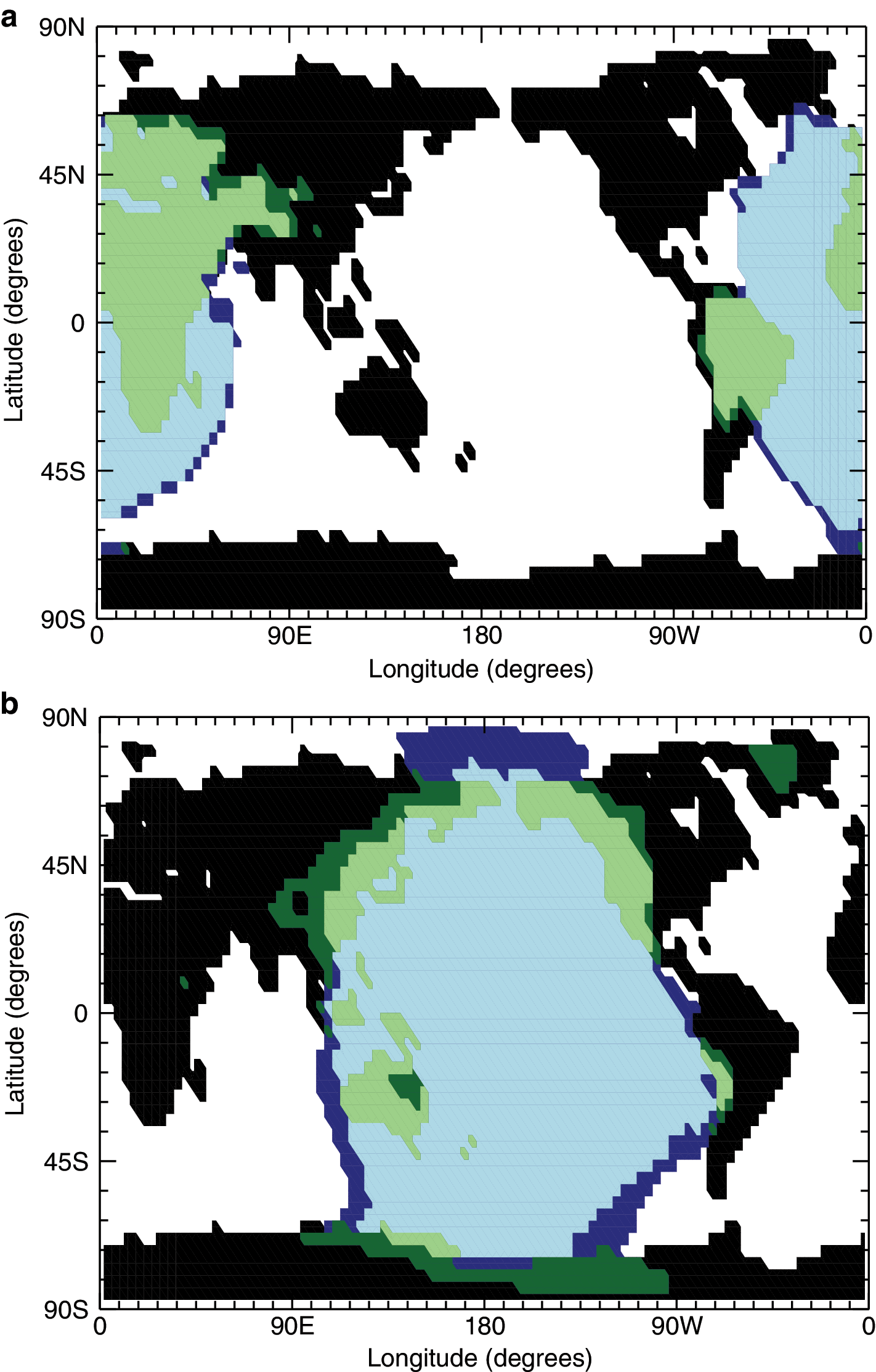
The HA (dark blue), the CHA (light blue), the LHA (dark green), and the LCHA (light green) for the (a) Atlantic Basin simulation and the (b) Pacific Basin simulation. These results are for the fixed 355 ppm CO₂ simulations. The acronyms refer to different definitions of the habitable zone, as defined in the text. Black areas denote continental areas that are inhospitable, and white areas denote frozen ocean areas. Areas that are in the LHA, CHA, and LCHA are also in the total HA. Areas in the LCHA are also in the total LHA and total CHA. Color images available online at www.liebertonline.com/ast

3.2. Variable CO₂ simulations

We next performed a series of simulations in which we balanced the carbonate-silicate cycle, expressed by Eq. 1, by iteratively adjusting atmospheric CO₂. In the Atlantic Basin simulation, the carbonate-silicate cycle balanced at a CO₂ concentration between 7 and 12 ppm. The simulation shown here corresponds to a CO₂ concentration of 7 ppm. This is only ∼2% of present Earth atmospheric concentration. This level of atmospheric carbon dioxide is below the limit at which terrestrial plants can photosynthesize [10 ppm CO₂ for the hardiest C₄ plants (Caldeira and Kasting, 1992)]; hence, this planet would be uninhabitable for any photosynthetic life present on Earth today. The reason the CO₂ concentration is so low is because the substellar point is over the Atlantic Basin (Fig. 1a). With the substellar point in this location, a large amount of land area is illuminated, and consequently surface temperatures and weathering rates are very high. Note that major mountain ranges, like the Himalayas and the Andes, are illuminated in this simulation. The insolation warms the surface such that when it rains the silicate rocks are easily weathered, which draws down the CO₂ concentration in the atmosphere.

In the Pacific Basin simulation, by contrast, the carbonate-silicate cycle balanced at a CO₂ concentration between 59,068 ppm and 60,311 ppm, which corresponds to a CO₂ partial pressure of ∼0.060 bar. The actual CO₂ concentration in this simulation is 60,311 ppm. This is nearly 200 times higher than the atmospheric CO₂ concentration on present Earth. The reason is that the substellar point is over the middle of the Pacific Ocean, so there is little continental landmass in the region where the solar insolation is high (as seen in Fig. 1b). This lack of landmass leads to a need for larger atmospheric CO₂ concentrations to keep the landmasses on the dark side of the planet warm enough for rain to fall there and to thereby weather the continents. In reality, the atmospheric CO₂ concentration on a planet like this one might be limited by seafloor weathering, rather than by continental weathering (Sleep and Zahnle, 2001), so the CO₂ partial pressure calculated here may be too high. Quantifying this effect is difficult, though. The present calculations simply show that the same tidally locked planet could end up with greatly different atmospheric CO₂ concentrations, depending on which side of the planet is sunlit.

The annually averaged surface temperature fields for these variable-CO₂ simulations are shown in Fig. 4a, 4b. Areas in blue have average temperatures above 0°C, which makes these areas more likely to have liquid water present. The locations of the warmest and coldest areas on each planet are approximately the same for these planets and their respective controls, discussed above. However, the global average surface temperatures and the global temperature ranges are different (Table 1). The Atlantic Basin simulation was significantly cooler on a global average (7°) than the control run, largely as a result of its much lower CO₂ concentration and smaller greenhouse effect. As a consequence of the lowered temperatures, the HA, CHA, LHA, and LCHA all decreased, but not drastically. By contrast, the Pacific Basin simulation was much hotter than the corresponding control run (21°) because of its very high CO₂ concentration and large greenhouse effect. The amount of habitable surface area increased in all categories except temperature range when compared to the 355 ppm control simulation. The warmer temperatures are especially evident on the dark side of the planet, where the lowest temperatures are much higher (−16°C) than in any of the other simulations (−36°C for the warmest of the other cases). This can be seen as a lack of isotherms on the unlit portion of the planet in Fig. 4b when compared with Fig. 4a. The temperature range decreased because the increased greenhouse effect (or, equivalently, the increased radiative time constant of the atmosphere) allowed warm air to be advected around to the dark side of the planet without cooling as much. Because of the increased temperatures, the HA, CHA, LHA, and LCHA all increased, with the LCHA and LHA doubling compared to the fixed-CO₂ simulation (Table 1).

OPEN IN VIEWER

FIG. 4.

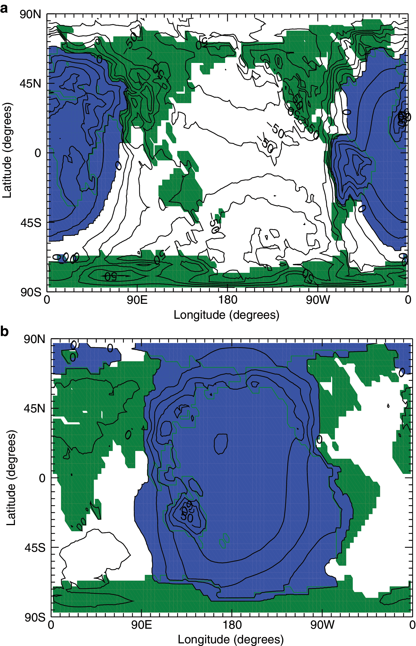
The average annual surface air temperature in degrees Celsius for the (a) Atlantic Basin simulation and the (b) Pacific Basin simulation. These are for the binary-search equilibrated-CO₂ simulations with CO₂=7 ppm in panel (a) and 60,311 ppm (0.06 bar) in panel (b). The contour interval is 10°C with blue shading denoting regions with temperatures between 0°C and 50°C. The green areas denote the location of land masses in the simulation. Land masses are outlined in the blue area. Color images available online at www.liebertonline.com/ast

The HA, CHA, LHA, and LCHA are shown in Fig. 5a, 5b for their respective simulations. For the Atlantic Basin simulation, the HA, CHA, LHA, and LCHA have all decreased compared to the control. Notable differences include the Northern Atlantic Ocean, the HA on the South American continent, and the Ural Mountains on the Eurasian continent. For the Pacific Basin simulation, the HA, CHA, LHA, and LCHA have all increased compared to the control. The HA expands to include all of Australia (where only a portion of the continent was habitable in the Atlantic Basin simulation) and much larger chunks of the Eurasian, North American, and South American continents. The Antarctic and Arctic regions also become partially habitable. Even Africa, which is nearly at the antistellar point, gains some habitability.

OPEN IN VIEWER

FIG. 5.

The HA (dark blue), the CHA (light blue), the LHA (dark green), and the LCHA (light green) for the (a) Atlantic Basin simulation (7 ppm CO₂) and the (b) Pacific Basin simulation (60,311 ppm CO₂). Black areas denote continental areas that are inhospitable, and white areas denote frozen ocean areas. Areas that are in the LHA, CHA, and LCHA are also in the total HA. Areas in the LCHA are also in the total LHA and total CHA. Color images available online at www.liebertonline.com/ast

Although the calculations shown here were all done at 1 AU equivalent distance from the star (i.e., present Earth insolation), the conclusions can be generalized to planets orbiting elsewhere within the habitable zone of their parent star. The farther away a planet is from its star, the higher atmospheric CO₂ would need to be to balance the carbonate-silicate cycle (assuming Earth-like rates of volcanism). High atmospheric CO₂ tends to moderate surface temperatures around the planet by increasing the radiative time constant of the atmosphere. So, if all other factors are equal, a tidally locked planet orbiting near the outer edge of the habitable zone should be more temperate than a planet orbiting near the inner edge. Conversely, larger planets, with more active volcanism, should have higher CO₂ partial pressures and higher mean surface temperatures than similarly located Earth-sized planets. Provided they are not too hot on their daysides, such large planets should also have warmer nightsides and greater habitable areas than smaller planets.