Giant Polygons and Mounds in the Lowlands of Mars: Signatures of an Ancient Ocean?

Abstract

This paper presents the hypothesis that the well-known giant polygons and bright mounds of the martian lowlands may be related to a common process—a process of fluid expulsion that results from burial of fine-grained sediments beneath a body of water. Specifically, we hypothesize that giant polygons and mounds in Chryse and Acidalia Planitiae are analogous to kilometer-scale polygons and mud volcanoes in terrestrial, marine basins and that the co-occurrence of masses of these features in Chryse and Acidalia may be the signature of sedimentary processes in an ancient martian ocean.

We base this hypothesis on recent data from both Earth and Mars. On Earth, 3-D seismic data illustrate kilometer-scale polygons that may be analogous to the giant polygons on Mars. The terrestrial polygons form in fine-grained sediments that have been deposited and buried in passive-margin, marine settings. These polygons are thought to result from compaction/dewatering, and they are commonly associated with fluid expulsion features, such as mud volcanoes. On Mars, in Chryse and Acidalia Planitiae, orbital data demonstrate that giant polygons and mounds have overlapping spatial distributions. There, each set of features occurs within a geological setting that is seemingly analogous to that of the terrestrial, kilometer-scale polygons (broad basin of deposition, predicted fine-grained sediments, and lack of significant horizontal stress). Regionally, the martian polygons and mounds both show a correlation to elevation, as if their formation were related to past water levels. Although these observations are based on older data with incomplete coverage, a similar correlation to elevation has been established in one local area studied in detail with newer higher-resolution data.

Further mapping with the latest data sets should more clearly elucidate the relationship(s) of the polygons and mounds to elevation over the entire Chryse-Acidalia region and thereby provide more insight into this hypothesis. Key Words: Mars—Ocean—Giant polygons—Mounds—Lowlands—Chryse—Acidalia—Mud volcano. Astrobiology 12, 601–615.

1. Introduction

T he fundamental question of whether an ocean ever existed on Mars remains controversial. Some consider that major portions of the lowlands were covered by an ocean or standing bodies of water at times in the early history of the planet (Parker et al., 1989, 1993; Baker et al., 1991; Scott et al., 1991, 1995; Rice and Edgett, 1997; Head et al., 1998, 1999; Clifford and Parker, 2001; Kreslavsky and Head, 2002; Fairén et al., 2003; Boyce et al., 2005; Dohm et al., 2008; Di Achille and Hynek, 2010; McGowan, 2010). Others question interpretations of landforms speculated to be shorelines, though these authors have noted that a lack of recognizable shorelines would not preclude there having once been a martian ocean (Tanaka, 1997; Malin and Edgett, 1999, 2001; Tanaka et al., 2003; Ghatan and Zimbelman, 2006). And some comment that HiRISE images fail to show high-latitude, fine-grained sediments that might be expected for offshore settings (McEwen et al., 2007).

Many parts of the martian lowlands that are speculated to have been sites of water bodies are also characterized by extensive networks of giant polygons and masses of bright mounds. These features have been studied for decades, but their origins are still debated. Earlier studies tended to address either the polygons or the mounds separately. In this paper, we consider both polygons and mounds and suggest that the two sets of features could be linked. We focus on the Chryse-Acidalia portion of the lowlands (Fig. 1), where giant polygons and mounds are abundant and widespread, and we provide recent data from Mars and Earth that may provide new insights into the origin(s) of these martian features.

FIG. 1.

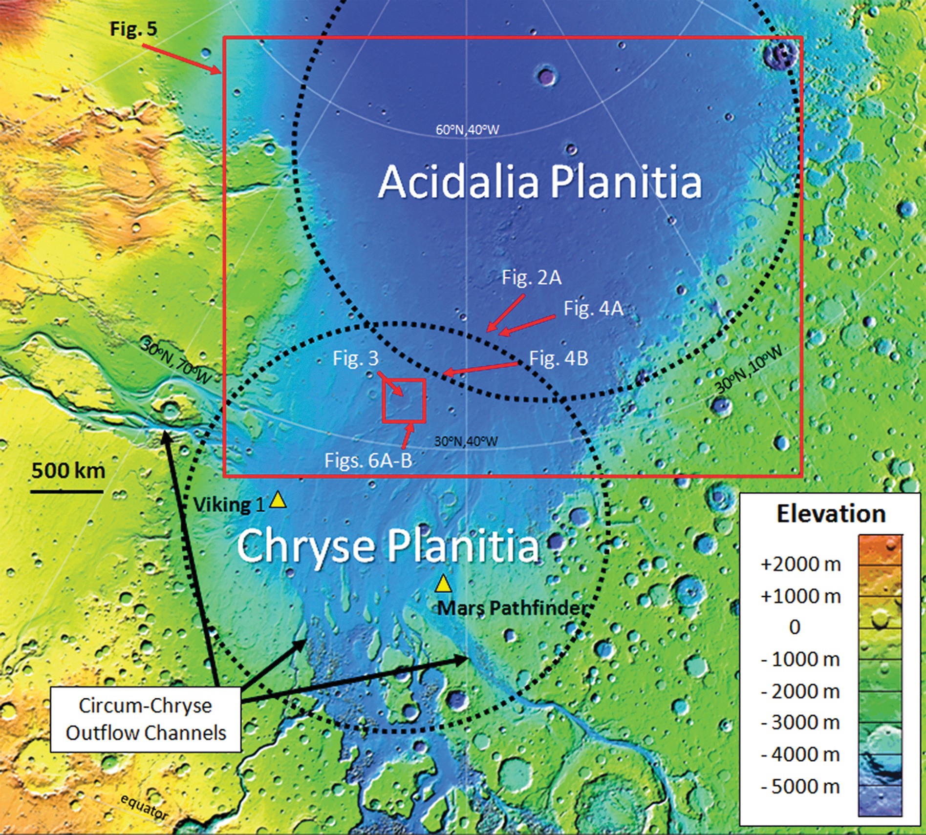
Location map. Elevation base map (polar projection) from full resolution, Mars Orbital Laser Altimeter (MOLA) data. Locations shown for Figs. 2A, 3, 4A, 4B, 5, and 6A, 6B. Dashed circle and portion of the circle show approximate outlines of the Chryse and Acidalia impact basins, as determined by Frey (2006, 2008) from mapping of quasi-circular depressions.

2. Methods/Data Sets

To study spatial distributions for this paper, we combined image data from the Context (CTX) camera on NASA's Mars Reconnaissance Orbiter (MRO) with IR data from the Thermal Emission Imaging System (THEMIS) on NASA's Mars Odyssey orbiter. The CTX data set provides ∼6 m/pixel coverage, which allows recognition of subtle features that have not always been observable in lower-resolution data sets. For detailed analysis, we incorporated images from the ∼25 cm/pixel, High Resolution Imaging Science Experiment (HiRISE) camera on MRO. To evaluate relationships of polygons and mounds to elevation, we combined data from the Mars Orbiter Laser Altimeter (MOLA) on NASA's Mars Global Surveyor orbiter with previously mapped outlines of mound occurrence derived mainly from THEMIS Nighttime IR data (Oehler and Allen, 2010a) and with previously mapped outlines of polygons derived from Viking data, which were provided in digital form by the U.S. Geological Survey (Scott and Tanaka, 1986). For comparisons to geology, we incorporated mapped units from Tanaka et al. (2005). For comparison of local mound and polygon occurrence to elevation, we utilized CTX and HiRISE data and compared the mapped features to elevation contours derived from MOLA.

3. Martian Features

3.1. Giant polygons

Giant polygons, up to ∼20 km across, have been recognized on Mars since the 1970s from images taken by Mariner 9 and the Viking orbiters. The large size of these features distinguishes them from a variety of smaller-scale polygons (usually <250 m across) that have been observed on Mars. The giant polygons are pervasive in many parts of the lowlands, being observed in Acidalia, Utopia, and Elysium (Scott and Tanaka, 1986; Greeley and Guest, 1987; Hiesinger and Head, 2000a, 2000b; Tanaka et al., 2005).

In northern Chryse and southern Acidalia, giant polygons are commonly associated with abundant, bright mounds (Fig. 2).

FIG. 2.

Giant polygons and mounds in Acidalia. (A) THEMIS Daytime IR image showing area of extensive, muted giant polygons. Mounds can be just resolved in this image. Rectangle is location of (B). (B) CTX image showing bright mounds associated with the polygons. Arrows point to muted, second-order giant polygons. Centerpoint of (A): 40.6°N, 332.1°E; location shown on Fig. 1.

The polygons and mounds in Chryse and Acidalia occur in the region predicted to have distal-facies, fine-grained sediments (Oehler and Allen, 2012b; Allen et al., unpublished data). In Chryse and Acidalia, the polygons range from ∼ 2 to 10 km across, though higher-resolution images show that many of the larger polygons are composed of second-order, smaller polygons, ∼ 1 to 3 km across (Figs. 2B and 3–4). The edges of the giant polygons are defined by troughs that appear to be fissures or fractures. Some polygon troughs are well exposed, while others appear more muted, as if partially buried (Allen et al., unpublished data). In addition, some of the highest-resolution HiRISE images illustrate subtle polygons ∼0.75 km across that have not been observed in lower-resolution data sets (Fig. 4B). This suggests that polygon formation may be more extensive than previously recognized.

FIG. 3.

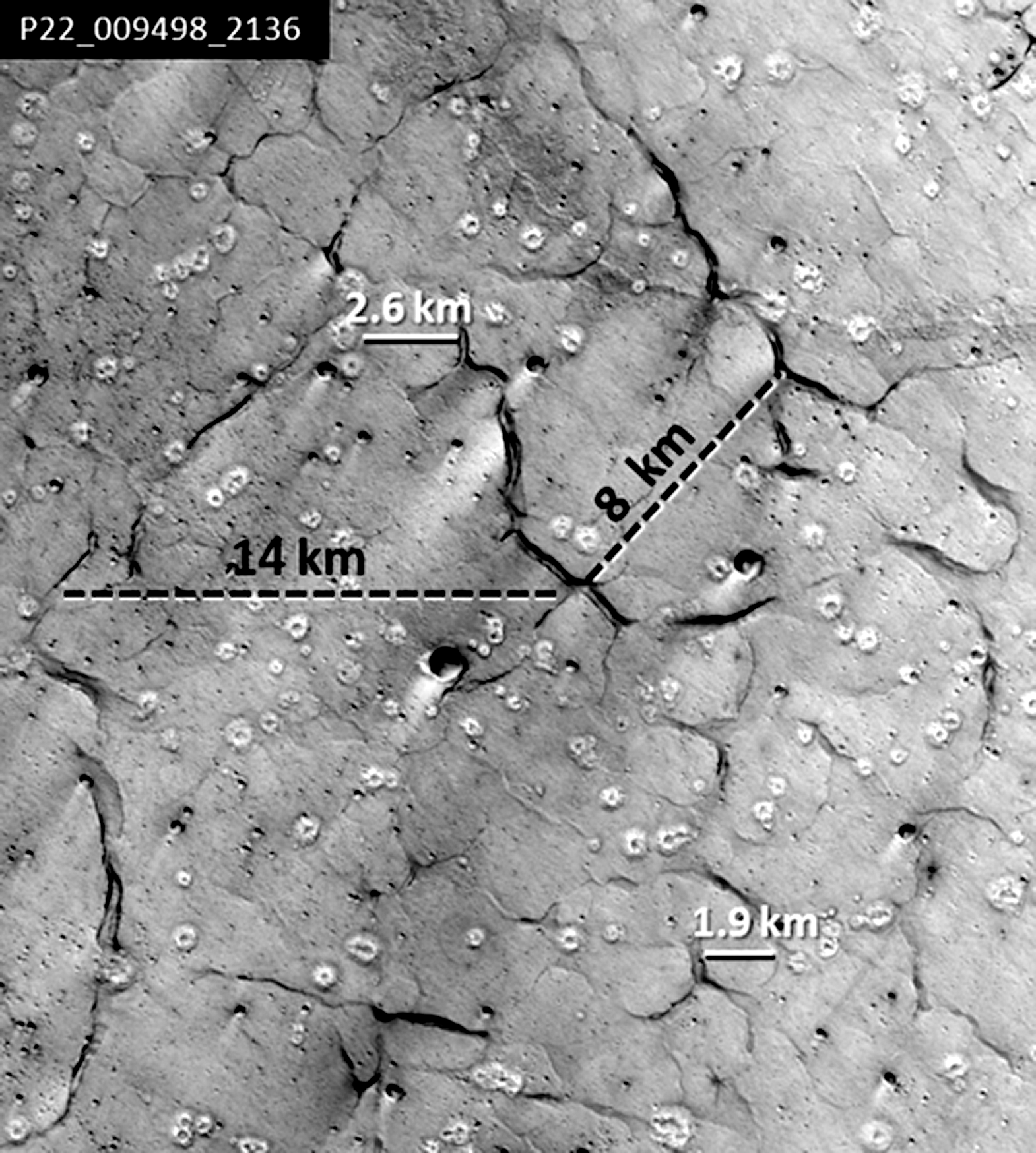
CTX image of giant polygons and mounds in a large ghost crater in northern Chryse Planitia. Black dashed scales indicate approximate sizes of first-order polygons formed by larger, exposed polygonal fractures. White scales illustrate sizes of many of the second-order giant polygons in this image. Bright circular mounds (∼0.3 to 1 km in diameter) are abundant within this ghost crater. Centerpoint: 34.2°N, 323.3°E; location shown on Fig. 1.

FIG. 4.

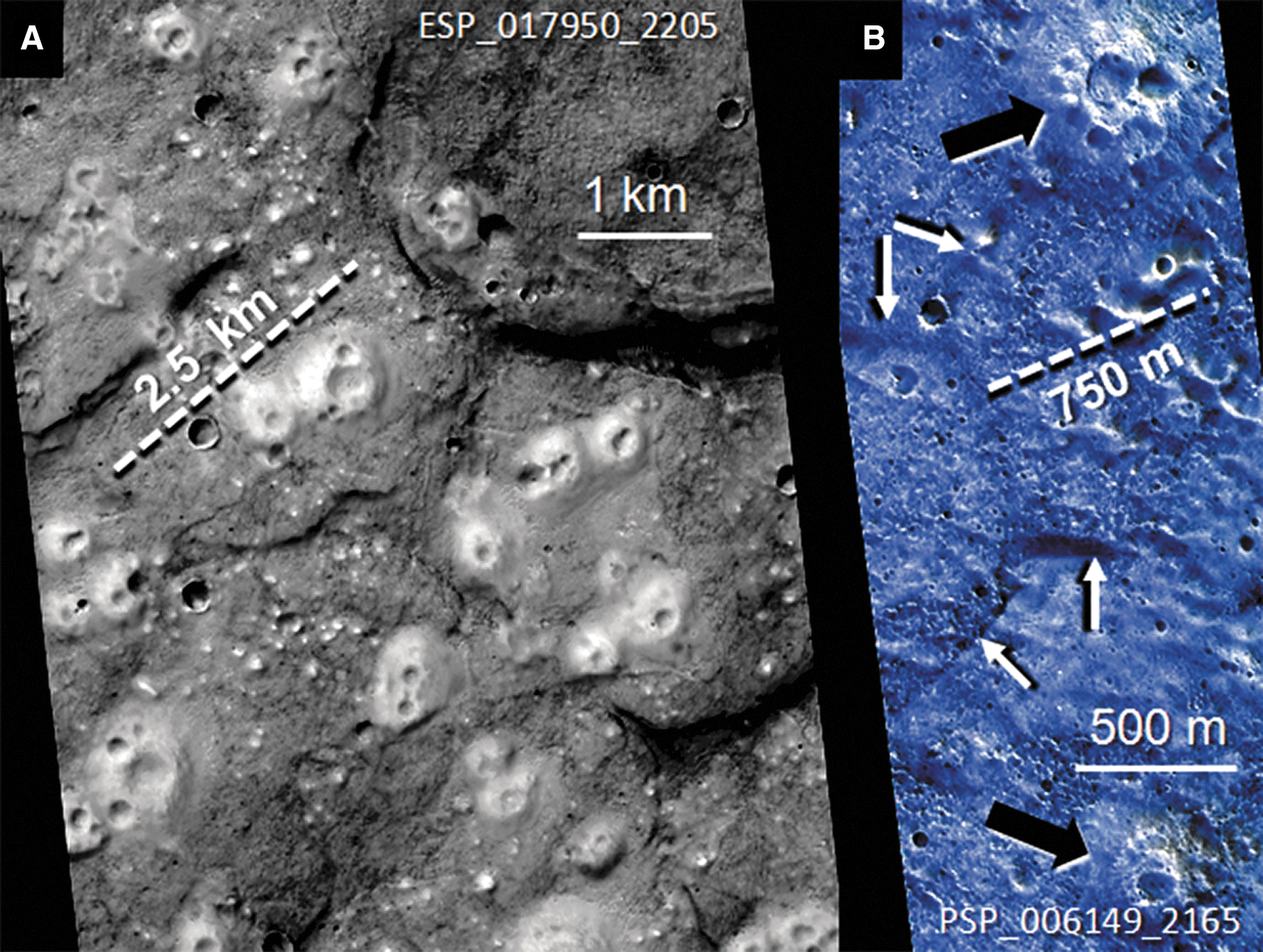
Detailed views of mounds and polygons in Acidalia from HiRISE images. (A) shows detail of ∼2.5 km second-order giant polygons and abundant mounds. (B) shows subtle polygons (thin white arrows) associated with bright mounds (thick black arrows). These subtle polygons were not observed in lower-resolution data sets. Centerpoint of (A): 40°N, 333.3°E. Centerpoint of (B): 36.3°N, 327.8°E. Locations of (A) and (B) shown on Fig. 1 Color image for panel B available online at www.liebertonline.com/ast.

Numerous investigators have addressed the origin of the giant polygons, with suggestions for their derivation including (i) extensional fracturing due to uplift resulting from unloading of water or ice (Pechmann, 1980; Hiesinger and Head, 2000a, 2000b); (ii) compaction of fluid-rich sediments over buried topography (Lucchitta et al., 1986; McGill, 1986; McGill and Hills, 1992; Buczkowski and Cooke, 2004); and (iii) a variant of the compaction/buried topography model involving catastrophic emplacement of water-saturated sediments on topographically irregular features followed by fluid convection of interstitial water within emplaced sediments (due to cooling at the sediment-atmosphere boundary); that convection is proposed to lead to differential thawing of underlying permafrost with subsequent compaction, thermal contraction, and desiccation (Lane and Christensen, 2000).

3.2. Mounds

More than 18,000 mounds have been mapped in a large area (2.5×10⁶ km²) of northern Chryse and southern Acidalia, and more than 40,000 are estimated to occur in that region (Amador et al., 2010; Oehler and Allen, 2010a). These mounds are typically bright circular features that are 0.3–2 km in diameter (Figs. 2B and 4) and variously pitted. Many have peripheral moats and central vents, and shape varies from splotches with low relief to domes and cones with several tens of meters of relief. Several of these mounds are associated with lobate extensions that resemble flows.

The origin of the mounds has been a subject of considerable discussion. They have been interpreted as pseudocraters (Frey and Jarosewich, 1982; Carr, 1986), cinder cones (Scott et al., 1995), pingos or ice-cored ridges (Lucchitta, 1981; Rossbacher and Judson, 1981), features related to moraines (Lucchitta, 1981; Scott and Underwood, 1990; Kargel and Strom, 1992; Lockwood et al., 1992), and ice disintegration features (Grizzaffi and Schultz, 1989). Recently, they have been interpreted as sedimentary diapirs, similar to terrestrial mud volcanoes (Tanaka 1997; Tanaka et al., 2003, 2005; Rodríguez et al., 2007; Skinner and Tanaka, 2007; Burr et al., 2009; McGowan, 2009; McGowan and McGill, 2009; Skinner and Mazzini, 2009; Oehler and Allen, 2010a) or to mud volcanoes combined with evaporite deposition around geysers or springs (Farrand et al., 2005).

3.3. Relationship between giant polygons and mounds in Chryse and Acidalia Planitiae

Most mounds in Chryse and Acidalia Planitiae occur in regions with extensively developed giant polygons, and both sets of features generally occur within the Vastitas Borealis Formation (VBF) (Fig. 5). This formation was considered by Kreslavsky and Head (2002) to be a sedimentary deposit formed from the Late Hesperian outflow sediments or their periglacially modified residues. Tanaka et al. (2005) noted that the VBF embays the Chryse channel system and thus might additionally include periglacially reworked plains deposits, spring discharges, or both; they mapped the VBF as Early Amazonian, but newer work suggests that the VBF will return to an older, end-of-Hesperian age (Tanaka, personal communication, 2012).

FIG. 5.

Comparison of mound and polygon occurrence with the Vastitas Borealis Formation (VBF) and elevation. MOLA shaded relief base map (polar projection). Thick red outline encloses generalized area within which 18,000+ mounds have been mapped, based on THEMIS Nighttime IR data (Oehler and Allen, 2010a). Elevation contours from MOLA data are overlain to illustrate relationship among the VBF, the mounds, and elevation. The southern and western boundaries of the red outline generally follow the elevation contours. The northern limit does not follow elevation, as that boundary reflects the limit of data with sufficient quality for mapping the mounds, so its deviation from elevation is not significant.

Figure 5 illustrates the correlation of the mounds and mapped giant polygons with the VBF and with elevation. Mapped mounds occur within the area enclosed by the red outline in Fig. 5 (Oehler and Allen, 2010a). The extent of the giant polygons is taken from mapping by Scott and Tanaka (1986) based on Viking data. Lucchitta et al. (1986) also mapped the giant polygons in this area from Viking data. While the Lucchitta et al. map shows a similar distribution of polygons in southern Acidalia, it includes an area of giant polygons north of 60°N within the Acidalia basin. The occurrence of mounds in that northern area was not assessed by Oehler and Allen (2010a), as the THEMIS Nighttime IR data set used to map the mounds was too poor in quality in that region to determine where mounds might be present. Accordingly, the northern boundary of the red outline on Fig. 5 simply marks the limit of good data. In the portion of southern Acidalia where mounds could be mapped, the areas with the highest mound spatial density commonly correlate with regions where giant polygons are muted and subdivided into second-order polygons (e.g., Fig. 2). Superposition relationships show that most mounds post-date the polygons, although the processes that formed each set of features may have overlapped in time (Oehler and Allen, 2010a). Both the mounds and giant polygons appear to be restricted to regions where accumulation of fine-grained, distal-facies sediments would be expected (Oehler and Allen, 2010b, 2012b; Allen et al., unpublished data).

From Fig. 5, it is also clear that the polygons and mounds generally occur within the Interior Unit of the VBF. A few occurrences of both mounds and polygons have been observed additionally in isolated patches of the Marginal Unit of the VBF. The distribution of the polygons, as indicated by both the Scott and Tanaka (1986) and Lucchitta et al. (1986) maps, is limited by the quality of the older Viking data, and new CTX and HiRISE images clearly show giant polygons beyond the areas mapped in those Viking-based studies (e.g., Figs. 3, 4, 6).

FIG. 6.

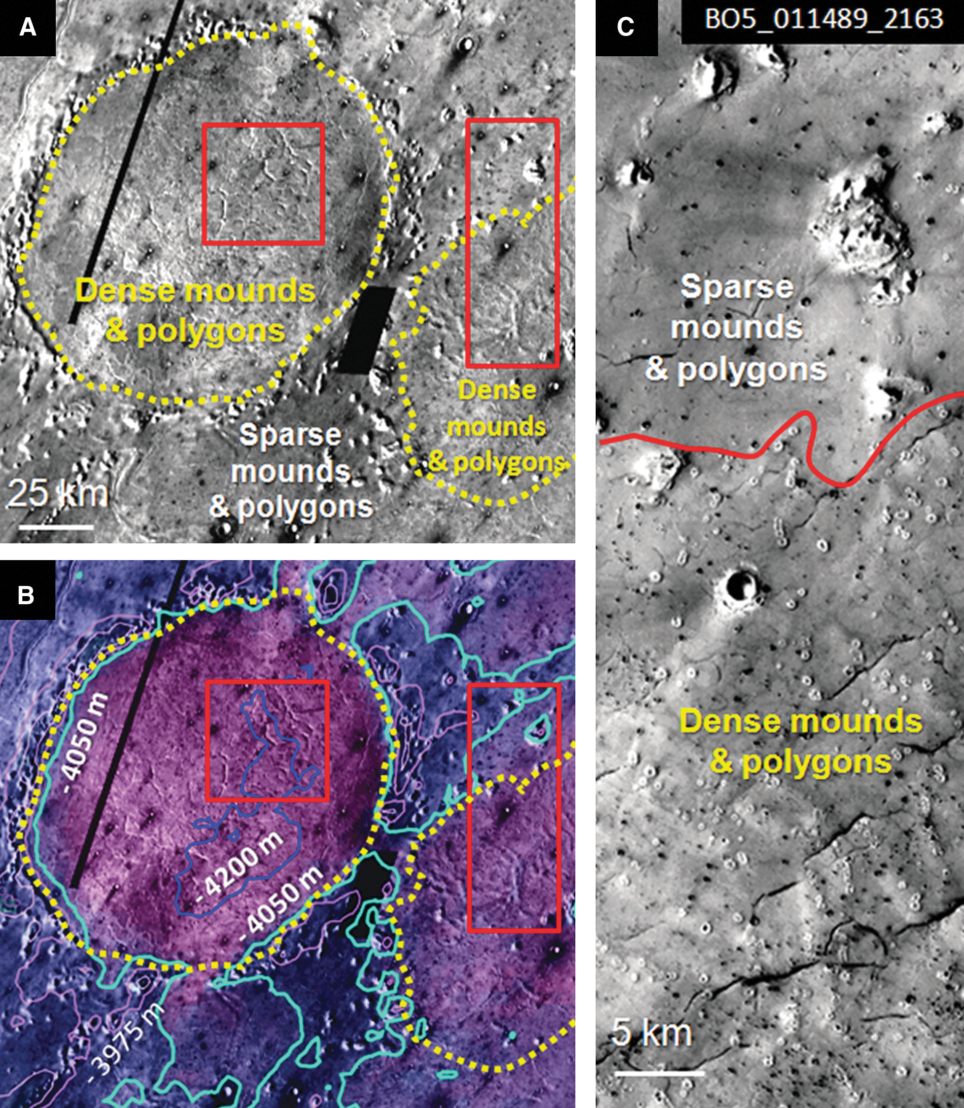
Images illustrating potential relationship of mounds and polygons to elevation. (A) THEMIS Daytime IR base map of northern Chryse (Mollweide projection), with the dotted yellow line marking a boundary between areas with dense mounds/polygons and those with sparse mounds/polygons. Red square on the left is the area of Fig. 3. Red rectangle on the right is the area of (C). (B) Same base map as (A), with overlays of elevation contours, elevation colors, and the mapped dotted yellow line boundaries separating areas with and without abundant mounds/polygons. Color scale is such that the pinker shade is deeper than the bluer shade. (C) CTX image of the area of the red rectangle on the right in (A), illustrating the quality of data possible with the 6 m/pixel CTX data set. Red line separates area of dense mounds and polygons to the south from area of sparse mounds and fewer polygons to the north. Centerpoint of (A) and (B): 33.8°N, 323.3°E; location shown on Fig. 1.

Work by McGowan (2009) on Cydonia Mensae (a small area within southern Acidalia) suggests that, in that particular area, the highest density of mounds occurs just south of, but separated from, the well-developed polygons. Nevertheless, some mounds do occur with the polygons, and conversely, there are suggestions of muted polygons in the area of dense mounds. The fact that the best-developed polygons coincide with a topographic low might suggest that erosion has played a role in exposing the polygons in that locality.

Acidalia Mensa, a high-standing platform within the Acidalia Basin, is surrounded by the mapped polygons (Fig. 5). The red outline of mound occurrence in Fig. 5 includes Acidalia Mensa, as there are numerous mounded features on that platform. However, data over Acidalia Mensa are still limited, and it is not certain that mounded structures on Acidalia Mensa were formed at the same time or by the same processes as mounds in the surrounding plains. Moreover, the red outline is a generalized depiction of the region in which the bright mounds have been observed, and it is anticipated that the new CTX data set will allow more detailed mapping of those features.

The VBF, the mounds, and the giant polygons exhibit potential relationships to present-day elevation (Fig. 5). The relationship between the polygons and elevation was noted by Head et al. (1999), who commented that the apparent relationship to elevation would be consistent with polygon formation in areas once occupied by a standing body of water. Regionally, the giant polygons and mounds are both most abundant below elevations of ∼−4000 m. One local area of northern Chryse has been studied in detail (Oehler and Allen, 2011, 2012a), and there the spatial density of the mounds increases dramatically below ∼−4050 m. The polygons in this area extend to slightly shallower elevations, being best developed below −3950 to −4000 m. However, neither polygons nor mounds occur above elevations of −3900 m (Fig. 6).

4. Terrestrial Fluid Expulsion Features

4.1. Large-scale polygons

Polygonal terrain is common in many settings on Earth. However, most terrestrial polygons are smaller than a few hundred meters across. The notable exceptions are the large-scale polygons, ∼ 0.5–3 km across, that develop in compacting marine mudstones (Fig. 7). These offshore polygonal fault systems went unrecognized for many years. But with the advent of 3-D seismic techniques in the 1990s, polygonal faults were discovered in the subsurface of numerous offshore basins, and in many cases these faults could be traced to shallow sediments, a few tens of meters below the sediment-water interface. Large-scale terrestrial polygons have since been studied in detail and are now recognized in more than 50 marine basins on Earth. In some of these basins, the polygons extend over regions greater than a million square kilometers (Cartwright, 1994, 1996; Cartwright and Lonergan, 1996; Cartwright and Dewhurst, 1998; Lonergan and Cartwright, 1999; Cartwright et al., 2003; Stuevold et al., 2003; Gay et al., 2004, 2006a).

FIG. 7.

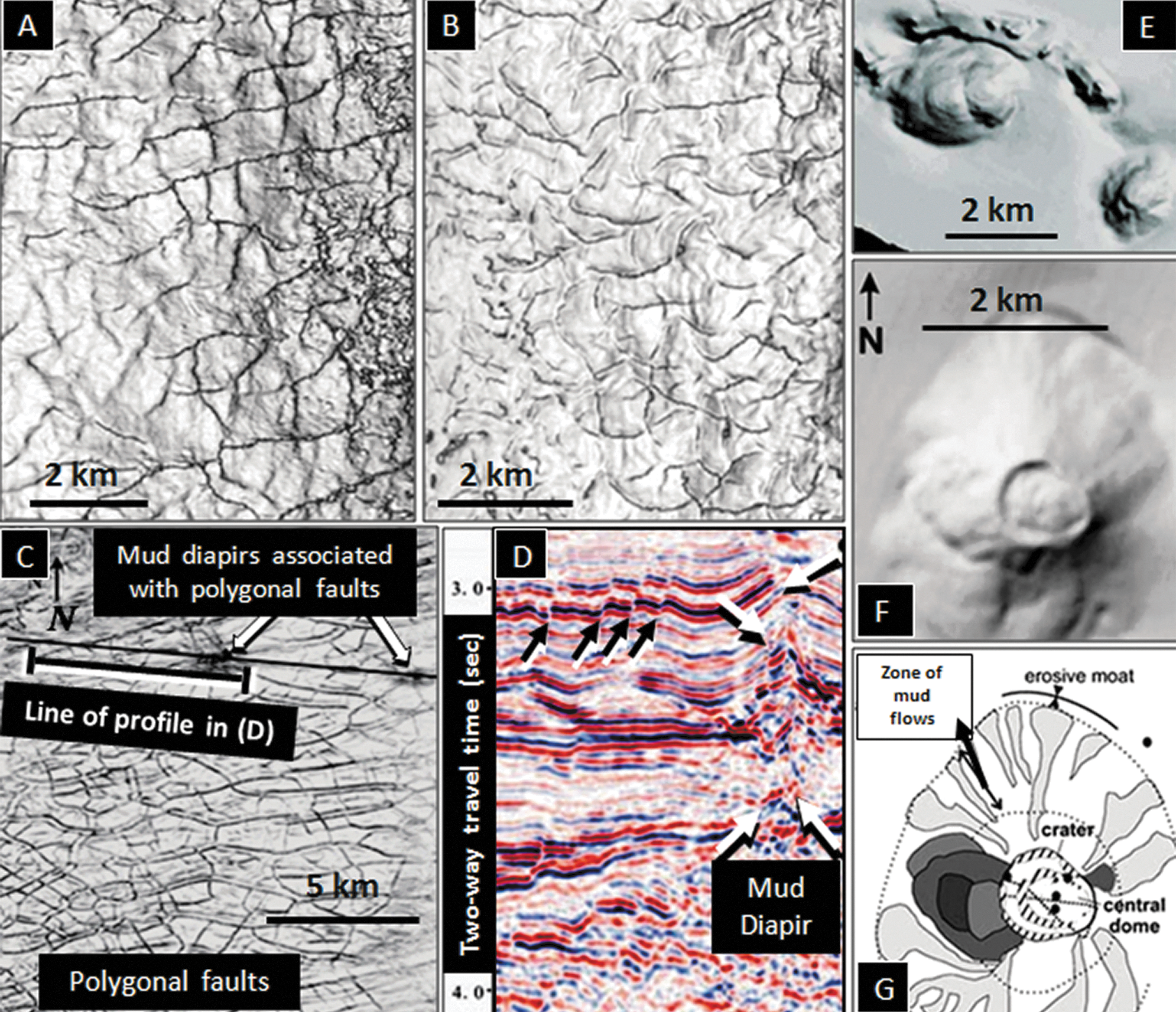
Terrestrial, offshore large-scale polygons and mud volcanoes. (A–C) Maps of large-scale terrestrial polygons from 3-D seismic data; (A, B) Offshore Norway (Stuevold et al., 2003); (C) South China Sea (Wang et al., 2010). (D) Seismic profile along trace shown in (C) illustrating polygonal faults (black arrows) and mud diapir (white arrows) (Wang et al., 2010). (E–F) Shaded relief from multibeam bathymetric sonar surveys of mud volcanoes in the El Arraiche mud volcano field, Gulf of Cadiz, offshore Morocco (Van Rensbergen et al., 2005a, 2005b); (E) Gemini, Don Quichote, and Fíuza mud volcanoes, (F) Al Idrissi mud volcano (the largest in the El Arraiche field, with a height of 255 m). (G) Interpretation map of Al Idrissi mud volcano showing individual mud flows (shaded and outlined areas), central crater and dome (striped pattern indicates slope areas in crater), overall zone of mud accumulation, and moat. Small black dots are locations that were sampled as part of the Van Rensbergen et al. (2005a, 2005b) survey. Color image of Fig. 7D available online at www.liebertonline.com/ast

Terrestrial large-scale polygons form in sediments at water depths of hundreds to thousands of meters and burial depths ranging from tens of meters to ∼1000 m. Their size range overlaps with the low end of the range typical of giant polygons in Acidalia (2–10 km) but is especially comparable to the size range of the second-order martian giant polygons (∼1–3 km) described above.

Large-scale terrestrial polygons are bordered by normal faults with modest offsets (10–100 m). Detailed map views constructed from time slices of 3-D seismic data show the shape, frequency, and stratigraphic associations of these polygons. In map view, morphologies range from hexagons to rectangles to shapes with curved boundaries (Fig. 7) (Cartwright et al., 2003). Vertically, these faults can extend from a few hundred meters to a kilometer. Fault frequencies and sizes of the polygons are related to a variety of parameters. For example, fault frequencies increase with burial depth (Gay et al., 2004) and with decreasing grain size (Dewhurst et al., 1999).

These large-scale terrestrial polygons are thought to be sediment compaction/dewatering features where the expelled fluids are released through the bounding faults and fractures. The polygons develop in thick, rapidly deposited sequences of mainly fine-grained sediments (claystones, shales) in settings that lack significant horizontal stress such as large offshore deltas and continental shelves on passive margins (Cartwright et al., 2003; Van Rensbergen et al., 2003, 2005a; Berndt, 2005; Gay et al., 2006a; Hustoft et al., 2007). These polygonal fault systems can be long-lived and provide sources of fluid into the shallow subsurface for millions of years (Berndt et al., 2003).

Various mechanisms have been put forth for the formation of terrestrial giant polygons, including gravity collapse, density inversion, syneresis, and compactional loading (Henriet et al., 1991; Cartwright and Dewhurst, 1998; Dewhurst et al., 1999; Goulty, 2001, 2008; Cartwright et al., 2003). At a minimum, 3-D contraction and dewatering due to loading are involved. Gay et al. (2004) summarized the typical sequence of events that leads to polygonal fault formation in basins with progressive loading. They noted that as sediment porosity decreases with compaction, so does permeability (due to particle reorientation and fluid expulsion that leads to decrease of void spaces between particles). Their analysis of polygonal fracture development in the Lower Congo Basin (offshore West Africa), using 3-D seismic data, illustrated the following relationship to loading: Polygonal faulting begins as linear furrows that develop near the sediment-water interface, apparently in response to mono-directional volume contraction. At ∼21 m below the seafloor, sediment contraction becomes radial, and a hexagonal pattern of furrows develops. With burial >21 m, permeability decreases to the point where sediment strength is sufficient for the formation and maintenance of faults, and the polygonal furrows develop into polygonal faults. By 78 m burial, fault offset is visible on seismic data, and by 300 m burial, sediment shrinkage causes maximum slip along the fault planes. Further pore fluid expulsion requires formation of more closely spaced polygonal faults, and large polygons become divided into smaller, second-order polygons with increasing depth. At 700 m below the seafloor, compaction by shrinkage is completed, and the fault frequency has reached its maximum. While most large-scale polygonal faults are subseafloor features, recent investigations of Hatton Bank (in the northeast Atlantic) provide an example of polygonal faults that reach the seafloor (Berndt et al., 2006).

Large-scale polygonal faults often are associated with offshore mud volcanoes and mud diapirs, and with gas seeps and the resultant depressions on the seafloor called pockmarks (Berndt et al., 2003; Van Rensbergen et al., 2003; Gay et al., 2004, 2006a, 2006b; Berndt, 2005; Gay and Berndt, 2007; Hustoft et al., 2007, Andresen et al., 2008; Chen et al., 2010; Huuse et al., 2010; Wang et al., 2010). Mud volcanoes and pockmarks represent end members of a variety of morphologies that can be produced by subsurface liquid and gas expulsion (Van Rensbergen, personal communication, 2012). In some settings, only one or two of these types of features occur, and the variability in fluid-expulsion expression is likely to be related to specifics of sediment character and setting (e.g., grain size, overburden, pore pressure, gas/liquid injection; Berndt et al., 2003). In this paper, we focus on associated mud volcanoes, as these are positive relief features to which the mounds in Acidalia have been recently compared (references noted in Section 3.2).

Figures 7C and 7D illustrate mud diapirs associated with polygonal terrain in the South China Sea. In this example, the polygons are relatively small. However, as noted above, marine polygonal faults increase in frequency with depth of burial, so that sizes of resultant polygons decrease with depth of burial. The polygonal faults in Fig. 7C are from a sediment package that is buried by more than 3 km of younger deposits, so the resulting map-view polygons may be at the small end of a typical size range because of that depth of burial.

4.2. Mud volcanoes

Mud volcanoes are mounded structures formed by erupting slurries of liquid, gas (usually methane), and mobilized sediment (Kopf, 2002; Deville et al., 2003, 2010; Van Rensbergen et al., 2003, 2005b; Deville, 2009; Huuse et al., 2010). Mud volcanoes have shapes that vary from relatively flat mounds to cones to domes. They can be as large as 10 km in diameter and several hundred meters in height. Mud volcanism is commonly related to overpressure that results from rapid deposition of fine-grained sediments, and episodes of mud volcanism can be triggered by events such as seismic disturbance, thermal pulses, and injection of gas from deep sources or shallow clathrate destabilization (Kopf, 2002; Mazurenko et al., 2002; Van Rensbergen et al., 2002).

Mud volcanoes generally occur in groups of tens to hundreds, although Deville (2009) estimated that tens of thousands may lie in the offshore. Mud volcanoes are well known in orogenic belts (such as those in Azerbaijan; Kopf, 2002) but recently have been found in offshore, passive-margin settings (e.g., deltas and continental shelves of the Congo River Basin, the Indus and Bengal Deltas, the Niger Delta, the Norwegian shelf, the South China Sea, and the Gulf of Mexico; Graue, 2000; Kopf, 2002; Van Rensbergen et al., 2002; Martinelli and Panahi, 2005; Stuevold et al., 2003; Gay et al., 2004, 2006a; Calvès et al., 2008, 2010; Deville, 2009; Etiope et al., 2009, 2011; Hustoft et al., 2010). Mud volcanoes can represent long-lived systems (with alternating active and dormant episodes spanning periods up to 20 million years; Calvès et al., 2010; Etiope et al., 2011), or they can represent shorter-lived systems, as suggested for the clathrate dissociation thought to be the cause of mud volcanism in Lake Baikal (Van Rensbergen et al., 2002).

5. Discussion

The relatively recent recognition of large-scale polygonal fault systems in offshore, marine basins on Earth is one of the unexpected results of 3-D seismic data acquisition. These fault systems seem potentially analogous to the giant polygons in the lowlands of Mars. The terrestrial polygons are similar in size to the martian second-order giant polygons now recognized in some of the higher-resolution orbital data sets. Terrestrial and martian polygons also share geological contexts. Terrestrial polygons form in areas of rapid accumulation of fine-grained sediment, in passive margins that lack significant horizontal stress. Martian giant polygons occur in a similar setting with regard to (i) predicted fine-grained facies (Oehler and Allen, 2012b); (ii) potentially rapid sediment accumulation from Hesperian outflow floods (Oehler and Allen, 2010a, 2012b); and (iii) lack of major horizontal stress, since Mars appears to have had minimal to no plate tectonics (Golombek, 2005; Golombek and Phillips, 2009), and contractional/extensional processes from the Noachian and Hesperian (Tanaka et al., 2005) may have been subsiding by the end Hesperian to Amazonian in the Chryse-Acidalia area.

At the same time, terrestrial mud volcanoes formed in passive margins may be analogous to the martian mounds, based on similar morphologies and common geological settings. In addition, the relatively low thermal inertia of the martian mounds suggests that, like mud volcanoes on Earth, the martian features may have brought uncompacted, fine-grained materials to the surface (Oehler and Allen, 2010a). The overlapping spatial distributions of giant polygons and mounds in Chryse and Acidalia Planitiae are similar to the association of large-scale, terrestrial polygons with various fluid expulsion features on Earth, and the basin-scale distributions of both sets of martian features strengthens the analogy to fluid expulsion features that extend across major marine basins on Earth.

The analogy requires that unconsolidated fine-grained sediments on Mars were compacted to form lithified sediments with sufficient strength to support fault development. On Earth, that typically occurs during burial. For Mars, previous work has suggested that late Hesperian floods debouched great quantities of sediment and water into Chryse and Acidalia through the outflow channels (Fig. 1) (Parker et al., 1993; Golombek et al., 1995a, 1995b; Rice and Edgett, 1997; Andrews-Hanna and Phillips, 2007; Andrews-Hanna and Lewis, 2011). The thickness of the sediments deposited by those floods is uncertain, and estimates range from 100 to 4500 m. McGill and Hills (1992) suggested a thickness of 600 m for polygon-forming terrain based on analyses of stealth craters. Zuber et al. (2000) estimated a thickness of 1000–4500 m based on topography, gravity, and inferred structure of the crust and upper mantle. Tanaka et al. (2001) estimated thicknesses of 1300–2800 m to account for a possible 900 m settling of Acidalia Mensa. And Kreslavsky and Head (2002) suggested a minimum, average thickness of ∼100 m based on analyses of stealth craters, roughness, and stratigraphic relationships. On Earth, polygonal faults start to form with loading >21 m (Gay et al., 2004). On Mars, compaction and lithification necessary to produce polygonal faulting might require more loading than on Earth because of Mars' lower gravity (∼38% of Earth's). However, the lowest thickness estimate for the outflow sediments (∼100 m) is a minimum average value (Kreslavsky and Head, 2002), and other estimates are considerably higher. Thus, it seems reasonable to speculate that loading from outflow sediments would have been sufficient to result in polygonal faulting in the Chryse-Acidalia part of the lowlands.

The Acidalia Mensa platform sits well within the Acidalia basin (Fig. 5), but its relationships to outflow sediments or an ancient ocean are uncertain. This platform is mainly comprised of the Marginal Unit of the VBF and the older Noachian, Noachis Terra Unit (Tanaka et al., 2005). Both units on the platform show major fractures and extensive evidence for fluidity (fluidized impact ejecta and bright lobate features). Bright mounds occur in both, and the Noachis Terra Unit includes numerous mounds associated with fractures and with troughs of potential polygons (Oehler and Allen, 2010a). The platform is embayed by the Interior Unit of the VBF. It is possible that Acidalia Mensa has been a high-standing body since the Noachian and that the fractures have provided avenues for upward fluid flow since that time. Similar situations are known from Earth, where buoyant basement blocks result in long-standing areas of indurated, high-standing materials that are surrounded by younger sedimentary accumulations (cf., the Cyrenaica Platform on the margin of the Sirte Basin of Libya; Benshati et al., 2009). If Acidalia Mensa were relatively high throughout much of martian history, then it may have acted as a partial barrier to northward deposition of sediments from the outflow events potentially enhancing accumulation of thick deposits of fine-grained materials immediately south of the platform.

On Earth, large-scale polygonal fractures and mud volcanoes only occur in sediments that were deposited in bodies of water. Even the many well-known examples of onshore mud volcanoes all involve mobilized sediments that were formed and buried in marine settings. If terrestrial large-scale polygons and mud volcanoes are reasonable analogues for the martian giant polygons and mounds, this analogy could imply that a large body of water—an ocean—existed at one time in northern Chryse and Acidalia. Accordingly, the distributions of the mounds and polygons there may map the extent of that body of water where the necessary conditions for polygon formation were met (e.g., fine-grained sediments, rapid burial, burial by at least tens of meters of sediment, and lack of overriding horizontal stress). It is also possible that an ancient ocean could have extended beyond the limits of the polygons and mounds in Chryse and Acidalia, into areas lacking either of these features. This could occur in regions where some conditions necessary for mound or polygon formation were not met and may account for portions of the lowlands where elevations are lower than −4000 m but where polygons appear not to occur.

The age of that body of water and the length of time it may have existed are remaining questions. Since the terrestrial polygons have been shown to form with a few tens of meters of burial, the presence of analogous features on Mars would not necessarily imply a geologically long-lived body of water. However, it has been suggested for Mars that standing bodies of water may have existed episodically in parts of the lowlands from the Noachian to the Amazonian (summarized by Dohm et al., 2008), ∼4.1 to less than ∼3.0 Ga (ages from Hartmann and Neukum, 2001). Since the giant polygons and mounds in Chryse and Acidalia are postdepositional features that occur mainly in the VBF (now thought to be of Late Hesperian age), these features would be Late Hesperian or younger and would postdate the Noachian to early Hesperian periods that are thought by many to have been the wetter times on Mars. Accordingly, areas with masses of giant polygons and mounds may record events in one of the later, major standing bodies of water.

The existence of a large body of water in northern Chryse–southern Acidalia would be consistent with data suggesting that this region had a fluid-rich history. These data include (i) evidence for Hesperian floods (Golombek et al., 1995a, 1995b; Rice and Edgett, 1997; Andrews-Hanna and Phillips, 2007); (ii) rampart craters with extensive fluidized ejecta (Barlow and Bradley, 1990; Barlow, 2001; Barlow and Perez, 2003; Martinez-Alonso et al., 2011); and (iii) hydrological models that suggest a high water table and concentration of upwelling ground waters in this region during the Noachian and Hesperian (Andrews-Hanna et al., 2007; Andrews-Hanna and Lewis, 2011).

More direct evidence may derive from the apparent correlation of martian giant polygons and mounds to elevation. Future mapping of the distributions of both polygons and mounds, with use of the CTX database (now providing nearly full coverage over much of the Chryse-Acidalia region) and HiRISE data where available, should provide a much more complete picture of the occurrences of these features, which can then be compared to elevation.

6. Conclusions and Implications

This paper presents the hypothesis that the genesis of mounds and giant polygons in the martian lowlands may be related to a common process—a process of fluid expulsion that involves burial and compaction of fine-grained sediments in an aqueous setting. We propose that the mounds and giant polygons in Chryse and Acidalia Planitiae are analogous to terrestrial mud volcanoes and kilometer-sized polygons that occur in passive-margin, marine shales. This interpretation is supported by the apparent correlation to elevation of the giant polygons and mounds in the Chryse-Acidalia area.

The hypothesis does not require that mounds and giant polygons are everywhere coincident or of identical ages, as it links the two sets of features to a progression of sedimentary events that would have varied in detail geographically. Rapid deposition of fine-grained sediments in an aqueous basin would be a necessary condition for the formation of mounds or polygons. But sufficient conditions for polygon formation may have varied from sufficient conditions for mound formation, and thus the two sets of features might be separated in time or space within the basin. Nevertheless, the widespread and generally overlapping occurrence of both mounds and polygons in the Chryse-Acidalia region suggests that the genesis of the two sets of features is linked and enhances the analogy to fluid expulsion features in marine settings on Earth.

The implications of this analogy are major. The distributions of the mounds and polygons in Chryse and Acidalia may map the minimum extent of a substantial body of water (>1 million square kilometers). Moreover, that body of water may have been one of the later repositories of liquid water on the planet, and as such, its location may be of importance in the search for long-lived habitable environments and evidence of past life on Mars.

Detailed mapping of the martian giant polygons and mounds, using the growing high-resolution orbital image coverage, should provide new data with which this hypothesis can be evaluated.

Footnotes

Acknowledgments

We are grateful to Dr. P. Van Rensbergen (Shell International Exploration and Technology, Rijswijk, The Netherlands) for discussions regarding the occurrence of giant polygons and mud volcanoes in offshore settings. We also are grateful to Drs. K.L. Tanaka, S.M. Clifford, and T.J. Parker for many helpful comments and suggestions. Support for this work was provided by the Astromaterials Research and Exploration Science (ARES) Directorate at Johnson Space Center (JSC) and by a grant from the Innovative Research and Development program at JSC. We thank the American Geophysical Union, the Geological Society of London, and John Wiley and Sons for granting permission to use portions of published images in of this paper.

Disclosure Statement

No competing financial interests exist.

Abbreviations

CTX, Context (camera); HiRISE, High Resolution Imaging Science Experiment; MOLA, Mars Orbiter Laser Altimeter; MRO, Mars Reconnaissance Orbiter; THEMIS, Thermal Emission Imaging System; VBF, Vastitas Borealis Formation.

References

Amador

E.S.

, Allen

C.C.

, Oehler

D.Z.

2010. Regional mapping and spectral analysis of mounds in Acidalia Planitia, Mars [abstract 1037] 41st Lunar and Planetary Science Conference. Lunar and Planetary Institute: Houston.

Andresen

K.J.

, Huuse

, Clausen

O.R.

2008. Morphology and distribution of Oligocene and Miocene pockmarks in the Danish North Sea—implications for bottom current activity and fluid migration. Basin Research, 20:445–466.

Andrews-Hanna

J.C.

, Lewis

K.W.

2011. Early Mars hydrology: 2. Hydrological evolution in the Noachian and Hesperian epochs. J Geophys Res, 116. doi:10.1029/2010JE003709.

Andrews-Hanna

J.C.

, Phillips

R.J.

2007. Hydrological modeling of outflow channels and chaos regions on Mars. J Geophys Res, 112. doi:10.1029/2006JE002881.

Andrews-Hanna

J.C.

, Phillips

R.J.

, Zuber

M.T.

2007. Meridiani Planum and the global hydrology of Mars. Nature, 446:163–166.

Baker

V.R.

, Strom

R.G.

, Gulick

V.C.

, Kargel

J.S.

, Komatsu

, Kale

V.S.

1991. Ancient oceans, ice sheets, and the hydrological cycle of Mars. Nature, 352:589–594.

Barlow

N.G.

2001. Impact craters as indicators of subsurface volatile reservoirs [abstract 7008] Conference on Geophysical Detection of Subsurface Water on Mars. Lunar and Planetary Institute: Houston.

Barlow

N.G.

, Bradley

T.L.

1990. Martian impact craters: dependence of ejecta and interior morphologies on diameter, latitude, and terrain. Icarus, 87:156–179.

Barlow

N.G.

, Perez

C.B.

2003. Martian impact crater ejecta morphologies as indicators of the distribution of subsurface volatiles. J Geophys Res, 108. 10.1029/2002JE002036.

10.

Benshati

, Khoja

, Sola

2009. Infracambrian sediments in Libyan sedimentary basins. Global Neoproterozoic Petroleum Systems: The Emerging Potential in North Africa

Craig

, Thurow

, Thusu

, Whitham

, Abutarruma

Geological Society. London: Special Publications. 326:181–191.

11.

Berndt

2005. Focused fluid flow in passive continental margins. Philos Transact A Math Phys Eng Sci, 363:2855–2871.

12.

Berndt

, Bünz

, Mienert

2003. Polygonal fault systems on the mid-Norwegian margin: a long-term source for fluid flow. Subsurface Sediment Mobilization. Van Rensbergen

, Hillis

R.R.

, Maltman

A.J.

, Morley

C.K.

Geological Society, London: Special Publications. 216:283–290.

13.

Berndt

, Jacobs

, Gay

, Hitchen

, Long

2006. Km-scale polygonal seafloor depressions in the Hatton Basin: new clues on the origin of polygonal fault systems. Geophysical Research Abstracts, 8SRef-ID: 1607-7962/gra/EGU06-A-05580European Geosciences Union, General Assembly: Vienna, Austria.

14.

Boyce

J.M.

, Mouginis-Mark

, Garbeil

2005. Ancient oceans in the northern lowlands of Mars: evidence from impact crater depth/diameter relationships. J Geophys Res, 110. doi:10.1029/2004JE002328.

15.

Buczkowski

D.L.

, Cooke

M.L.

2004. Formation of double-ring circular grabens due to volumetric compaction over buried impact craters: implications for thickness and nature of cover material in Utopia Planitia, Mars. J Geophys Res, 109. doi:10.1029/2003JE002144.

16.

Burr

D.M.

, Tanaka

K.L.

, Yoshikawa

2009. Pingos on Earth and Mars. Planet Space Sci, 57:541–555.

17.

Calvès

, Huuse

, Schwab

A.M.

2008. Three-dimensional seismic analysis of high-amplitude anomalies in the shallow subsurface of the Northern Indus Fan: sedimentary and/or fluid origin. J Geophys Res, 113. doi:10.1029/2008JB005666.

18.

Calvès

, Schwab

A.M.

, Huuse

, Van Rensbergen

, Clift

P.D.

, Tabrez

A.R.

, Inam

2010. Cenozoic mud volcano activity along the Indus Fan: offshore Pakistan. Basin Research, 22:398–413.

19.

Carr

M.H.

1986. Mars—a water-rich planet? Icarus, 68:187–216.

20.

Cartwright

J.A.

1994. Episodic basin-wide fluid expulsion from geopressured shale sequence in the North Sea Basin. Geology, 22:447–450.

21.

Cartwright

J.A.

1996. Polygonal fault systems: a new type of fault structure revealed by 3-D seismic data from the North Sea Basin. Applications of 3-D Seismic Data to Exploration and ProductionAAPG Studies in Geology 42 and SEG Geophysical Developments Series 5 Weimer

, Davis

T.L.

the American Association of Petroleum Geologists and the Society of Exploration Geophysics225–230.

22.

Cartwright

J.A.

, Dewhurst

D.N.

1998. Layer-bound compaction faults in fine-grained sediments. Geol Soc Am Bull, 110:1242–1257.

23.

Cartwright

J.A.

, Lonergan

. 1996. Volumetric contraction during the compaction of mudrocks: a mechanism for the development of regional-scale polygonal fault systems. Basin Research, 8:183–193.

24.

Cartwright

, James

, Bolton

2003. The genesis of polygonal fault systems: a review. Subsurface Sediment Mobilization. Van Rensbergen

, Hillis

R.R.

, Maltman

A.J.

, Morley

C.K.

Geological Society, London: Special Publications. 216:223–243.

25.

Chen

S.-C.

, Hsu

S.-K.

, Tsai

C.-H.

, Ku

C.-Y.

, Yeh

Y.-C.

, Wang

2010. Gas seepage, pockmarks and mud volcanoes in the near shore of SW Taiwan. Marine Geophysical Research, 31:133–147.

26.

Clifford

S.M.

, Parker

T.J.

2001. The evolution of the martian hydrosphere: implications for the fate of a primordial ocean and the current state of the Northern Plains. Icarus, 154:40–79.

27.

Deville

2009. Mud volcano systems. Volcanoes: Formation, Eruptions and Modelling. Lewis

, Moretti

Nova Science Publishers: Hauppauge, NY, 95–125.

28.

Deville

, Battani

, Griboulard

, Guerlais

, Herbin

J.P.

, Houzay

J.P.

, Muller

, Prinzhofer

2003. The origin and process of mud volcanism: new insights from Trinidad. Subsurface Sediment Mobilization. Van Rensbergen

, Hillis

R.R.

, Maltman

A.J.

, Morley

C.K.

Geological Society, London: Special Publications. 216:475–490.

29.

Deville

, Guerlais

S.-H.

, Lallemant

, Schneider

2010. Fluid dynamics and subsurface sediment mobilizatioin processes: an overview from Southeast Caribbean. Basin Research, 22:361–379.

30.

Dewhurst

D.N.

, Cartwright

, Lonergan

1999. The development of polygonal fault systems by syneresis of colloidal sediments. Marine and Petroleum Geology, 16:793–810.

31.

Di Achille

, Hynek

B.M.

2010. Ancient ocean on Mars supported by global distribution of deltas and valleys. Nat Geosci, 3:459–463.

32.

Dohm

J.M.

, Baker

V.R.

, Boynton

W.V.

, Fairén

A.G.

, Ferris

J.C.

, Finch

, Furfaro

, Hare

T.M.

, Janes

D.M.

, Kargel

J.S.

, Karunatillake

, Keller

, Kerry

, Kim

K.J.

, Komatsu

, Mahaney

W.C.

, Schulze-Makuch

, Marinangeli

, Ori

G.G.

, Ruiz

, Wheelock

S.J.

2008. GRS evidence and the possibility of paleooceans on Mars. Planet Space Sci, 57:664–684.

33.

Etiope

, Feyzullayev

, Baciu

C.L.

2009. Terrestrial methane seeps and mud volcanoes: a global perspective of gas origin. Marine and Petroleum Geology, 26:333–344.

34.

Etiope

, Oehler

D.Z.

, Allen

C.C.

2011. Methane emissions from Earth's degassing: implications for Mars. Planet Space Sci, 59:182–195.

35.

Fairén

A.G.

, Dohm

J.M.

, Baker

V.R.

, de Pablo

M.A.

, Ruiz

, Ferris

J.C.

, Anderson

R.C.

2003. Episodic flood inundations of the northern plains of Mars. Icarus, 165:53–67.

36.

Farrand

W.H.

, Gaddis

L.R.

, Keszthlyi

2005. Pitted cones and domes on Mars: observations in Acidalia Planitia and Cydonia Mensae using MOC, THEMIS, and TES data. J Geophys Res, 110. doi:10.1029/2004JE002297.

37.

Frey

2008. Ages of very large impact basins on Mars: implications for the Late Heavy Bombardment in the inner Solar System. Geophys Res Lett, 35. doi:10.1029/2008GL033515.

38.

Frey

, Jarosewich

1982. Subkilometer martian volcanoes—properties and possible terrestrial analogs. J Geophys Res, 87:9867–9879.

39.

Frey

H.V.

2006. Impact constraints on, and a chronology for, major events in early Mars history. J Geophys Res, 111. doi:10.1029/2005JE002449.

40.

Gay

, Berndt

2007. Cessation/reactivation of polygonal faulting and effects on fluid flow in the Voring Basin, Norwegian Margin. Journal of the Geological Society, 164:129–141.

41.

Gay

, Lopez

, Cochonat

, Sermondadaz

2004. Polygonal faults-furrows system related to early stages of compaction—upper Miocene to recent sediments of the Lower Congo Basin. Basin Research, 16:101–116.

42.

Gay

, Lopez

, Cochonat

, Séranne

, Levaché

, Sermondadaz

2006a. Isolated seafloor pockmarks linked to BSR's, fluid chimneys, polygonal faults and stacked Oligocene-Miocene turbiditic palaeochannels in the Lower Congo Basin. Mar Geol, 226:25–40.

43.

Gay

, Lopez

, Cochonat

, Sermondadaz

, Séranne

2006b. Evidences of early to late fluid migration from an Upper Miocene turbiditic channel revealed by 3D seismic coupled to geochemical sampling within seafloor pockmarks, Lower Congo Basin. Marine and Petroleum Geology, 23:387–399.

44.

Ghatan

G.J.

, Zimbelman

J.R.

2006. Paucity of candidate coastal constructional landforms along proposed shorelines on Mars: implications for a northern lowlands-filling ocean. Icarus, 185:171–196.

45.

Golombek

M.P.

2005. Tectonics of Mars [paper No. 137-3, p 312] Geological Society of America Abstracts with Programs, 37. Geological Society of America: Boulder, CO.

46.

Golombek

M.P.

, Phillips

R.J.

2009. Mars tectonics. Planetary Tectonics. Watters

T.R.

, Schultz

R.A.

Cambridge University Press: Cambridge, 183–232.

47.

Golombek

M.P.

, Edgett

K.S.

, Rice

J.W.

Jr.

1995a. Mars Pathfinder Landing Site Workshop II: Characteristics of the Ares Vallis Region and Field Trips in the Channeled Scabland, WashingtonLPI Technical Report Number 95-01, Part 1Lunar and Planetary Institute: Houston.

48.

Golombek

M.P.

, Edgett

K.S.

, Rice

J.W.

Jr.

1995b. Mars Pathfinder Landing Site Workshop II: Characteristics of the Ares Vallis Region and Field Trips in the Channeled Scabland, WashingtonLPI Technical Report Number 95-01, Part 2Lunar and Planetary Institute: Houston.

49.

Goulty

N.R.

2001. Polygonal fault networks in fine-grained sediments—an alternative to the syneresis mechanism. First Break, 19:69–83.

50.

Goulty

N.R.

2008. Geomechanics of polygonal fault systems: a review. Petroleum Geoscience, 14:389–397.

51.

Graue

2000. Mud volcanoes in deepwater Nigeria. Marine and Petroleum Geology, 17:959–974.

52.

Greeley

, Guest

J.E.

1987. Geologic map of the eastern equatorial region of Mars. U.S. Geological Survey Miscellaneous Investigations SeriesMap I-1802-B, scale 1:15,000,000U.S. Geological Survey: Reston, VA.

53.

Grizzaffi

, Schultz

P.H.

1989. Isidis basin—site of ancient volatile-rich debris layer. Icarus, 77:358–381.

54.

Hartmann

W.K.

, Neukum

2001. Cratering chronology and the evolution of Mars. Space Sci Rev, 96:165–194.

55.

Head

J.W.

, Kreslavsky

M.A.

, Hiesinger

, Ivanov

M.A.

, Pratt

, Seibert

, Smith

D.E.

, Zuber

M.T.

1998. Oceans in the past history of Mars: test for their presence using Mars Orbiter Laser Altimeter (MOLA) data. Geophys Res Lett, 25:4401–4404.

56.

Head

J.W.

, Hiesinger

, Ivanov

M.A.

, Kreslavsky

M.A.

, Pratt

, Thomson

B.J.

1999. Possible ancient oceans on Mars: evidence from Mars Orbiter Laser Altimeter data. Science, 286:2137–2143.

57.

Henriet

J.P.

, De Batist

, Verschuren

1991. Early fracturing of Palaeogene clays, southernmost North Sea: relevance to mechanisms of primary hydrocarbon migration. Generation, Accumulation and Production of Europe's Hydrocarbons, Special Publication of the European Association of Petroleum Geoscientists, 1

Spencer

A.M.

Oxford University Press: New York, 217–227.

58.

Hiesinger

, Head

J.W.

2000a. Characteristics and origin of polygonal terrain in southern Utopia Planitia, Mars: results from Mars Orbiter Laser Altimeter and Mars Orbiter Camera data. J Geophys Res, 105. doi:10.1029/1999JE001193.

59.

Hiesinger

, Head

J.W.

2000b. Characterization and origin of giant polygons in Utopia Planitia, Mars: results from MOLA and MOC [abstract 1290] 31st Lunar and Planetary Science Conference. Lunar and Planetary Institute: Houston.

60.

Hustoft

, Meinert

, Bünz

, Nouzé

2007. High-resolution 3D-seismic data indicate focussed fluid migration pathways above polygonal fault systems of the mid-Norwegian margin. Mar Geol, 245:89–106.

61.

Hustoft

, Bünz

, Meinert

2010. Three-dimensional seismic analysis of the morphology and spatial distributuion of chimneys beneath the Nyegga pockmark field, offshore mid-Norway. Basin Research, 22:465–480.

62.

Huuse

, Jackson

C.A.-L.

, Van Rensbergen

, Davies

R.J.

, Flemings

P.B.

, Dixon

R.J.

2010. Subsurface sediment remobilization and fluid flow in sedimentary basins: an overview. Basin Research, 22:342–360.

63.

Kargel

J.S.

, Strom

R.G.

1992. Ancient glaciation on Mars. Geology, 20:3–7.

64.

Kopf

A.J.

2002. Significance of mud volcanism. Rev Geophys, 40:2–52.

65.

Kreslavsky

M.A.

, Head

J.W.

2002. Fate of outflow channel effluents in the northern lowlands of Mars: the Vastitas Borealis Formation as a sublimation residue from frozen ponded bodies of water. J Geophys Res, 107. doi:10.1029/2001JE001831.

66.

Lane

M.D.

, Christensen

P.R.

2000. Convection in a catastrophic flood deposit as the mechanism for the giant polygons on Mars. J Geophys Res, 105:17617–17627.

67.

Lockwood

J.F.

, Kargel

J.S.

, Strom

R.B.

1992. Thumbprint terrain on the northern plains: a glacial hypothesis [abstract 1395] 23rd Lunar and Planetary Science Conference. Lunar and Planetary Institute: Houston.

68.

Lonergan

, Cartwright

J.A.

1999. Polygonal faults and their influence on deep-water sandstone reservoir geometries, Alba Field. United Kingdom Central North Sea. AAPG Bulletin, 83:410–432.

69.

Lucchitta

B.K.

1981. Mars and Earth—comparison of cold-climate features. Icarus, 45:264–303.

70.

Lucchitta

B.K.

, Ferguson

H.M.

, Summers

1986. Sedimentary deposits in the northern lowland plains. J Geophys Res, 91,supplement E166 E174.

71.

Malin

M.C.

, Edgett

K.S.

1999. Oceans or seas in the martian northern lowlands: high resolution imaging tests of proposed coastlines. Geophys Res Lett, 26:3049–3052.

72.

Malin

M.C.

, Edgett

K.S.

2001. Mars global surveyor Mars orbiter camera: interplanetary cruise through primary mission. J Geophys Res, 106:23429–23570.

73.

Martinelli

Panahi

2005. Mud Volcanoes, Geodynamics and SeismicityNATO Science Series, IV. Earth and Environmental Sciences51:288. Springer: Dordrecht, The Netherlands.

74.

Martinez-Alonso

, Mellon

M.T.

, Banks

M.E.

, Keszthelyi

L.P.

, McEwen

A.S.

the HiRISE team. 2011. Evidence of volcanic and glacial activity in Chryse and Acidalia Planitiae, Mars. Icarus, 212:597–621.

75.

Mazurenko

L.L.

, Soloview

V.A.

, Belenkaya

, Ivanov

M.K.

, Pinheiro

L.M.

2002. Mud volcano gas hydrates in the Gulf of Cadiz. Terra Nova, 14:321–329.

76.

McEwen

A.S.

, Hansen

C.J

, Delamere

W.A.

, Eliason

E.M.

, Herkenhoff

K.E.

, Keszthelyi

, Gulick

V.C.

, Kirk

R.L.

, Mellon

M.T.

, Grant

J.A.

, Thomas

, Weitz

C.M.

, Squyres

S.W.

, Bridges

N.T.

, Murchie

S.L.

, Seelos

, Okubo

C.H.

, Milazzo

M.P.

, Tornabene

L.L.

, Jaeger

W.L.

, Byrne

, Russell

P.S.

, Griffes

J.L.

, Martínez-Alonso

, Davatzes

, Chuang

F.C.

, Thomson

B.J.

, Fishbaugh

K.E.

, Dundas

C.M.

, Kolb

K.J.

, Banks

M.E.

, Wray

J.J.

2007. A closer look at water-related geologic activity on Mars. Science, 317:1706–1709.

77.

McGill

G.E.

1986. The giant polygons of Utopia, northern martian plains. Geophys Res Lett, 13:705–708.

78.

McGill

G.E.

, Hills

L.S.

1992. Origin of giant martian polygons. J Geophys Res, 97:2633–2647.

79.

McGowan

2009. Spatial distribution of putative water related features in Southern Acidalia/Cydonia Mensae, Mars. Icarus, 202:78–89.

80.

McGowan

E.M.

2010. Significance of water-related features on MarsPh.D. thesisUniversity of Massachusetts Amherst: Amherst, Massachusetts.

81.

McGowan

E.M.

, McGill

G.E.

2009. Putative water-related features: Cydonia Mensae and Utopia Planitia, Mars [abstract 1295] 40th Lunar and Planetary Science Conference. Lunar and Planetary Institute: Houston.

82.

Oehler

D.Z.

, Allen

C.C.

2010a. Evidence for pervasive mud volcanism in Acidalia Planitia, Mars. Icarus, 208:636–657.

83.

Oehler

D.Z.

, Allen

C.C.

2010b. Sediment prediction through basin analysis: an example from Acidalia Planitia [abstract 6069] 1st International Conference on Mars Sedimentology and Stratigraphy. Lunar and Planetary Institute: Houston.

84.

Oehler

D.Z.

, Allen

C.C.

2011. Habitability of a large ghost crater in Chryse Planitia, Mars. Exploring Mars Habitability, June 13–15, 2011. Lisbon: Portugal.

85.

Oehler

D.Z.

, Allen

C.C.

2012a. Fluid expulsion, habitability, and the search for life on Mars [abstract 1044] 43rd Lunar and Planetary Science Conference. Lunar and Planetary Institute: Houston.

86.

Oehler

D.Z.

, Allen

C.C.

2012b. Focusing the search for biosignatures on Mars: Facies prediction with an example from Acidalia Planitia. Mars Sedimentology, SEPM Special Publication. Grotzinger

, Milliken

SEPM: Tulsa.

87.

Parker

T.J.

, Saunders

R.S.

, Schneegerger

D.M.

1989. Transitional morphology in west Deuteronilus Mensae, Mars: implications for modification of the lowland/upland boundary. Icarus, 82:111–135.

88.

Parker

T.J.

, Gorsline

D.S.

, Saunders

R.S.

, Pieri

D.C.

, Schneeberger

D.M.

1993. Coastal geomorphology of the martian northern plains. J Geophys Res, 98:11061–11078.

89.

Pechmann

J.C.

1980. The origin of polygonal troughs on the northern plains of Mars. Icarus, 42:185–210.

90.

Rice

J.W.

Jr. , Edgett

K.S.

1997. Catastrophic flood sediments in Chryse Basin, Mars, and Quincy Basin, Washington: application of sandar facies model. J Geophys Res, 102:4185–4200.

91.

Rodríguez

J.A.P.

, Tanaka

K.L.

, Kargel

J.S.

, Dohm

J.M.

, Kuzmin

, Fairén

A.G.

, Sasaki

, Komatsu

, Schulze-Makuch

, Jianguo

2007. Formation and disruption of aquifers in southwestern Chryse Planitia, Mars. Icarus, 191:545–567.

92.

Rossbacher

L.A.

, Judson

1981. Ground ice on Mars—inventory, distribution, and resulting landforms. Icarus, 45:39–59.

93.

Scott

D.H.

, Tanaka

K.L.

1986. Geologic map of the western equatorial region of Mars. U.S. Geological Survey Miscellaneous Investigations SeriesMap I-1802-A, scale 1:15,000,000U.S. Geological Survey: Reston, VA.

94.

Scott

D.H.

, Underwood

J.R.

Jr.

1990. Mottled terrain—a continuing martian enigma [abstract 1567] 21st Lunar and Planetary Science Conference. Lunar and Planetary Institute: Houston.

95.

Scott

D.H.

, Rice

J.W.

Jr. , Dohm

J.M.

1991. Martian paleolakes and waterways: exobiologic implications. Orig Life Evol Biosph, 21:189–198.

96.

Scott

D.H.

, Dohm

J.M.

, Rice

J.W.

Jr.

1995. Map of Mars showing channels and possible paleo lake basins. U.S. Geological Survey Miscellaneous Investigations SeriesMap I-2461, scale 1:30,000,000U.S. Geological Survey: Reston, VA.

97.

Skinner

J.A.

Jr. , Mazzini

2009. Martian mud volcanism: terrestrial analogs and implications for formational scenarios. Marine and Petroleum Geology, 26:1866–1878.

98.

Skinner

J.A.

Jr. , Tanaka

K.L.

2007. Evidence for and implications of sedimentary diapirism and mud volcanism in the southern Utopia highland-lowland boundary plain, Mars. Icarus, 186:41–59.

99.

Stuevold

L.M.

, Faerseth

R.B.

, Arnesen

, Cartwright

, Möller

2003. Polygonal faults in the Ormen Lange Field, More Basin, offshore Mid Norway. Subsurface Sediment Mobilization. Van Rensbergen

, Hillis

R.R.

, Maltman

A.J.

, Morley

C.K.

Geological Society, London: Special Publications. 216:263–281.

100.

Tanaka

K.L.

1997. Sedimentary history and mass flow structures of Chryse and Acidalia Planitiae, Mars. J Geophys Res, 102:4131–4150.

101.

Tanaka

K.L.

, Banerdt

, Kargel

J.S.

, Hoffman

2001. Huge, CO₂-charged debris-flow deposit and tectonic sagging in the northern plains of Mars. Geology, 29:427–430.

102.

Tanaka

K.L.

, Skinner

J.A.

Jr. , Hare

T.M.

, Joyal

, Wenker

2003. Resurfacing history of the northern plains of Mars based on geologic mapping of Mars Global Surveyor data. J Geophys Res, 108. doi:10.1029/2002JE001908.

103.

Tanaka

K.L.

, Skinner

J.A.

Jr. , Hare

T.M.

2005. Geologic Map of the northern plains of Mars. U.S. Geological Survey Scientific Investigations SeriesMap 2888U.S. Geological Survey: Reston, VA.

104.

Van Rensbergen

, De Batist

, Klerkx

, Hus

, Poort

, Vanneste

, Granin

, Khlystov

, Krinitsky

2002. Sublacustrine mud volcanoes and methane seeps caused by dissociation of gas hydrates in Lake Baikal. Geology, 30:631–634.

105.

Van Rensbergen

, Hillis

R.R.

, Maltman

A.J.

, Morley

C.K.

2003. Subsurface sediment mobilization: introduction. Subsurface Sediment Mobilization. Van Rensbergen

, Hillis

R.R.

, Maltman

A.J.

, Morley

C.K.

Geological Society, London: Special Publications. 216:1–8.

106.

Van Rensbergen

, Depreiter

, Pannemans

, Moerkerke

, Van Rooij

, Marsset

, Akhmanov

, Blinova

, Ivanov

, Rachidi

, Magalhaes

, Pinheiro

, Marinha Cunha

, Henriet

J.-P.

2005a. The El Arraiche mud volcano field at the Moroccan Atlantic slope, Gulf of Cadiz. Mar Geol, 219:1–17.

107.

Van Rensbergen

, Depreiter

, Pannemans

, Henriet

J.-P.

2005b. Seafloor expression of sediment extrusion and intrusion at the El Arraiche mud volcano field, Gulf of Cadiz. J Geophys Res, 110. doi:10.1029/2004JF000165.

108.

Wang

, Wu

, Yuan

, Wang

, Ma

, Yao

, Gong

, Zhang

2010. Geophysical signatures associated with fluid flow and gas hydrate occurrence in a tectonically quiescent sequence, Qiongdongnan Basin, South China Sea. Geofluids, 10:351–368.

109.

Zuber

M.T.

, Solomon

S.C.

, Phillips

R.J.

, Smith

D.E.

, Tyler

G.L.

, Aharonson

, Balmino

, Banerdt

W.B.

, Head

J.W.

, Johnson

C.L.

, Lemoine

F.G.

, McGovern

P.J.

, Neumann

G.A.

, Rowlands

D.D.

, Zhong

2000. Internal structure and early thermal evolution of Mars from Mars Global Surveyor topography and gravity. Science, 287:1788–1793.