Hospitable Archean Climates Simulated by a General Circulation Model

Abstract

Evidence from ancient sediments indicates that liquid water and primitive life were present during the Archean despite the faint young Sun. To date, studies of Archean climate typically utilize simplified one-dimensional models that ignore clouds and ice. Here, we use an atmospheric general circulation model coupled to a mixed-layer ocean model to simulate the climate circa 2.8 billion years ago when the Sun was 20% dimmer than it is today. Surface properties are assumed to be equal to those of the present day, while ocean heat transport varies as a function of sea ice extent. Present climate is duplicated with 0.06 bar of CO₂ or alternatively with 0.02 bar of CO₂ and 0.001 bar of CH₄. Hot Archean climates, as implied by some isotopic reconstructions of ancient marine cherts, are unattainable even in our warmest simulation having 0.2 bar of CO₂ and 0.001 bar of CH₄. However, cooler climates with significant polar ice, but still dominated by open ocean, can be maintained with modest greenhouse gas amounts, posing no contradiction with CO₂ constraints deduced from paleosols or with practical limitations on CH₄ due to the formation of optically thick organic hazes. Our results indicate that a weak version of the faint young Sun paradox, requiring only that some portion of the planet's surface maintain liquid water, may be resolved with moderate greenhouse gas inventories. Thus, hospitable late Archean climates are easily obtained in our climate model. Key Words: Early Earth—Atmosphere—Habitability. Astrobiology 13, 656–673.

1. Introduction

T he Sun was up to 25% less luminous during the Archean (Gough, 1981). However, despite the faint young Sun, geological evidence indicates that early Earth had liquid water in the near-surface environment, a paradox that has stubbornly resisted a self-consistent solution (Sagan and Mullen, 1972). Continuous evidence for ancient life beginning as early as 3.8 billion years ago (Ga) further supports the conclusion that the Archean was generally hospitable and had at least some temperate regions capable of supporting life (Mojzsis et al., 1996; Rosing, 1999; Tice and Lowe, 2004; Schopf, 2006; Allwood et al., 2006). Aside from evidence for widespread glaciation between 2.45 and 2.22 Ga (Evans et al., 1997) and a possible regional glaciation at 2.9 Ga (Young et al., 1998), direct evidence for glaciation is conspicuously absent from the rest of the Archean geological record. Taken along with evidence from the isotopic composition of ancient marine cherts (Knauth and Lowe, 2003; Robert and Chaussidon, 2006), researchers have generally concluded that early Earth must have been hot and devoid of ice (Kasting, 2010). However, the Archean geological record is both spatially and temporally sparse, and the paleolatitudes of samples are unknown (Feulner, 2012). Recent work suggests that by 2.8 Ga nearly 70% of the present-day volume of continental crust had been established; however, high crustal reworking rates imply that very little unaltered material from this time period remains left today for study (Dhuime et al., 2012). Thus, the absence of glacial deposits in Archean samples should not be considered as strong evidence for a completely ice-free planet particularly given meridional gradients of temperature experienced on Earth at present. Furthermore, the high seawater temperature interpretation of the isotopic composition of Archean cherts is not universally accepted (Kasting et al., 2006; Jaffrés et al., 2007; Shields and Kasting, 2007). A weaker version of the faint young Sun paradox may only require that liquid water was present on some part of the planet's surface.

A CO₂-rich atmosphere could easily have kept early Earth warm despite low solar luminosity (Kasting, 1987), but analysis of paleosols (Rye et al., 1995; Sheldon, 2006; Driese et al., 2011) and banded iron formations (Rosing et al., 2010) impose constraints on its paleoatmospheric concentration. Radiative-convective models (RCMs) infer that 0.03 bar of CO₂ is needed to compensate for a 20% reduction in the solar constant, marginally preventing runaway glaciation with global mean surface temperatures hovering at 273 K (Haqq-Misra et al., 2008; von Paris et al., 2008). However, a recent estimate based on the geochemical mass-balance of tonalite weathering profiles places paleoatmospheric CO₂ at the end of the Archean at no more than 50 times the present atmospheric level (PAL), ∼0.018 bar as an upper limit at 2.69 Ga (Driese et al., 2011). Estimates deduced from the presence of magnetite within banded iron formations suggest much tighter constraints on CO₂, limiting its paleoatmospheric concentration during the Archean to a mere ∼3 PAL (0.001 bar) (Rosing et al., 2010). However, this interpretation is controversial (Dauphas and Kasting, 2011; Reinhard and Planavsky, 2011). Additional greenhouse warming may be provided by methane. Photochemical-ecosystem models infer that up to 0.035 bar of CH₄ may have been maintained in the anoxic Archean atmosphere (Kharecha et al., 2005). However, a CH₄ greenhouse is self-limiting. Titan-like photochemical hazes can form with the ratio of CH₄:CO₂ as low as 0.1 (DeWitt et al., 2009). Thus, too much methane may result in the formation of optically thick organic hazes, which could have cooled early Earth, negating any gained greenhouse warming (Domagal-Goldman et al., 2008; Haqq-Misra et al., 2008). Nonetheless, using an RCM with interactive haze chemistry, Haqq-Misra et al. (2008) showed that suitable combinations of CO₂ and CH₄ can yield temperate solutions for the late Archean climate if one adopts the more lenient constraints on CO₂ posed by Driese et al. (2011) and Sheldon (2006) as opposed to the temperature-dependent constraints of Rye et al. (1995). Ammonia, carbonyl sulfide, and higher-order hydrocarbons have high greenhouse potentials and could aid in hotter climate solutions, but the stability of trace gas solutions is not unanimously corroborated by photochemical and climate calculations (Sagan and Mullen, 1972; Haqq-Misra et al., 2008; Ueno et al., 2009).

For the past two decades, paleoclimate modeling studies with relevance to the faint young Sun paradox have primarily used RCMs (Kasting et al., 1984; Kasting, 1987; Domagal-Goldman et al., 2008; Haqq-Misra et al., 2008; von Paris et al., 2008; Goldblatt et al., 2009b; Rosing et al., 2010; Wordsworth and Pierrehumbert, 2013). Only very limited research has been conducted to date on the Archean climate with the use of multidimensional models (Henderson-Sellers and Henderson-Sellers, 1988; Jenkins, 1993, 2001; Stone and Yao, 2004; Kienert et al., 2012). RCMs are attractive research tools because they are computationally fast and can incorporate self-consistent atmospheric chemistry appropriate for reduced atmospheres, a capability not yet included in three-dimensional models. However, RCMs have limitations when it comes to modeling climate. RCMs represent the entirety of planetary climate with a single globally averaged vertical column; thus they ignore latitudinally dependent processes.

Radiative convective models often omit clouds and fix the surface albedo to a singular and constant value. In RCM paleoclimate simulations, the standard procedure is to tune the surface albedo to duplicate modern climate under clear-sky conditions. The surface albedo is then held fixed in all subsequent simulations; thus the ice-albedo feedback and cloud feedbacks are ignored. The absence of realistic longwave cloud absorption in RCMs also leads to an overestimation of the radiative forcing from CO₂ by up to 25% when pCO₂=0.1 bar (Goldblatt and Zahnle, 2011). The difficulty in achieving hot Archean climates with RCMs and the stringent constraints on CO₂ posed by Rosing et al. (2010) have led to alternative theories for warming the Archean that invoke changes to the planetary albedo and meridional distribution of energy (Rossow et al., 1982; Henderson-Sellers and Henderson-Sellers, 1988; Jenkins, 1993, 2001; Rondanelli and Lindzen, 2010; Rosing et al., 2010). Here, the climate of the late Archean circa 2.8 Ga is studied using an atmospheric general circulation model coupled to a mixed-layer ocean model.

2. Methods

2.1. Overview

In the present study, we used a general circulation model (GCM) to study Archean climate. We used the Community Atmosphere Model version 3.0 (CAM3) from the National Center for Atmospheric Research (Collins et al., 2004). CAM3 is a widely used GCM and has been extensively validated against modern climate. Regional and seasonal biases are present, but global and annual mean climatological statistics agree well with modern climate (Collins et al., 2006; Hurrell et al., 2006). CAM3 consists of component atmosphere, ocean, land, and sea ice models. The model uses a finite-volume dynamical core (Lin and Rood, 1996). Simulations were conducted with 4°×5° horizontal resolution with 66 vertical levels extending up to 5×10⁻⁶ mb. This equates to a model top of ∼130 km in simulations of the present day and ∼90 km for Archean simulations. The difference in model top height stems from the lack of ozone in Archean simulations, which results in a cold upper atmosphere with compressed scale heights. Continental configurations, topography, planetary rotation rate, ocean heat transport, cloud droplet sizes, land-based glacial ice, and surface vegetation are assumed to be those of the present day. Thus here we isolate the effects of reduced solar insolation and increased greenhouse forcing. By following this methodology, we are making the implicit assumption that the atmosphere of the late Archean was “like” present-day Earth, an assumption also inherent in the surface albedo tuning procedure used in RCM paleoclimate studies (Kasting et al., 1984). While the late Archean surely had differing topography and surface features, appropriate boundary conditions for deep paleoclimates remain speculative at best (Rosing et al., 2010). Here, all simulations are initiated from present-day surface temperatures. Equilibrium climate is typically reached within ∼50 model years; however, to ensure that our results are robust against slow adjustment, simulations are run an additional 50–100 years after equilibration. For all simulations presented, equilibrium conditions with no noticeable systematic drift are reached for the quantities of global mean surface temperature, sea ice fraction, sea ice thickness, surface albedo, top-of-atmosphere (TOA) albedo, and snow areal coverage.

Archean simulations assume a solar constant of 1093.6 W m⁻², which is 80% of the present-day value. The mean sea level pressure is taken to be 1.013 bar. The composition of the Archean atmosphere is assumed to be 0.00933 bar of argon gas along with variable amounts of CO₂, CH₄, and N₂. Oxygen and ozone are removed. Partial pressures of CO₂ and CH₄ are varied, while partial pressure of N₂ is calculated as pN₂=1.013 - pCO₂ - pCH₄ - pAr in units of bars. Atmospheric CO₂ is varied up to a maximum of 0.2 bar, while CH₄ is taken to be either 0 or 0.001 bar. Note that, given our selections for mean sea level pressure, pCO₂, and pCH₄, pN₂ is equal to, or slightly greater than, its PAL in all simulations presented here. Estimates of the late Archean surface pressure from fossilized raindrop imprints suggest that it was probably not much different from today, though the authors leave open the possibility that pN₂ could have been as much as twice the PAL as an upper limit (Som et al., 2012).

2.2. Radiative transfer

A new radiative transfer model has been implemented into CAM3 that is specifically tuned for anoxic, high-CO₂, and high-CH₄ atmospheres. The model uses a two-stream radiative transfer solver with multiple scattering (Toon et al., 1989). Molecular absorption by H₂O, CO₂, and CH₄ gases is treated by using correlated k-distribution absorption coefficients that were calculated by the Atmosphere Environment Research Inc. line-by-line radiative transfer model (LBLRTM) with access to the HITRAN 2004 spectroscopic database (Mlawer et al., 1997; Clough et al., 2005; Rothman et al., 2005). Overlapping molecular absorption is handled by using an amount weighted scheme (Shi et al., 2009). Correlated k-distributions are calculated on 56 pressure levels ranging from 3.162 bar to 0.01 bar with successive pressure levels following log10(P ₁ /P ₂)=0.1. Eight equally spaced temperature levels are utilized from 80 to 360 K. A wide range in pressure and temperature space allows for accurate radiative transfer calculations for atmospheres vastly different from those of the present day, particularly with regard to the exceedingly cold stratospheric temperatures expected for an anoxic early Earth (von Paris et al., 2008). The longwave (10–2200 cm⁻¹) spectrum is divided into 13 spectral intervals, while the shortwave (2200–50000 cm⁻¹) spectrum is divided into 15 spectral intervals (Table 1). The division between longwave and shortwave spectral regions is chosen such that solar radiation is largely confined to the shortwave, while terrestrial radiation is largely confined to the longwave. Each spectral interval has eight Gauss points except for the three spectral intervals encompassing 500–820 cm⁻¹, which require 16 Gauss points to improve accuracy in the stratosphere. In this spectral region, CO₂ absorbs very strongly. Low atmospheric pressure in the upper atmosphere amplifies small errors in flux when calculating radiative heating rates, and thus extra spectral Gauss intervals are required. Continuum absorption for CO₂, N₂, H₂O self-broadening, and H₂O foreign broadening are fit to the MT_CKD continuum model, which is implemented as part of the LBLRTM (Clough et al., 2005). For low CO₂, continuum absorption is negligible; however, it becomes increasingly important as pCO₂ rises above 0.1 bar (Halevy et al., 2009). While uncertainties remain regarding the proper theoretical treatment of CO₂ continuum absorption, the MT_CKD parameterization provides a median solution among popular continuum absorption models in use today (Halevy et al., 2009). Rayleigh scattering is included with the parameterization of Vardavas and Carver (1984). CO₂ is more than twice as effective at Rayleigh scattering than is N₂; therefore, Rayleigh scattering becomes increasingly important in CO₂-rich atmospheres. Both ice and liquid cloud particles are treated with Mie scattering. The radiative effect of overlapping cloud layers is treated with the Monte Carlo Independent Column Approximation under the assumption of maximum-random overlap (Pincus et al., 2003; Barker et al., 2008). The solar spectrum is taken to have the identical relative strength with wavenumber as the present day and is evenly scaled down to a lower solar constant for Archean simulations.

Table 1.

Radiative Transfer Spectral Intervals and Absorbing Species

Interval	Wavenumber range (cm⁻¹)	Absorbing species	# Gauss points
1	10–350	H₂O	8
2	350–500	H₂O	8
3	500–630	H₂O, CO₂	16
4	630–700	H₂O, CO₂	16
5	700–820	H₂O, CO₂	16
6	820–980	H₂O, CO₂	8
7	980–1100	H₂O, CO₂	8
8	1100–1180	H₂O, CH₄	8
9	1180–1390	H₂O, CH₄	8
10	1390–1480	H₂O, CH₄	8
11	1480–1800	H₂O, CH₄	8
12	1800–2080	H₂O, CO₂	8
13	2080–2200	H₂O, CO₂	8
14	2200–2380	CO₂	8
15	2380–2600	CO₂	8
16	2600–3250	H₂O, CH₄	8
17	3250–4000	H₂O, CO₂	8
18	4000–4650	H₂O, CH₄	8
19	4650–5150	H₂O, CO₂	8
20	5150–6150	H₂O	8
21	6150–7700	H₂O, CO₂	8
22	7700–8050	H₂O	8
23	8050–12850	H₂O	8
24	12850–16000	H₂O	8
25	16000–22650	H₂O	8
26	22650–29000	none	8
27	29000–38000	none	8
28	38000–50000	none	8

The new radiative transfer code has been tested against the LBLRTM to ensure accuracy for expected Archean greenhouse gas inventories. Figure 1 shows the clear-sky downwelling longwave flux at the surface and the clear-sky net longwave flux at the tropopause (defined here as the 200 mb level) calculated for varying pCO₂ and pCH₄ applied to the US 1976 Standard Atmosphere profile but with ozone and oxygen removed. The net broadband flux at the tropopause is taken to be positive downward. The net flux at the tropopause gives a good indication of the correlation between surface temperature changes and varying greenhouse gas amounts, while the downwelling flux at the surface gives a better indication of the absolute accuracy of the radiative transfer scheme (Goldblatt et al., 2009a). Both surface and net flux calculations are accurate to within ∼1.5% of line-by-line results up through end-member cases of pCO₂=0.3 bar and pCH₄=0.01 bar. At present we do not treat non–local thermodynamic equilibrium processes; thus radiative heating and cooling rates are strictly valid only for atmospheric pressures greater than ∼0.05 bar (∼51 km in anoxic simulations, 65 km in present-day simulations) where local thermodynamic equilibrium conditions are met (Fomichev et al., 1998). Above this level, the assumption of local thermodynamic equilibrium begins to break down with decreasing pressure, and additional physics is needed to obtain accurate heating/cooling rate profiles. Note that, for simulations under the present-day solar constant, ozone and oxygen absorption coefficients are added to correlated k-distributions, requiring a remapping of spectral intervals presented in Table 1.

FIG. 1.

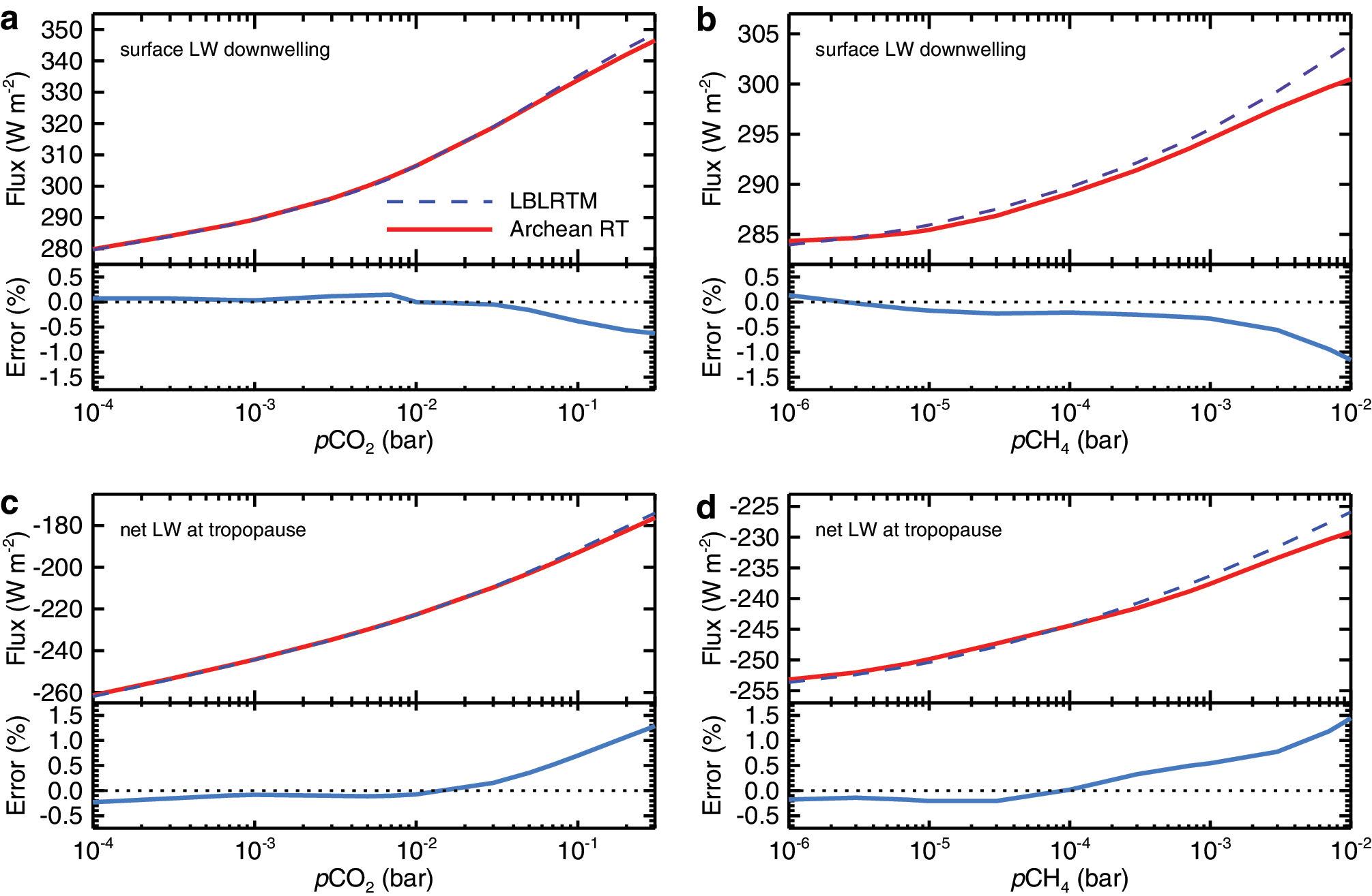
Longwave radiative fluxes from line-by-line calculations (LBLRTM, dashed blue) and from our model (Archean radiative transfer, red) assuming the US 1976 Standard Atmosphere but with oxygen and ozone removed. Panels (a) and (b) show the surface downwelling longwave flux and error compared with line-by-line calculations for varying CO₂ and CH₄, respectively. Panels (c) and (d) show the net longwave flux at the tropopause and error compared with line-by-line calculations for varying CO₂ and CH₄. Flux errors in our model remain less than ∼1.5% compared with line-by-line calculations. Color images available online at www.liebertonline.com/ast

2.3. Oceans and ice

CAM3 utilizes a mixed-layer ocean model coupled to a thermodynamic sea ice model (Collins et al., 2004, 2006). We chose to use a mixed-layer ocean model primarily due to the prohibitive computational expense of running a dynamic ocean model. Though the added computational overhead of coupling a dynamic ocean model to an atmospheric GCM is quite reasonable, spin-up times can be an order of magnitude longer than for GCMs run with a mixed-layer ocean model (Hansen et al., 2005). Here, our goal is to probe a wide range of atmospheric pCO₂, a task that would not be practical with a dynamic ocean model given our finite computational resources and time constraints. The thermodynamic sea ice model is based on the Community Sea Ice Model (Briegleb et al., 2004). The sea ice model calculates ice fractional coverage, ice thickness, surface temperature, snow depth, and an internal energy profile of the ice across four discrete layers. While the atmosphere adjusts quickly, the ocean–sea ice system can take several decades or more to reach thermal equilibrium. The contribution of snow to the total surface albedo can take up to ∼100 years to reach equilibrium (Mengel, 1988). Land glaciers are present at high latitudes and in mountainous regions with identical distributions as those of the present day. Land glaciers are treated as fixed surface features and do not respond to temperature.

Ice and snow albedo parameterizations include simple dependencies on wavelength and surface temperature. The wavelength dependency is split into visible (<0.7 μm) and near-IR (>0.7 μm) bands. For “cold” snow (sea ice) at surface temperatures below −1°C, the visible albedo is 0.96 (0.68), and the near-IR albedo is 0.68 (0.30). As the surface temperature rises from −1°C to the melting point (0°C), snow and sea ice albedos decrease following a linear temperature dependency to simulate the darkening of snow and sea ice surfaces during the melt process (Collins et al., 2004; Yang et al., 2012). For “warm” snow (sea ice) at surface temperatures of 0°C, the visible albedo is 0.86 (0.61), and the near-IR albedo is 0.53 (0.23). The albedo of land glaciers depends only on wavelength and is 0.80 in the visible and 0.55 in the near-IR. No melting is considered for land glaciers. The albedo of snow-covered surfaces is calculated as a weighted average between the snow-covered and bare surface fractions. Note that land glaciers and sea ice are often subject to persistent snow cover. The albedo of open ocean is 0.06 across all wavelengths.

The mixed-layer ocean model has seasonally and geographically varying depths between 10 and 200 m. A single temperature, characteristic of the entire mixed layer, is calculated via bulk energy balance equations between ocean, ice, and atmosphere at each ocean grid cell. While the mixed-layer ocean model is inherently motionless, deep ocean and horizontal transport is parameterized through the specification of a seasonally varying ocean internal heat flux convergence term (Q _flux). The initial set of Q _flux values is tuned to reproduce present-day ocean-to-atmosphere heat exchange and implicitly incorporate the effects of ocean circulations. As the planet cools, oceans tend to transport heat to the sea ice margin through convective mixing at the ice boundary and through wind-driven circulations (Poulsen et al., 2001). Qualitatively similar behavior is observed in our mixed-layer ocean model, which utilizes flux adjustments made to the initial set of Q _flux values as a function of changing sea ice cover (Fig. 2). The primary role of ocean heat transport is to remove heat from the tropics and deposit it at mid and high latitudes. Thus, the mean meridional structure of Q _flux is negative (divergence) in the tropics and positive (convergence) in the extra-tropics. Where Q _flux>0, heat is transferred from ocean to atmosphere. The locations with relatively stronger Q _flux convergence correlate to the leading edge of the sea ice as can be observed in Fig. 2. Thus, variations to the meridional structure of Q _flux, which in part is dictated by adjustments, can affect the location of the sea ice line, which in turn affects the global mean surface temperature. However, the stabilization of large polar cap climate states with sea ice extending into mid and low latitudes appears to be a robust feature of climate models, found in energy-balance models and GCMs utilizing both mixed-layer and dynamical ocean–sea ice models (Abbot et al., 2011; Ferreira et al., 2011; Voigt and Abbot, 2012; Yang and Peltier, 2012; Yang et al., 2012). Configured with a mixed-layer ocean model, CAM3 is suited to model climates centered on present-day surface temperatures that maintain large areas of open ocean. However, the simulation of a transition into a “snowball” climate state requires the use of dynamical ocean and sea ice models (Voigt and Abbot, 2012). See Section 3.2 for additional discussion of the model sensitivity to ocean and sea ice parameterizations.

FIG. 2.

Simulations are color-coded by mean surface temperature from warm (red, T _s=296.3) to cold (purple, T _s=230.2) and correspond with equilibrated climate simulations presented in Fig. 7. As sea ice expands (a), the ocean heat flux convergence (Q _flux) (b) is reduced in the tropics while increasing at mid and high latitudes. Positive values for Q _flux indicate a net transfer of heat from oceans to the atmosphere. Adjustments cause Q _flux to increase preferentially near the sea ice boundary, qualitatively similar to predictions made by dynamic ocean and sea ice models. Asymmetries in the zonal mean sea ice distribution are caused by the asymmetrical distribution of continents about the equator. Color images available online at www.liebertonline.com/ast

2.4. Clouds

Over the past two decades, cloud modeling has advanced tremendously such that realistic three-dimensional cloud fields can be considered in GCMs. Bulk microphysical parameterizations for condensation, precipitation, and evaporation control atmospheric water vapor, ice cloud condensate, and liquid cloud condensate fields (Rasch and Kristjánsson, 1998; Collins et al., 2004). Three types of clouds are treated. Marine stratus clouds depend on the stratification of the atmosphere between the surface and the 700 mb level (Klein and Hartmann, 1993). Convective clouds depend on the stability of the atmosphere and the upward convective mass flux (Xu and Krueger, 1991). Layered clouds at all altitudes depend on relative humidity and pressure. Liquid cloud droplet sizes are kept at their present-day values. Liquid cloud droplet effective radii vary from 8 to 14 μm over landmasses dependent on temperature, while effective radii are fixed at 14 μm over oceans and ice-covered regions. Ice particle effective radii follow a strictly temperature-dependent parameterization and can vary in size from a few tenths to a few hundred microns (Collins et al., 2004). Typical cirrus clouds in the model have ice particle effective radii of ∼50 μm at air temperatures of 240 K and ∼20 μm at air temperatures of 200 K.

3. Results

3.1. Standard atmospheres

Our simulations replicate modern climate with 360 ppm of CO₂, 1.7 ppm of CH₄, and a solar constant of 1367.0 W m⁻², yielding a global and annual mean surface temperature of 287.9 K and sea ice margin of 68.5°. Here, we calculate annual and global mean clear-sky radiative forcings. Radiative forcing is defined as the change in net downwelling radiative flux (F _down − F _up) at the tropopause caused by the introduction of a forcing agent (Hansen et al., 2005). The tropopause is defined as the lowest model level where the lapse rate (−dT/dZ) is 2 K/km or less (World Meteorological Organization, 1957). We define radiative forcings relative to our simulation of modern climate. Radiative forcing is a useful concept for estimating first-order changes to the planet's surface temperature caused by perturbations to the radiation field. However, the complex interaction of climate feedbacks with imposed radiative forcings ultimately determines the exact radiative forcing–surface temperature response.

We first performed a simulation using modern CO₂ and CH₄ concentrations after allowing the stratosphere to adjust to the removal of oxygen and ozone but with all other aspects of climate held fixed. Molecular nitrogen is increased to maintain the present-day mean sea level pressure of 1.013 bar (see Section 2.1). In this simulation, the global and annual mean surface temperature is 287.4 K, and the sea ice margin is 67.8° (see Table 2). Removing oxygen and ozone allows more solar radiation to reach the surface, yielding a small radiative forcing of +1.2 W m⁻². However, removing O₃ greatly reduces stratospheric temperatures and thus reduces downwelling longwave fluxes emanating from the upper atmosphere by ∼2 W m⁻². Combining the reduced radiation due to the stratospheric temperature change with the loss of ozone's greenhouse contribution, the removal of O₃ yields a longwave radiative forcing of −5.2 W m⁻².

Table 2.

Standard Atmospheres

Atmospheres	Present day	No ozone	Late Archean
Solar constant (W m⁻²)	1367.0	1367.0	1093.6
CO₂ (ppm)	360	360	60,000
CH₄ (ppm)	1.7	1.7	0
Mean Surface Temperature (K)	287.9	287.4	287.9
Tropical ocean mixed layer temperature (K)	291.1	290.7	290.3
Sea ice margin (degrees)	71.9	71.0	74.2
Latent heat flux (W m⁻²)	88.0	87.9	81.8
Sensible heat flux (W m⁻²)	21.1	20.6	18.6
Water column (kg m⁻²)
Water vapor	24.2	24.0	20.4
Cloud liquid water	0.116	0.115	0.086
Cloud ice water	0.0164	0.0171	0.0172
Cloud radiative forcings (W m⁻²)
Shortwave	−55.1	−55.5	−34.5
Longwave	30.2	34.1	25.4
Net	−24.9	−21.4	−9.1
Cloud fraction (%)
Low	39.2	38.7	31.0
Middle	22.3	22.2	23.3
High	36.0	49.4	53.9
Albedo
TOA	0.337	0.354	0.317
Surface	0.143	0.147	0.137
Cloud	0.168	0.168	0.135

Archean simulations assume a solar constant 80% of the present-day value. This equates to a clear-sky net downwelling radiative forcing of −56.7 W m⁻². In our model, we can achieve a global and annual mean surface temperature of 287.9 K, with 80% of the present-day solar constant assuming a CO₂ partial pressure of 0.06 bar (60,000 ppm), henceforth regarded as our “standard” Archean atmosphere (see Table 2). Increasing CO₂ from 360 ppm to 0.06 bar yields a longwave radiative forcing of +46.4 W m⁻². However, absorption of solar energy in the near-IR and enhanced Rayleigh scattering, both due to increased atmospheric CO₂, result in an additional shortwave radiative forcing of −2.7 W m⁻². The total change in global mean radiative forcing between our present-day and standard Archean simulations is calculated by summing the radiative forcings due to the removal of oxygen and ozone (+1.2 W m⁻² shortwave, −5.2 W m⁻² longwave), the reduction to the solar constant (−56.7 W m⁻² shortwave), and the increase in atmospheric CO₂ (−2.7 W m⁻² shortwave, +46.4 W m⁻² longwave). The remaining global mean energy deficit of −17.0 W m⁻² is accounted for through feedbacks involving the Archean hydrological cycle.

The Archean hydrological cycle is altered by fundamental changes to the radiative forcing at the surface caused by weak solar radiation and a strong greenhouse (Fig. 3a). The positive radiative forcing imposed by increasing the concentration of a well-mixed greenhouse species (in this case CO₂) has a weak latitudinal gradient compared with the negative forcing imposed by decreasing the solar constant, particularly across low latitudes. Weak radiant energy reaching the Archean surface inhibits the hydrological cycle by reducing surface latent heat fluxes (i.e., evaporation of water from ocean surfaces) over low latitudes compared with the present day despite mean tropical ocean temperatures that differ by less than 1 K (Fig. 3b). Zonal mean latent heat fluxes are reduced by on the order of 10 W m⁻² across the tropics. Reduced latent heat fluxes naturally result in reduced specific humidities in the lower troposphere of the Archean compared with the present day (Fig. 4b). Similar boundary-layer temperatures ensure that the Archean also has reduced relative humidities below ∼4 km (Fig. 4c). The reduction in moisture in the lower troposphere in turn leads to reductions in moist convective mass and water fluxes (Fig. 5) and reductions to low-level clouds (below 700 mb) (Fig. 6c). However, above the boundary layer the situation reverses. Our standard Archean atmosphere has slightly colder temperatures in the upper troposphere compared with the present day. Since the saturation vapor pressure depends exponentially on temperature, a small decrease in air temperature yields significant changes in relative humidity for a given amount of water vapor. Lower temperatures and larger relative humidities aloft imply a greater potential for latent heat release and thus reduced static stabilities. Thus, while shallow boundary-layer convection remains weak, deep convective mass and water fluxes are enhanced for the Archean (Fig. 5). Increased convection aloft helps support the higher-altitude cloud decks in the Archean despite an atmosphere with a reduced total water vapor column. Middle clouds (700–400 mb) are approximately equal to their present-day value, while high clouds (400 mb and upward) occur with an increased frequency (Fig. 6a, 6b).

FIG. 3.

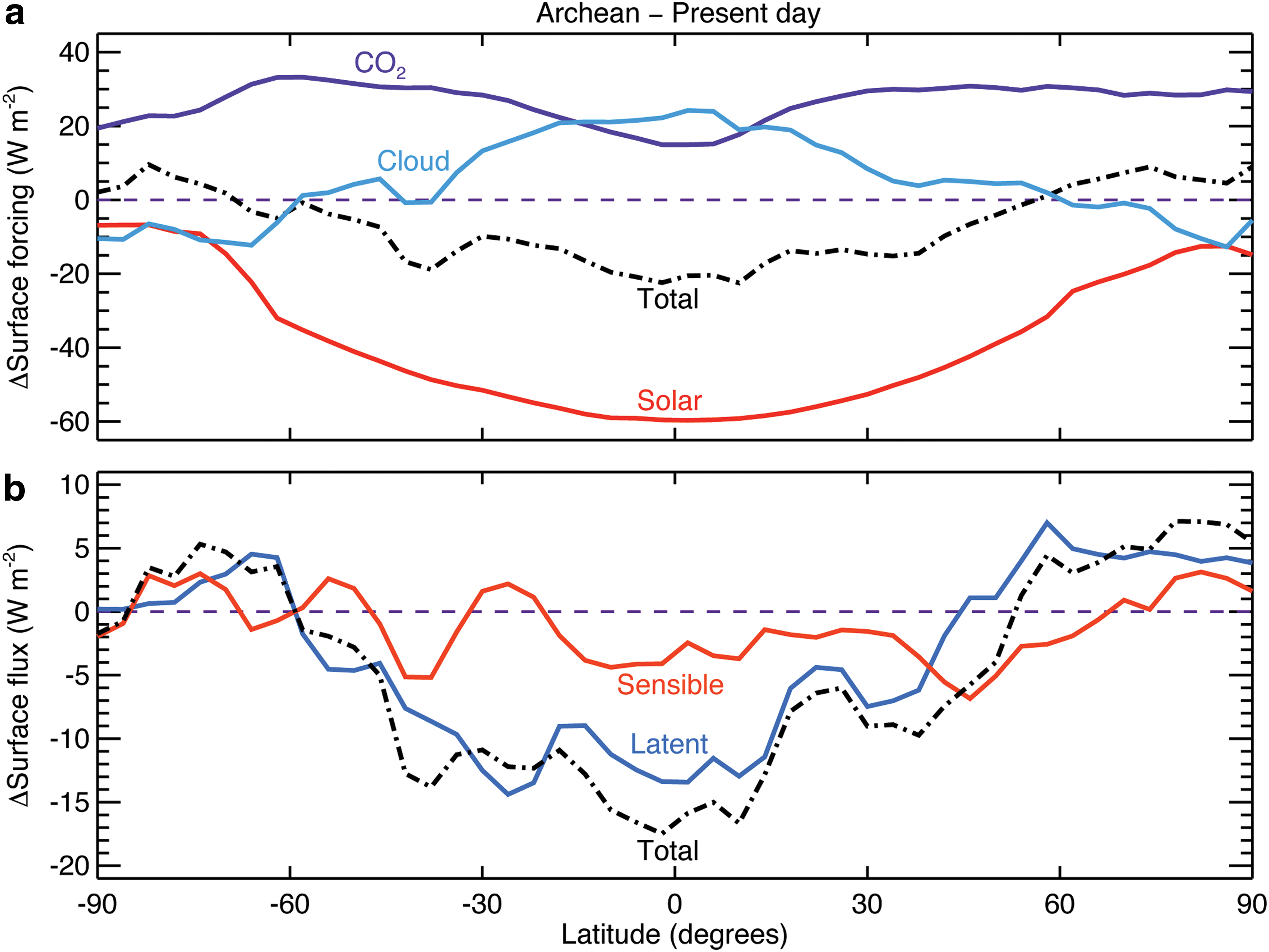
Zonal mean broadband surface forcing difference (a) and surface energy flux difference (b) between standard Archean and present-day atmospheres. A value of zero (dashed purple) means that the surface forcing for the late Archean and present-day atmospheres is identical. Positive values for surface forcing indicate relative warming, while negative values indicate relative cooling for the Archean compared to the present day. A large negative surface forcing caused by a 20% reduction in the solar constant (red) is offset by increased greenhouse forcing from 0.06 bar of CO₂ (dark blue). A weakening of the Archean hydrological cycle reduces water clouds and shortwave cloud forcing, allowing a greater fraction of the incident solar radiation to reach the tropical surface than at present (light blue). Despite identical mean surface temperatures, our standard Archean atmosphere receives more energy at the polar surface and less energy at the tropical surface compared with the present day (dash-dot black). Surface latent (blue) and sensible (red) heat fluxes are decreased compared with the present-day atmosphere coincident with reductions to the surface radiative forcing. Total (dash-dot black) surface fluxes are reduced by ∼17 W m⁻² at the equator; however, note that reductions to latent heat fluxes dominate. Color images available online at www.liebertonline.com/ast

FIG. 4.

Global and annual mean vertical profiles of temperature (a, d), specific humidity (b, e), and relative humidity (c, f) for Archean (red), present day (purple), and the present-day atmosphere but with oxygen and ozone removed (dashed light blue). The top panels show profiles for the troposphere, and the bottom panels show profiles for the whole atmosphere up to a height of 60 km. Color images available online at www.liebertonline.com/ast

FIG. 5.

(a) Tropical moist convective mass flux and (b) moist convective water flux for the Archean (red), present day (purple), and the present-day atmosphere but with oxygen and ozone removed (dashed light blue). Profiles are averaged between 22°S and 22°N latitudes. The reduction to surface latent heat flux inhibits shallow convection for our standard Archean atmosphere. However, a generally steeper lapse rate and higher relative humidities aloft allow convection to penetrate to higher altitudes. Color images available online at www.liebertonline.com/ast

FIG. 6.

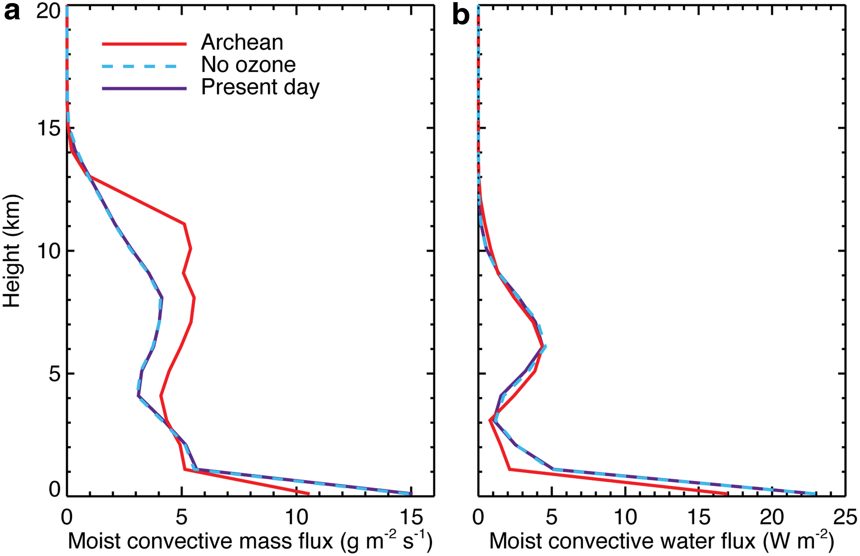
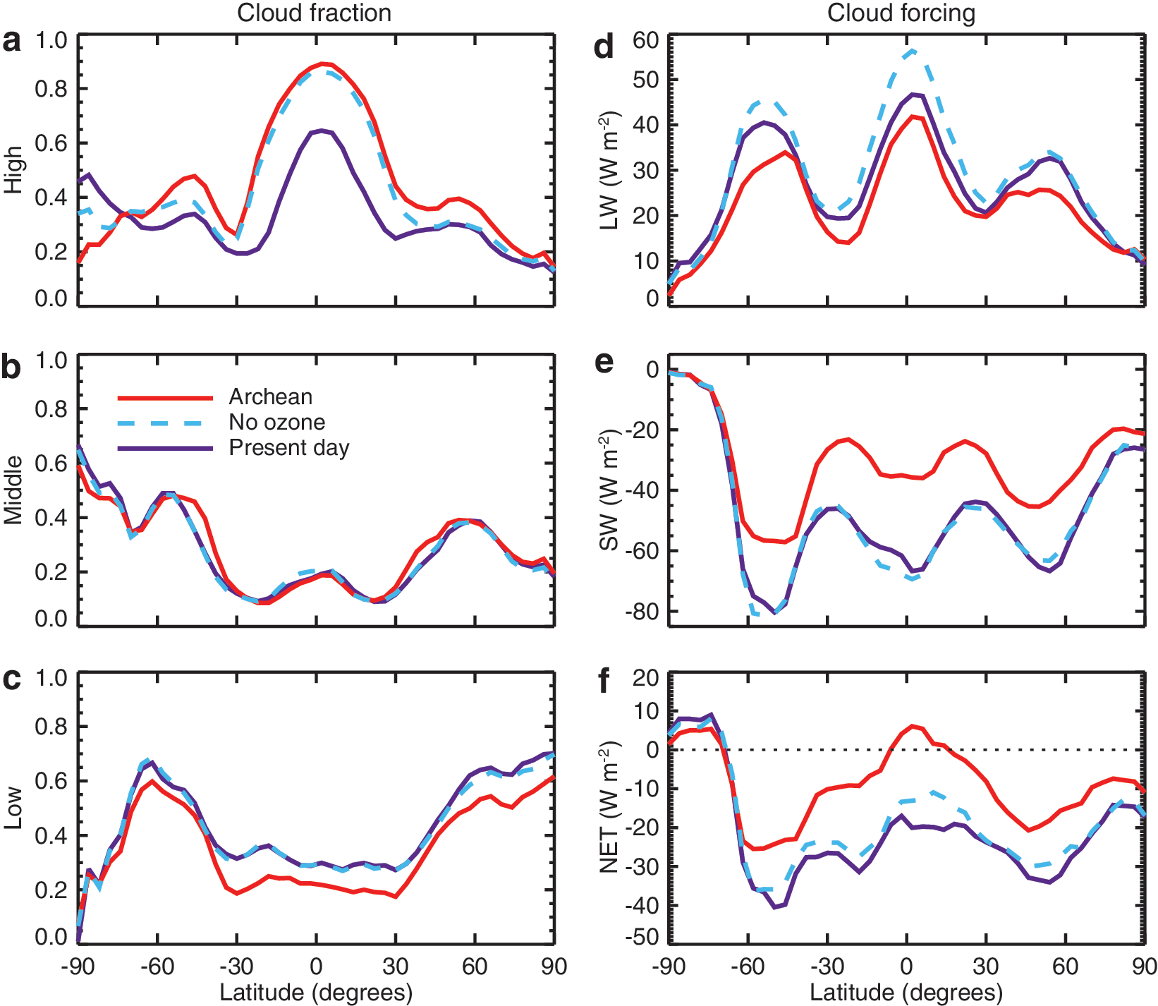
Zonal mean cloud properties for the Archean (red), present day (purple), and the present-day atmosphere but with oxygen and ozone removed (dashed light blue). (a) Vertically integrated high cloud fraction describes clouds above 400 mb (Z>6 km). (b) Vertically integrated middle cloud fraction describes clouds between 700 and 400 mb (2<Z<6 km). (c) Vertically integrated low cloud fraction describes clouds below 700 mb (Z<2 km). (d) Longwave cloud forcing, 10–2200 cm⁻¹. (e) Shortwave cloud forcing, 2200–50,000 cm⁻¹. (f) Net cloud forcing (longwave plus shortwave). Color images available online at www.liebertonline.com/ast

For our standard Archean atmosphere, the climatological mean atmospheric water vapor column is reduced by ∼16%, and the cloud water column is reduced by ∼26% compared with simulations of the present day. Global mean low cloud fractions and cloud albedos are reduced in nearly exact proportion with the reduction in the solar constant despite identical global mean surface temperatures, reinforcing the importance of solar energy for driving the hydrological cycle. While the water vapor greenhouse is weakened, reductions to low cloud fractions (Fig. 6c) greatly reduce the magnitude of the shortwave cloud forcing at the tropopause (Fig. 6e). The magnitude of the shortwave cloud forcing is reduced by 20.6 W m⁻² averaged globally and ∼30 W m⁻² over equatorial regions, coincident with the largest decreases in the surface latent heat flux. Note that reductions to Archean shortwave cloud forcings are compounded by the fact that there is less incoming solar radiation to reflect. Thus, changes to Archean shortwave cloud forcings appear larger compared to present-day values than they would if the solar constant had not been decreased. For comparison, the 19.6% reduction to the cloud albedo found for our standard Archean atmosphere would equate to a 10.8 W m⁻² reduction to the shortwave cloud forcing if the solar constant remained equal to the present-day value. Fewer water clouds over the Archean tropics partially counteract the latitudinal differences between Archean solar and greenhouse radiative forcings by allowing a greater fraction of incident solar energy to reach the tropical surface. Nonetheless, our standard Archean atmosphere still receives less total radiant energy at the equatorial surface, while receiving more radiant energy in polar regions compared with the present day (Fig. 3a). Note that the reduction in the total (CO₂+solar+cloud) surface radiative forcing in the tropics is virtually mirrored by reductions to the total (sensible+latent) surface-to-atmosphere energy flux (Fig. 3b).

The removal of O₃ and the addition of high CO₂ cause the Archean stratosphere to become very cold and dry, with minimum global mean temperatures of ∼150 K at an altitude of 35 km (Fig. 4d). This is nearly a 100 K reduction compared with the present-day stratospheric temperature maximum. In essence, the Archean lacks a true stratosphere as we think of it today. Although a tropopause as defined by the decrease of the lapse rate still exists, a tropopause defined by a sharp temperature minimum does not exist. Note that the broad temperature minimum occurs well above the lapse rate tropopause. Below ∼25 km, temperature differences are predominantly due to a lack of shortwave heating from the removal of O₃; however, note that some additional cooling from high CO₂ is still present. Above ∼25 km, radiative cooling from high CO₂ becomes increasingly important. At 60 km, cooling of the atmosphere from the removal of O₃ and from increased CO₂ becomes approximately equal. Exceedingly low temperatures above the tropopause mean that the saturation vapor pressure here is quite low. Thus, despite having little water vapor, relative humidities in the anoxic simulations grow large above the tropopause, and a tenuous band of high-altitude ice clouds forms and is located near the temperature minimum (Fig. 4). The temperature-dependent parameterization of ice cloud particle radii ensures that particles here are quite small (∼0.5 μm), limiting their IR opacity in our model. Both our standard Archean and anoxic present-day simulations have increased high cloud fractions (Fig. 6a) and increased total ice cloud condensate compared with the present day. However, for the Archean, longwave cloud forcings are slightly reduced compared with the present day (Fig. 6d). The contribution of ice clouds to the greenhouse effect is mitigated by high concentrations of CO₂, which saturates longwave spectral bands, reducing the greenhouse effect from Archean ice clouds by 4.8 W m⁻² compared with the present day despite increased ice cloud fractions and cloud condensate amounts. Conversely, present-day simulations, but with oxygen and ozone removed, show a 3.9 W m⁻² gain in longwave radiative forcing from clouds, mostly compensating for the loss of greenhouse warming from ozone and the stratospheric inversion. Combining effects from liquid and ice clouds, our simulation of present-day Earth has a global mean net cloud radiative forcing of −24.9 W m⁻², which is in general agreement with observations and baseline CAM3 simulations (Collins et al., 2006). However, for our standard Archean atmosphere the global mean net cloud forcing is only −9.1 W m⁻². Thus, an additional flux at the tropopause of +15.8 W m⁻² is gained for the Archean compared with the present day due to changes to the radiative interaction of clouds.

3.2. Model sensitivity

To understand the response of climate to changing greenhouse forcings, simulations are conducted over a wide range of atmospheric CO₂ under both late Archean and present-day solar constants. Here, we consider climate sensitivities as a function of broadband (shortwave plus longwave) clear-sky radiative forcing implied by varying CO₂ concentrations relative to Archean and present-day standard atmospheres, respectively (Table 2). Climate sensitivity is the change in the global mean surface temperature for a given change in radiative forcing. By plotting climatological data versus radiative forcing instead of versus CO₂ concentration, we have effectively normalized our results, allowing for a direct comparison of simulations under present-day and late Archean solar constants. While CO₂ strongly affects longwave radiation by the absorption of terrestrial radiation, CO₂ also imparts a small negative forcing on solar radiation by enhancing Rayleigh scattering. Our use of a mixed-layer ocean model means that the model captures only the short-term (i.e., decadal to century timescale) response of the climate system to changes in radiative forcing. The response of ocean heat fluxes to changing sea ice coverage is identical for both sets of simulations, under the late Archean and present-day solar constant (Fig. 2). The response of slow processes such as deep ocean circulations and continental glacier formation is not represented in this study. Mean surface temperatures (T _s), sea ice extent (φ_ice), and climate sensitivity (λ) vary quasilinearly with radiative forcing for present-day solar constant simulations (Fig. 7a, 7b, 7c). The correlation between pCO₂ and radiative forcing is indicated in Fig. 7e. Archean simulations exhibit greater climate sensitivity and more complex behavior compared with simulations under the present-day solar constant. Comparatively larger climate sensitivities for the Archean suggest a volatile climate where a gentle nudge can yield dramatic climate change relative to present-day conditions. While climate sensitivities remain relatively moderate in amplitude and linear with radiative forcing for a warmer late Archean (T _s≥280 K), a cooling Archean climate experiences two accelerated climatic transitions indicated by the maxima in Fig. 7c. Sensitivity maxima mark tipping points between climate states of relative stability. Simulations under the present-day solar constant exhibit no such abrupt transitions, as CO₂ is reduced down to our end-member simulation with 1 ppm.

FIG. 7.

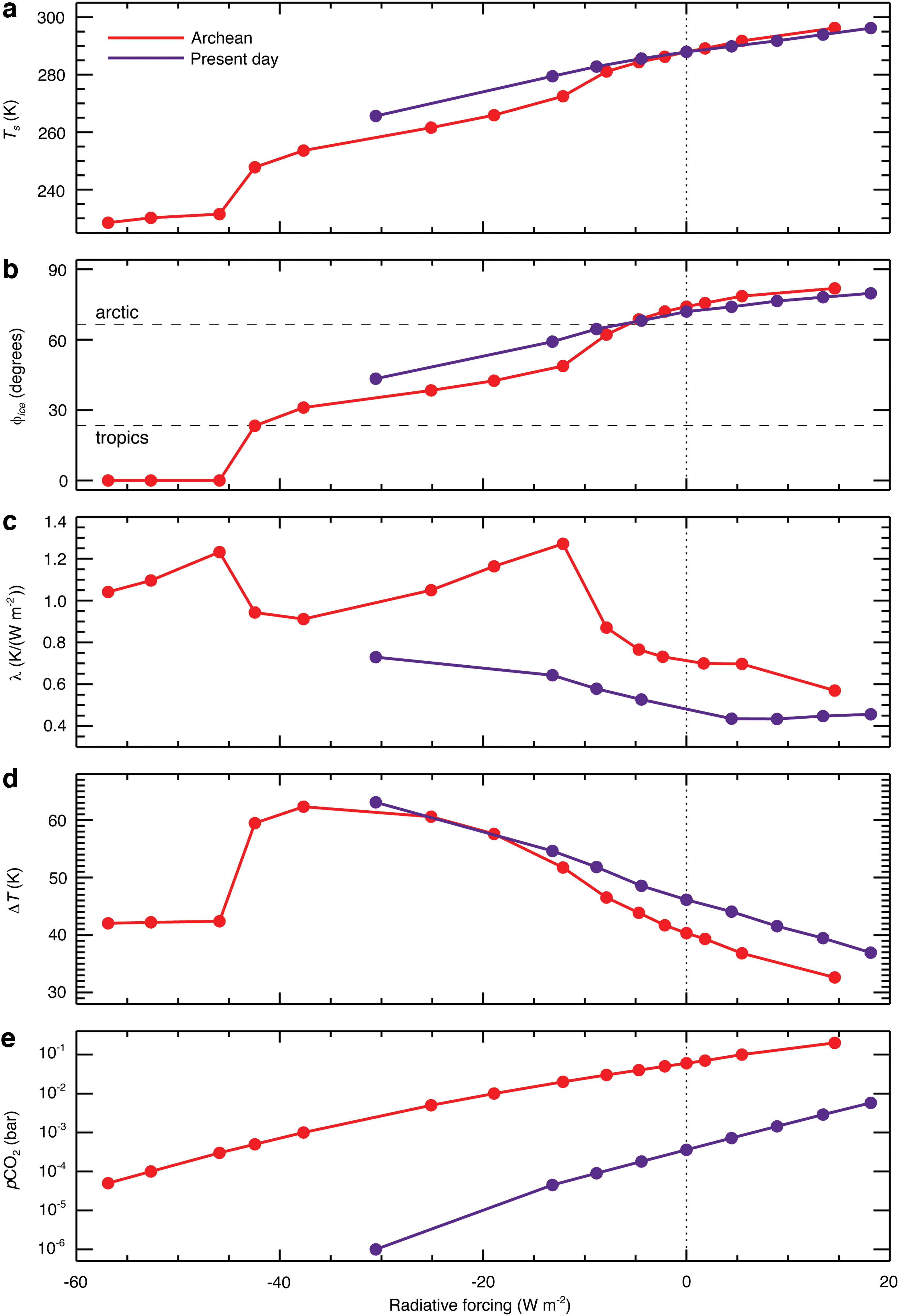
Climate response to changes in clear-sky radiative forcing at the tropopause under present-day and late Archean solar constants (1367.0 and 1093.6 W m⁻², respectively). Radiative forcings are applied by varying pCO₂ for the present day with oxygen and ozone (purple) and late Archean (red) simulations, referenced from standard atmospheres (see Table 2). A radiative forcing of zero (vertical dotted line) indicates standard atmospheric states for the late Archean and for present-day Earth, both having mean surface temperatures of 287.9 K. (a) Mean surface temperature (T _s) versus radiative forcing. (b) Annual and zonal mean sea ice margin (φ_ice) versus radiative forcing. The sea ice margin is calculated as the inverse sine of the global and annual mean open ocean fraction. (c) Archean climate sensitivities (λ) are larger and more complex compared with the present day. Maxima indicate tipping points between quasi-stable climate states. (d) Annual, zonal, and hemispheric mean meridional temperature differences (ΔT) between the tropics (22°) and the arctic (74°) versus radiative forcing. (e) CO₂ partial pressure versus radiative forcing. Color images available online at www.liebertonline.com/ast

The maxima in climate sensitivity in Fig. 7c centered at −12.1 W m⁻² marks a transition from a state where sea ice is confined to polar regions to a state where sea ice can extend into midlatitudes. The sharp increase in Archean climate sensitivity for radiative forcings between −5 and −12 W m⁻² is caused by fundamental changes to the latitudinal distribution of energy under a faint Sun and strong greenhouse. As mentioned above, our standard Archean atmosphere receives less radiant energy at the equatorial surface, while receiving more radiant energy at the poles compared with the present day (Fig. 3). This fundamental modulation of the latitudinal surface energy distribution causes Archean simulations with surface temperatures close to those of the present day to have reduced meridional temperature differences (Fig. 7d) and less sea ice (Fig. 7b) compared with simulations under the modern Sun. The meridional temperature difference shown in Fig. 7d is calculated as the annual, zonal, and hemispheric mean surface temperature difference between grid cells centered at 22° and 74° latitude. Reduced latitudinal temperature differences permit ice to advance (or retreat) more easily for a given radiative forcing (Pierrehumbert, 2002). In this study, a reduction in Archean pCO₂ from 0.03 to 0.02 bar, a radiative forcing of −4.3 W m⁻², causes an annual mean surface cooling of 8.6 K and an annual and hemispheric mean equatorward expansion of sea ice by 12° latitude. By contrast, for simulations of present-day Earth, reducing CO₂ from 360 to 180 ppm yields a nearly identical radiative forcing of −4.4 W m⁻²; however, mean surface cooling is only 2.3 K, and sea ice expands equatorward by only 2°. If Archean ice sheets are allowed to expand into the midlatitudes, mean surface temperatures plummet, meridional temperature differences increase due to polar amplification, and the ice-albedo feedback weakens. A larger meridional temperature gradient makes it more difficult to form ice at low latitudes for a given mean surface temperature (Pierrehumbert, 2002).

The maximum in climate sensitivity in Fig. 7c at −45.9 W m⁻² marks the final transition into a completely ice-covered world. In our model, this corresponds to a glaciation threshold between 300 and 500 ppm of CO₂ for the Archean climate. While at face value this is certainly an intriguing result, here the observed climate stability down to low CO₂ is likely attributed to the absence of a dynamical sea ice model. While plausible changes to ocean heat transport may only have a small effect on the tipping point toward runaway glaciation, the equatorward flow of sea ice is a key element in triggering a “snowball” Earth (Voigt and Abbot, 2012). Even so, GCMs that include dynamic oceans and sea ice still commonly find stable “waterbelt” climates with sea ice lines located in the tropics (Voigt and Abbot, 2012; Yang and Peltier, 2012; Yang et al., 2012). Furthermore, while we argue here that limitations of the Archean geological record make it inappropriate to preclude climates with relatively large polar ice caps compared with the present day, waterbelt climate states where the surface experiences glaciation covering 80% or more of the surface may stretch the believable limits for cold Archean climate solutions. Considering the limitations of our model, here we take a conservative approach and limit the scope of acceptable Archean climate solutions to those with stable sea ice margins poleward of 30° degrees latitude (i.e., with 50% open ocean or greater). Future studies in which coupled dynamic ocean and sea ice models are used should be employed to better estimate tipping points toward complete glaciation.

3.3. Hospitable Archean climates

Hospitable late Archean climates, dominated by open ocean, are permitted safely within constraints imposed on paleoatmospheric CO₂. Here, we have adopted the constraint of Driese et al. (2011), which limits paleoatmospheric CO₂ at 2.69 Ga to between 10 and 50 PAL (0.0036–0.018 bar), with a best-guess value of 41 PAL (∼0.015 bar). With 0.015 bar of CO₂ and no CH₄, the global mean surface temperature stays below freezing (Fig. 8a); however, surface temperatures averaged across the tropics reach 284 K (Fig. 8b), and the sea ice margin stabilizes at 46° latitude (Fig. 8c). In this case, ∼72% of the planet's surface area remains free from ice. With 0.015 bar of CO₂ and 0.001 bar of CH₄, the global mean surface temperature is 285 K while mean tropical surface temperatures reach 296 K, only a few degrees colder than the present day. The sea ice margin is stable at 68° latitude; thus ∼93% of the surface would remain free from ice. In this case, photochemical hazes would not be expected to form, since CH₄:CO₂<0.1. Thus a relatively warm, ocean-dominated late Archean poses no conflict with imposed constraints on greenhouse gases. Stable cooler climates with more extensive ice coverage are possible at lower CO₂ (and CH₄). Stable climates with 0.005 bar of CO₂ and no CH₄ are found having T _s=262 K and a sea ice margin at 38° latitude (∼62% of surface free from ice). In this case, increasing CO₂ from 360 ppm to 0.005 bar yields a radiative forcing of +16.9 W m⁻², while reductions to low clouds are compounded by cool surface temperatures resulting in a net cloud forcing of only −0.9 W m⁻², a gain of 24.0 W m⁻² at the tropopause compared with the present climate. A range of hospitable climate solutions exist with 0.005<pCO₂<0.015 bar, which have significant polar ice caps but are still dominated by open ocean. Within this range of paleoatmospheric CO₂, the addition of smaller amounts of methane (0.0001 bar or less) can contribute up to ∼6 K of further warming without initiating photochemical haze formation (Haqq-Misra et al., 2008). If we are allowed to consider climates with large polar ice caps as valid solutions, resolving the faint young Sun paradox within constraints on greenhouse gases becomes remarkably easy.

FIG. 8.

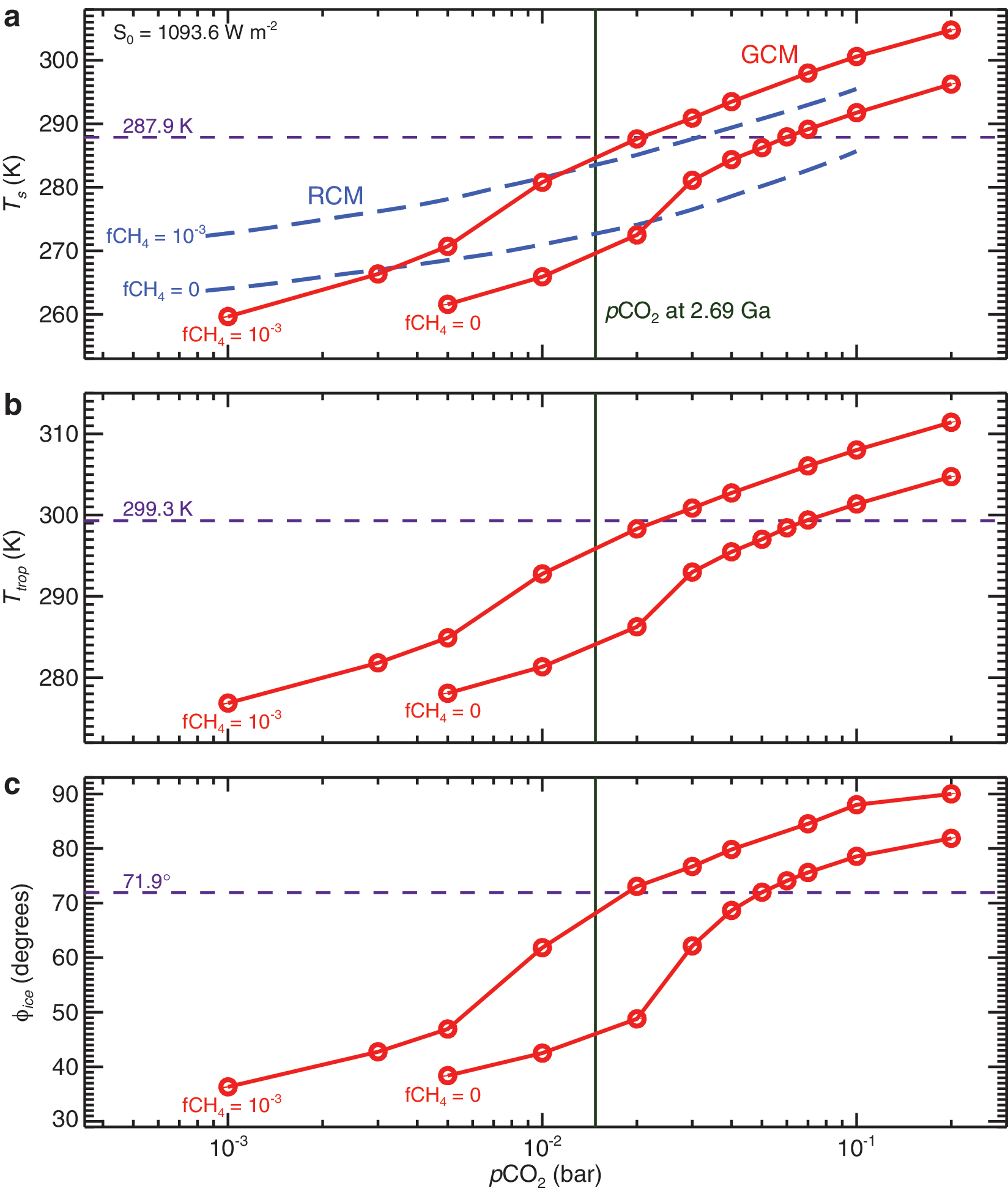
Archean climate response to varying CO₂ partial pressure. (a) Mean surface temperature (T _s) versus pCO₂ from this study (red) and from a recent RCM study (blue, Haqq-Misra et al., 2008) for 0 and 0.001 bar of CH₄, respectively, under 80% of the modern solar constant. A recent estimate for paleoatmospheric CO₂ abundance dated to 2.69 Ga is indicated at pCO₂=0.015 bar (green, Driese et al., 2011). (b) Mean tropical temperature (T _trop) between 22°S and 22°N latitudes for GCM simulations. (c) Annual and hemispheric mean sea ice margin (φ_ice) for GCM simulations. Purple dashed lines indicate the values from simulations of present-day climate. Color images available online at www.liebertonline.com/ast

Our Archean GCM exhibits greater sensitivity to changing CO₂ compared with published results from paleoclimate simulations utilizing one-dimensional RCMs (Haqq-Misra et al., 2008). This comes as no surprise since RCMs used for paleoclimate simulations typically set the surface albedo to a constant; thus ice-albedo and cloud feedbacks to changing surface temperature are not included (Kasting et al., 1984). Here, as expected, we find that the temperature versus pCO₂ curve is consistently steeper for GCM simulations than for RCM simulations (Fig. 8a). Nonetheless, the qualitative similarity between the model surface temperature responses from GCMs and RCMs (i.e., fairly smooth and lacking sharp bifurcations) is encouraging but also somewhat surprising. First-order differences between GCM and RCM simulated mean surface temperatures can be understood in terms of modulations to the albedo and cloud forcings (Fig. 9). RCMs parameterize the net radiative effect of clouds and ice within the surface albedo, typically setting it to a constant value of ∼0.22 in all simulations (Haqq-Misra et al., 2008). As CO₂ is reduced from 0.2 to 0.005 bar in our GCM, global mean surface temperatures fall from 296 to 262 K, the sea ice margin expands from 82° to 38° latitude, and the global mean surface albedo increases from 0.11 to 0.32. The difference in mean surface temperatures between GCM and RCM simulations mirrors the variation in surface albedo determined by our GCM relative to the constant value for surface albedo used in RCMs, which indicates the importance of the ice-albedo feedback (Fig. 9a). However, cloudiness and Rayleigh scattering moderate the contribution of the surface albedo to the TOA albedo. Both cloud and Rayleigh scattering albedos act to oppose increases to the surface albedo as CO₂ and surface temperature analogously decrease. Rayleigh scattering is directly related to the atmospheric CO₂ content. The global mean cloud albedo varies with surface temperature. On a cold Archean world the hydrological cycle weakens because the saturation vapor pressure varies sharply with temperature. Optically thick water clouds are eliminated in favor of tenuous ice clouds. While the longwave cloud forcing remains relatively constant, the shortwave and net cloud forcings decrease in magnitude with decreasing surface temperature (Fig. 9b). The persistence of ice clouds (vis-à-vis liquid clouds) as the climate cools serves as a buffer against runaway glaciation for cold early climates in support of earlier theories (Rossow et al., 1982). However, here this effect is weak and does not provide a full solution to the faint young Sun paradox. As the planet cools, a larger percentage of the total greenhouse effect comes from clouds rather than from gaseous absorption. For colder climates, 20% or more of the total greenhouse effect can come from ice clouds, while for Archean climates with temperatures near those of the present day (boosted by CO₂), ice clouds contribute slightly more than 12% of the total greenhouse (Fig. 9c). Combining effects of surface, cloud, and atmosphere, the TOA albedo exhibits a much more modest increase (0.31–0.42) than does the surface albedo over our range in climate. RCMs change neither surface nor cloud albedo and therefore accidentally benefit from their partial cancellation, allowing RCM and GCM temperature curves to remain surprisingly similar despite the use of vastly different methods.

FIG. 9.

(a) Global mean TOA, surface, cloud, and Rayleigh scattering albedos vs. atmospheric CO₂ for Archean simulations, analogous with Fig. 8. Radiative-convective models typically use an effective surface albedo of ∼0.22 to implicitly incorporate cloud forcings. (b) Cloud longwave, shortwave, and net forcing at the tropopause vs. atmospheric CO₂. (c) Percent contribution of gaseous and cloud absorption to the total greenhouse effect. Color images available online at www.liebertonline.com/ast

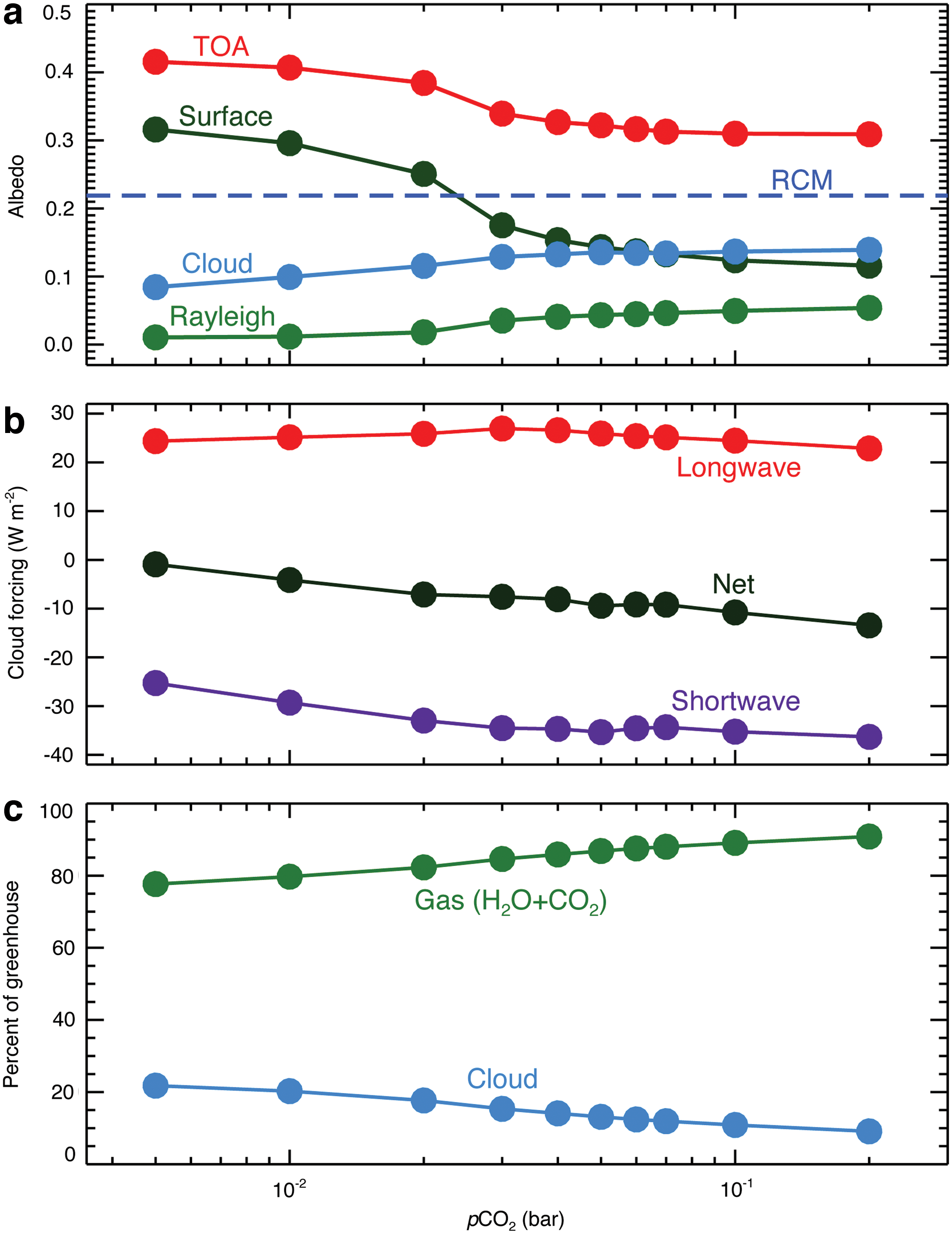
An often overlooked shortcoming of RCM paleoclimate studies is that they typically assume that if the mean surface temperature falls below 273 K (Domagal-Goldman et al., 2008; Haqq-Misra et al., 2008) or sometimes 279 K (Goldblatt et al., 2009b), runaway glaciation to a hard snowball will be the inevitable result. However, in this study a sharp bifurcation to a frozen world is not observed when T _s drops below 273 K. Here, we find stable climates with T _s as low as 260 K that maintain open ocean fractions of greater than 50%. Similar climate solutions with T _s<273 K but with open oceans at low latitudes and midlatitudes are also commonly found in GCMs that use more complex treatments of oceans and sea ice albeit within the context of different geological epochs and radiative forcings (Voigt et al., 2011; Voigt and Abbot, 2012; Yang and Peltier, 2012; Yang et al., 2012). Stable climates may even be possible with sea ice margins as low as 10° to 20° latitude and global mean surface temperatures well below freezing (Abbot et al., 2011; Yang et al., 2012). RCMs remain attractive research tools since they are computationally fast and can incorporate comprehensive self-consistent reducing atmospheric chemistry. The utility of paleoclimate RCMs may be expanded by incorporating simple cloud and ice-albedo feedback parameterizations and through the realization that solutions with T _s<273 K remain viable for a habitable early Earth with substantial liquid water at the surface.

4. Discussion

The isotopic composition of marine sediments commonly serves as a proxy for paleo-ocean temperatures. The oxygen and silicon isotopic composition of seawater and water-lain sediments is controlled by temperature-dependent exchange of ¹⁸O between water and rock within hydrothermal vent systems and mid-ocean ridges (Kasting et al., 2006). Taken at face value, low-δ¹⁸O and δ³⁰Si inclusions are interpreted as indicators of hot seawater temperatures, possibly reaching as high as 350 K during the late Archean (Knauth and Lowe, 2003; Robert and Chaussidon, 2006). However, observed low-δ¹⁸O signals found in Archean sediments may be the result of variations in hydrothermal fluid temperature through time rather than variations in the mean seawater temperature (Kasting et al., 2006; Shields and Kasting, 2007; van der Boorn et al., 2007). Observed isotopic data might reflect more widespread hydrothermal activity on the ancient seafloor, which slowly tapered off through time (Hofmann, 2005; van der Boorn et al., 2007). Enhanced continental weathering from higher paleoatmospheric CO₂ and a greater abundance of brittle volcanic rocks may have acted to suppress δ¹⁸O during the Precambrian (Jaffrés et al., 2007). Oceanic temperatures are also expected to vary strongly with latitude and depth. The paleolatitudes and depths of formation of the rocks on which the temperature estimates discussed above are based are unknown (Feulner, 2012). Some recent studies have improved upon traditional methods by conducting combined analysis of oxygen and hydrogen isotopes and by analyzing the oxygen isotopic composition of phosphates found in Archean sediments. These studies suggest that seawater temperatures during the mid-Archean were more moderate, likely between 299 and 308 K and no higher than 313 K (Hren et al., 2009; Blake et al., 2010).

In this study, our warmest Archean simulation, having 0.2 bar of CO₂ and 0.001 bar of CH₄ at 80% of the modern solar constant, exhibits global and annually averaged seawater temperatures that reach 305 K, while local seasonal maximum temperatures reach 321 K (Fig. 10). Coincidentally, this is also our only simulation that exhibits year-round ice-free conditions. While the seawater temperature predictions of Robert and Chaussidon (2006) are not reached in this study, the predictions of Blake et al. (2010) are achieved with reasonable greenhouse gas amounts. With 0.015 bar of CO₂ and 0.001 bar of CH₄, seasonal and local maximum seawater temperatures hover just above 305 K. With the inclusion of 0.001 bar of CH₄, our modeled seawater temperatures are in good agreement with recent estimates for paleo-ocean temperatures, while remaining safely within constraints imposed on paleoatmospheric CO₂.

FIG. 10.

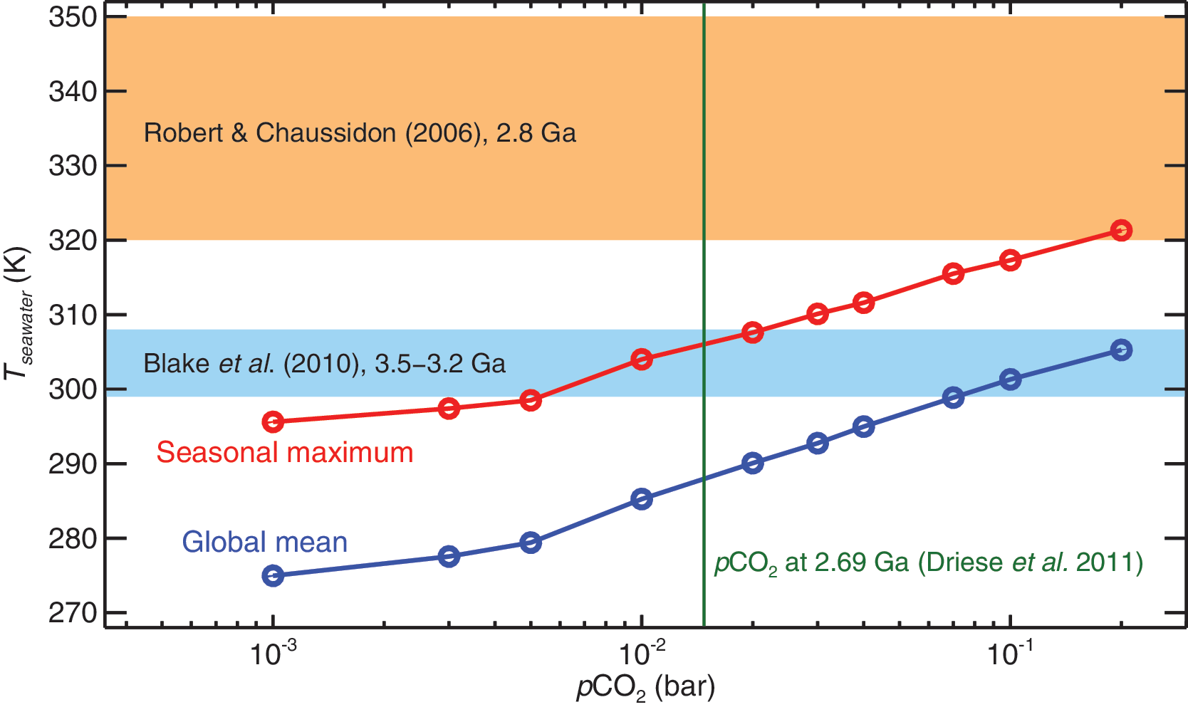
Seasonal maximum and global mean mixed-layer ocean temperature versus pCO₂ with 0.001 bar of CH₄ included. High seawater temperature estimates of Robert and Chaussidon (2006) are not possible within estimates of paleoatmospheric CO₂. However, our results can be easily reconciled with the more recent seawater temperature estimates of Blake et al. (2010). Color images available online at www.liebertonline.com/ast

A combination of high CO₂ and/or high CH₄ could in theory yield a hot climate for early Earth. However, large amounts of CO₂ (>0.2 bar) would be required to match the hot temperature estimates predicted by Knauth and Lowe (2003) and Robert and Chaussidon (2006) if CO₂ and H₂O were the only greenhouse gases, hopelessly violating inferred constraints on CO₂. Photochemical calculations of Zerkle et al. (2012) predict an upper limit on atmospheric methane obeying the ratio CH₄:CO₂=0.2. Thus, if the predicted atmospheric CO₂ at 2.69 Ga is 0.015 bar, CH₄ is limited to only 0.003 bar, 3 times what is presented in this study. However, such an increase in CH₄ would yield only a few additional watts per meter squared of radiative forcing (Fig. 1d), and that is before the radiative effects of organic hazes are even considered. A hot, dense, carbon-rich atmosphere would have left the scars of intense chemical weathering; however, the geological record suggests that weathering rates were modest during the Archean (Condie et al., 2001; Sleep and Hessler, 2006). Additionally, as one moves backward through geological time, the Sun becomes fainter; thus the climate would require increasingly large amounts of greenhouse gases to offset. For reference, at the onset of the Archean circa 3.8 Ga the Sun was only 75% as bright as it is today, which translates into an additional radiative forcing of −14.3 W m⁻² compared to simulations presented in this study.

An alternative to the hot ocean viewpoint is that the Archean had a more temperate climate. A temperate Archean is more easily reconcilable with evidence for glaciations observed around 2.3 Ga (Evans et al., 1997) and 2.9 Ga (Young et al., 1998) as opposed to an excessively hot planet. A transition from a hot, ice-free state to a hard snowball state requires large radiative forcings and exhibits a strong hysteresis (Pierrehumbert, 2004). By contrast, a temperate Archean may have easily swayed into and out of more moderate glacial states, not unlike the climate of more recent epochs. Here, we find the Archean climate to have a greater sensitivity than the present day; thus a relatively small push on the radiative balance can transition a temperate late Archean climate from one where ice is confined to polar regions to one where ice extends into midlatitudes. The interaction of methane, biology, and photochemical hazes may be responsible for Archean climate changes. Thickening photochemical hazes from increased methanogenic respiration may have been responsible for the lesser glaciation believed to have occurred at 2.9 Ga (Domagal-Goldman et al., 2008). Assuming fractal-shaped haze particles, Zerkle et al. (2012) predicted that haze effective optical depths at 0.550 μm reach 0.3 when methane reaches CH₄:CO₂=0.2. Such a haze would extinguish more than a quarter of the incoming solar energy. The glaciation at the end of the Archean circa 2.4 Ga is widely speculated to have been caused by the rise of oxygen and the subsequent destruction of a methane greenhouse (Kasting, 2005). If the preglacial atmosphere contained 0.015 bar of CO₂, the loss of 0.001 bar of methane due to rising oxygen levels would yield a ∼15 K global mean temperature decline and a ∼23° latitudinal expansion of sea ice. Even larger temperature changes would have occurred if higher CH₄ concentrations had been present prior to the rise of oxygen.

5. Conclusions

Here, we have used a GCM to study the climate of the late Archean circa 2.8 Ga when the Sun was 20% dimmer than in the present day. We find self-consistent climate solutions to a weaker form of the faint young Sun paradox, requiring that only some portion of the planet's surface remain free from ice and thus hospitable for early life. While self-consistent hot solutions for the late Archean remain elusive, we find that cooler climates that remain dominated by areas of liquid surface water are easily achieved within published paleoatmospheric constraints on CO₂. The combination of 0.015 bar of CO₂ and 0.001 bar of CH₄ produces surface temperatures very near those of the present day, while not violating paleosol constraints on CO₂ and avoiding complications from photochemical haze formation. Climates with weaker greenhouses and mean surface temperatures as low as 260 K can maintain open ocean fractions of greater than 50%, thus ensuring the habitability of the Archean even at relatively low paleoatmospheric greenhouse gas levels. Convincing geological arguments can be made in favor of a more temperate late Archean climate as opposed to an excessively hot planet. One need not extrapolate based on sparse geological data to there being only climates of extreme hot and cold during the Archean. The change in latitudinal energy distribution compared with the present day due to weak solar irradiance and a strong greenhouse effect may have caused the ancient climate to be susceptible to wide swings for relatively small radiative forcings. However, here climates with open ocean fractions of greater than 50% are maintained despite a 20% reduction in the solar constant even with only 0.005 bar of CO₂ and no CH₄. Additional mechanisms not included in this study such as a decrease in the number of cloud condensation nuclei (Rosing et al., 2010), decreased emergent continental crust (Rosing et al., 2010), an increased rotation rate (Jenkins et al., 1993), increased N₂ (Goldblatt et al., 2009b), and the inclusion of additional trace greenhouse species (Sagan and Mullen, 1972; Haqq-Misra et al., 2008; Ueno et al., 2009) may result in even warmer temperatures than are presented here. Resolving the faint young Sun paradox may not be as challenging to climate modelers as previously thought.

Footnotes

Acknowledgments

We thank NASA Earth and Space Science Fellowship award NNX10AR97H and NASA Exobiology award NNX10AR17G for financial support. This work utilized the Janus supercomputer, which is supported by the National Science Foundation (award number CNS-0821794) and the University of Colorado at Boulder. We also thank F. Forget and D. Koll for helpful reviews of this manuscript.

Author Disclosure Statement

No competing financial interests exist.

Abbreviations

CAM3, Community Atmosphere Model version 3.0; GCM, general circulation model; LBLRTM, line-by-line radiative transfer model; PAL, present atmospheric level; RCM, radiative-convective model; TOA, top-of-atmosphere.

References

Abbot

D.S.

, Voigt

, Koll

2011. The Jormungand global climate state and implications for Neoproterozoic glaciations. J Geophys Res, 116. 10.1029/2011JD015927.

Allwood

A.C.

, Walter

M.R.

, Kamber

B.S.

, Burch

I.W.

2006. Stromatolite reef from the Early Archaean era of Australia. Nature, 414:714–718.

Barker

H.W.

, Cole

J.N.S

, Morcrette

J.-J.

, Pincus

, Räisänen

, von Salzen

, Vaillancourt

P.A.

2008. The Monte Carlo Independent Column Approximation: an assessment using several global atmospheric models. Quarterly Journal of the Royal Meteorological Society, 134:1463–1478.

Blake

R.E.

, Chang

S.J.

, Lepland

2010. Phosphate oxygen isotopic evidence for a temperate and biologically active Archaean ocean. Nature, 464:1029–1033.

Briegleb

B.P.

, Bitz

C.M.

, Hunke

E.C.

, Lipscomb

W.H.

, Holland

M.N.

, Schramm

J.L.

, Moritz

R.E.

2004. Scientific Description of the Sea Ice Component in the Community Climate System Model, Version Three, NCAR Technical Note/TN-463+STR. National Center for Atmospheric Research: Boulder, CO http://www.cesm.ucar.edu/models/ccsm3.0/csim/SciGuide/tech_note_23jun04_release.ps

Clough

S.A.

, Shephard

M.W.

, Mlawer

E.J.

, Delamere

J.S.

, Iacono

M.J.

, Cady-Pereira

, Boukabara

, Brown

P.D.

2005. Atmospheric radiative transfer modeling: a summary of the AER codes. J Quant Spectrosc Radiat Transf, 91:233–244.

Collins

W.D.

, Rasch

P.J.

, Boville

B.A.

, Hack

J.J.

, McCaa

J.R.

, Williamson

D.L.

, Kiehl

J.T.

, Briegleb

, Bitz

, Lin

S.-J.

, Zhang

, Dai

2004. Description of the NCAR Community Atmosphere Model (CAM 3.0), NCAR Technical Note/TN-464+STR. National Center for Atmospheric Research: Boulder, CO http://www.cesm.ucar.edu/models/atm-cam/docs/description/description.pdf

Collins

W.D.

, Rasch

P.J.

, Boville

B.A.

, Hack

J.J.

, McCaa

J.R.

, Williamson

D.L.

, Briegleb

B.P.

2006. The formulation and atmospheric simulation of the Community Atmosphere Model Version 3 (CAM3) J Clim, 19:2144–2161.

Condie

K.C.

, DesMarais

D.J.

, Abbott

2001. Precambrian superplumes and supercontinents: a record in black shales, carbon isotopes, and paleoclimates? Precambrian Res, 106:239–260.

10.

Dauphas

, Kasting

J.F.

2011. Low pCO₂ in the pore water, not in the Archean air. Nature, 474. 10.1038/nature09960.

11.

DeWitt

H.L.

, Trainer

M.G.

, Pavlov

A.A.

, Hasenkopf

C.A.

, Aiken

A.C.

, Jimenez

J.L.

, McKay

C.P.

, Toon

O.B.

, Tolbert

M.A.

2009. Reduction in haze formation rate of prebiotic Earth in the presence of hydrogen. Astrobiology, 9:447–453.

12.

Dhuime

, Hawkesworthm

C.J.

, Cawood

P.A.

, Storey

C.D.

2012. A change in the geodynamics of continental growth 3 billion years ago. Science, 335:1334–1336.

13.

Domagal-Goldman

S.D.

, Kasting

J.F.

, Johnston

D.T.

, Farquhar

2008. Organic haze, glaciations and multiple sulfur isotopes in the Mid-Archean era. Earth Planet Sci Lett, 269:29–40.

14.

Driese

S.G.

, Jirsa

M.A.

, Ren

, Brantley

S.L.

, Sheldon

N.D.

, Parker

, Schmitz

2011. Neoarchean paleoweathering of tonalite and metabasalt: implications for reconstructions of 2.69 Ga early terrestrial ecosystems and paleoatmospheric chemistry. Precambrian Res, 189:1–17.

15.

Evans

D.A.

, Beukes

N.J.

, Kirshvink

J.L.

1997. Low-latitude glaciation in the Proterozoic era. Nature, 386:262–266.

16.

Feulner

2012. The faint young Sun problem. Rev Geophys, 50. 10.1029/2011RG000375.

17.

Ferreira

, Marshall

, Rose

2011. Climate determinism revisited: multiple equilibria in a complex climate model. J Clim, 24:992–1012.

18.

Fomichev

V.I.

, Blanchet

J.-P.

, Turner

D.S.

1998. Matrix parameterization of the 15 μm CO₂ band cooling in the middle and upper atmosphere for variable CO₂ concentration. J Geophys Res, 103:11505–11528.

19.

Goldblatt

, Zahnle

K.J.

2011. Clouds and the faint young Sun paradox. Climate of the Past, 7:203–220.

20.

Goldblatt

, Lenton

T.M.

, Watson

A.J.

2009a. An evaluation of the long-wave radiative transfer code used in the Met Office Unified Model. Quarterly Journal of the Royal Meteorological Society, 134:619–633.

21.

Goldblatt

, Claire

M.W.

, Lenton

T.M.

, Matthews

A.J.

, Watson

A.J.

, Zahnle

K.J.

2009b. Nitrogen-enhanced greenhouse warming on early Earth. Nat Geosci, 2:891–896.

22.

Gough

D.O.

1981. Solar interior structure and luminosity variations. Solar Physics, 74:21–34.

23.

Halevy

, Pierrehumbert

R.T.

, Schrag

D.P.

2009. Radiative transfer in CO₂-rich paleoatmospheres. J Geophys Res, 114. 10.1029/2009JD011915.

24.

Hansen

, Sato

, Ruedy

, Nazarenko

, Lacis

, Schmidt

G.A.

, Russell

, Aleinov

, Bauer

, Bell

, Cairns

, Canuto

, Chandler

, Cheng

, Del Genio

, Faluvegi

, Fleming

, Friend

, Hall

, Jackman

, Kelley

, Kiang

, Koch

, Lean

, Lerner

, Lo

, Menon

, Miller

, Minnis

, Novakov

, Oinas

, Perlwitz

Ja.

, Perlwitz

Ju.

, Rind

, Romanou

, Shindell

, Stone

, Sun

, Tausnev

, Thresher

, Wielicki

, Wong

, Yao

, Zhang

2005. Efficacy of climate forcings. J Geophys Res, 110. 10.1029/2005JD005776.

25.

Haqq-Misra

J.D.

, Domagal-Goldman

S.D.

, Kasting

P.J.

, Kasting

J.F.

2008. A revised, hazy methane greenhouse for the Archean Earth. Astrobiology, 8:1127–1137.

26.

Henderson-Sellers

, Henderson-Sellers

1988. Equable climate in the early Archean. Nature, 336:117–118.

27.

Hofmann

2005. The geochemistry of sedimentary rocks from the Fig Tree Group, Barberton greenstone belt: implications for tectonic, hydrothermal and surface processes during mid-Archaean times. Precambrian Res, 143:23–49.

28.

Hren

M.T.

, Tice

M.M.

, Chamberlain

C.P.

2009. Oxygen and hydrogen isotope evidence for a temperate climate 3.42 billion years ago. Nature, 462:205–208.

29.

Hurrell

J.W.

, Hack

J.J.

, Phillips

A.S.

, Caron

, Yin

2006. The dynamical simulation of the Community Atmosphere Model Version 3 (CAM3) J Clim, 19:2162–2183.

30.

Jaffrés

J.B.D.

, Shields

G.A.

, Wallmann

2007. The oxygen isotope evolution of seawater: a critical review of a long-standing controversy and an improved geological water cycle model for the past 3.4 billion years. Earth-Science Reviews, 83:83–122.

31.

Jenkins

G.S.

1993. A general circulation model study of the effects of faster rotation rate, enhanced CO₂ concentration, and reduced solar forcing: implications for the faint young Sun paradox. J Geophys Res, 98:20803–20811.

32.

Jenkins

G.S.

2001. High-obliquity simulations for the Archean Earth: implications for climatic conditions on early Mars. J Geophys Res, 106:32903–32913.

33.

Jenkins

G.S.

, Marshall

H.G.

, Kuhn

W.R.

1993. Precambrian climate: the effects of land area and Earth's rotation rate. J Geophys Res, 98:8785–8791.

34.

Kasting

J.F.

1987. Theoretical constraints on oxygen and carbon dioxide concentrations in the Precambrian atmosphere. Precambrian Res, 34:205–229.

35.

Kasting

J.F.

2005. Methane and climate during the Precambrian era. Precambrian Res, 137:119–129.

36.

Kasting

J.F.

2010. Faint young Sun redux. Nature, 464:687–689.

37.

Kasting

J.F.

, Pollack

J.B.

, Crisp

. 1984. Effects of high CO₂ levels on surface temperature and atmospheric oxidation state of the early Earth. J Atmos Chem, 1:403–428.

38.

Kasting

J.F.

, Howard

M.T.

, Wallmann

, Veizer

, Shields

, Jaffrés

2006. Paleoclimates, ocean depth, and the oxygen isotopic composition of seawater. Earth Planet Sci Lett, 252:82–93.

39.

Kharecha

, Kasting

, Siefert

2005. A coupled atmosphere-ecosystem model of the early Archean Earth. Geobiology, 3:53–76.

40.

Kienert

, Feulner

, Petoukhov

2012. Faint young Sun problem more severe due to ice-albedo feedback and higher rotation rate of the early Earth. Geophys Res Lett, 39. 10.1029/2012GL054381.

41.

Klein

S.A.

, Hartmann

D.L.

1993. The seasonal cycle of low stratiform clouds. J Clim, 6:1587–1606.

42.

Knauth

L.P.

, Lowe

D.R.

2003. High Archean climatic temperature inferred from oxygen isotope geochemistry of cherts in the 3.5 Ga Swaziland Supergroup, South Africa. Geol Soc Am Bull, 115:566–580.

43.

Lin

S.J.

, Rood

R.B.

1996. Multidimensional flux-form semi-Lagrangian transport schemes. Monthly Weather Review, 124:2046–2070.

44.

Mengel

, Short

, North

1988. Seasonal snowline instability in an energy balance model. Climate Dynamics, 2:127–131.

45.

Mlawer

E.J.

, Taubman

S.J.

, Brown

P.D.

, Iacono

M.J.

, Clough

S.A.

1997. Radiative transfer for inhomogeneous atmospheres: RRTM, a validated correlated-k model for the longwave. J Geophys Res, 102:16663–16682.

46.

Mojzsis

S.J.

, Arrhenius

, McKeegan

K.D.

, Harrison

T.M.

, Nutma

A.P.

, Friend

C.R.L.

1996. Evidence for life on Earth before 3,800 million years ago. Nature, 384:55–59.

47.

Pierrehumbert

R.T.

2002. The hydrologic cycle in deep-time climate problems. Nature, 419:191–198.

48.

Pierrehumbert

R.T.

2004. High levels of atmospheric carbon dioxide necessary for the termination of global glaciation. Nature, 429:646–649.

49.

Pincus

, Barker

H.W.

, Morcrette

2003. A fast, flexible, approximate technique for computing radiative transfer in inhomogeneous cloud fields. J Geophys Res, 108. 10.1029/2002JD003322.

50.

Poulsen

C.J.

, Pierrehumbert

R.T.

, Jacob

2001. Impact of ocean dynamics on the simulation of the Neoproterozoic “Snowball Earth.” Geophys Res Lett, 28:1575–1578.

51.

Rasch

P.J.

, Kristjánsson

J.E.

1998. A comparison of the CCM3 model climate using diagnosed and predicted condensate parameterizations. J Clim, 11:1587–1614.

52.

Reinhard

C.T.

, Planavsky

N.J.

2011. Mineralogical constraints on Precambrian pCO₂ . Nature, 474. 10.1038/nature09959.

53.

Robert

, Chaussidon

2006. A paleotemperature curve for the Precambrian oceans based on silicon isotopes in cherts. Nature, 443:969–972.

54.

Rondanelli

, Lindzen

R.S.

2010. Can thin cirrus clouds in the tropics provide a solution to the faint young Sun paradox? J Geophys Res, 115. 10.1029/2009JD012050.

55.

Rosing

M.T.

1999. ¹³C-depleted carbon in >3700 Ma seafloor sedimentary rocks from West Greenland. Science, 283:674–676.

56.

Rosing

M.T.

, Bird

D.K.

, Sleep

N.H.

, Bjerrum

C.J.

2010. No climate paradox under the faint early Sun. Nature, 464:744–747.

57.

Rossow

W.B.

, Sellers

A.H.

, Weinreich

S.K.

1982. Cloud feedback: a stabilizing effect for the early Earth? Science, 217:1245–1247.

58.

Rothman

L.S.

, Jacquemart

, Barbe

, Chris Benner

, Birk

, Brown

L.R.

, Carleer

M.R.

, Chackerian

Jr. , Chance

, Coudert

L.H.

, Dana

, Devi

V.M.

, Flaud

J.-M.

, Gamache

R.R.

, Goldman

, Hartmann

J.-M.

, Jucks

K.W.

, Maki

A.G.

, Mandin

J.-Y.

, Massie

S.T.

, Orphal

, Perrin

, Rinsland

C.P.

, Smith

M.A.H.

, Tennyson

, Tolchenov

R.N.

, Toth

R.A.

, Vander Auwera

, Varanasi

, Wagner

2005. The HITRAN 2004 molecular spectroscopic database. J Quant Spectrosc Radiat Transf, 96:139–204.

59.

Rye

, Kuo

P.H.

, Holland

H.D.

1995. Atmospheric carbon dioxide concentrations before 2.2 billion years ago. Nature, 378:603–605.

60.

Sagan

, Mullen

1972. Evolution of atmospheres and surface temperatures. Science, 276:52–56.

61.

Schopf

J.W.

2006. Fossil evidence for Archaean life. Philos Trans R Soc Lond B Biol Sci, 361:869–885.

62.

Sheldon

N.D.

2006. Precambrian paleosols and atmospheric CO₂ levels. Precambrian Res, 147:148–155.

63.

Shi

, Xu

, Wang

, Dai

, Zhao

2009. An improved treatment of overlapping absorption bands based on the correlated k distribution model for thermal infrared radiative transfer calculations. J Quant Spectrosc Radiat Transf, 110:435–451.

64.

Shields

G.A.

, Kasting

J.F.

2007. Evidence for hot early oceans? Nature, 447:E1–E2.

65.

Sleep

N.H.

, Hessler

A.M.

2006. Weathering of quartz as an Archean climatic indicator. Earth Planet Sci Lett, 241:594–602.

66.

Som

S.M.

, Catling

D.C.

, Harnmeijer

J.P.

, Polivka

P.M.

, Buick

2012. Air density 2.7 billion years ago limited to less than twice modern levels by fossil raindrop imprints. Nature, 484:359–362.

67.

Stone

P.H.

, Yao

M.S.

2004. The ice-covered Earth instability in a model of intermediate complexity. Climate Dynamics, 22:815–822.

68.

Tice

M.M.

, Lowe

D.R.

2004. Photosynthetic microbial mats in the 3,416-Myr-old ocean. Nature, 431:549–552.

69.

Toon

O.B.

, McKay

C.P.

, Ackerman

T.P.

, Santhanam

1989. Rapid calculation of radiative heating rates and photodissociation rates in inhomogeneous multiple scattering atmospheres. J Geophys Res, 94:16287–16301.

70.

Ueno

, Johnson

M.S.

, Danielache

S.O.

, Eskebjerg

, Pandey

, Yoshida

2009. Geological sulfur isotopes indicate elevated OCS in the Archean atmosphere, solving faint young Sun paradox. Proc Natl Acad Sci USA, 106:14784–14789.

71.

van der Boorn

, van Bergen

M.J.

, Nijman

, Vroon

P.Z.

2007. Dual role of seawater and hydrothermal fluids in Early Archean chert formation: evidence from silicon isotopes. Geology, 35:939–942.

72.

Vardavas

I.M.

, Carver

J.H.

1984. Solar and terrestrial parameterizations for radiative-convective models. Planet Space Sci, 32:1307–1325.

73.

Voigt

, Abbot

D.S.

2012. Sea-ice dynamics strongly promote Snowball Earth initiation and destabilize tropical sea-ice margins. Climate of the Past, 8:2079–2092.

74.

Voigt

, Abbot

D.S.

, Pierrehumbert

R.T.

, Marotzke

2011. Initiation of a Marinoan Snowball Earth in a state-of-the-art atmosphere-ocean general circulation model. Climate of the Past, 7:249–263.

75.

von Paris

, Rauer

, Grenfell

J.L.

, Patzer

, Hedelt

, Stracke

, Trautmann

, Schreier

2008. Warming the early Earth—CO₂ reconsidered. Planet Space Sci, 56:1244–1259.

76.

Wordsworth

, Pierrehumbert

2013. Hydrogen-nitrogen greenhouse warming in Earth's early atmosphere. Science, 339:64–67.

77.

World Meteorological Organization. 1957. Meteorology: a three-dimensional science, second session of the commission for aerology. WMO Bulletin, 6:134–138.

78.

K.M.

, Krueger

S.K.

1991. Evaluation of cloudiness parameterizations using a cumulus ensemble model. Monthly Weather Review, 119:342–367.

79.

Yang

, Peltier

W.R.

2012. The initiation of modern soft and hard Snowball Earth climates in CCSM4. Climate of the Past, 8:907–918.

80.

Yang

, Peltier

W.R.

, Hu

2012. The initiation of modern “Soft Snowball” and “Hard Snowball” climates in CCSM3. Part I: the influences of solar luminosity, CO₂ concentration, and the sea ice/snow albedo parameterization. J Clim, 25:2711–2736.

81.

Young

G.M.

, von Brunn

, Gold

D.J.C.

, Minter

W.E.L.

1998. Earth's oldest reported glaciation: physical and chemical evidence from the Archean Mozaan Group (∼2.9 Ga) of South Africa. J Geol, 106:523–538.

82.

Zerkle

A.L.

, Claire

M.W.

, Domagal-Goldman

S.D.

, Farquhar

, Poulton

S.W.

2012. A bistable organic-rich atmosphere on the Neoarchean Earth. Nat Geosci, 5:359–363.