Single-Photon Technique for the Detection of Periodic Extraterrestrial Laser Pulses

Abstract

To draw humankind's attention to its existence, an extraterrestrial civilization could well direct periodic laser pulses toward Earth. We developed a technique capable of detecting a quasi-periodic light signal with an average of less than one photon per pulse within a measurement time of a few tens of milliseconds in the presence of the radiation emitted by an exoplanet's host star. Each of the electronic events produced by one or more single-photon avalanche detectors is tagged with precise time-of-arrival information and stored. From this we compute a histogram displaying the frequency of event-time differences in classes with bin widths on the order of a nanosecond. The existence of periodic laser pulses manifests itself in histogram peaks regularly spaced at multiples of the—a priori unknown—pulse repetition frequency. With laser sources simulating both the pulse source and the background radiation, we tested a detection system in the laboratory at a wavelength of 850 nm. We present histograms obtained from various recorded data sequences with the number of photons per pulse, the background photons per pulse period, and the recording time as main parameters. We then simulated a periodic signal hypothetically generated on a planet orbiting a G2V-type star (distance to Earth 500 light-years) and show that the technique is capable of detecting the signal even if the received pulses carry as little as one photon on average on top of the star's background light. Key Words: Optical search for extraterrestrial intelligence—SETI—Single-photon detection—Detection of periodic laser signals. Astrobiology 13, 521–535.

1. Introduction

I n the first days of searching for extraterrestrial intelligence, it was assumed that the hydrogen-related wavelength near 21 cm would be the most likely carrier for interstellar communication. Meanwhile, the spectral region for this search has been broadened to include other microwave and radio frequencies, but no unambiguous extraterrestrial signal1 has been detected yet. The famous “WOW” signal, claimed to be detected on August 15, 1977, at the Big Ear Radio Telescope/Ohio State University Radio Observatory (Ehman, 2010), was a single irreproducible event and probably caused by human sources. Shortly after the invention of the laser, it was pointed out that spatially coherent light will allow transmitting messages over enormous distances in free space and thus could be used as an information carrier to and from extraterrestrials (Schwartz and Townes, 1961). It is straightforward to show that, with 10 m telescopes serving as transmit and receive antenna, respectively, and with laser pulses of 1.4 kJ energy, one will still receive one photon per pulse at a distance of 500 ly. (For this estimate we assumed a wavelength of λ=1 μm and transmission losses of 50%.) From a G2V-type star (such as the Sun) at the same distance, a 10 m telescope will collect only about 15 photons μs⁻¹ in a spectral band of 100 nm centered at λ=1 μm. This flux of photons would constitute a lower limit of background radiation from which the faint laser pulse would have to be distinguished.

A few groups have searched for extraterrestrial optical pulses of unnatural origin. The most elaborate published work refers to facilities installed at Harvard and Princeton, where more than 10,000 solar-type stars were targeted over several years (Howard et al., 2004). The capabilities of their instruments allowed them to identify 5 ns long pulses consisting of at least 80–100 photons m⁻² in the wavelength range 0.45 μm<λ<0.65 μm. The opto-electronic equipment relied on a beam splitter, two hybrid avalanche photodiodes, and electronics for coarse waveform reconstruction, and looked for coincidence of pulses in both channels. Simultaneous operation of two distant observatories allowed checking for synchronously occurring events. Despite the large number of stars observed using 1.5 and 0.9 m telescopes, no evidence for extraterrestrial laser signals was found. Later, the detection equipment was upgraded by incorporating two times 8 photomultipliers with 64 pixels each (Howard, 2006; Howard et al., 2007). With two times 512 pixels imaging the sky, the system allowed an all-sky search within reasonable time. But again, and so far, no unambiguous coincident optical signals were detected.

To reduce false-alarm probability, another experiment developed for the Lick Observatory consisted of even three optically parallel photomultipliers followed by coincident-detection electronics (Wright et al., 2001; Stone et al., 2005). The targeted search with a 1 m telescope extended over more than 4 years, with a dwell time of 10 min per star. At the University of Western Sydney, Australia, a 0.4 m and a 0.6 m telescope have been paired to look for the coincidence of nanosecond laser pulses—but without positive results (Bhathal, 2001).

An installation built for solar power research and high-energy gamma-ray astronomy was intentionally “misused” to look for blue-green laser pulses in the vicinity of some 200 stars at 200–800 ly distance (Hanna et al., 2009). A total of 224 heliostats provided an overall collecting area of 2300 m². However, the large field of view of 0.6 degrees necessitated a sophisticated coincident-detecting circuitry among the 64 photomultipliers serving as detectors to sufficiently eliminate background radiation. Despite a system sensitivity of 10 photons m⁻², no evidence for extraterrestrial laser pulses was found.

We explore a different route toward the detection of artificial extraterrestrial optical pulses. Our approach focuses on the detection of periodic signals when received over a sufficiently large number of cycles (Brunner et al., 2011). Repetitive optical pulses of high energy, repetition frequencies in the kilohertz regime and above, and little time jitter can be generated easily with solid state lasers. Such a pulse chain represents a signal not likely to be generated by a natural source. Its detection would thus be a hint for extraterrestrial intelligent origin. Moreover, because of the a priori periodicity, it can be distinguished from noise if very low (average) photon numbers are received and even if a large portion of the transmitted pulses is lost in a random manner on their way to the receiving station.

In this paper, we will start by accounting for the characteristics and parameters of the optical pulse chain we expect to receive from an extraterrestrial civilization. Together with background noise this will form the input signal from which we aim to retrieve the faint periodic extraterrestrial signal. Section 3 first presents the concept of the detection equipment, which is based on single-photon avalanche detectors and on time-tagging each detected photon. This is followed by a description of the fiber-coupled hardware actually used in our laboratory tests. In Section 4, we introduce strategies to recover the sought-for periodicity from sequences of time events, that is, from the recorded electronic pulses caused by photons and electronic noise. Here, we also discuss the pros and cons of splitting up the incoming photons and using several detectors in parallel. To test the equipment, we set up an optical source in which a faint periodic laser signal is superimposed with continuous optical background radiation. This allows us to record data sequences with varying parameters (Section 5). Examples of the result of the data analyses are presented in Section 6 in the form of histograms. They demonstrate that the overall concept allows identifying periodic signals in low signal-to-noise situations, even if the measurement time for a data sequence is as low as tens of milliseconds. Section 7 further substantiates the usefulness of the method devised by a computer simulation of the case of an input signal generated at an exoplanet orbiting a G2V-type star (distance to Earth 500 ly). Appendix A presents a simple model for predicting the approximate appearance of the histograms, as it will depend on the optical input parameters and the histogram parameters chosen.

2. Assumed Characteristics of Optical Input Signal

The design of an efficient detection scheme for faint electromagnetic signals is more difficult the less the designer knows about the signal to be detected. In the case of searching for periodic pulses intentionally transmitted by extraterrestrial intelligence, researchers have almost no hints concerning the signal parameters. One resort is to ask ourselves how we would design and realize a transmitter intended to draw the attention of extraterrestrial intelligence to our planet Earth. Such considerations will necessarily be based on technologies presently available to us or imaginable for the near future.

Until the invention of the laser, the only spectral region considered was the radio and microwave regime. Meanwhile, the optical regime has become a strong candidate as well, mainly because the beam divergence scales with the inverse of frequency for coherent radiation. Even after narrowing the spectral region to light emitted by a laser, the two parameters dominating the design of a receiver are still open: What would be the wavelength of the incoming radiation, and would it carry some kind of modulation?

Concerning the wavelength, we consider a spectral region where presently established Earth technology offers lasers with high output power as well as low-noise detectors with high quantum efficiency, a response down to a single photon, and reasonably high time resolution. On such grounds, we choose the visible or near infrared, that is, a wavelength between 0.4 and 1.1 μm. More specifically, the sender might choose to use a laser tuned to the wavelength of a prominent absorption line of his or her host star to minimize background noise of the signal. A narrowband search specifically of these lines might be worthwhile to consider during the design of an observational campaign. We rule out a continuous signal (i.e., zero modulation), as this cannot easily be discriminated against natural light sources. Furthermore, any strikingly strong continuous signal probably would have already been detected by spectroscopic measurements. One such unsuccessful search was reported by Reines and Marcy (2002). We also rule out frequency modulation, as this format requires a difficult-to-implement tracking input band pass filter, which might be needed to reduce background radiation. Moreover, we presently do not assume to find a message impressed onto the optical carrier, as this would introduce large uncertainty in the design of the receiver which, in this case, would have to include a demodulator as well. The simplest way to attract attention seems to be transmitting a periodically pulsed optical beam. (For good reason this scheme has found wide distribution in seafaring since ancient times.) A large and highly stable repetition rate helps to discriminate against noise. As already emphasized in the introduction, our method does not search for extraordinarily intense, isolated pulses of non-natural origin, to be observed as coincident outputs at two or more photodetectors. It is rather aimed at pulsed laser signals with repetition frequencies (f) between a few hundred hertz and several megahertz, with low duty cycle, and average received photon numbers (n _P) down to 1/10 photon per pulse.

The laser pulses searched for and emitted from, for example, an exoplanet, will be collected by a telescope2 and fed to the photodetector by an optical fiber, as described in detail in the following section. Unavoidably, any artificial signal will be accompanied by background noise radiated by the host star, light scattered in Earth's atmosphere, and cosmic ray–caused signals. A further source of noise is the thermal dark counts of the detector. Figure 1 sketches the optical input signal thus assumed.

FIG. 1.

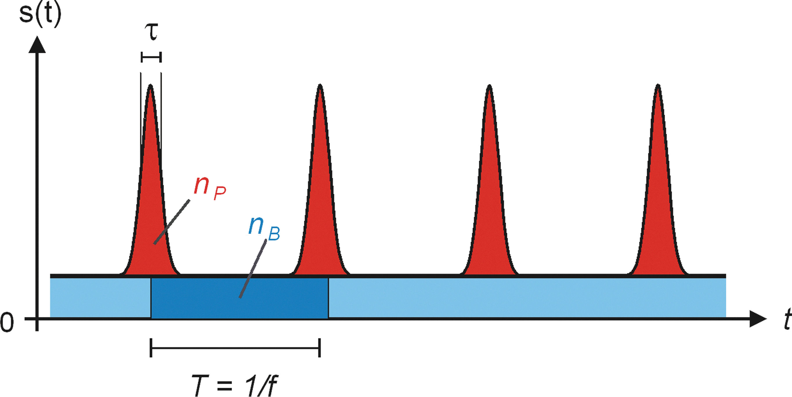
Assumed optical input signal consisting of repetitive pulses with low duty cycle τ/T, carrying n _P photons each (peaks, in red), and of background radiation (horizontal pedestal, light blue) with n _B background photons per period T (dark blue). Color images available online at www.liebertonline.com/ast

3. Signal Detection Equipment

3.1. Basic layout

The main purpose of our detection equipment is to deliver a digital electrical pulse for (more or less) each incoming photon and to furnish each pulse with precise time-of-arrival information (see Fig. 2). Serving as an optical receive antenna, a telescope is directed to the star system under investigation or, alternatively, just scanning the sky. At its focal plane, the radiation received is coupled into a multimode fiber3, possibly spectrally filtered by an optical band pass4, and fed into one or more single-photon avalanche detectors (SPADs), operated in the Geiger mode (Cova et al., 1996). In the case where several SPADs are employed, a fiber beam splitter will equally distribute the optical power among the SPADs. When the detector is struck by a photon, it will produce a narrow pulse at its electrical output with a steep rising edge that indicates the time of detection; however, only with a probability corresponding to its detection efficiency η. The SPAD thus acts as a trigger device, with the photon being the trigger and a digital electrical pulse constituting the output. In this work, we will refer to the latter as an “event.”

FIG. 2.

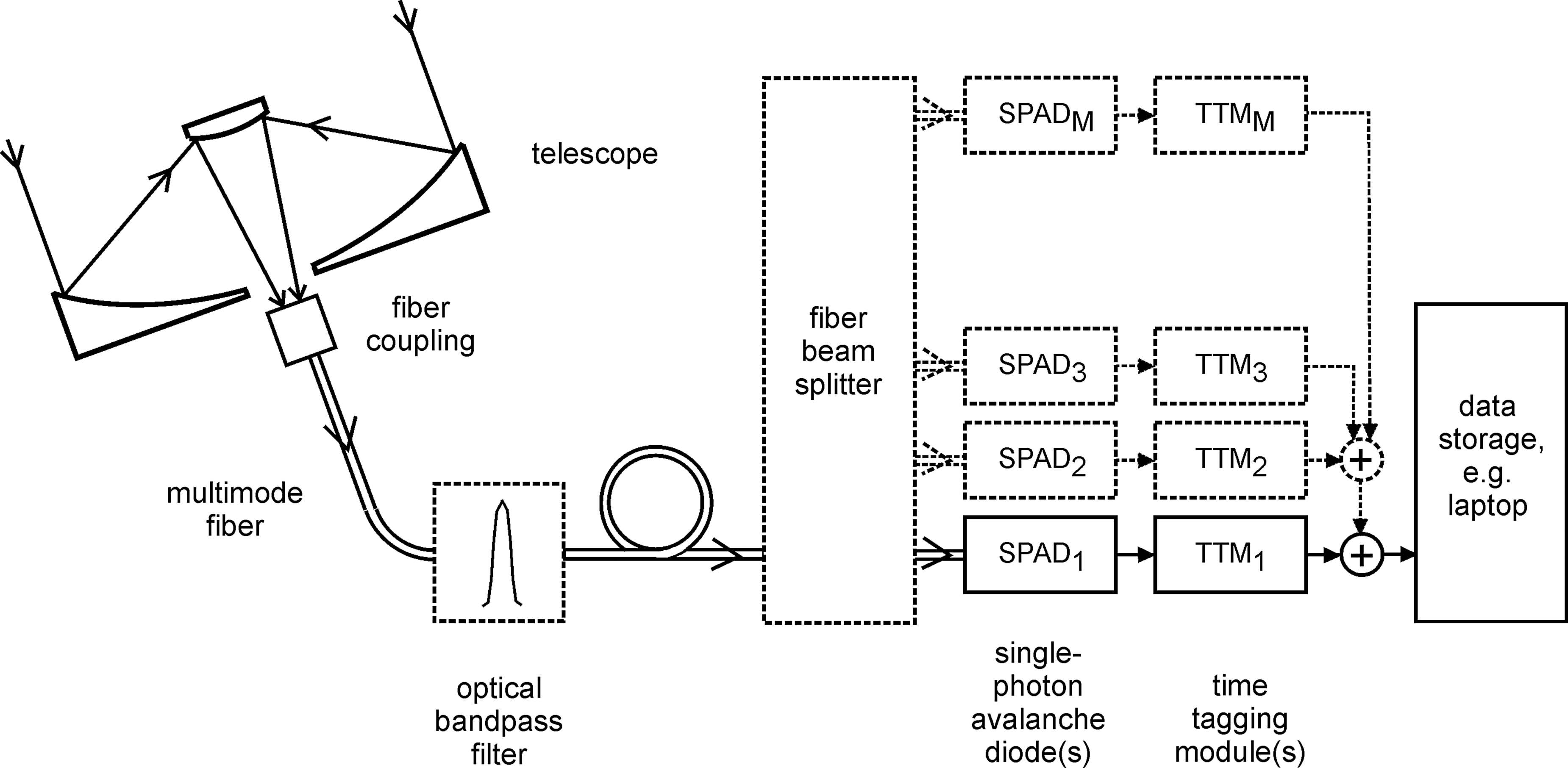
Block diagram of the signal detection equipment designed to record the precise time of arrival of photons originated by extraterrestrial intelligence. The subscripts 1 to M identify the individual channels in case of employing more than one detection channel.

In the subsequent module, each electrical pulse is time tagged at its rising edge with sub-nanosecond resolution and also marked with a channel indicator, which allows us to analyze each channel signal independently. Time tagging of all modules is properly synchronized. Lastly, the data is stored in a computer. Each entry consists of the relative arrival time of the detected photon (t_i ), see Fig. 3, as well as of the channel number. A digital time sequence resulting from a single channel is sketched in Fig. 3. The red (full) events are thought to originate from the periodic optical signal (frequency f, period T=1/f). As indicated, the recorded extraterrestrial events will not necessarily occur periodically. This may be due to time-varying absorption along the line of sight from the exoplanet or to turbulent atmosphere. In the case of low average optical input power per pulse, this may just be the manifestation of the Poisson distribution of photons. The random blue (dashed) events are caused by background photons and detector imperfections. They constitute the noise in the search for the periodic signal.

FIG. 3.

Sketch of digital time sequence of events occurring at time instants t_i . The red (full) events are thought to originate from the periodic optical extraterrestrial signal (frequency f, period T=1/f). The random blue (dashed) events are generated by background photons and detector imperfections. Color images available online at www.liebertonline.com/ast

3.2. Hardware

For the laboratory tests described in Section 5, we implemented the detection system without an optical band pass filter, as the involved sources were narrowband lasers.

Single-photon detection was performed with a commercially available four-channel device [“single-photon counting module array” type SPCM-AQ4C from PerkinElmer (2005)]. The fiber-coupled detector elements are silicon avalanche photodiodes biased above breakdown voltage, sensitive in the spectral region from 400 to 1060 nm. At a wavelength of 850 nm, the quantum efficiency is some 40%. After a photon has triggered an event, the detector is insensitive to incident light for a period of time called dead time. We could verify the dead time to amount close to the specified 50 ns, with slight variation among the four detector elements. When drawing Fig. 3, we assumed that the detector dead times are clearly smaller than T, the period of the extraterrestrial signal. This restriction, however, should be irrelevant in practice: Interstellar signaling asks for very high energy per optical pulse, most likely achievable only by a trade-off with low-repetition frequency, that is, a relatively large period T. The detector noise of the thermoelectrically cooled photodiodes is specified to be less than 500 counts s⁻¹. However, for the four diodes in the module available we measured dark count rates between 1500 and 2500 counts s⁻¹. The manufacturer further speaks of an “afterpulsing probability” of 0.5%. Investigating the diodes at hand revealed that a dead time was followed by an internally generated event with a probability of 1.4%. The electrical output pulses of the four channels are 25 ns wide TTL5 pulses.

The four time-tagging modules (TTMs) are homemade electronics (AIT, 2012) that provide the numerically encoded relative instant of time for each event. They were developed around the TDC GPX time to digital converter of Acam (2012). With proper supporting electronics, a stability of the time-tagging device similar to that of an atomic clock can be achieved; the temperature-stabilized internal quartz may be locked to a precise atomic clock or controlled by a 1 Hz GPS signal. However, our measurements were done in a free-running mode, which may result in a highly constant drift of less than 100 ns s⁻¹. For our typical measurement duration, this drift did not affect our data analysis. The detection of each event is measured with a timing resolution of 0.1 ns.

4. Data Processing Strategy

Our assumption was that any extraterrestrial intelligence could have transmitted a laser signal consisting of periodic pulses. Hence, we had to cope with the task of finding an originally periodic signal with unknown repetition frequency f=1/T within a seemingly random data sequence. In other words, we were looking for the red (full) lines of Fig. 3, which have a mutual distance of T or multiples thereof.

To this end, we first calculate the time differences t_i −t_j between the detected events (denoted t_i,j from now on) and display them in a histogram, that is, essentially the density function of the time differences. The histogram will show the number of occurrences (customarily denoted “frequency” and designated F in the following, but to be distinguished from the pulse repetition frequency f) within bins of time span bw versus t_i,j . Any periodic signal would manifest itself as distinct peaks around \documentclass{aastex}\usepackage{amsbsy}\usepackage{amsfonts}\usepackage{amssymb}\usepackage{bm}\usepackage{mathrsfs}\usepackage{pifont}\usepackage{stmaryrd}\usepackage{textcomp}\usepackage{portland, xspace}\usepackage{amsmath, amsxtra}\pagestyle{empty}\DeclareMathSizes{10}{9}{7}{6}\begin{document}$$t_{ij} = q {\cdot} T (q = 1 , 2 , 3 , \ldots)$$ \end{document} 6. For the considerations to follow, we make the reasonable assumption that the optical input pulses have a width smaller than the detector dead time.

4.1. Concepts

(a) Maximum utilization of the information contained in the data sequence would be made if all possible time differences t_i,j were used for generating the histogram, that is, when taking all possible combinations of t_i,j with \documentclass{aastex}\usepackage{amsbsy}\usepackage{amsfonts}\usepackage{amssymb}\usepackage{bm}\usepackage{mathrsfs}\usepackage{pifont}\usepackage{stmaryrd}\usepackage{textcomp}\usepackage{portland, xspace}\usepackage{amsmath, amsxtra}\pagestyle{empty}\DeclareMathSizes{10}{9}{7}{6}\begin{document} \begin{align*}j = 1 , 2 , \ldots , N - 1 \ {\rm and} \ i = j + 1 , j + 2 , \ldots , N \tag{1}\end{align*} \end{document}

where N denotes the last event (see Fig. 3). The total number of time differences then amounts to \documentclass{aastex}\usepackage{amsbsy}\usepackage{amsfonts}\usepackage{amssymb}\usepackage{bm}\usepackage{mathrsfs}\usepackage{pifont}\usepackage{stmaryrd}\usepackage{textcomp}\usepackage{portland, xspace}\usepackage{amsmath, amsxtra}\pagestyle{empty}\DeclareMathSizes{10}{9}{7}{6}\begin{document} \begin{align*}Y_N = \frac {N^2 - N} {2} \tag {2} \end{align*} \end{document}

In case of a data sequence consisting of, for example, N=50,000 events, the compilation of the histogram would ask for handling Y_N ≈1.25 billion data. Displaying all events in a histogram requires its (horizontal) t_i,j axis to cover a time interval equal to the total sequence measurement time t_N, ₁. The number of bins, B, to display along this axis is given by the quotient of t_N, ₁ and the bin width bw. It could become an impractically large number if t_N, ₁ were on the order of a second and bw would be kept as small as a few nanoseconds.

(b) Another extreme would be to utilize only the next consecutive event, that is, a restriction to all combinations of t_i,j with \documentclass{aastex}\usepackage{amsbsy}\usepackage{amsfonts}\usepackage{amssymb}\usepackage{bm}\usepackage{mathrsfs}\usepackage{pifont}\usepackage{stmaryrd}\usepackage{textcomp}\usepackage{portland, xspace}\usepackage{amsmath, amsxtra}\pagestyle{empty}\DeclareMathSizes{10}{9}{7}{6}\begin{document} \begin{align*}j = 1 , 2 , \ldots , N - 1 \ {\rm and} \ i = j + 1 \tag{3}\end{align*} \end{document}

Then the number of time differences to be handled is only \documentclass{aastex}\usepackage{amsbsy}\usepackage{amsfonts}\usepackage{amssymb}\usepackage{bm}\usepackage{mathrsfs}\usepackage{pifont}\usepackage{stmaryrd}\usepackage{textcomp}\usepackage{portland, xspace}\usepackage{amsmath, amsxtra}\pagestyle{empty}\DeclareMathSizes{10}{9}{7}{6}\begin{document} \begin{align*}Y_1 = N - 1 \tag{4}\end{align*} \end{document}

The horizontal axis of the histogram would cover a time given by the maximum time difference between consecutive events, max[t_j+ _1,j]. The histogram thus could not reveal signals with a period T>max[t_j+ _1,j]. Further, sequences with even modest numbers of background events would be difficult to detect.

(c) A third, attractive alternative is to restrict the time differences utilized by considering only a limited number, D, of consecutive events (D<N), that is, to use all possible combinations of \documentclass{aastex}\usepackage{amsbsy}\usepackage{amsfonts}\usepackage{amssymb}\usepackage{bm}\usepackage{mathrsfs}\usepackage{pifont}\usepackage{stmaryrd}\usepackage{textcomp}\usepackage{portland, xspace}\usepackage{amsmath, amsxtra}\pagestyle{empty}\DeclareMathSizes{10}{9}{7}{6}\begin{document} \begin{align*}j = 1 , 2 , \ldots , N - 1 \ {\rm and} \ i = j + 1 , j + 2 , \ldots , \min [j + D , N] \qquad\qquad\quad\quad\quad\quad (5) ^7\end{align*} \end{document}

The time differences defined by Eq. 5 are the elements in the top D diagonals of the matrix shown in Fig. 4, exemplary visualized by the blue (light and dark) squares for the case D=4. [All colored elements would be used in concept (a); only the light blue elements would be used in concept (b)].

FIG. 4.

Matrix representation of the time differences t_i,j used for concept (a)—all colored elements; for concept (b)—light blue elements in the top diagonal; and for concept (c)—light blue and dark blue elements. In this sketch, D=4. Color images available online at www.liebertonline.com/ast

For the third concept one has to handle \documentclass{aastex}\usepackage{amsbsy}\usepackage{amsfonts}\usepackage{amssymb}\usepackage{bm}\usepackage{mathrsfs}\usepackage{pifont}\usepackage{stmaryrd}\usepackage{textcomp}\usepackage{portland, xspace}\usepackage{amsmath, amsxtra}\pagestyle{empty}\DeclareMathSizes{10}{9}{7}{6}\begin{document} \begin{align*}Y_D = D {\cdot} N - \frac {D}{2} (D + 1) \tag {6} \end{align*} \end{document}

time differences. Clearly, the concepts (a) and (b) are special cases of concept (c) by choosing D=N − 1 and D=1, respectively. A proper choice of D will keep both Y_D and the number of bins B to be displayed reasonably low but at the same time utilize as much information as possible. A further advantage of concept (c) is that for D << N the extraterrestrial signal will show up in the histogram with peaks of more or less equal height all along the axis t_i,j . Of course, the challenge is to choose the to-be-analyzed length of the data sequence, that is, N or t_N, ₁, the bin width, and the value of D. (For some more details concerning these choices, see Subsection 6.1 and Appendix A).

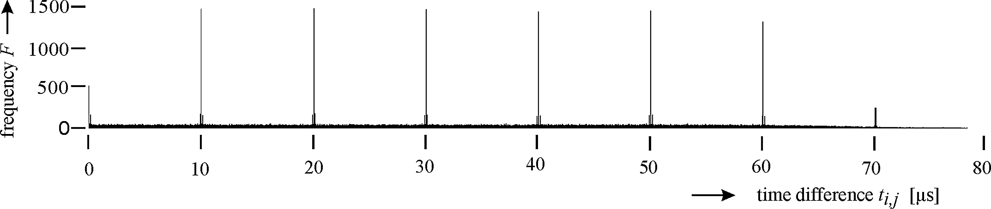
For the analysis of the measurements obtained during the laboratory tests (see Subsection 6.1), we decided to use the last concept, which we call “limited consecutive events method.” A typical resulting histogram looks like Fig. 5. For this specific case, we investigated a data sequence generated by a single channel (SPAD₁, TTM₁, see Fig. 2) in which the average number of photons per pulse was n _P=0.039 and the number of background photons per period was n _B=0.76. The sequence had a length of t_N, ₁=890 ms and contained N=28,300 events. The background events (indicated as the blue dashed lines in Fig. 3) are uncorrelated from each other and from signal events. They occurred with an average mutual time distance of 33 μs. In the histogram, they lead to the noise floor with fluctuations from bin to bin. The average distance between signal events (red lines in Fig. 3) was 664 μs. For the histogram shown in Fig. 5, we chose D=30, a bin width of bw=2.5 ns, and restricted the length of the horizontal axis to time differences t_i,j <200 μs, leading to B=80,000 bins displayed. The 20 peaks with a mutual distance of 10 μs clearly indicate the existence of periodic optical input pulses with a repetition frequency of f=100 kHz.

FIG. 5.

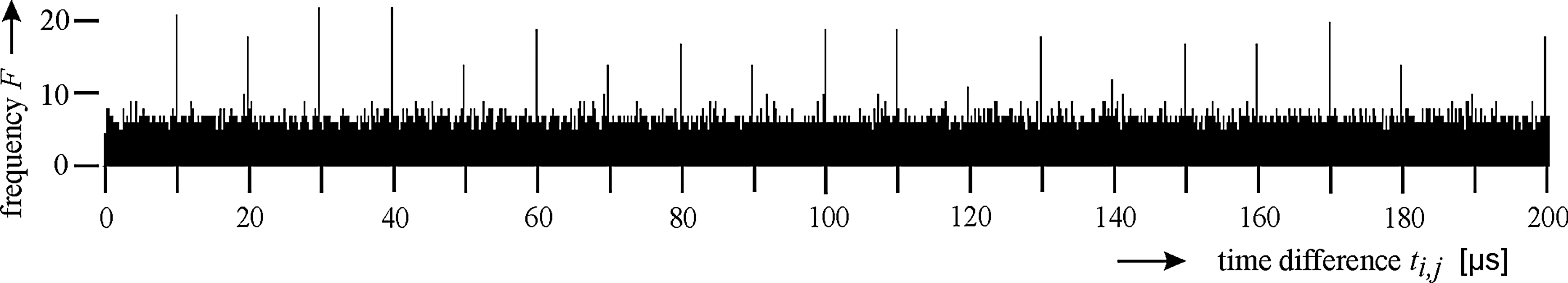
Example of a histogram obtained from a data string using only a single detection channel (n _P/n _B=0.05, N=28,300, t_N, ₁=890 ms, D=30, bw=2.5 ns).

4.2. Multiple detector system

In Fig. 2, we show a scheme in which several detection channels are used in parallel. It is worth noting the differences between this scheme and a single-channel scheme. Below we address the pros and cons of using multiple detectors.

(a) How does the number of events caused by “extraterrestrial photons” depend on the number, M, of single-photon detectors for a given number of average photons, n _P, per optical input pulse? For a single detector with a quantum efficiency η the probability p_M= ₁ for an event is \documentclass{aastex}\usepackage{amsbsy}\usepackage{amsfonts}\usepackage{amssymb}\usepackage{bm}\usepackage{mathrsfs}\usepackage{pifont}\usepackage{stmaryrd}\usepackage{textcomp}\usepackage{portland, xspace}\usepackage{amsmath, amsxtra}\pagestyle{empty}\DeclareMathSizes{10}{9}{7}{6}\begin{document} \begin{align*}p_{M = 1} = 1 - p_0 (n_{\rm P}{\cdot}\, \eta) \tag{7}\end{align*} \end{document}

where p ₀ denotes the probability that no event is generated. For Poisson-distributed photons we have \documentclass{aastex}\usepackage{amsbsy}\usepackage{amsfonts}\usepackage{amssymb}\usepackage{bm}\usepackage{mathrsfs}\usepackage{pifont}\usepackage{stmaryrd}\usepackage{textcomp}\usepackage{portland, xspace}\usepackage{amsmath, amsxtra}\pagestyle{empty}\DeclareMathSizes{10}{9}{7}{6}\begin{document} \begin{align*}p_0 (n_{\rm P} {\cdot}\, \eta) = \exp (- n_{\rm P} {\cdot}\, \eta) \tag{8}\end{align*} \end{document}

In case of M detectors and an equal split of the incoming photons among them, the events generated in each channel will be given by \documentclass{aastex}\usepackage{amsbsy}\usepackage{amsfonts}\usepackage{amssymb}\usepackage{bm}\usepackage{mathrsfs}\usepackage{pifont}\usepackage{stmaryrd}\usepackage{textcomp}\usepackage{portland, xspace}\usepackage{amsmath, amsxtra}\pagestyle{empty}\DeclareMathSizes{10}{9}{7}{6}\begin{document} \begin{align*}p_M = 1 - p_0 (n_{\rm P} \,{\cdot}\, \eta / M) \tag{9}\end{align*} \end{document}

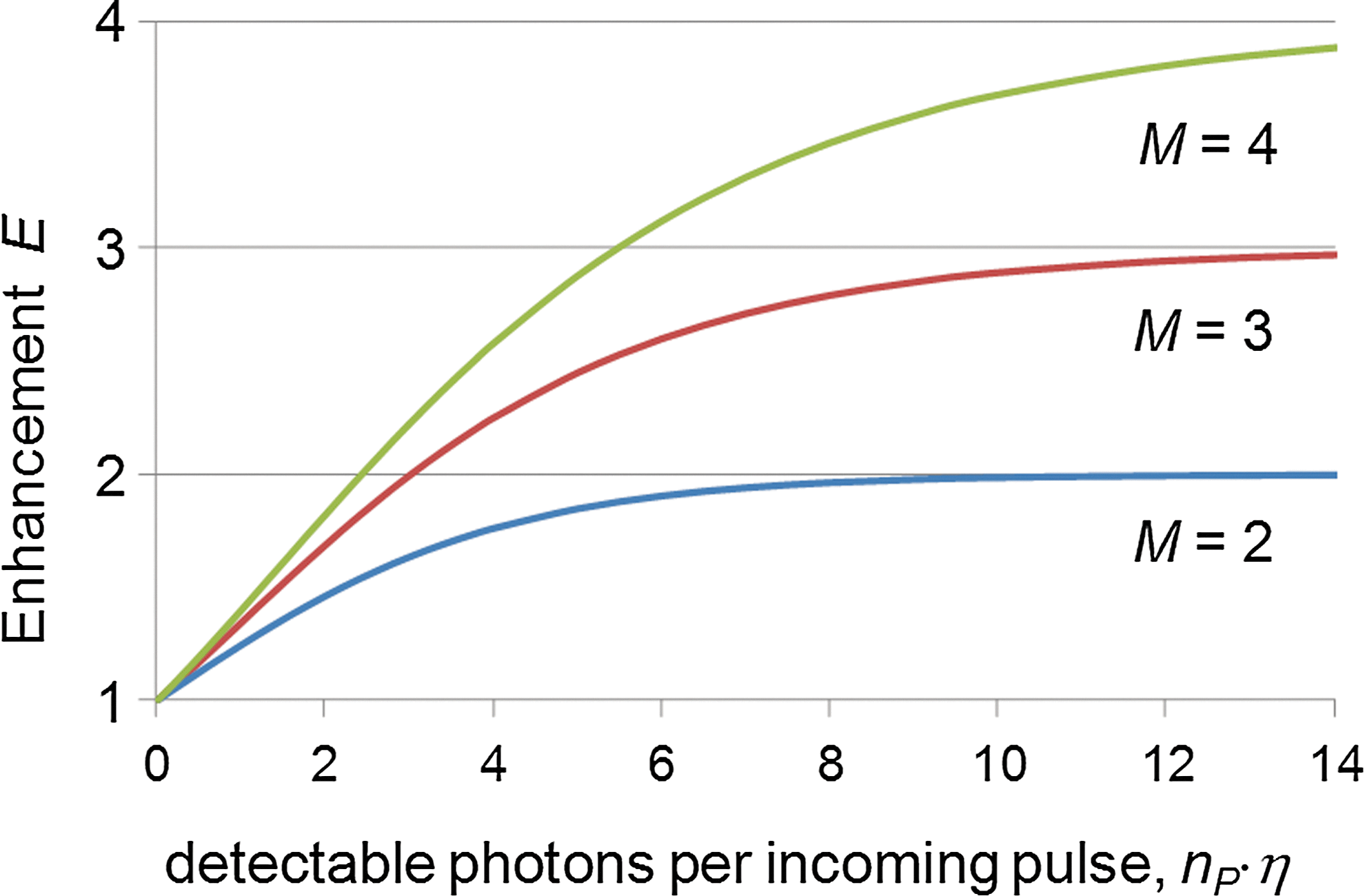
Figure 6 shows the enhancement E of the number of extraterrestrial events by using M channels when compared to the case of a single channel versus n _P·η, \documentclass{aastex}\usepackage{amsbsy}\usepackage{amsfonts}\usepackage{amssymb}\usepackage{bm}\usepackage{mathrsfs}\usepackage{pifont}\usepackage{stmaryrd}\usepackage{textcomp}\usepackage{portland, xspace}\usepackage{amsmath, amsxtra}\pagestyle{empty}\DeclareMathSizes{10}{9}{7}{6}\begin{document} \begin{align*}E = M \,{\cdot}\, p_M / p_{M = 1} \tag{10}\end{align*} \end{document}

FIG. 6.

Enhancement factor E of extraterrestrial events for M single-photon detectors. Color images available online at www.liebertonline.com/ast

For low numbers of detectable photons, Eq. 10 becomes \documentclass{aastex}\usepackage{amsbsy}\usepackage{amsfonts}\usepackage{amssymb}\usepackage{bm}\usepackage{mathrsfs}\usepackage{pifont}\usepackage{stmaryrd}\usepackage{textcomp}\usepackage{portland, xspace}\usepackage{amsmath, amsxtra}\pagestyle{empty}\DeclareMathSizes{10}{9}{7}{6}\begin{document} \begin{align*}E = 1 + (1 - 1 / M) \,{\cdot}\, n_{\rm P} \,{\cdot}\, \eta / 2 , (n_{\rm P} \,{\cdot}\, \eta < < 1) \tag{11}\end{align*} \end{document}

amounting to only E=1.1 (or 10%) for n _P·η=0.25 in case of four detectors (M=4). For a strong extraterrestrial pulse, each detector will produce an event; hence the enhancement factor approaches the number of detectors involved, M. Of course, losses caused by the beam splitter have to be considered as well. This effect would be fully felt at low photon numbers, while it could be more than compensated for by multiple detectors in case of strong input signal.

(b) How is the number of noise events (i.e., those caused by background photons, detector afterpulsing, and dark counts) influenced by the number of single-photon detectors? Certainly, the overall number of dark counts will be increased by a factor of ≈M. However, in the case of a relatively high background radiation of >2·10⁴ photons s⁻¹, as expected for a field measurement, this will cause little additional signal-to-noise deterioration if the dark counts are less than 2000 s⁻¹.

(c) The use of several detectors also offers a feature outside our intention of detecting periodic light pulses. If n _P·η is large enough to result in two events, even with low probability, the detectors of a two-detector system will produce them (almost) simultaneously. Such coincidences could be easily sought for by a simple search for double events defined by a mutual temporal distance t_j+ _1,j≤t _jitter, where a suitably chosen t _jitter allows for time jitter. This procedure would correspond to the coincidence method for detecting isolated pulses developed earlier (Wright et al., 2001; Howard et al., 2004).

When analyzing the experimental test sequences obtained in the laboratory (see Section 5), we observed a slight advantage for the system with four detectors (M=4) in the case of a low ratio of extraterrestrial photons to background photons.

Another aspect of using more than one detection channel is the possibility of simultaneous searching at different spectral bands by arranging spectral filters in front of each SPAD.

5. Laboratory Recordings

5.1. Setup

With no known extraterrestrial laser signal at hand, we had to test the detection equipment described in Section 3 in the laboratory. The source simulating the extraterrestrial signal consisted of a periodically pulsed diode laser operating at a wavelength of λ=850 nm. Background radiation was imitated by a second, continuously (cw) running diode laser emitting at the same wavelength (see Fig. 7). Both optical signals could be attenuated independently before being superimposed by a 1:1 fiber coupler. The following beam splitter diverted most of the power to another beam splitter, which fed both an optical power meter and a photodiode with a subsequent oscilloscope. These instruments allowed for verification of the shape and repetition frequency of the optical pulses and determination of the average power of the simulated extraterrestrial and background signals. The smaller portion of the combined signals passed another attenuator before being split into four roughly equal parts, each feeding a SPAD. Measuring the attenuation from the lower branch of the first 9:1 splitter to the power meter and to the four outputs of the 1:4 splitter permitted quantification of the number of background photons n _B per period T. When taking into account the pulse shape established with the oscilloscope, one can also estimate the number of photons per pulse, n _P. A typical pulse shape is displayed in Fig. 8. In this case, the pulse repetition frequency was f=100 kHz, corresponding to a period of T=10 μs.

FIG. 7.

Block diagram of laboratory setup when testing the detection equipment.

FIG. 8.

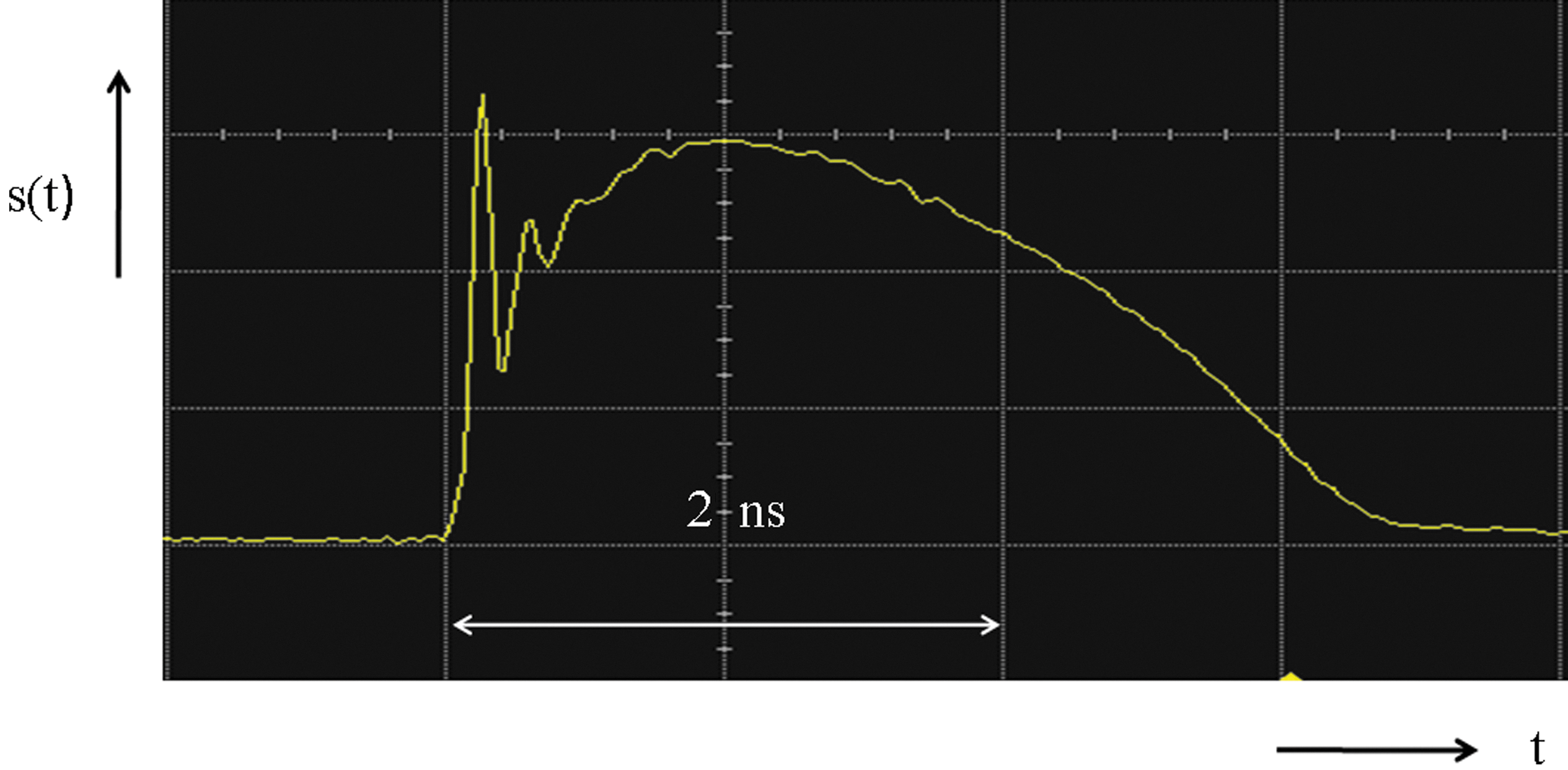
Shape s(t) of the optical input pulses generated by the laboratory laser source. The full-width half-maximum pulse width amounts to τ=2.45 ns. Color images available online at www.liebertonline.com/ast

The setup described thus can generate optical input signals as the one sketched in Fig. 1.

5.2. Parameters of data sequences recorded

With the setup described in Subsection 5.1, we recorded various data sequences, several with f=100 kHz and one with f=10 kHz. The (average) number of photons per pulse at the input of the 1:4 fiber splitter was in the range 0.12<n _P≤30. The number of background photons, n _B, per period 1/f was varied between nominally zero and n _B=6 by increasing the output power of the cw laser diode (see Fig. 7). (Note: even at n _B equal to zero, noise events are caused by detector dark counts and by “afterpulsing.”) The length of time we recorded one specific data sequence was on the order of 1 min. From this we typically used only a very small fraction (1 ms<t_N, ₁<1 s) for the analysis, with the number of events amounting up to N=30,000. Table 1 lists the parameters of those data sequences whose analyses and relevant histograms are to be presented in Section 6. The last column gives the ratio of photons per pulse n _P and background photons n _B per period T. It can serve as a measure of the input signal-to-noise ratio.

Table 1.

Input Parameters of the Data Sequences Analyzed in Section 6

Data sequence	f [kHz]	n _P	n _B	t _25,600,1 [ms]	n _P/n _B
DS-1	100	30	66	8.35	0.445
DS-2	100	2.3	74	8.45	0.032
DS-3	100	0.14	5.1	121	0.027
DS-4	10	0.12	2.0	3020	0.060

f=pulse repetition frequency; n _P=number of photons per pulse; n _B=background photons per period T; t _25,600,1=measurement time for N=25,600 events.

6. Analysis of Laboratory Data

6.1. Histograms

Using the concept put forward in Subsection 4.1(c), we constructed histograms showing the frequency F of time differences t_i,j for the data sequences DS-1 to DS-4. Beforehand, we had to make a choice for the histogram bin width bw, for the parameter D, that is, the number of consecutive events to be used, and lastly decide on the length of the histogram axis to be displayed.

The choice of bin width bw is driven by two main aspects: The best possible detectability of the periodic signal disrupted by the noise floor asks for a low bw (cf. square root term in Eq. A16). On the other hand, in a field measurement the detected extraterrestrial events will not be perfectly periodic but will have some time jitter caused by the transmitter, by time-varying propagation through space, and by jitter introduced by the detection equipment. These three effects determine a lower limit for bw (cf. term erf in Eqs. A16 and A10). For the laboratory recordings, it was relatively easy to discern that the simulated extraterrestrial events occurred with a time jitter with a standard deviation σ_e between 0.3 and 1.1 ns around each nominal pulse time instant q·T when a single SPAD was used. In the case of using all four SPADs, the jitter was found to be larger by a factor of about four. This effect could be traced back to a relative time delay of up to 4 ns between the four channels, introduced most likely by unequal lengths of optical and electrical cables. This misalignment could be corrected to a high degree ex post by applying a proper time correction for the events generated by three of the four channels. Altogether, a reasonable choice for the bin width could be 4σ_e (see Appendix A). This suggests a minimum bin width on the order of bw=3 ns for our recordings. When analyzing field measurements of unknown origin, the choice of bw is, of course, more delicate.

Another aspect concerning the histogram bin width is that a perfect periodicity of the detected pulses will be disturbed if the geometric distance between transmitter and receiver changes nonlinearly with time. This may be caused by the orbit of the exoplanet around its host star and that of Earth around the Sun. For reasonably short lengths of data sequences, t_N, ₁, a sufficiently high repetition frequency f, and an Earth-like exoplanet these effects will be negligible. However, the extraterrestrial intelligence could compensate for these effects by slightly adjusting the times at which the pulses are transmitted, and Earth-based scientists could compensate for them via subsequent adjustment of the time of pulse arrival.

The choice of D has two aspects: A large value will increase the number of time differences utilized and thus the information content of the histogram. In particular, it increases q, the number of peaks in the histograms (see Appendix A). In the examples shown below, D varies between 10 and 300. For the number of events taken (8400<N<25,600), D is small enough to keep the number of time differences Y_D to be handled (see Eq. 6) reasonably low.

A guideline for a choice for the maximum length of the histogram axis is also contained in Appendix A.

Table 2 presents the parameters chosen when analyzing our laboratory recordings, including the number of pulse periods P within the measurement time t_N, ₁. One further finds the number of events due to the periodic pulses and that of noise events, N _e and N _b, respectively, as obtained by an in-depth analysis. Their accuracy is estimated to be 3%.8 To obtain the histograms of Figs. 9 –12, we employed the statistics software R (R Core Development Team, 2012). On a PC, the computation time for generating a typical histogram was a few seconds, at most.

FIG. 9.

Histogram obtained for data sequence DS-1. For the parameters, see Table 2.

FIG. 10.

Histogram obtained for data sequence DS-2. For the parameters, see Table 2.

FIG. 11.

Histogram obtained for data sequence DS-3. For the parameters, see Table 2.

FIG. 12.

Histogram obtained for data sequence DS-4. For the parameters, see Table 2.

Table 2.

Characteristics of the Data Strings Analyzed and Histogram Parameters Used for Establishing the Histograms

Data sequence	t _N,1 [ms]	P	D	bw [ns]	N _e	N _b	p _e=N _e/(N _e+N _b)
DS-1	1.0	100	200	3	385	2,636	0.127
DS-2	8.45	845	300	2.5	705	24,890	0.028
DS-3	115	11,500	74	3	653	23,690	0.027
DS-4	1,000	10,000	10	12	539	7,905	0.064

In all cases, four detection channels were used.

t_N,1 =measurement time; P=number of periods within measurement time; D=number of consecutive events used; bw=bin width; N _e=number of pulse events recorded; N _b=number of noise events recorded; p _e=fraction of pulse events.

The histogram of Fig. 9 represents the case of a received optical pulse that is very strong; for 86% of the periods, all four detectors produced a pulse event. Approximately n _P=30 photons per pulse entered the 1:4 beam splitter (see Subsection 6.2). The input signal-to-noise ratio was n _P/n _B=0.445. The peaks observed would raise no doubt about an artificial input signal with a repetition frequency of 100 kHz, though the temporal length of the data string used for establishing the histogram was just 1 ms.

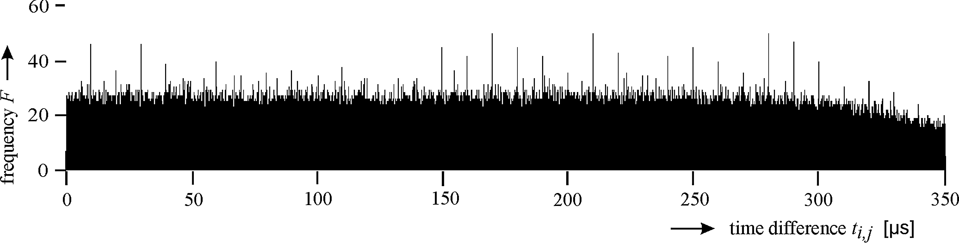
For Fig. 10, the average number of photons per pulse was only n _P=2.3, and the ratio of extraterrestrial photons to background photons is just n _P/n _B=0.032. Still, the 9+peaks (nine due to the choice of D, see Appendix A) at multiples of 10 μs are a clear indication of a periodic signal at f=100 kHz. The data string used here lasted 8.5 ms. As in Fig. 9, the length of the histogram x axis was chosen to slightly exceed the calculated value t_i,j, _max (compare Eq. A2).

The data sequence that led to the histogram of Fig. 11 produced pulse events only for 5.6% of the optical input pulses. The number of background photons per period T was n _B=5.1. Although the frequency of the peaks shows quite some variation with q, the existence of a periodic signal in the 115 ms long input string is evident.

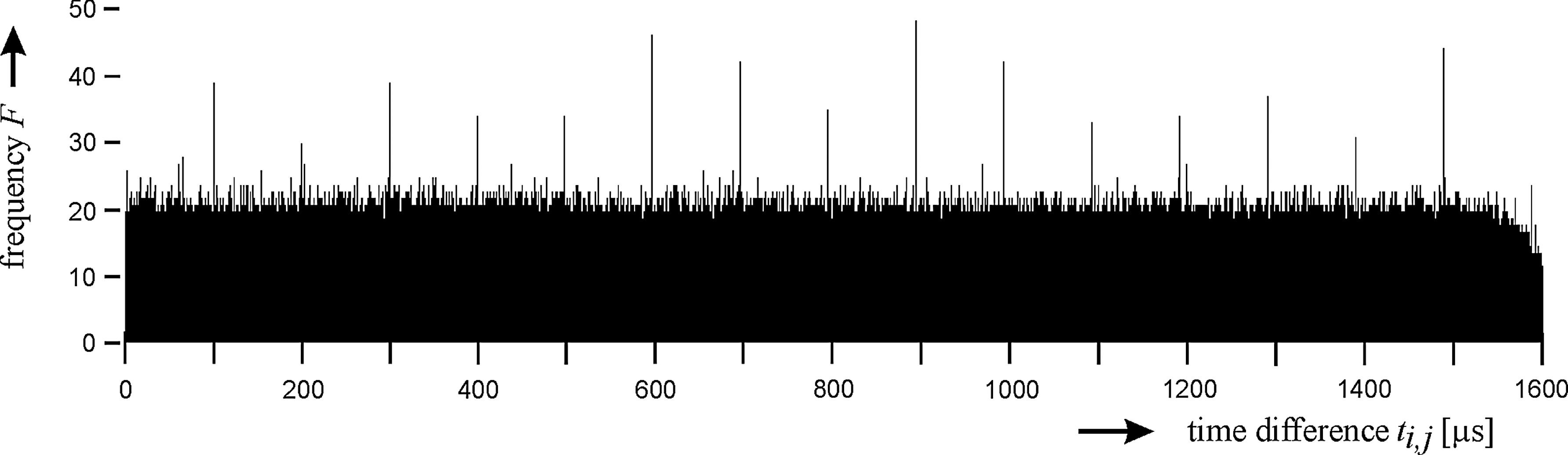
While the first three histograms resulted from signals pulsed at a rate of 100 kHz, the data sequence leading to Fig. 12 was pulsed at only 10 kHz. Still, if one spends sufficient time for recording the input signal, strong evidence can be obtained by properly chosen histogram parameters. For the histogram presented, a data string of 1 s length was used, with an input signal-to-noise ratio of n _P/n _B=0.06.

Figure 10 reveals the general form of the histograms in case of N >> D >> 1 quite clearly; a noisy floor caused by background events extends up to a value of about t_i,j, _max with constant mean value. This behavior eases the (computerized) detection of the peaks caused by the periodic signal. From here on, the noise level gently approaches the horizontal axis. (For the extreme cases D=N − 1 and D=1 [cf. Subsections 4.1(a) and 4.1(b)] the noise floor decreases monotonically from t_i,j =0 to t_i,j, _max.)

The above four examples demonstrate that the method proposed will provide excellent detectability of faint periodic pulses for a wide range of parameters of the optical input signal, at least when inspected by the human eye. In general, we require that the peaks at t_i,j =q·T stand out of the randomly varying floor. This can be formulated mathematically by requiring F _e>4σ_Fb, where F _e stands for the frequency of events caused by signal pulses and σ_Fb stands for the standard deviation of the frequency of the noise events F _b (see Appendix A). We have already begun to implement signal processing algorithms that will automatically recognize the equidistant peaks of unknown (!) periodicity T. So far the results are promising, not only for easy cases like those shown in Figs. 9, 10, and 12 but also in the case of Fig. 11 and for the histogram derived from a realistic scenario (see Section 7, Fig. 13).

FIG. 13.

Histogram obtained for the computer-generated data sequence simulating a periodic input signal (repetition frequency f=10 kHz) of duration t_N, ₁=24 ms, emitted from an exoplanet at a distance of 500 ly. The assumed received signal strength is n _R=1 photon per period; the background photon rate caused by the host star is r _B=1.54·10⁶ s⁻¹.

6.2. Number of incident pulse photons n_P

As mentioned above, an in-depth analysis of the data sequences allowed for classification, with high confidence, of each event with regard to whether it was caused by one of the periodic optical input pulses or simply a noise event, that is, due to background or “afterpulsing.” We were also able to discern which channel (consisting of a SPAD and a TTM) generated every single extraterrestrial event. By analyzing the events of just one channel, one may infer n _P, the number of photons per pulse incident on the entire detection equipment consisting of, for example, four channels, in the following way:

• Take the sequence of events from just one of the channels,

• find the number of events N _e due to laser pulses,

• with the known number of signal periods P in a measurement sequence calculate p_M , the probability of having detected a photon via \documentclass{aastex}\usepackage{amsbsy}\usepackage{amsfonts}\usepackage{amssymb}\usepackage{bm}\usepackage{mathrsfs}\usepackage{pifont}\usepackage{stmaryrd}\usepackage{textcomp}\usepackage{portland, xspace}\usepackage{amsmath, amsxtra}\pagestyle{empty}\DeclareMathSizes{10}{9}{7}{6}\begin{document} \begin{align*}p_M = N_e / P \tag{12}\end{align*} \end{document}

• combine Eqs. 8 and 9, which characterize the detection process of Poisson-distributed photons, yielding \documentclass{aastex}\usepackage{amsbsy}\usepackage{amsfonts}\usepackage{amssymb}\usepackage{bm}\usepackage{mathrsfs}\usepackage{pifont}\usepackage{stmaryrd}\usepackage{textcomp}\usepackage{portland, xspace}\usepackage{amsmath, amsxtra}\pagestyle{empty}\DeclareMathSizes{10}{9}{7}{6}\begin{document} \begin{align*}p_{M} = 1 - \exp (- n_{\rm P} \,{\cdot}\, \eta / M) \tag{13}\end{align*} \end{document}

• from which n _P, the number of photons per pulse is found for known SPAD efficiency η and number of channels M (η=0.4 and M=4 in our case). If the splitting ratio of the fiber beam splitter employed differs from 1/M, a corresponding weighting factor characterizing the channel used has to be applied.

Table 3 lists the values of p_M and n _P for the sequences reported in Subsection 6.1. (The numbers for n _P have already been presented in Table 1.)

Table 3.

Number of Photons per Pulse n _P for the Data Sequences under Consideration as Obtained by Determining the Probability p _M of Detecting One Photon at the Channel with Single-Photon Avalanche Diode SPAD ₁

Data sequence	p_M	n _P
DS-1	0.9665	30
DS-2	0.228	2.3
DS-3	0.0155	0.14
DS-4	0.0152	0.12

7. Concept Test of a Fictitious Scenario

Investigation of the laboratory data with the concept put forward in Subsection 4.1(c) yielded the promising results presented in Subsection 6.1. Therefore, as a next step, we tested our method on a fictitious but realistic scenario.

We simulate a scenario where an extraterrestrial pulsed laser signal with repetition frequency f=10 kHz and wavelength λ=850 nm is transmitted from an exoplanet that orbits a 500 ly distant G2V-type star. The diameter of the diffraction-limited transmit telescope is D _T=10 m, and the number of emitted photons per pulse is such that, on Earth, a receiving telescope with diameter D _R=1.7 m would collect—on average—just n _P=1 photon per pulse. It can be shown that this requires a transmit pulse energy of 4.2·10⁴ J, corresponding to 1.8·10²³ photons if a space transmission loss of 50% is assumed.

Background photons at the receiver will be dominated by host star radiation. In this respect, we assume a stellar surface temperature of 5900 K and a stellar diameter of 1.4·10⁹ m, which equals one Sun diameter. Then the rate of background photons received can be calculated to be r _B=1.54·10⁶ s⁻¹, assuming a receiver bandwidth of Δλ=290 nm centered around λ=850 nm9.

For the above input signal, we then computer-generated a data string that simulates the event sequence to be expected at the output of TTM₁ (see Fig. 2). The detector was modeled as a single SPAD (i.e., M=1) with a quantum efficiency of η=0.4, assumed to be constant over the entire bandwidth Δλ. To generate the event sequence, we had to determine

• the average time difference between consecutive events, t_i,j, _av,

• the number of background events, N _b,

• the number of pulse events, N _e, and

• the “measurement” time, t_N, ₁.

First, we chose the length of the data string, N=N _b+N _e, to be N=15,000. For N _b >> N _e, t_i,j, _av follows from the background photon rate and the quantum efficiency as \documentclass{aastex}\usepackage{amsbsy}\usepackage{amsfonts}\usepackage{amssymb}\usepackage{bm}\usepackage{mathrsfs}\usepackage{pifont}\usepackage{stmaryrd}\usepackage{textcomp}\usepackage{portland, xspace}\usepackage{amsmath, amsxtra}\pagestyle{empty}\DeclareMathSizes{10}{9}{7}{6}\begin{document} \begin{align*}t_ {i , j , {\rm av}} \approx \frac {1} {r_ {\rm B} {{\cdot} \,} \eta} = 1.62 \ \mu {\rm s} \tag {14} \end{align*} \end{document}

while the “measurement” time is given by \documentclass{aastex}\usepackage{amsbsy}\usepackage{amsfonts}\usepackage{amssymb}\usepackage{bm}\usepackage{mathrsfs}\usepackage{pifont}\usepackage{stmaryrd}\usepackage{textcomp}\usepackage{portland, xspace}\usepackage{amsmath, amsxtra}\pagestyle{empty}\DeclareMathSizes{10}{9}{7}{6}\begin{document} \begin{align*}t_{N , 1} \approx N \,{\cdot}\, t_{i , j , {\rm av}} = 24.4 \ {\rm ms} \tag{15}\end{align*} \end{document}

(compare Appendix A, Eq. A1). The number of full periods within the data string, P, and the number of pulse events, N _e, are \documentclass{aastex}\usepackage{amsbsy}\usepackage{amsfonts}\usepackage{amssymb}\usepackage{bm}\usepackage{mathrsfs}\usepackage{pifont}\usepackage{stmaryrd}\usepackage{textcomp}\usepackage{portland, xspace}\usepackage{amsmath, amsxtra}\pagestyle{empty}\DeclareMathSizes{10}{9}{7}{6}\begin{document} \begin{align*}P = \left] \frac {t_ {N , 1}} {T} \right[= 243 \tag {16} \end{align*} \end{document}

where the symbol ][ stands for rounding down to the next integer (recall that T=1/f), and \documentclass{aastex}\usepackage{amsbsy}\usepackage{amsfonts}\usepackage{amssymb}\usepackage{bm}\usepackage{mathrsfs}\usepackage{pifont}\usepackage{stmaryrd}\usepackage{textcomp}\usepackage{portland, xspace}\usepackage{amsmath, amsxtra}\pagestyle{empty}\DeclareMathSizes{10}{9}{7}{6}\begin{document} \begin{align*}N_e = P {\,{\cdot}\,} p_{M = 1} \tag{17}\end{align*} \end{document}

The term p_M= ₁ in Eq. 17 was already introduced in Subsection 4.2, Eq. 7. It is the probability for the generation of one event (per period) when employing only one single-photon detector with a quantum efficiency η. For Poisson-distributed photons, Eqs. 8 and 9 yield \documentclass{aastex}\usepackage{amsbsy}\usepackage{amsfonts}\usepackage{amssymb}\usepackage{bm}\usepackage{mathrsfs}\usepackage{pifont}\usepackage{stmaryrd}\usepackage{textcomp}\usepackage{portland, xspace}\usepackage{amsmath, amsxtra}\pagestyle{empty}\DeclareMathSizes{10}{9}{7}{6}\begin{document} \begin{align*}p_{M = 1}= 1- \exp ( - n_{\rm P} {{\cdot}\,}\eta ) \tag{18}\end{align*} \end{document}

For n _P=1 and η=0.4, we obtain \documentclass{aastex}\usepackage{amsbsy}\usepackage{amsfonts}\usepackage{amssymb}\usepackage{bm}\usepackage{mathrsfs}\usepackage{pifont}\usepackage{stmaryrd}\usepackage{textcomp}\usepackage{portland, xspace}\usepackage{amsmath, amsxtra}\pagestyle{empty}\DeclareMathSizes{10}{9}{7}{6}\begin{document} \begin{align*}N_e = 80 \tag{19}\end{align*} \end{document}

which leads to N _b=14,920 and p _e=N _e/N=0.0053 for the fraction of pulse events.

The time instants of the background events were generated by a random sequence; the time instants for the pulse events were obtained by a random choice among all possible time instants \documentclass{aastex}\usepackage{amsbsy}\usepackage{amsfonts}\usepackage{amssymb}\usepackage{bm}\usepackage{mathrsfs}\usepackage{pifont}\usepackage{stmaryrd}\usepackage{textcomp}\usepackage{portland, xspace}\usepackage{amsmath, amsxtra}\pagestyle{empty}\DeclareMathSizes{10}{9}{7}{6}\begin{document}$$m \,{\cdot}\, T \ (m = 1 , 2 , \ldots , N_e)$$ \end{document} with probability prob=N _e /P=0.33. In both cases, the time resolution was 0.1 ns.

From the so-generated data string, we calculated a histogram of the time differences, as exemplified in Subsection 6.1. This required a choice of consecutive events D and of the bin width bw. In particular, we decided for D=1000 and bw=1 ns. Figure 13 presents a histogram resulting from one realization. The more-or-less regular time difference of the dominant peaks in the histogram shows that there was a periodic signal embedded in the background noise, with period T=100 μs, corresponding to a laser pulse repetition frequency of f=10 kHz. Figure 14 details the area near the first peak. It uncovers the individual bins and evinces the values of the average noise frequency (F _b=9.2), its standard deviation (σ_Fb=3.0), and the average frequency caused just by the pulse events (F _e=26.9, in case of erf=1), as obtained by using Eqs. A14, A15, and A11.

FIG. 14.

Detail of Fig.13, showing the first peak.

8. Summary and Outlook

We assumed that extraterrestrial civilizations could have purposely transmitted optical radiation toward Earth to make us know of their existence. It is not unlikely that such civilizations would use periodic laser pulses with a repetition rate in the kilohertz to megahertz regime. Such a signal would not carry necessarily a message except that there is an extraterrestrial intelligence at a well-defined position in the Galaxy. However, its detection is entirely conceivable with present-day technology, even over distances of several hundred light-years.

We designed a technique that employs one or more single-photon avalanche diodes, which allows for the easy discovery of such optical pulse trains after a recording time of less than a second. Each event generated by a photodetector entails an electronic pulse that is time-stamped with a relative accuracy of 0.1 ns. A histogram of time differences between events reveals the periodic optical input pulses in the form of peaks separated by multiples of 1/f. For practical reasons, it is generally not advisable to process all available time differences when calculating the histogram. We have suggested the use of only a small percentage of consecutive events and presented an estimation framework of how this—and other parameters—influences the appearance of the histogram. Our results show that the use of more than one single-photon channel will not facilitate retrieving weak signals, that is, those with an average of only one photon per pulse or less. The prime criterion for detectability is the ratio of received photons per extraterrestrial pulse to the number of background photons per period 1/f. Increasing the receiving telescope diameter will not improve this ratio in the weak signal regime as long as dark counts are negligible. However, it would reduce the measurement time needed to achieve a certain signal-to-noise ratio. If, on the other hand, pulses with more than one photon per pulse are expected, increasing the number of detection channels would in general improve the ratio of extraterrestrial events to noise events.

With the technique described in this paper, the pulse width τ of the optical input signal (see Figs. 1 and 8) is of no concern. It may be anything from microseconds down to nominally zero, as is the case for a pulse containing just one photon. What is relevant for an unambiguous detection in a short measurement time is the energy (or number of photons) of the received pulses and the efficiency of their conversion into events. Therefore, it is advantageous to have detectors at hand with high quantum efficiency and to make every effort not to lose photons on their way from the telescope's primary mirror to the detector(s). Coupling the received radiation into an optical fiber right at the telescope's focal plane and using a fiber beam splitter in case of multichannel detection helps to achieve this goal. Besides a single fiber input coupling device, the concept requires no fine adjustment of bulk optical elements.

We tested the technique in the laboratory with lasers operating at 0.85 μm acting as extraterrestrial source (at f=100 kHz and f=10 kHz) and as background radiation. Even in the case of input signal-to-noise ratios as low as 3·10⁻², defined as the ratio of average received photons per pulse and background photons per period, the generated signal could be clearly detected.

Using synthetic data, we further demonstrated that the suggested technique would be sensitive enough to detect a faint, artificial, periodic laser signal traveling over a distance of 500 ly. In our specific example, receiving just a single photon from each of the laser pulses transmitted at a repetition frequency of 10 kHz would suffice to detect the artificial signal within an observation time of 24 ms. The energy of the pulses to be transmitted was calculated to be 42 kJ. As early as 2003, laser technology on Earth allowed for the generation of pulse energies of 21 kJ at λ=1.06 μm and 11.4 kJ at λ=0.53 μm (NIF, 2007), corresponding to 1.1·10²³ and 3.0·10²² photons. The repetition rate was stated as one shot every 5 h, however, with 192 such lasers now available. Recently, a laser system based on Ti:Sa lasers (λ=0.8 μm) operating at a rate of 1 Hz was commissioned (BELLA, 2012), though with a pulse energy of only 40 J.

So far the intention was to discover a beacon that is turned on and off periodically. From a strict communications point of view, the signal form we anticipated may be called quasi-periodic, as it is a finite section of a truly periodic—and thus everlasting—signal. In the examples presented, its duration, that is, the length of data strings, was 1 ms<t_N, ₁<1000 ms. Such a quasi-periodic signal could also be used as the basis for digital data transmission by assigning different cycle lengths T to different symbols. In the binary case, with T ₀, T ₁, however, the data rate R would be as low as 1/t_N, ₁, that is, on the order of 1<R<1000 bit s⁻¹. We have also begun to investigate the case where, instead of a highly periodic signal, pairs of laser pulses with constant time interval T _p are transmitted randomly (or at prescribed times). Such signaling shows up in the histogram as a single line at t_i,j =T _p.

The large number of data to be processed, stored, and analyzed presents a computational challenge. Presently, the bottleneck is not the number of data gathered but the generation of histograms, especially if the repetition rate of the incoming pulses is low. We are now developing improved algorithms that will allow handling pulse repetition frequencies down to the hertz regime. For analyzing very long data sequences, we have been working with a Visual Basic code using Excel-based graphics. Rather than having to cut out slices of the data stream and analyze them one by one, this software employs a moving analysis window that continuously looks for peaks in the histogram and assesses their relevance.

With the simple and extremely easy-to-implement equipment described above, we already have begun to make measurements with the 80 cm telescope of the Department of Astrophysics at the University of Vienna, targeting some recently detected exoplanets that supposedly lie in the habitable zone around their host star. A systematic survey is planned for the near future.

Our efforts constitute a further tiny step toward a possible answer to a very basic question of mankind: “Are we alone?” In particular, this work could provide clues as to whether a few hundred years ago an extraterrestrial intelligence directed at our solar system, at reasonably high repetition rates and in a well-collimated beam, laser pulses that consisted of some 10²³ photons each and operated at a wavelength for which we have efficient and fast single-photon detectors available.

Appendix A: Appearance of Histograms

After recording a data sequence of the form shown in Fig. 3, several parameters of the histogram must be selected so it can be computed and drawn. Below, we will derive equations that link various data sequence parameters like N, N _e, and t_N, ₁ with parameters that show up in the histogram. The parameters are the number of bins, B; the total length of the histogram abscissa, t_i,j, _max; the number of signal-related peaks, q _max; the bin width, bw; and the number of consecutive events, D (compare Fig. 4). In the following, we will mainly consider a detection system with only a single SPAD (M=1) and assume that the data sequence consists of N events (N >> 1), taken within a time period of t_N, ₁ (=t_N −t ₁). Considerations along this line also allow for discussion of the detectability of the unknown periodic signal, as it will emerge in the histogram.

To gain a rough insight into the relationship of the various parameters, we model the recorded events to be uniformly distributed10. Then the average time difference is \documentclass{aastex}\usepackage{amsbsy}\usepackage{amsfonts}\usepackage{amssymb}\usepackage{bm}\usepackage{mathrsfs}\usepackage{pifont}\usepackage{stmaryrd}\usepackage{textcomp}\usepackage{portland, xspace}\usepackage{amsmath, amsxtra}\pagestyle{empty}\DeclareMathSizes{10}{9}{7}{6}\begin{document} \begin{align*}t_ {i , j , {\rm av}} = \frac {t_ {N , 1}} {N} \tag {\rm A1} \end{align*} \end{document}

and, for D consecutive events chosen, the length of the histogram axis becomes \documentclass{aastex}\usepackage{amsbsy}\usepackage{amsfonts}\usepackage{amssymb}\usepackage{bm}\usepackage{mathrsfs}\usepackage{pifont}\usepackage{stmaryrd}\usepackage{textcomp}\usepackage{portland, xspace}\usepackage{amsmath, amsxtra}\pagestyle{empty}\DeclareMathSizes{10}{9}{7}{6}\begin{document} \begin{align*}t_{i , j , \max} \approx D \,{\cdot}\, t_{i , j , {\rm av}} \tag{{\rm A}2}\end{align*} \end{document}

while the number of bins is \documentclass{aastex}\usepackage{amsbsy}\usepackage{amsfonts}\usepackage{amssymb}\usepackage{bm}\usepackage{mathrsfs}\usepackage{pifont}\usepackage{stmaryrd}\usepackage{textcomp}\usepackage{portland, xspace}\usepackage{amsmath, amsxtra}\pagestyle{empty}\DeclareMathSizes{10}{9}{7}{6}\begin{document} \begin{align*}B = \frac {t_{l , j , \max}}{b \it w} \approx D \frac {t_{i , j , {\rm av}}}{b {w}} \tag{{\rm A}3}\end{align*} \end{document}

The bin width, bw, has still to be chosen. The number of peaks caused by the periodic events, q _max, that will appear in the histogram follows as \documentclass{aastex}\usepackage{amsbsy}\usepackage{amsfonts}\usepackage{amssymb}\usepackage{bm}\usepackage{mathrsfs}\usepackage{pifont}\usepackage{stmaryrd}\usepackage{textcomp}\usepackage{portland, xspace}\usepackage{amsmath, amsxtra}\pagestyle{empty}\DeclareMathSizes{10}{9}{7}{6}\begin{document} \begin{align*}q_ {\max} = \left] \frac {t_ {i , j , \max}} {T} \right[\approx \left] \frac {D \, {\cdot} \, t_ {N , 1}} {N \, {\cdot} \, T} \right[\approx \left] D \frac {t_ {i , j , {\rm av}}} {T} \right[\tag {{\rm A}4} \end{align*} \end{document}

where T is the period and the symbol ][ stands for rounding down to the next integer. Hence, to obtain at least the first peak (q=1), that is, the one at t_i,j =1·T, the condition \documentclass{aastex}\usepackage{amsbsy}\usepackage{amsfonts}\usepackage{amssymb}\usepackage{bm}\usepackage{mathrsfs}\usepackage{pifont}\usepackage{stmaryrd}\usepackage{textcomp}\usepackage{portland, xspace}\usepackage{amsmath, amsxtra}\pagestyle{empty}\DeclareMathSizes{10}{9}{7}{6}\begin{document} \begin{align*}D \geq \frac {N \, {\cdot} \, T} {t_ {N , 1}} \tag {{\rm A}5} \end{align*} \end{document}

has to be met.

Next, we determine the frequency F _e of differences between pulse events in the bins centered at \documentclass{aastex}\usepackage{amsbsy}\usepackage{amsfonts}\usepackage{amssymb}\usepackage{bm}\usepackage{mathrsfs}\usepackage{pifont}\usepackage{stmaryrd}\usepackage{textcomp}\usepackage{portland, xspace}\usepackage{amsmath, amsxtra}\pagestyle{empty}\DeclareMathSizes{10}{9}{7}{6}\begin{document}$$t_{i , j} = q \,{\cdot}\, T\, (q = 1 , 2 , 3 , \ldots q_{\max})$$ \end{document} . The number Y _e of time differences between pulse events within the upper D diagonals of Fig. 4 is approximated by \documentclass{aastex}\usepackage{amsbsy}\usepackage{amsfonts}\usepackage{amssymb}\usepackage{bm}\usepackage{mathrsfs}\usepackage{pifont}\usepackage{stmaryrd}\usepackage{textcomp}\usepackage{portland, xspace}\usepackage{amsmath, amsxtra}\pagestyle{empty}\DeclareMathSizes{10}{9}{7}{6}\begin{document} \begin{align*}Y_e = \frac {N_e^2 - N_e} {2} \frac {Y_D} {Y_N} \tag {{\rm A}6} \end{align*} \end{document}

where the first term gives all such time differences (N _e being the number of pulse events), and the second term, Y_D /Y_N , accounts for the fraction contained in the first D diagonals (cf. Eqs. 2 and 6). Here, we made the reasonable assumption that the noise events are randomly distributed between the pulse events. In the histogram, the average frequency of time differences between pulse events in each sufficiently wide bin at t_i,j =q·T follows as \documentclass{aastex}\usepackage{amsbsy}\usepackage{amsfonts}\usepackage{amssymb}\usepackage{bm}\usepackage{mathrsfs}\usepackage{pifont}\usepackage{stmaryrd}\usepackage{textcomp}\usepackage{portland, xspace}\usepackage{amsmath, amsxtra}\pagestyle{empty}\DeclareMathSizes{10}{9}{7}{6}\begin{document} \begin{align*}F_e^ {\prime} = \frac {Y_e} {q_ {\max}} = \frac {T} {2t_ {N , 1}} \frac {(p_e^2N^2 - p_eN) (2N - D - 1)} {N (N - 1)} \tag {{\rm A}7} \end{align*} \end{document}

In many practical cases, we have N >> 1, 2N >> D, p _e N=N _e >> 1, which simplifies Eq. A7 to \documentclass{aastex}\usepackage{amsbsy}\usepackage{amsfonts}\usepackage{amssymb}\usepackage{bm}\usepackage{mathrsfs}\usepackage{pifont}\usepackage{stmaryrd}\usepackage{textcomp}\usepackage{portland, xspace}\usepackage{amsmath, amsxtra}\pagestyle{empty}\DeclareMathSizes{10}{9}{7}{6}\begin{document} \begin{align*}F_e^ {\prime} = \frac {p_e^2ND} {q_ {\max}} \tag {{\rm A}8} \end{align*} \end{document}

Here, we have expressed the total number N _e of pulse events via their percentage p _e of all N recorded events, \documentclass{aastex}\usepackage{amsbsy}\usepackage{amsfonts}\usepackage{amssymb}\usepackage{bm}\usepackage{mathrsfs}\usepackage{pifont}\usepackage{stmaryrd}\usepackage{textcomp}\usepackage{portland, xspace}\usepackage{amsmath, amsxtra}\pagestyle{empty}\DeclareMathSizes{10}{9}{7}{6}\begin{document} \begin{align*}p_e = N_e / N \tag{{\rm A}9}\end{align*} \end{document}

In the case where the bin width is not much larger than the standard deviation σ of the probability density function of the jitter-caused distribution of the time differences between pulse events around q·T, some of these t_i,j would not show up in the proper bin, thus effectively reducing the value of \documentclass{aastex}\usepackage{amsbsy}\usepackage{amsfonts}\usepackage{amssymb}\usepackage{bm}\usepackage{mathrsfs}\usepackage{pifont}\usepackage{stmaryrd}\usepackage{textcomp}\usepackage{portland, xspace}\usepackage{amsmath, amsxtra}\pagestyle{empty}\DeclareMathSizes{10}{9}{7}{6}\begin{document}$$F_e^{\prime}$$ \end{document} . Assuming that the jitter may be modeled by a Gaussian process, this reduction factor is given by the error function of bw/(2σ_e). That is, by \documentclass{aastex}\usepackage{amsbsy}\usepackage{amsfonts}\usepackage{amssymb}\usepackage{bm}\usepackage{mathrsfs}\usepackage{pifont}\usepackage{stmaryrd}\usepackage{textcomp}\usepackage{portland, xspace}\usepackage{amsmath, amsxtra}\pagestyle{empty}\DeclareMathSizes{10}{9}{7}{6}\begin{document} \begin{align*}erf \left(\frac {b {w}} {2 \sigma_e} \right) = \frac {2} {\sqrt {2 \pi}} \int_0^ {\frac {b {w}} {2 \sigma_ {e}}} \,e^ {- \frac {z^2} {2}} {d} z \tag {{\rm A}10} \end{align*} \end{document}

The factor ½ in the argument of the error function stems from the fact that the bin width bw covers both sides to the central time instant t_i,j =q \documentclass{aastex}\usepackage{amsbsy}\usepackage{amsfonts}\usepackage{amssymb}\usepackage{bm}\usepackage{mathrsfs}\usepackage{pifont}\usepackage{stmaryrd}\usepackage{textcomp}\usepackage{portland, xspace}\usepackage{amsmath, amsxtra}\pagestyle{empty}\DeclareMathSizes{10}{9}{7}{6}\begin{document}$$\,{\cdot}\,$$ \end{document} T. As an example, a choice of bw=4σ_e would yield erf=0.95, that is, 5% of the pulse time differences would not show up in the expected bin. Hence, we modify \documentclass{aastex}\usepackage{amsbsy}\usepackage{amsfonts}\usepackage{amssymb}\usepackage{bm}\usepackage{mathrsfs}\usepackage{pifont}\usepackage{stmaryrd}\usepackage{textcomp}\usepackage{portland, xspace}\usepackage{amsmath, amsxtra}\pagestyle{empty}\DeclareMathSizes{10}{9}{7}{6}\begin{document}$$F_e^{\prime}$$ \end{document} in the form \documentclass{aastex}\usepackage{amsbsy}\usepackage{amsfonts}\usepackage{amssymb}\usepackage{bm}\usepackage{mathrsfs}\usepackage{pifont}\usepackage{stmaryrd}\usepackage{textcomp}\usepackage{portland, xspace}\usepackage{amsmath, amsxtra}\pagestyle{empty}\DeclareMathSizes{10}{9}{7}{6}\begin{document} \begin{align*}F_e = \frac {p_e^2ND} {q_ {\max}} \, {\cdot} \, erf \tag {{\rm A}11} \end{align*} \end{document}

where, for the sake of simplicity, we omit the argument of the error function from here on.

To determine the mean frequency F _b of time differences caused by background events per bin, we note that the total number Y _b of such time differences is \documentclass{aastex}\usepackage{amsbsy}\usepackage{amsfonts}\usepackage{amssymb}\usepackage{bm}\usepackage{mathrsfs}\usepackage{pifont}\usepackage{stmaryrd}\usepackage{textcomp}\usepackage{portland, xspace}\usepackage{amsmath, amsxtra}\pagestyle{empty}\DeclareMathSizes{10}{9}{7}{6}\begin{document} \begin{align*}Y_{\rm b} = Y_D - Y_e \tag{{\rm A}12}\end{align*} \end{document}

which, within the same approximation as just mentioned, simplifies to \documentclass{aastex}\usepackage{amsbsy}\usepackage{amsfonts}\usepackage{amssymb}\usepackage{bm}\usepackage{mathrsfs}\usepackage{pifont}\usepackage{stmaryrd}\usepackage{textcomp}\usepackage{portland, xspace}\usepackage{amsmath, amsxtra}\pagestyle{empty}\DeclareMathSizes{10}{9}{7}{6}\begin{document} \begin{align*}Y_{\rm b} = ND (1 - p_e^2) \tag{{\rm A}13}\end{align*} \end{document}

With Eq. A3 and for p ² _e << 1, the average frequency of noise in each bin, F _b, becomes \documentclass{aastex}\usepackage{amsbsy}\usepackage{amsfonts}\usepackage{amssymb}\usepackage{bm}\usepackage{mathrsfs}\usepackage{pifont}\usepackage{stmaryrd}\usepackage{textcomp}\usepackage{portland, xspace}\usepackage{amsmath, amsxtra}\pagestyle{empty}\DeclareMathSizes{10}{9}{7}{6}\begin{document} \begin{align*}F_ {\rm b} = \frac {Y_ {\rm b}} {B} \approx \frac {N \, {\cdot} \, b {w}} {t_ {i , j , {\rm av}}} \tag {{\rm A}14} \end{align*} \end{document}

where we neglected the (unwanted) existence of pulse time differences outside the bins around \documentclass{aastex}\usepackage{amsbsy}\usepackage{amsfonts}\usepackage{amssymb}\usepackage{bm}\usepackage{mathrsfs}\usepackage{pifont}\usepackage{stmaryrd}\usepackage{textcomp}\usepackage{portland, xspace}\usepackage{amsmath, amsxtra}\pagestyle{empty}\DeclareMathSizes{10}{9}{7}{6}\begin{document}$$q \,{\cdot}\, T$$ \end{document} as caused by choosing too small a bin width.

For estimating the detectability of a periodic signal in a noisy background, however, the criterion is not F _b, the mean of the background-caused time differences, but its standard deviation σ_Fb. In case N >> D >> 1, the main part of the histograms is characterized by a constant mean F _b (see, e.g., Fig. 10). For this regime, the standard deviation turns out to be11 \documentclass{aastex}\usepackage{amsbsy}\usepackage{amsfonts}\usepackage{amssymb}\usepackage{bm}\usepackage{mathrsfs}\usepackage{pifont}\usepackage{stmaryrd}\usepackage{textcomp}\usepackage{portland, xspace}\usepackage{amsmath, amsxtra}\pagestyle{empty}\DeclareMathSizes{10}{9}{7}{6}\begin{document} \begin{align*}\sigma_ {F {\rm b}} = \sqrt {\frac {N \, {\cdot} \, b {w}} {t_ {i , j , {\rm av}}}} \tag {{\rm A}15} \end{align*} \end{document}

For each of the bins where we expect peaks, that is, around t_i,j =q·T, we may now define a signal-to-noise ratio in the form \documentclass{aastex}\usepackage{amsbsy}\usepackage{amsfonts}\usepackage{amssymb}\usepackage{bm}\usepackage{mathrsfs}\usepackage{pifont}\usepackage{stmaryrd}\usepackage{textcomp}\usepackage{portland, xspace}\usepackage{amsmath, amsxtra}\pagestyle{empty}\DeclareMathSizes{10}{9}{7}{6}\begin{document} \begin{align*}({\rm S / N}) _ {\rm peaks} = \frac {F_e} {\sigma_ {F {\rm b}}} = erf \, {\cdot} \, p_e^2 \, {\cdot} \, T \sqrt {\frac {N} {t_ {i , j , {\rm av}} \, {\cdot} \, b {w}}} \tag {{\rm A}16} \end{align*} \end{document}

In general, the histogram will show not just one peak (as would be for q _max=1) but several peaks at \documentclass{aastex}\usepackage{amsbsy}\usepackage{amsfonts}\usepackage{amssymb}\usepackage{bm}\usepackage{mathrsfs}\usepackage{pifont}\usepackage{stmaryrd}\usepackage{textcomp}\usepackage{portland, xspace}\usepackage{amsmath, amsxtra}\pagestyle{empty}\DeclareMathSizes{10}{9}{7}{6}\begin{document}$$q = 1 , 2 , 3 , \ldots ,$$ \end{document} where each of the bins at \documentclass{aastex}\usepackage{amsbsy}\usepackage{amsfonts}\usepackage{amssymb}\usepackage{bm}\usepackage{mathrsfs}\usepackage{pifont}\usepackage{stmaryrd}\usepackage{textcomp}\usepackage{portland, xspace}\usepackage{amsmath, amsxtra}\pagestyle{empty}\DeclareMathSizes{10}{9}{7}{6}\begin{document}$$t_{i , j} = q \,{\cdot}\, T$$ \end{document} provides an (S/N)_peaks according to Eq. A16. Taking this feature into account, the inclination is to define an overall histogram signal-to-noise ratio, (S/N)_histo, in the form \documentclass{aastex}\usepackage{amsbsy}\usepackage{amsfonts}\usepackage{amssymb}\usepackage{bm}\usepackage{mathrsfs}\usepackage{pifont}\usepackage{stmaryrd}\usepackage{textcomp}\usepackage{portland, xspace}\usepackage{amsmath, amsxtra}\pagestyle{empty}\DeclareMathSizes{10}{9}{7}{6}\begin{document} \begin{align*}({\rm S / N}) _{\rm histo} = q_{\max} \,{\cdot}\, ({\rm S / N}) _{\rm peaks} \tag{{\rm A}17}\end{align*} \end{document}

which becomes \documentclass{aastex}\usepackage{amsbsy}\usepackage{amsfonts}\usepackage{amssymb}\usepackage{bm}\usepackage{mathrsfs}\usepackage{pifont}\usepackage{stmaryrd}\usepackage{textcomp}\usepackage{portland, xspace}\usepackage{amsmath, amsxtra}\pagestyle{empty}\DeclareMathSizes{10}{9}{7}{6}\begin{document} \begin{align*}({\rm S / N}) _ {\rm histo} = \frac {erf \, {\cdot} \, p_e^2} {\sqrt {b {w}}} \, {\cdot} \, D \sqrt {t_l , j , {\rm av} \, {\cdot} \, N} \tag {{\rm A}18} \end{align*} \end{document}

Having identified all parameters that determine the appearance of the desired histogram, we now apply them to a data string taken from our laboratory data sequence DS-3 (see Table 2) and compare them with the corresponding histogram displayed in Fig. 11, where we had chosen D=74 and a bin width of bw=3 ns. For this data sequence, the standard deviation σ_e of the pulse time differences around \documentclass{aastex}\usepackage{amsbsy}\usepackage{amsfonts}\usepackage{amssymb}\usepackage{bm}\usepackage{mathrsfs}\usepackage{pifont}\usepackage{stmaryrd}\usepackage{textcomp}\usepackage{portland, xspace}\usepackage{amsmath, amsxtra}\pagestyle{empty}\DeclareMathSizes{10}{9}{7}{6}\begin{document}$$t_{i , j} = q \,{\cdot}\, T$$ \end{document} amounted to σ_e=1 ns, yielding a correction factor of erf=0.87. Table A1 lists the calculated values of t_i,j, _max, q _max, F _e, F _b, and σ_Fb and the respective values read off the histogram. The degree of agreement indicates the usefulness of the analytic approximation obtained for a data string from a single channel (M=1), even though the data sequence DS-3 was obtained with four SPADs (M=4).

Table A1.

Comparison of Analytically Estimated Parameters with Those Taken Directly from the Histogram

	t _i,j,max [μs]	q _max	F _e	F _b	σ _Fb
Analytic estimation	350	34	33.2	15.5	3.9
values taken from histogram (up to q=32)	≈320	≈32	≈30	15.1	3.7

Data string from data sequence DS-3.

If the detection system uses more than one SPAD (M>1), more than one extraterrestrial event may be generated by one and the same extraterrestrial optical input pulse. In this case, a bin with F _e≠0 will also show at the very left of the histogram, corresponding to q=0. An estimate for F _e at this position is not straightforward, as it depends not only on M, the number of SPADs, but also on the total number of detected photons per period T.

Footnotes

Acknowledgments

We would like to thank the Austrian Institute of Technology for loaning the detectors and time-tagging modules, and Gerhard Schmid for setting up and operating the laser sources when testing the detection equipment. Rudi Dutter of the Department of Statistics and Probability Theory, Vienna University of Technology, provided invaluable advice concerning the use of software R. This publication is supported by the Austrian Science Fund (FWF). We would also like to thank the anonymous reviewers for their valuable comments and their stimulating questions.

Abbreviations

SPAD, single-photon avalanche detector; TTM, time-tagging module.

1

Throughout the paper the adjective extraterrestrial stands for “originated by extraterrestrial intelligence” and thus does not cover natural events like background light from, e.g., a star.

2

The receive optics do not necessarily have to be of high quality or even be diffraction limited: For purposes here, a so-called photon bucket would do, as no imaging is involved but only the collection of photons and their low-loss transport to the detector. Of course, a small field of view would be desirable in order to keep the collected background radiation low.

3

In particular, if only a single detection channel is employed, the SPAD might advantageously be arranged right at the focal plane of the telescope.

4

This would improve the signal-to-noise ratio but requires either a more precise knowledge of the signal wavelength or scanning of the filter's center wavelength.

5

TTL, transistor-transistor logic.

6

In case of employing more than just one SPAD, i.e., M>1, the histogram may also show a peak for q=0.

7

The symbol min[a, b] means taking the smaller of the values of a and b.

8

When comparing the ratio of the incident photons n _P /n _B as stated in Table 1 with the ratio p _e of pulse events to total events given in , one will note good agreement for sequences DS-2 to DS-4 but not for DS-1. The latter is easily explained by the fact that, in the case of DS-1, n _P>>1, but not more than four events per pulse can be generated by the four single-photon detectors employed.

9

This value of r _B covers both states of polarization.

10

Clearly, a uniform distribution is neither true for the events caused by background photons nor by the pulse signal. However, even this simple model will turn out to yield a useful prognosis of the appearance of the histogram in case a sufficiently large number N of events has been processed.

11

Strictly speaking, in we should have written N _b instead of N, and the average time difference t_i,j, _av should be that of the background events only. However, within our approximation p _e << 1 this makes a negligible difference.

References

Acam. 2012. TDC GPX time to digital converter. Acam USA: Cincinnati, OH http://www.acam-usa.com/GPX.html.

AIT. 2012. High-precision time resolution. Austrian Institute of Technology: Vienna, Austria http://www.ait.ac.at/research-services/research-services-safety-security/optical-quantum-technology/hochgenau-zeitaufloesung-timetagging/?L=1.

BELLA. 2012. Petawatt laser achieves record power. photonics.com Laurin Publishing Co.: Pittsfield, MA http://www.photonics.com/Article.aspx?AID=51563.

Bhathal

2001. Optical SETI in Australia. Proc SPIE, 4273:144–152.

Ehman

J.R.

2010. The Big Ear Wow! signal (30^th Anniversary Report) Big Ear Radio Observatory. http://www.bigear.org/Wow30th/wow30th.htm.

Brunner

, Alves

, Hammel

, Leeb

, Poppe

2011. OSETI—a search for extraterrestrial intelligence at optical wavelengths. In The History and Philosophy of Astrobiology, symposium, Tycho Brahe's island Ven, Sweden, September 27–28.

Cova

, Ghioni

, Lacaita

, Samori

, Zappa

1996. Avalanche photodiodes and quenching circuits for single-photon detection. Appl Opt, 35:1956–1976.

Hanna

D.S.

, Ball

, Covault

C.E.

, Carson

J.E.

, Driscoll

D.D.

, Fortin

, Gingrich

D.M.

, Jarvis

, Kildea

, Lindner

, Mueller

, Mukherjee

, Ong

R.A.

, Ragan

, Williams

D.A.

, Zweerink

2009. OSETI with STACEE: a search for nanosecond optical transients from nearby stars. Astrobiology, 9:345–357.

Howard

A.W.

2006. Astronomical searches for nanosecond optical pulses. PhD thesis. Harvard University: Cambridge, MA http://frank.harvard.edu/∼howard/thesis_compact.pdf.

10.

Howard

A.W.

, Horowitz

, Wilkinson

D.T.

, Coldwell

C.M.

, Groth

E.J.

, Jarosik

, Latham

D.W.

, Stefanik

R.P.

, Willman

A.J.

Jr. , Wolff

, Zajac

J.M.

2004. Search for nanosecond optical pulses from nearby solar-type stars. Astrophys J, 613:1270–1284.

11.

Howard

, Horowitz

, Mead

, Sreetharan

, Gallicchio

, Howard

, Coldwell

, Zajac

, Sliski

2007. Initial results from Harvard all-sky optical SETI. Acta Astronaut, 61:78–87.

12.

NIF. 2007. Early Light. National Ignition Facility: Livermore, CA https://lasers.llnl.gov/about/nif/early_light.php.

13.

PerkinElmer. 2005. Data sheet for the SPCM-AQ4C Single Photon Counting Module Array. PerkinElmer, Inc.: Vaudreuil, Canada http://www.perkinelmer.com/PDFS/downloads/dts_spcm-aq4c.pdf.

14.

R Core Development Team. 2012. The R project for statistical computing. http://www.r-project.org.

15.

Reines

A.E.

, Marcy

G.W.

2002. Optical Search for Extraterrestrial Intelligence: a spectroscopic search for laser emission from nearby stars. Publ Astron Soc Pac, 114:416–426.

16.

Schwartz

, Townes

1961. Interstellar and interplanetary communication by optical masers. Nature, 190:205–208.

17.

Stone

R.P.S.

, Wright

S.A.

, Drake

, Nuñoz

, Treffers

, Werthimer

2005. Lick Observatory SETI: targeted research and new directions. Astrobiology, 5:604–611.

18.

Wright

S.A.

, Drake

, Stone

R.P.S.

, Treffers

, Werthimer

2001. An improved optical SETI detector. Proc SPIE, 4273:173–177.

Single-Photon Technique for the Detection of Periodic Extraterrestrial Laser Pulses

Abstract

1. Introduction

2. Assumed Characteristics of Optical Input Signal

3. Signal Detection Equipment

3.1. Basic layout

3.2. Hardware

4. Data Processing Strategy

4.1. Concepts

4.2. Multiple detector system

5. Laboratory Recordings

5.1. Setup

5.2. Parameters of data sequences recorded

6. Analysis of Laboratory Data

6.1. Histograms

6.2. Number of incident pulse photons n P

7. Concept Test of a Fictitious Scenario

8. Summary and Outlook

Appendix A: Appearance of Histograms

Footnotes

Acknowledgments

Abbreviations

1

2

3

4

5

6

7

8

9

10

11

References

6.2. Number of incident pulse photons n_P