XUV-Exposed,Non-Hydrostatic Hydrogen-Rich Upper Atmospheres of Terrestrial Planets. Part II: Hydrogen Coronae and Ion Escape

Abstract

We studied the interactions between the stellar wind plasma flow of a typical M star, such as GJ 436, and the hydrogen-rich upper atmosphere of an Earth-like planet and a “super-Earth” with a radius of 2 R _Earth and a mass of 10 M _Earth, located within the habitable zone at ∼0.24 AU. We investigated the formation of extended atomic hydrogen coronae under the influences of the stellar XUV flux (soft X-rays and EUV), stellar wind density and velocity, shape of a planetary obstacle (e.g., magnetosphere, ionopause), and the loss of planetary pickup ions on the evolution of hydrogen-dominated upper atmospheres. Stellar XUV fluxes that are 1, 10, 50, and 100 times higher compared to that of the present-day Sun were considered, and the formation of high-energy neutral hydrogen clouds around the planets due to the charge-exchange reaction under various stellar conditions was modeled. Charge-exchange between stellar wind protons with planetary hydrogen atoms, and photoionization, lead to the production of initially cold ions of planetary origin. We found that the ion production rates for the studied planets can vary over a wide range, from ∼1.0×10²⁵ s⁻¹ to ∼5.3×10³⁰ s⁻¹, depending on the stellar wind conditions and the assumed XUV exposure of the upper atmosphere. Our findings indicate that most likely the majority of these planetary ions are picked up by the stellar wind and lost from the planet. Finally, we estimated the long-time nonthermal ion pickup escape for the studied planets and compared them with the thermal escape. According to our estimates, nonthermal escape of picked-up ionized hydrogen atoms over a planet's lifetime within the habitable zone of an M dwarf varies between ∼0.4 Earth ocean equivalent amounts of hydrogen (EO_H) to <3 EO_H and usually is several times smaller in comparison to the thermal atmospheric escape rates. Key Words: Stellar activity—Low-mass stars—Early atmospheres—Earth-like exoplanets—Energetic neutral atoms—Ion escape—Habitability. Astrobiology 13, 1030–1048.

1. Introduction

R ecent discoveries of so-called low-density “super-Earths” by various ground- and space-based exoplanet-transit surveys indicate large populations of volatile-rich, big, rocky planets. Findings from ESO's High Accuracy Radial velocity Planetary Searcher (HARPS) project and NASA's Kepler space observatory reveal that planets slightly larger and more massive than Earth may be common in the Universe. From the available statistics and the discovery of Kepler-22b, a super-Earth with the size of about 2.38±0.13 R _Earth within the habitable zone (HZ) of a solar-type star, it is expected that planets orbiting within the HZ are frequent in the Universe and orbit cooler, lower-mass M dwarfs. Approximately 100 of them have been found in the immediate neighborhood of the Sun (Scalo et al., 2007; Bonfils et al., 2013). These earlier estimations are now supported by a recent study by Dressing and Charbonneau (2013), who used optical and near-IR photometry from the Kepler Input Catalog to estimate the occurrence rate of Earth-like planets orbiting dwarf stars. The estimation of Dressing and Charbonneau (2013), from the 248 early M dwarfs within 10 parsecs of the Sun, shows that there should be at least nine Earth-sized planets in their habitable zones.

Moreover, from the radius-mass relation and the resulting density of discovered super-Earths, it can be said that these bodies probably have rocky cores but are surrounded by significant H/He, H₂O envelopes, or both. These findings are in agreement with recent theoretical studies, which suggest that small planets are not necessarily rocky Earth-like bodies (e.g., Wuchterl, 1993; Kuchner, 2003; Léger et al., 2004; Ikoma and Hory, 2012; Elkins-Tanton, 2011; Lammer et al., 2011a; Lammer, 2013). To justify the mean density of Kepler 11d, Kepler 11e, and Kepler 11f, these super-Earths would have to have dense H/He envelopes, similar to those of Uranus and Neptune. Kepler-11b and 11c might have also additional H₂O to their H/He gas envelopes (Lissauer et al., 2011), and GJ 1214b (Charbonneau et al., 2009) or 55Cnc e (Endl et al., 2012) might contain a huge amount of H₂O.

Whether Earth-like and super-Earth-type exoplanets can accumulate hydrogen from the nebula gas in an amount 100 to 1000 or even up to 10⁴ times that of an Earth ocean depends on the nebula dissipation time, the formation time of the protoplanet, luminosity, and nebula characteristics such as grain depletion factors, and so on (e.g., Mizuno et al., 1978; Hayashi et al., 1979; Ikoma and Genda, 2006; Rafikov, 2006). Although Solar System planets such as Venus, Earth, and Mars lost their nebula-based hydrogen envelopes during the first 100 Myr after their origin, or never accumulated such huge amounts due to stepwise accretion after the nebula gas disappeared, terrestrial planets in other systems evolve under different conditions and may capture a sufficiently dense protoatmosphere such that it will not be lost during the extreme active period of their host stars.

To understand how frequently “rocky” terrestrial planets occur, more observations are certainly needed. From the available statistics, it can be concluded that Earth analog class I habitats (Lammer et al., 2009a; Lammer, 2013) must have the following attributes:

• They must be located at the optimal distance within the HZ of their host stars,

• They must lose their nebula-captured H/He or degassed H₂O and volatile-rich protoatmospheres during a suitable time period; that is, they must not remain as mini-Neptune-type bodies,

• They must maintain plate tectonics, liquid water, and landmass above the water level over the planet's lifetime,

and

• Nitrogen should be the main atmospheric species after the stellar activity decreases to moderate values.

The question of whether more massive super-Earths can maintain plate tectonics over time spans of several billion years is controversial (e.g., Valencia et al., 2007; Korenaga, 2010; van Heck and Tackley, 2011). However, in this work we will not discuss the pro et contra arguments with regard to geophysical processes but will focus on the stellar wind erosion of captured H/He envelopes and the hydrogen content of outgassed hydrogen-rich steam atmospheres, because the protoatmospheric escape determines whether a planet will evolve to an Earth-like habitat or remain as a mini-Neptune.

On the basis of the sources of the host star's energy input into the upper atmosphere, two main escape categories can be separated: thermal escape of neutral particles and nonthermal escape of neutrals and ions.

Jeans escape is the classical thermal escape mechanism based on the fact that the atmospheric particles have velocities according to the Maxwellian distribution. Individual particles in the high tail of the distribution may reach escape velocity at the exobase altitude, where the mean free path is comparable to the scale height, such that they escape from the planet's atmosphere. When the thermosphere's temperature rises due to heating by the stellar XUV radiation, the bulk atmosphere starts to expand hydrodynamically with consequent adiabatic cooling. In such a case, the velocity distribution at the exobase level is described by a shifted Maxwellian (e.g., Tian et al., 2008a, 2008b; Erkaev et al., 2013). This regime can be called controlled hydrodynamic escape, which resembles a strong Jeans-type escape but is still weaker compared to classical blow-off, where no control mechanism influences the escaping gas. If the XUV heating continues to increase such that the ratio between the gravitational and thermal particle energy becomes ≤1.5, then so-called blow-off occurs and leads to a stronger escape in comparison to the Jeans and even the controlled hydrodynamic escape.

As is shown by Erkaev et al. (2013) (part I of this study), hydrogen-rich super-Earths orbiting inside the HZ will reach hydrodynamic blow-off, depending on the availability of possible IR-cooling molecules and the planet's average density, only for XUV fluxes several 10 times higher than that of today's Sun. Most of their lifetime, the upper atmospheres of these planets will experience non-hydrostatic conditions but not blow-off. In such cases, the upper atmosphere expands hydrodynamically, and the loss of the upward-flowing gas results in controlled hydrodynamic escape.

The blow-off stage is more easily reached at less massive hydrogen-rich planets with mass equal to that of Earth. These planets experience hydrodynamic blow-off for much longer periods of time and change from the blow-off regime to the controlled hydrodynamic escape regime for XUV fluxes, which are <10 times that of today's Sun. Because of XUV heating and expansion of their upper atmospheres, both of our test planets should produce extended exospheres or hydrogen coronae distributed above possible magnetic obstacles defined by intrinsic or induced magnetic fields. In such cases, the hydrogen-rich upper atmosphere will not be protected by possible magnetospheres, as is the case on present-day Earth, but could be eroded by the stellar wind plasma flow and lost from the planet in the form of ions (Erkaev et al., 2005; Lammer et al., 2007).

Besides thermal escape from the hydrogen-dominated upper atmosphere of the two considered test planets (Erkaev et al., 2013), briefly discussed above, it can be expected that nonthermal atmospheric escape processes will also contribute to the losses. Nonthermal escape processes can be separated in ion escape and photochemical and kinetic processes that accelerate atoms beyond escape energy. Ions can escape from an upper atmosphere if the exosphere is not protected by a strong magnetic field and stretches above the magnetopause. In such a case, exospheric neutral atoms can interact with the stellar plasma (i.e., winds, coronal mass ejections) environment. The hydrogen atoms that flow upward from the lower thermosphere will be ionized by the stellar radiation, electron impact, or charge exchange and then accelerated by electric fields within the solar/stellar wind plasma flow around the planetary obstacle (i.e., ionopause, magnetopause), such that they are finally picked up and lost from the planet's gravity field (e.g., Lammer et al., 2007; Ma and Nagy, 2007; Lammer, 2013).

From space missions to nonmagnetized or weakly magnetized planets such as Venus and/or Mars, it is known that planetary ions can also be detached from an ionopause by plasma instabilities in the form of ionospheric clouds (Terada et al., 2002; Penz et al., 2004; Möstl et al., 2011) or by momentum transport–triggered outflow through the planetary tail. On Earth, ions outflow also over polar regions along open magnetic field lines (Yau and André, 1997; Lundin et al., 2007; Wei et al., 2012).

From the analysis of the available ion escape data from Venus and Mars by the ASPERA instruments on board Venus Express and Mars Express, as well as from theoretical models, it can be concluded that ion pickup is a very dominant, permanently acting nonthermal ion escape process, and it is most likely more efficient compared to the sporadic losses triggered by plasma instabilities or outflow through the planet's tail. However, there may be extreme solar events that can enhance the ion outflow sporadically by cool ion outflow or plasma instabilities.

Nonthermal escape processes of neutral atoms are caused by sputtering of atmospheric neutral atoms, photochemical processes such as dissociative recombination, and charge exchange. Direct escape by sputtering is only a relevant process for low-mass bodies that have a mass ≤ Mars. However, even in the case of Mars it can be expected that sputter loss rates are an order of magnitude lower compared, for instance, to ion pickup (e.g., Leblanc and Johnson, 2002; Chassefière and Leblanc, 2004; Lammer et al., 2013). Direct escape of heavy neutral atoms, such as O and C, as a result of photochemical processes is expected to be higher compared to ion escape from Mars (e.g., Krestyanikova and Shematovich, 2005; Chaufray et al., 2007; Fox and Hać, 2009; Lammer et al., 2013) but negligible or lower at more massive planets such as Venus (Gröller et al., 2010, 2012) or Earth.

Lighter atoms such as atomic hydrogen can also escape directly from more massive planets with escape rates lower or comparable to ion escape. Theoretical model studies of photochemical escape rates of H atoms (Shematovich, 2010) and ion pickup ion escape rates (Erkaev et al., 2005) from the “hot Jupiter” HD 209458b indicate comparable loss rates of the order of ≤10⁹ g s⁻¹, which are an order of magnitude lower compared to the modeled thermal escape (e.g., Yelle, 2004, 2006; Tian et al., 2005a; García Muñoz, 2007; Penz et al., 2008b; Murray-Clay et al., 2009; Linsky et al., 2010; Koskinen et al., 2013).

From the brief overview on various nonthermal atmospheric escape processes, it can be concluded that stellar wind–induced ion erosion from XUV-heated and extended hydrogen-rich thermospheres (Erkaev et al., 2013), where H atoms will likely not be protected by a possible magnetosphere (namely, ion pickup), will be one of the most efficient nonthermal atmospheric escape processes. Because of many unknowns related to minor atmospheric species in exoplanetary atmospheres, as well as magnetic field properties, a study of more complex, but most likely less effective, processes such as cool ion or polar outflow and photochemical nonthermal escape (which are not well understood at Solar System planets, including Earth) would yield highly speculative results.

Therefore, in this study we focused on the modeling of the stellar wind plasma interaction, related ion production rates via charge-exchange and photoionization, and escape estimates of planetary pickup ions from XUV-exposed upper atmospheres that originate from hydrogen-rich thermospheres of an Earth-like (R _pl=1 R _Earth, M _pl=1 M _Earth) planet in comparison with a super-Earth (R _pl=2 R _Earth, M _pl=10 M _Earth). For reasons of comparative escape studies between thermal and nonthermal ion pickup, we studied the same test planets as those investigated by Erkaev et al. (2013) within an orbit of a typical HZ of an M star with the size and mass of ∼0.45 R _Sun and 0.45 M _Sun. For the host star of our test planets, we used the well-observed dwarf star GJ 436 (Ehrenreich et al., 2011; von Braun et al., 2012; France et al., 2013) as a proxy.

To date, the formation of such extended hydrogen coronae have only been addressed in a brief way by Lammer et al. (2011a, 2011b) but never modeled in detail. In this study, we applied a Direct Simulation Monte Carlo (DSMC) upper atmosphere–stellar wind plasma interaction model (Holmström et al., 2008; Ekenbäck et al., 2010) to the results of Erkaev et al. (2013).

In Section 2, we describe the DSMC model, which is used for the calculation of the exosphere and related hydrogen coronae, as well as the coupled solar/stellar wind plasma upper atmosphere interaction model. We validate our model by applying it to Earth's geocorona and comparing the simulation results with the present-day exosphere hydrogen density and energetic neutral atom (ENA) observations by NASA's Interstellar Boundary Explorer (IBEX) satellite near the magnetopause boundary at ∼10 R _Earth. After validating our model for the geocorona of present-day Earth, in Section 3 we describe the radiation and plasma parameters of our chosen M type host star proxy, GJ 436. In Section 4, we present the modeling results for the extended hydrogen coronae. In Section 4.1, the results of the stellar wind plasma interaction and the production of ENAs are shown, as well as related planetary hydrogen ion pickup escape rates as a function of the XUV flux values from 1 to 100 times that of today's Sun. The atmospheric ion escape rates are compared with the thermal hydrogen neutral loss rates modeled by Erkaev et al. (2013) in Section 4.2. In Section 4.3, we estimate the possible mass loss of hydrogen ions during the planetary lifetime and discuss the implications of our findings for the evolution of Earth-like and more massive super-Earths. Section 5 summarizes the findings of our study.

2. Stellar Wind–Upper Atmosphere Interaction

As shown in previous studies of Watson et al. (1981), Kasting and Pollack (1983), Tian et al. (2005b, 2008a, 2008b), Volkov et al. (2011), and Erkaev et al. (2013), hydrogen-rich terrestrial planets experience XUV-heated and hydrodynamically expanding non-hydrostatic upper atmospheric conditions. Depending on the particular environment (e.g., XUV flux, orbital distance, availability of IR-cooling molecules, the planet's average density), the results of these studies indicate that such planets can expand their exobase level, which separates the collision-dominated atmosphere from the collisionless region to distances from a few R _pl up to more than 20 R _pl. As a result of such an expansion of the upper atmosphere, an intrinsic planetary magnetic field will most likely not protect the exosphere against the stellar wind plasma flow (Lichtenegger et al., 2010; Lammer et al., 2011a; Lammer, 2013).

Due to the interaction between the stellar wind plasma flow and the XUV-heated non-hydrostatic upper neutral atmosphere of the planet, ENAs are produced. ENAs originate due to charge exchange when an electron is transferred from a planetary neutral atom to a stellar wind proton, which then becomes an ENA. This interaction process between the stellar wind plasma and the upper atmosphere and formation of hot atomic coronae around the planet play a significant role in the ion erosion of upper planetary atmospheres (e.g., Johnson, 1990; Krestyanikova and Shematovich, 2006; Lundin et al., 2007; Lammer, 2013). The production of ENAs after the interaction of stellar wind protons via charge exchange with various upper atmospheric species is described by the reactions in Eq. 1 –3. \documentclass{aastex}\usepackage{amsbsy}\usepackage{amsfonts}\usepackage{amssymb}\usepackage{bm}\usepackage{mathrsfs}\usepackage{pifont}\usepackage{stmaryrd}\usepackage{textcomp}\usepackage{portland, xspace}\usepackage{amsmath, amsxtra}\pagestyle{empty}\DeclareMathSizes{10}{9}{7}{6}\begin{document}\begin{align*}{ \rm H}_{ \rm SW}^{ + } + { \rm H}_{ \rm pl} = { \rm H}_{ \rm pl}^{ + } + { \rm H}_{ \rm ENA} \tag{1}\end{align*}\end{document} \documentclass{aastex}\usepackage{amsbsy}\usepackage{amsfonts}\usepackage{amssymb}\usepackage{bm}\usepackage{mathrsfs}\usepackage{pifont}\usepackage{stmaryrd}\usepackage{textcomp}\usepackage{portland, xspace}\usepackage{amsmath, amsxtra}\pagestyle{empty}\DeclareMathSizes{10}{9}{7}{6}\begin{document}\begin{align*}{ \rm H}_{ \rm SW}^{ + } + { \rm O}_{ \rm pl} = { \rm O}_{ \rm pl}^{ + } + { \rm H}_{ \rm ENA} \tag{2}\end{align*}\end{document} \documentclass{aastex}\usepackage{amsbsy}\usepackage{amsfonts}\usepackage{amssymb}\usepackage{bm}\usepackage{mathrsfs}\usepackage{pifont}\usepackage{stmaryrd}\usepackage{textcomp}\usepackage{portland, xspace}\usepackage{amsmath, amsxtra}\pagestyle{empty}\DeclareMathSizes{10}{9}{7}{6}\begin{document}\begin{align*}{ \rm H}_{ \rm SW}^{ + } + { \rm N}_{ \rm pl} = { \rm N}_{ \rm pl}^{ + } + { \rm H}_{ \rm ENA} \tag{3}\end{align*}\end{document}

After its production, an ENA continues to travel with the initial velocity and energy of the stellar wind proton. The atmospheric atom in turn becomes an initially cold ion that, afterward, can be lost from the atmosphere due to the ion pickup process (Lammer, 2013). In the current study, we focused our attention only on the reaction shown in Eq. 1, which will dominate the stellar wind interaction with planetary hydrogen coronae around hydrogen-rich terrestrial planets.

2.1. Model description

In the current study, the plasma interaction between the stellar wind and the upper atmosphere of the Earth-like planet and super-Earth is modeled by applying a DSMC upper atmosphere–exosphere particle model that is coupled with a stellar wind particle interaction code. The 3-D model is described in detail by Holmström et al. (2008) and Ekenbäck et al. (2010) and includes stellar wind protons and planetary hydrogen atoms. The latter are launched into the simulation domain from the upper atmosphere. The applied collision cross sections for hydrogen atoms, σ _H-H, and for protons and hydrogen atoms, σ _H+-H, are 10⁻¹⁷ cm² and 2×10⁻¹⁵ cm² (Ekenbäck et al., 2010), respectively. Charge exchange between stellar wind protons and exospheric hydrogen atoms takes place outside a cone-shaped obstacle that represents the magneto-ionopause of the studied planet. Stellar wind protons that have charge-exchanged according to the reaction shown in Eq. 1 become ENAs.

Besides the charge-exchange reaction, the model includes gravitation of the planet and tidal effects as well as scattering by atmospheric atoms of UV photons (radiation pressure) and photoionization by stellar photons. Inclusion of the tidal-generating potential into the equations leads to the extension of the atmosphere toward and backward from the host star, and in extreme cases to Roche lobe overflow. Nevertheless, these effects are important for hot Jupiters, which are located at a very close distance to their host stars and do not play a significant role for the test planets we considered in the present study. For both studied planets, the Lagrange point L₁ is located in more than 70 planetary radii from the planet's center. All collisions are modeled with the use of a DSMC algorithm (Holmström et al., 2008; Ekenbäck et al., 2010). The main code uses the FLASH software developed at the University of Chicago, which provides adaptive grids and is fully parallelized (Fryxell et al., 2000). The coordinate system is centered at the center of the planet with mass M _pl, and the x ₁ axis points toward the center of mass of the system. The x ₃ axis is parallel to the direction of the angular velocity of rotation Ω, and the x ₂ axis points in the opposite direction to the planet's velocity. M _St is the mass of the planet's host star.

Tidal potential, Coriolis, and centrifugal forces, as well as the gravitation of the star and planet acting on a hydrogen neutral atom, are included in the code in the following way (Chandrasekhar, 1963) \documentclass{aastex}\usepackage{amsbsy}\usepackage{amsfonts}\usepackage{amssymb}\usepackage{bm}\usepackage{mathrsfs}\usepackage{pifont}\usepackage{stmaryrd}\usepackage{textcomp}\usepackage{portland, xspace}\usepackage{amsmath, amsxtra}\pagestyle{empty}\DeclareMathSizes{10}{9}{7}{6}\begin{document}\begin{align*} \frac{dv_i}{dt} = \frac{\partial}{\partial x_i} \bigg[ \frac{1}{2} \Omega^2 (x_1^2 + x_2^2) + \mu \left( x_1^2 - \frac{1}{2} x_2^2 - \frac{1}{2}x_3^2 \right) \\ + \left( \frac{GM_{\rm St}}{R^2} - \frac {M_{\rm St}R}{M_{\rm pl} + M_{\rm St}} \Omega^2 \right) x_1 \bigg] + 2 \Omega \varepsilon_{il3}v_l \tag{4} \end{align*}\end{document}

Here, v_i are the components of the velocity vector of a particle, G is Newton's gravitational constant, R the distance between the centers of mass, ɛ the Levi-Civita symbol, and \documentclass{aastex}\usepackage{amsbsy}\usepackage{amsfonts}\usepackage{amssymb}\usepackage{bm}\usepackage{mathrsfs}\usepackage{pifont}\usepackage{stmaryrd}\usepackage{textcomp}\usepackage{portland, xspace}\usepackage{amsmath, amsxtra}\pagestyle{empty}\DeclareMathSizes{10}{9}{7}{6}\begin{document}$$\mu = \frac { GM_ { \rm St } } { R^3 }$$\end{document} . The first term in the right-hand side of the Eq. 4 represents the centrifugal force, the second is the tidal-generating potential, the third the gravitation of the planet's host star and the planet, while the last term stands for the Coriolis force. The self-gravitational potential of a particle is neglected.

Charge exchange reactions between a neutral planetary hydrogen atom and a stellar wind proton may take place outside the obstacle which represents a magneto- or ionopause \documentclass{aastex}\usepackage{amsbsy}\usepackage{amsfonts}\usepackage{amssymb}\usepackage{bm}\usepackage{mathrsfs}\usepackage{pifont}\usepackage{stmaryrd}\usepackage{textcomp}\usepackage{portland, xspace}\usepackage{amsmath, amsxtra}\pagestyle{empty}\DeclareMathSizes{10}{9}{7}{6}\begin{document}\begin{align*}x_1 = R_ { \rm s } \left( 1 - \frac { x_2^2 + x_3^2 } { R_ { \rm t } ^2 } \right) \tag { 5 } \end{align*}\end{document}

Here, R _s stands for the magnetosphere or planetary obstacle stand-off distance and R_t the width of the obstacle. Since the obstacle shape and location depend strongly on the planetary magnetic field strength, the interaction of the stellar wind can be modeled with magnetized as well as nonmagnetized or weakly magnetized planets by the appropriate choice of R _s and R_t .

2.2. Exosphere modeling of Earth's observed atomic hydrogen geocorona

Energetic neutral atoms have been observed around all Solar System planets by way of a spacecraft equipped with a corresponding instrument (e.g., Futaana et al., 2006; Galli et al., 2008; Lammer et al., 2011a, 2011b). As shown in Fig. 1, the IBEX satellite recently observed an ENA formation zone around Earth's subsolar magnetopause stand-off distance, which is located at 10 R _Earth from the planet's center (Fuselier et al., 2010).

FIG. 1.

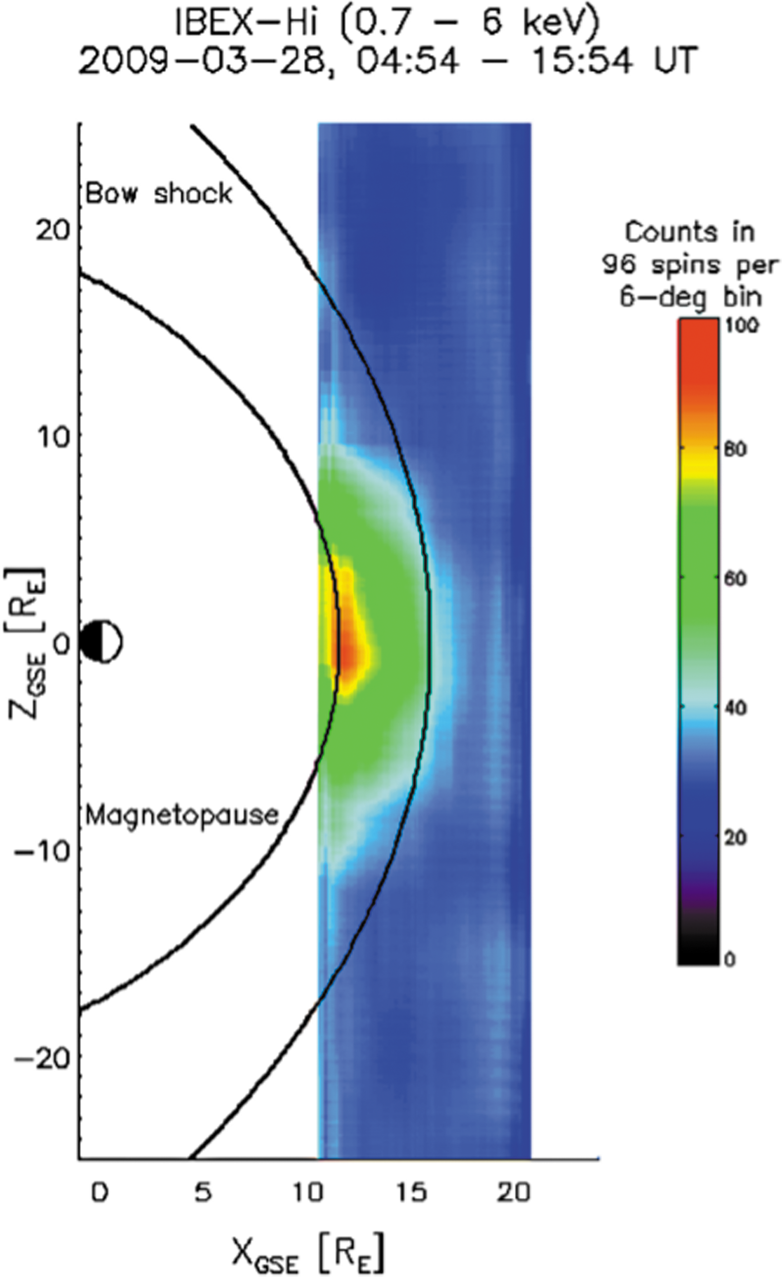
Observed hydrogen ENAs by the IBEX spacecraft around Earth. The H ENA count rate was integrated from 0.7 to 6 keV on March 28, 2009, from 04:54–15:54 UT. The peak is centered on the subsolar magnetopause, and a significant ENA flux extends to±10 R _Earth (Fuselier et al., 2010). Color images available online at www.liebertonline.com/ast

Before applying our model to hydrogen-rich exoplanets, we validated it by reproducing the geocorona and recent ENA observations (Fuselier et al., 2010) around Earth's magnetopause by NASA's IBEX satellite. Figure 2 shows our modeling results for Earth's geocorona interacting with the present-day solar wind by taking all parameters of Earth's exosphere as given in Table 1 as an input.

FIG. 2.

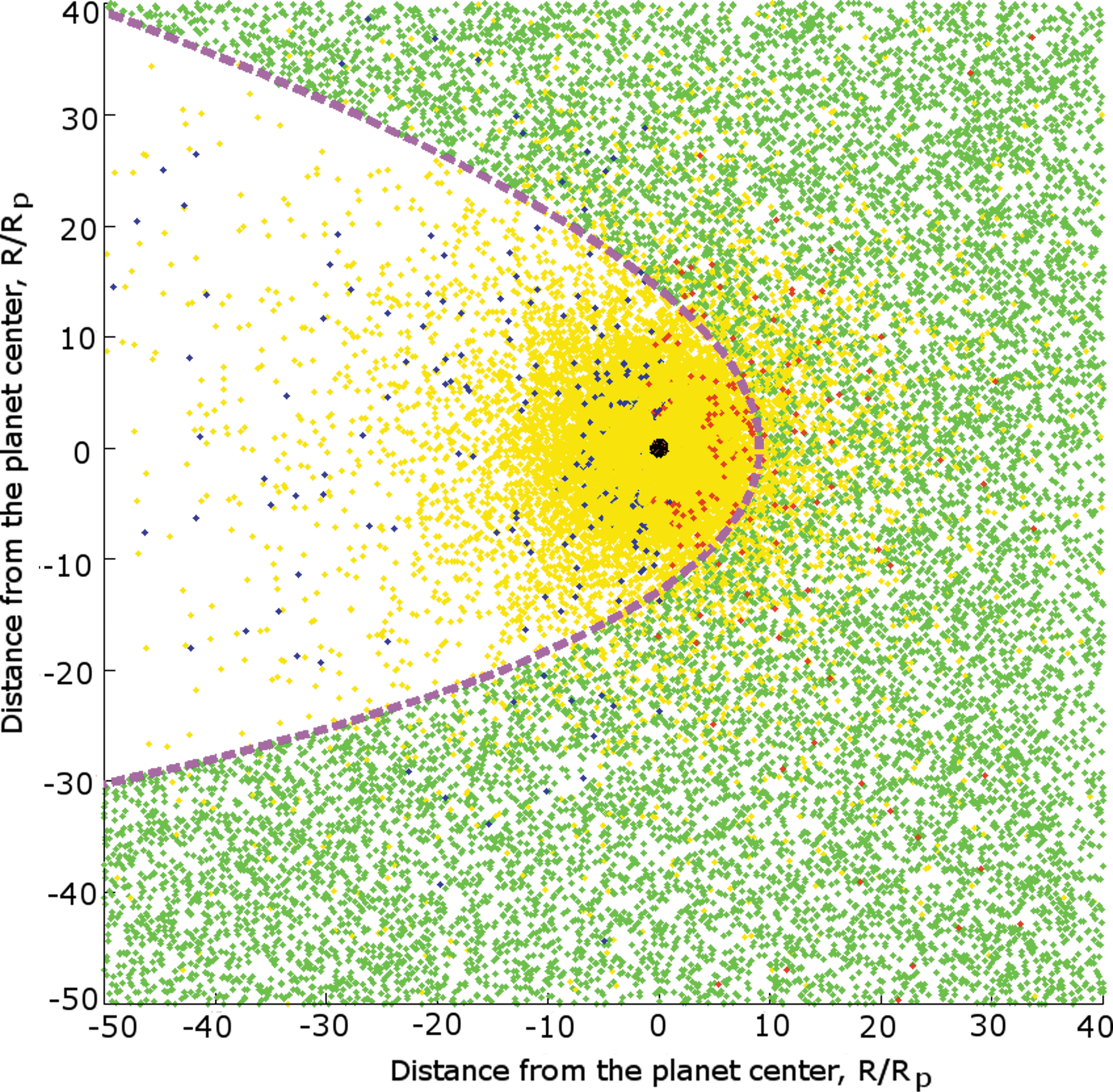
Modeling results of Earth's solar wind plasma interaction with the present-day geocorona. Green dots correspond to the solar wind protons, yellow dots represent the neutral hydrogen atoms moving with velocities below 10 km s⁻¹ (particles that belong to the atmosphere), while the red and the blue dots represent ENAs with velocities above 10 km s⁻¹, moving toward and away from the Sun, respectively. The dashed line denotes the magnetospheric obstacle. Color images available online at www.liebertonline.com/ast

Table 1.

Model Inner Boundary “ib” Atmospheric and Solar Wind Input Parameters for Present-Day Earth's Geocorona (Prölss, 2004)

R_ib [R_Earth ]	n_Hib [cm⁻³]	T_ib [K]	XUV_Sun	n_sw [cm⁻³]	v_sw [km s⁻¹]	T_sw [K]
1.078	7×10⁴	900	1	8	400	1×10⁶

The average neutral hydrogen atom density at the magnetopause level obtained from our model is estimated to be ∼8 cm⁻³ at the distance of ∼10 R _Earth. This density value coincides very well with the exospheric number densities inferred from the IBEX observations of ENAs near the magnetopause. In the case of the IBEX observation of March 28, 2009, the computed and observed proton fluxes show an exospheric hydrogen density at a geocentric distance of ∼10 R _Earth of ∼ 4–11 cm⁻³ (Fuselier et al., 2010). The estimates of the modeled ENA flux are in good agreement with the observed flux as well, predicting the flux of approximately 600 (cm² s sr keV)⁻¹. This value falls inside the observed ENA interval of ∼530–2300 (cm² s sr keV)⁻¹ (Fuselier et al., 2010).

The IBEX observation and our model validation can also be seen as a confirmation that, under the extreme radiation and plasma environments of the young Sun or of more active stars, a huge ENA formation zone, as suggested by Chassefière (1996) and Lammer et al. (2011b, 2013), should be produced in the stellar wind interaction region of a hydrogen-rich extended upper atmosphere of an Earth-sized planet when the exospheric density near the magnetopause is more than 10⁶ times larger than that observed at present-day Earth. In the following sections, we describe the input parameters and our applied exosphere and ENA models to the XUV-exposed hydrogen-rich Earth-sized test planets.

3. Gliese 436: A Host Star Proxy for Hydrogen-Rich Terrestrial Test Planets

3.1. The radiation environment of Gliese 436

Ehrenreich et al. (2011) observed with the Hubble Space Telescope Imaging Spectrograph (HST/STIS) the Lyman-α emission (1215.67 Å) of neutral hydrogen atoms from the low-mass M star GJ 436. Because this emission is a main contributor to the UV flux, it can also be used as a main tracer in studies of thermospheric heating, thermal escape, and possible absorption by extended hydrogen coronae and/or ENAs (e.g., Vidal-Madjar et al., 2003; Holmström et al., 2008; Ben-Jaffel and Sona Hosseini, 2010; Ekenbäck et al., 2010; Lecavelier des Etangs et al., 2010; Lammer et al., 2011b; Ehrenreich et al., 2012, Lammer, 2013) during transit observations with UV transmission spectroscopy. We used GJ 436 as a typical M type host star for our test-planet parameter studies. GJ 436 is an M2.5 dwarf star that is 10.2 pc away from the Sun. The dwarf star hosts a transiting “hot Neptune” at an orbital distance of about 0.03 AU (Butler et al., 2004; Gillon et al., 2007). We adopt values for stellar mass and radius of 0.45 M _Sun and 0.45 R _Sun, respectively, which are consistent with several independent parameter determinations of GJ 436 (Maness et al., 2007; Torres, 2007; von Braun et al., 2012). The location of the HZ is calculated following Selsis et al. (2007). As their relations are only valid for effective temperatures down to 3700 K, this value is used instead of the true temperature of GJ 436, which is slightly lower (3400–3600 K; Torres, 2007; von Braun et al., 2012). Further, we adopt a bolometric luminosity of 0.026 L _Sun (Torres, 2007). This leads to a HZ extent of 0.12–0.36 AU, assuming the limit of 50% clouds, as is typical for Earth. Hence, the center of the HZ is located at 0.24 AU, which we adopt as the orbit of our hypothetical exo-Earth. The orbital period of an Earth analog planet within the HZ of GJ 436 corresponds to approximately 63.7 days, the orbital velocity to about 41 km s⁻¹, and the angular velocity to 1.14×10⁻⁶ rad s⁻¹. The age of GJ 436 is about 6±5 Gyr and is not well constrained (Torres, 2007). However, the rotation period of 48 days (Demory et al., 2007) yields an estimated age of 2.5–3 Gyr (Barnes, 2007; Engle and Guinan, 2011). This estimation is in agreement with the lack of chromospheric activity indicated by the presence of Hα in absorption spectra.

Gliese 436 has been detected by the ROSAT All-Sky Survey, which revealed an X-ray luminosity of log L _X=27.13 erg s⁻¹. Recent observations by the XMM-Newton spacecraft yielded a smaller value of only ∼25.96 erg s⁻¹ (Sanz-Forcada et al., 2011). We adopt the latter result because of the longer exposure time and better S/N of the XMM-Newton observations compared to ROSAT data. Using coronal models, Sanz-Forcada et al. (2011) extrapolated the stellar emission in the total XUV range (5–920 Å) and found log L _XUV=26.92 erg s⁻¹. Adopting this value and scaling it to the HZ center at 0.24 AU, we estimate an XUV flux of about 5.14 erg cm⁻² s⁻¹, comparable to the present solar XUV flux at 1 AU of 4.64 erg cm⁻² s⁻¹ (Ribas et al., 2005).

In the past, the stellar XUV flux, which was emitted from GJ 436, was certainly higher. The high-energy emission of young M dwarfs is saturated at log(L _X/L _bol) ∼−3 (e.g., Scalo et al., 2007); hence the maximum possible log(L _X) for GJ 436 is ∼29 erg s⁻¹. Assuming that the XUV emission of young stars occurs predominantly in X-rays because of their hotter coronae, the maximum XUV flux at the Earth-equivalent orbit around GJ 436 was roughly 700 erg cm⁻² s⁻¹, or ∼150 F _XUV,now.

Lyman-α emission of GJ 436 was detected by Ehrenreich et al. (2011), who used HST/STIS observations. They reconstructed the intrinsic stellar emission by correcting for interstellar medium absorption, leading to an apparent flux observed at Earth of ∼2.7±0.7×10⁻¹³ erg cm⁻² s⁻¹. Scaled to the HZ center, this yields ∼20.51 erg cm⁻² s⁻¹, a factor of ∼3.3 larger than the present solar value at 1 AU of 6.19 erg cm⁻² s⁻¹ (Ribas et al., 2005). France et al. (2013) reconstructed the intrinsic Lyman-α flux of GJ 436 by using a different approach. They obtained a value of 3.5×10⁻¹³ erg cm⁻² s⁻¹ with an uncertainty of about 15–30%, which is slightly higher than the value given by Ehrenreich et al. (2011) but is consistent with the errors. The relevant stellar parameters and the measured radiation properties used in the model simulations for various assumed XUV flux values of a GJ 436–type M dwarf are shown in Table 2.

Table 2.

Default Stellar Parameters as Well as Values of Constants Used in the Simulations

Stellar radius [R _Sun]	0.45
Stellar mass [M _Sun]	0.45
Habitable zone [AU]	0.12–0.36
Orbital distance [AU]	0.24
Angular velocity [rad s⁻¹]	1.14×10⁻⁶
Orbital period [days]	64
XUV flux exposure [XUV_Sun]	1 \| 10 \| 50 \| 100
UV absorption rate [s⁻¹]	3.9×10⁻³ \| 1.2×10⁻² \| 2.7×10⁻² \| 3.9×10⁻²
Photoionization rate [s⁻¹]	1.1×10⁻⁷ \| 1.1×10⁻⁶ \| 5.5×10⁻⁶ \| 1.1×10⁻⁵

The photoionization rates corresponding to the four XUV flux enhancement factors were scaled from the average present solar value at Earth (1.1×10⁻⁷ s⁻¹; Hodges, 1994; Bzowski, 2008) to the corresponding enhancement factors. The photoionization rate is usually calculated as the product of ionization cross section and spectral flux integrated over all wavelengths below the ionization threshold. Since full M star XUV spectra for different activity levels are currently not available, we assume that the present spectral energy distribution is equal to the solar one and scale it up by the constant factors given in Table 2.

The UV absorption rates correspond to the product of the photon flux at the center of the Lyman-α line and the total absorption cross-section (5.47×10⁻¹⁵ cm² Å; e.g., Quémerais, 2006). Adopting the reconstructed intrinsic line profile of Ehrenreich et al. (2011), the present value of the photon flux at the HZ center of GJ 436 is estimated to be ∼6.9×10⁻³ s⁻¹. To scale the Lyman-α flux and, hence, the absorption rate to higher XUV flux emission levels, we use the scaling between X-rays and Lyman-α from Ehrenreich et al. (2011). This assumes that L _X/L _bol≈L _XUV/L _bol and that the central Lyman-α flux scales approximately as the integrated line emission. The resulting absorption rates are also shown in Table 2.

3.2. Expected stellar wind plasma properties

Depending on the mass, size, and resulting luminosity of the host star, the corresponding scaled HZ location in the case of GJ 436 is at 0.24 AU. This is a much closer orbital distance compared to that of Earth (1 AU). As pointed out by Khodachenko et al. (2007), at orbital locations <0.5 AU, the flow of dense plasma related to stellar winds and coronal mass ejections (CMEs), energetic particle fluxes, and XUV radiation cannot be neglected. Depending on the stand-off distance of the planetary obstacle that forms when the stellar plasma flow is deflected around the planet, previous test particle model results of Lammer et al. (2007) indicate that CO₂-rich Earth-like exoplanets that have no or only weak magnetic moments may lose from tens to hundreds of bar of atmospheric pressure, or even their whole atmospheres, due to the CME-induced O⁺ ion pickup at orbital distances ≤0.2 AU.

Due to the uncertainties on the mass loss and related plasma outflow from M dwarfs, we assume in our study, as in Khodachenko et al. (2007) and Lammer et al. (2007), the plasma environment close to the stars obtained from solar observations. There exist a limited number of measurements of the mass loss rates for M stars (Wood et al., 2005; Ehrenreich et al., 2011), which in principle may be used for estimation of specific stellar wind density and velocity. For these stars, the mass loss rates are comparable or less than the mass loss rate of the Sun. At the same time, for the Sun we have a much better knowledge of the distribution and evolution of active solar regions and of the mass outflow in the form of solar wind and CMEs, which we use in the present study. Note that stellar wind density and/or velocity lower than the solar (assumed) values would reduce the portion of the produced and picked-up ions. Such a reduction would not change our main conclusion that the ion pickup loss makes up only several percent of the thermal loss, and the further results can be considered as an upper limit for ion pickup near an M dwarf like GJ 436.

For the accurate study of stellar-planetary interactions, a reliable model is needed that can simulate the propagation and evolution of the stellar wind plasma. For modeling the propagation and evolution of the stellar wind, we use the Versatile Advection Code (Toth, 1996). This model is able to simulate spatial and temporal evolution of the solar/stellar wind, as well as CMEs, from orbital distances ≥0.14 AU. The model includes a self-consistent Parker-type corotating magnetic field and is based on the solution of the set of the ideal (nonresistive) nonrelativistic magnetohydrodynamic equations (Toth, 1996). We use a spherical uniform computation domain, which occupies a radial distance region between 0.14<R<1 AU. The stellar wind in the model flows through the inner boundary of the computation domain at a semimajor axis location d=0.14 AU and propagates out through the outer radial boundary at d=1 AU. A self-consistent expanding stellar wind plasma flow under the conditions of a frozen-in, corotating, Parker-type, spiral magnetic field is numerically simulated (Odstrčil and Pizzo, 1999; Rucker et al., 2008).

The typical parameters of the expected flow of the stellar wind plasma at d=0.14 AU are imposed along the inner radial boundary (Odstrčil and Pizzo, 1999) with an initial proton concentration n ₀=500 cm⁻³, stellar wind proton temperature T ₀=500 kK, and a radial stellar wind velocity v _r0=300 km s⁻¹. For investigating the propagation of CMEs, in a second step the simulation of a CME cloud with an initial proton density n ₀=1000 cm⁻³, proton temperature T ₀=1700 kK, and a radial stellar wind velocity v _r0=600 km s⁻¹ is imposed at the inner boundary of the computation domain as a time-dependent injection of hot and dense plasma into the ambient stellar wind (Odstrčil and Pizzo, 1999; Odstrčil et al., 2004).

Figure 3 shows radial profiles of the maximum values of plasma parameters (n, v _r, T) during a solar analog CME event (dashed lines, Case II) for a typical M star with mass m _s ∼ 0.45 M _Sun and a rotation period 2.5 days, and those for the stellar wind itself (solid lines, Case I). Therefore, in the stellar wind plasma interaction modeling with the upper atmosphere, described below, two types of stellar plasma parameters that represent the lower limit (Case I) and upper limit (Case II) conditions at the HZ location of our test planets at 0.24 AU were used as inputs:

• Case I: n _sw=250 cm⁻³, v _sw=330 km/s, T _sw=10⁶ K,

• Case II: n _sw=700 cm⁻³, v _sw=550 km/s, T _sw=2×10⁶ K.

FIG. 3.

Radial profiles for density, velocity, and temperature as a function of orbital location in AU and of expected plasma properties of an ordinary stellar wind (solid lines) and during a CME event (dashed lines) on an M type star with a mass M _s ∼0.45 M _Sun and a rotation period of 2.5 days. For the simulation of stellar wind, the initial proton density at 0.1 AU n ₀=400 cm⁻³, temperature T ₀=500 kK, and radial stellar wind velocity v _r0=300 km s⁻¹ were taken. Simulation of a solar analog CME event uses the initial proton density n ₀=800 cm⁻³, proton temperature T ₀=1500 kK, and radial stellar wind velocity v _r0=600 km s⁻¹.

Here, n _sw corresponds to stellar wind concentration, v _sw denotes its bulk velocity, and T _sw stands for the stellar wind temperature. These values cover the predicted range for the expected stellar wind plasma parameters of GJ 436 at the HZ of the system. The upper limit (Case II) can also be considered as a proxy for modeling of frequent CME events in the system when the next CME plasma cloud hits the planet immediately after the previous one. We can estimate the recovery time of the planetary atmosphere after the CME event in a very simple way. Since the test planets considered in the article are not magnetized, we assume that the recovery speed coincides with the sound speed (or the speed of slow magnetoacoustic wave), so that \documentclass{aastex}\usepackage{amsbsy}\usepackage{amsfonts}\usepackage{amssymb}\usepackage{bm}\usepackage{mathrsfs}\usepackage{pifont}\usepackage{stmaryrd}\usepackage{textcomp}\usepackage{portland, xspace}\usepackage{amsmath, amsxtra}\pagestyle{empty}\DeclareMathSizes{10}{9}{7}{6}\begin{document}$$\tau_ { \rm CME } = R_t / c_s = R_t \left( \frac { \gamma k_ { \rm B } T_ { \rm exo } } { m_ { \rm H } } \right) ^ { - 1 / 2}$$\end{document} where R_t is the obstacle width, γ=5/3 is the ratio of the specific heats, k _B is the Boltzmann constant, m _H is the mass of a hydrogen atom, and T _exo is the exobase temperature. Taking the parameters from Tables 3 and 4 and depending on the characteristic size of the obstacle and the temperature, this time varies between approximately 7 and 14 hours for the Earth-type planet and 64 and 80 hours for the super-Earth.

Table 3.

Planetary Input Parameters Taken from Erkaev et al. (2013) for Different Stellar Wind Properties and XUV Fluxes That Correspond to That of the Present Sun and an XUV Enhancement Factor of about 100 Times for a Low Heating Efficiency η=15%

Parameter/Case	Earth-type planet, 1 XUV, Case I	Earth-type planet, 100 XUV, Case II	super-Earth, 1 XUV, Case I	super-Earth, 100 XUV, Case II
Inner boundary [R _pl]	7.4	18.8	3.5	13.0
Inner boundary T [K]	240	2310	100	2075
Obstacle stand-off distance [R _pl]	7.5	19	3.6	13.1
Obstacle width [R _pl]	15	28.5	5.3	19.6
Inner boundary density [cm⁻³]	7.75×10⁴	2.77×10⁴	7.25×10⁴	2.0×10⁴

Table 4.

Parameter/Case	Earth-type planet, 1 XUV, Case I	Earth-type planet, 100 XUV, Case II	super-Earth, 1 XUV, Case I	super-Earth, 100 XUV, Case II
Inner boundary [R _pl]	7.84	22.94	6.98	18.44
Inner boundary T [K]	260	4875	500	4050
Obstacle stand-off distance [R _pl]	8	23	7.0	18.5
Obstacle width [R _pl]	12	34.5	10.5	27.0
Inner boundary density [cm⁻³]	7.25×10⁴	2.5×10⁴	4.0×10⁴	1.5×10⁴

The next section is dedicated to the discussion of the obtained results and presents also the ion production rates for the hydrogen-rich Earth-like planet and the super-Earth.

4. Hydrogen Exospheres, ENA Production, and Ion Escape

In the following section, we consider the modification of the extended hydrogen exosphere due to the interaction of it with the stellar XUV and plasma flux. Because our hydrogen-rich test planets orbit within a typical M star HZ at ∼0.24 AU, they will be affected by tides. As was discussed by Khodachenko et al. (2007), tides arise because of the finite extension of the planetary body in the inhomogeneous gravitational field of its host star such that the continuous action of the tides will reduce the planetary rotation rate or may result in a synchronous rotation (Grießmeier et al., 2005).

The intrinsic magnetic field of a terrestrial planet is an essential factor for planetary protection from the ion pickup atmospheric loss process. As shown by Khodachenko et al. (2007) and Lammer et al. (2007), because of the close orbital location within M star HZs, the magnetospheric field of a terrestrial planet is more compressed due to the denser stellar wind impact compared with that of the solar wind at present-day Earth at 1 AU. In view of this fact, the radial distance of the extended exobase of an XUV-heated hydrogen-rich upper atmosphere will most likely coincide with the planetary magnetopause or ionopause distance (e.g., Lammer et al., 2009a, 2012; Lammer, 2013).

4.1. Input parameters and modeling results

As was briefly discussed in Section 3.2, the magnetic moments of terrestrial planets, and especially that of super-Earths within close orbital distances, are expected to be weak (e.g., Gaidos et al., 2010; Tachinami et al., 2011; Morard et al., 2011; Stamenković et al., 2011, 2012). This would lead to magnetospheres or ionospheres that are compressed toward the planet's expanded non-hydrostatic upper atmosphere by the strong dynamic ram pressure of the dense stellar wind plasma. On the other hand, if the exobase level expands beyond several planetary radii, it can also be expected that an Earth-type magnetosphere will not protect the exosphere (Fig. 5: Lammer et al., 2007; Fig. 6 right panel: Lammer et al., 2011a). Taking these considerations into account, the planetary obstacle most likely is located very close above the exobase level (Lammer et al., 2009b). Because the shape of the planetary obstacle affects the ENA production and resulting loss of planetary hydrogen ions, we also consider the influence of the obstacle width on the ion production rate and the upper atmospheric erosion.

In the first case, the magnetic obstacle width R_t in Eq. 5 was assumed to be 1.5 times greater than the magnetopause distance at substellar point. This relation and its resulting obstacle shape is close to the observed magnetosphere of present-day Earth and may occur if the planet has an intrinsic magnetic dynamo. In the second case, we choose R_s =R_t so that it resembles more closely a venusian-type planetary obstacle that may correspond to a planet with no magnetic field or only a very weak dynamo. By decreasing the planetary obstacle width, the ion production will significantly increase, such that a terrestrial planet with a venusian-type obstacle, where R_s ≈R_t , may lose larger amounts of atmospheric gas in ionized form (see Section 4.2). In the present study, we do not specify the magnetic moment of a planet but only choose a magnetospheric obstacle.

For illustrating the differences between the stellar wind plasma interaction with a hydrogen-rich terrestrial planet exposed to both a weak XUV flux and an extremely strong one, we irradiated the two test planets with the XUV flux of the present Sun (1 XUV) and with a 100 times higher XUV flux (100 XUV). Moreover, we investigated for these two XUV flux cases several stellar wind and obstacle scenarios. The main input parameters at the inner boundary of our simulation domain are shown for four selected cases in Tables 3 and 4. As was mentioned earlier, we applied the results obtained by Erkaev et al. (2013) to the upper atmosphere input parameters of our model. Erkaev et al. (2013) studied the thermosphere structure of a hydrogen-dominated Earth and a super-Earth (R _pl=2 R _Earth; M _pl=10 M _Earth) with a hydrodynamic upper atmosphere model, which solves the equations of mass, momentum, and energy conservation for low and high heating efficiencies, η of 15% and 40%, respectively. η defines the percentage of the incoming XUV energy that is transferred into heating of the neutral gas. Table 4 shows the same input parameters for our model for a hotter atmosphere corresponding to the upper atmosphere values of Erkaev et al. (2013) with η=40%.

As can be seen in Tables 3 and 4, the exobase distance that is chosen as our inner model boundary and the temperature increase with higher XUV fluxes. This behavior can be expected when taking into account a more intensive radiation flux from the parent star. Enhanced heating flux makes the scale height of the atmosphere increase, which in turn moves the exobase to a higher location. It can also be seen that an increase of the heating efficiency leads to an increase of the planet's obstacle standoff distances (which for the studied nonmagnetized planets practically coincides with the exobase) as well. Because of the expansion of the upper atmosphere under more extreme heating conditions (40%), the exobase densities are smaller in comparison to the 15% cases.

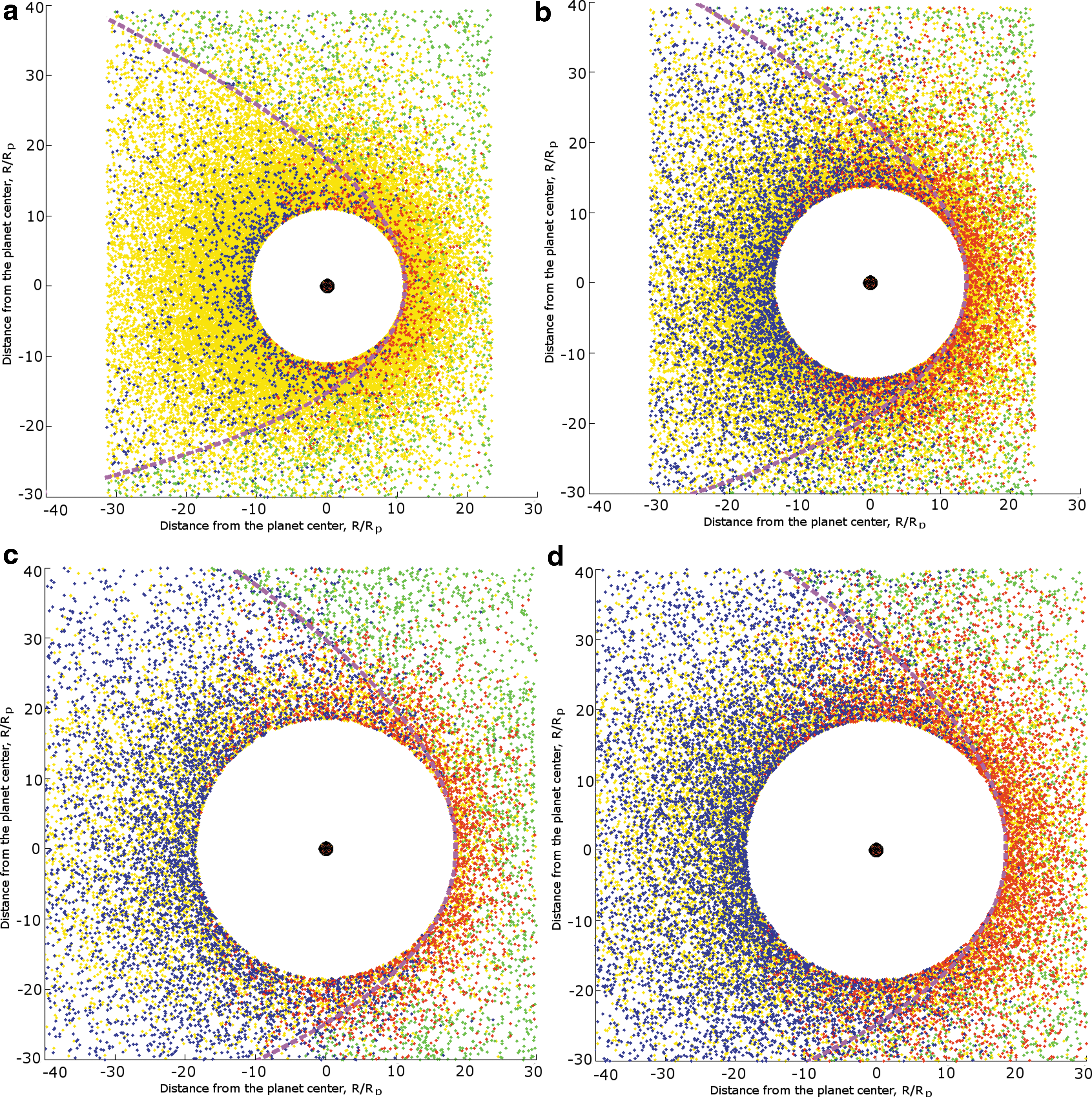
Figures 4 and 5 show the modeled hydrogen exospheres and the related stellar plasma interaction under various conditions around the test planets. All the figures show cross sections of a 3-D cloud in the x ₁, x ₂ plane similar to those in Fig. 2. Figure 4 illustrates the appearance of the extended hydrogen coronae around the Earth-type planet, while Fig. 5 corresponds to the super-Earth. In all cases, the wider Earth-type planetary obstacle is assumed, except for Fig. 4d where a smaller Venus-like obstacle is adopted.

FIG. 4.

Modeled atomic hydrogen coronae and stellar wind plasma interaction around an Earth-like hydrogen-rich planet inside an M star HZ at 0.24 AU (green, protons; yellow, H atoms; blue, ENAs flying away from the star; red, ENAs flying toward the star; dotted line, magnetopause/planetary obstacle). Figure (a) corresponds to the XUV flux, which is equal to that of the present Sun, the moderate stellar wind (Case I), and a lower heating efficiency of 15%. Figure (b) corresponds to the similar input parameters as in (a), but the XUV flux is 50 times higher. Figure (c) corresponds to the 10 times higher XUV flux than the present one and a heating efficiency of 15%, as well as the moderate stellar wind (Case I). Figure (d) corresponds to the similar input parameters as in (c) but for the venusian-type narrower planetary obstacle. Color images available online at www.liebertonline.com/ast

FIG. 5.

Modeled atomic hydrogen coronae and stellar wind plasma interaction around a super-Earth hydrogen-rich planet inside an M star HZ at 0.24 AU (green, protons; yellow, H atoms; blue, ENAs flying away from the star; red, ENAs flying toward the star; dotted line, magnetopause/planetary obstacle). (a) The XUV flux is 50 times higher than that of the present Sun, heating efficiency of 15%; the planet is exposed to a moderate stellar wind (Case I). (b) Similar conditions except for heating efficiency of 40%. (c) The XUV flux is 100 times higher compared to that of the present Sun, 40% heating efficiency, moderate stellar wind (Case I). (d) Similar input parameters as in (c) but exposed to a faster and denser stellar plasma flow (Case II). Color images available online at www.liebertonline.com/ast

The white area around the planets (which are shown as black dots) represents the inner atmosphere (non-hydrostatic thermosphere), which is not considered in the present study. Figures 4a and 4b illustrate the influence of the XUV flux on the cloud formation. All simulation parameters for these two pictures are the same except for the XUV flux, which is chosen to be equal to and 50 times higher than the XUV flux of the present Sun. As can be seen, the higher XUV flux leads to a more efficient expansion of the upper atmosphere so that charge exchange can be more intensive in the surrounding hydrogen corona. The effect of the planetary obstacle can be seen in a comparison of Fig. 4c, which shows an Earth-type planetary obstacle shape, with Fig. 4d, which shows a venusian-type obstacle. In these two cases, the upper atmosphere is exposed to an XUV flux that is 50 times higher compared to that of today's Sun.

Figures 5a and 5b illustrate the importance of the heating efficiency. We show two model runs for the super-Earth for a comparison. Only the upper-atmosphere parameters that correspond to the heating efficiencies were changed. A higher heating efficiency results in additional expansion of the upper atmosphere and in increasing production of ENAs in the vicinity of the planet (blue and red dots).

Figures 5c and 5d show the effect of the stellar wind velocity and density on the hydrogen coronae formation. Both figures, 5c and 5d, correspond to the most extreme XUV case, which is 100 times higher than that of today's Sun.

As expected, the extreme stellar conditions result in a denser and faster stellar plasma flow, higher XUV fluxes, and more intense heating of the upper atmosphere, as well as a decrease of the planetary obstacle width, all of which lead to more intensive interaction processes. The ENA part of the hydrogen corona (blue and red dots) becomes more visible, meaning an increase of the atmospheric erosion processes. It can be seen that a huge amount of exospheric hydrogen atoms is ionized or undergoes charge exchange reactions in both cases, but stronger stellar wind significantly increases the number of ENAs in the vicinity of the planet as suggested by Chassefière, (1996).

Chassefière (1996) studied the hydrodynamic outflow and escape of hydrogen atoms from a hydrogen-dominated expanded thermosphere from early Venus. From this study, it was estimated that the huge ENA cloud, which is generated via charge exchange due to the interaction between an extended exosphere and the surrounding solar wind plasma of the young Sun, may contribute to about 75% of the energy inside the thermosphere that is used for escape of the outward-flowing H atoms (see Fig. 3 in Chassefière, 1996). The stellar XUV flux is deposited mainly in the lower thermosphere (Erkaev et al., 2013), while the ENA flux directed toward the planet should be deposited at an atmospheric layer below the exobase. It can contribute to thermospheric heating and may as a consequence modify the upper atmosphere's structure, which could result in an enhancement of the thermal escape rate.

Our results related to the efficient production of ENAs around the planetary obstacle support the hypothesis of Chassefière (1996) that ENAs may contribute to upper atmospheric heating. Study of the possible additional heating contribution of ENAs to the stellar XUV flux is beyond the scope of this particular work but is in progress for a follow-up study in the near future. We note also that ENA clouds near the terrestrial exoplanets within orbits around M dwarfs might be observable in the stellar Lyman-α line by the Hubble Space Telescope and in higher resolution beyond the geocorona in the near future by the World Space Observatory-UV (Shustov et al., 2009; Lammer et al., 2011b).

In the next section, we estimate how many of the produced planetary ions in the hydrogen coronae are picked up by the stellar wind plasma and, hence, are lost from the planet.

4.2. Stellar wind–induced atmospheric erosion of planetary hydrogen ions

As discussed above, interaction processes between the stellar wind and the upper atmosphere together with the photoionization by stellar photons lead, in the case of hydrogen-rich atmospheres, to the production of atmospheric H⁺ ions; see Eq. 1. After ionization, the ions can be picked up by the stellar wind plasma and swept away from the planet. Because we are interested in the efficiency of the atmospheric ion escape, we estimate the average ion production rates under various conditions. We assume as discussed below that in the considered cases the production of planetary ions and the escape rate are most likely of the same order.

Ions produced near and above the planet's obstacle can be lost because of the ion pickup process. Since these particles are not neutral anymore, they can follow the magnetic field lines in the stellar wind plasma and can be swept away from the planet's gravity field. We consider the H⁺ ions produced above the planetary obstacle, where the collisions between atmospheric particles can be neglected. It is assumed that the ions may be lost if the gyro radius \documentclass{aastex}\usepackage{amsbsy}\usepackage{amsfonts}\usepackage{amssymb}\usepackage{bm}\usepackage{mathrsfs}\usepackage{pifont}\usepackage{stmaryrd}\usepackage{textcomp}\usepackage{portland, xspace}\usepackage{amsmath, amsxtra}\pagestyle{empty}\DeclareMathSizes{10}{9}{7}{6}\begin{document}\begin{align*}r_ { \rm g } = \frac { m_ { \rm i } v_ { \rm i } } { qB } , \tag { 6 } \end{align*}\end{document}

is small enough in comparison to the planetary radius (e.g., if the magnetic field in the vicinity of a planet is strong enough to change the trajectory of the ions significantly). Here, m _i is the mass of the ion, v _i is the velocity of the “cold” planetary ion assumed to be ∼7 km s⁻¹, q is the ion charge, and B is the magnetic field near the planetary obstacle. In the case of a pure hydrogen upper atmosphere, the ion mass and charge coincide with the mass and charge of a proton. The velocity of ∼7 km s⁻¹ is chosen as being slightly faster than the mean thermal velocity of a hydrogen atom for a temperature of about 2000 K. The magnetic field at the distance ∼0.24 AU from an M dwarf can be roughly estimated if a dipole character of the stellar field with the initial global value is assumed in the range of ∼2–3 kG or ∼0.2–0.3 T (Phan-Bao et al., 2009; Reiners, 2012). By assuming an average magnetic field on the star of 2 kG, the magnetic field at 0.24 AU is ≈1.4×10⁻³ G, which yields for an ion velocity of 7 km s⁻¹ an ion gyro radius of ∼525 m, which is several orders of magnitude smaller compared to the radii of the studied planets and especially to the radii of the exospheres. In such a case, it is justified to assume that most of the produced H⁺ ions will be swept away from the planets by the stellar wind. If we assume that the ions are accelerated by the stellar wind electric field to the velocity of the stellar wind (Case I: 330 km s⁻¹, Case II: 550 km s⁻¹), the ion gyro radius increases proportionally to ∼25–40 km in two extreme cases. Here, we assume the filling factor f=1 (see Phan-Bao et al., 2009), that is, the maximal possible field strength.

Since the magnetic field of ∼2–3 kG is typical for young and active M dwarfs, it would be convenient to determine the gyro radii for a weaker field of ∼50 G for an older star with the age of several billion years (Phan-Bao et al., 2009). The magnetic field at 0.24 AU is approximately 3.57×10⁻⁵ G. A decrease of the magnetic field causes a proportional increase of the gyro radius (21 km for an ion velocity of 7 km s⁻¹, 10³ and 1.6×10³ km for 330 and 550 km s⁻¹, respectively). But even the highest value of ∼1600 km is several times less if compared to the planetary radius and more than an order of magnitude lower compared to the exobase radius, which is where most ENAs are produced. These estimates support our assumption that the majority of the exospheric ions are lost from the planet and that the ion production rate is balanced by the escape rate at least during a significant part of the stellar lifetime.

Estimates of the ion production rates and corresponding escape rates described in the previous sections are summarized in Tables 5 and 6 for planetary obstacles that have an Earth-like magnetosphere shape. Table 5 presents the results obtained for a hydrogen-rich Earth-like planet for two stellar wind conditions and a heating efficiency η=15% and a higher heating efficiency η=40%, while Table 6 summarizes the similar scenarios for the super-Earth. Atmospheric loss rates L _ion are given in units of particles per second. As can be seen in Tables 5 and 6, the ion production and loss rate, in most cases, increase with the increasing XUV flux. Loss rates for faster stellar wind also exceed the corresponding values for the wind with lower velocity, which is not surprising. Since the ion production rates depend not only on the assumed heating efficiency and the XUV flux but also on the exobase density, the values for the lower-density case corresponding to a heating efficiency of 40% (Erkaev et al., 2013) are slightly lower in comparison to the 15% case shown in Table 6.

Table 5.

Ion Escape Rates L _ion in s ⁻¹ for a Hydrogen-Rich Earth-like Planet and for a Heating Efficiency of 15%, Exposed to the XUV Flux Values, Which Are 1, 10, 50, and 100 Times Higher Than That of the Present Sun

H-rich Earth	1 XUV	10 XUV	50 XUV	100 XUV
Case I, η=15%	1.35×10²⁹	6.32×10²⁹	1.03×10³⁰	1.59×10³⁰
Case I, η=40%	2.60×10²⁹	1.58×10³⁰	1.40×10³⁰	1.57×10³⁰
Case II, η=15%	2.15×10²⁹	9.50×10²⁹	1.54×10³⁰	2.55×10³⁰
Case II, η=40%	4.11×10²⁹	2.17×10³⁰	2.04×10³⁰	2.40×10³⁰

The shape of the planetary obstacle is assumed to be similar to an Earth-type magnetosphere.

Table 6.

Ion Escape Rates L _ion in s ⁻¹ for a Hydrogen-Rich Super-Earth for a Heating Efficiency of 15% and 40%, Exposed to the XUV Flux Values, Which Are 1, 10, 50, and 100 Times Higher Than That of the Present Sun

H-rich super-Earth	1 XUV	10 XUV	50 XUV	100 XUV
Case I, η=15%	1.03×10²⁵	4.64×10²⁹	9.86×10²⁹	1.66×10³⁰
Case I, η=40%	8.62×10²⁸	9.50×10²⁹	9.71×10²⁹	1.22×10³⁰
Case II, η=15%	2.60×10²⁵	8.18×10²⁹	1.57×10³⁰	2.79×10³⁰
Case II, η=40%	1.62×10²⁹	1.55×10³⁰	1.59×10³⁰	2.80×10³⁰

The shape of the planetary obstacle is assumed to be similar to an Earth-type magnetosphere.

This is also the reason why the values for the cases where the stellar XUV flux is about 100 times higher than that of the present Sun are not dramatically higher (or even slightly smaller) than the ion production rates for the lower XUV fluxes, although the intensity of the interaction increases. Under the intensity of the interaction in this case, we mean the ratio of produced ions to the mean exospheric density. This value increases monotonically for higher XUV fluxes in all cases considered in the present study. The reason for this is related to the corresponding exobase density that is lower because of expansion in the case of a hydrogen-rich upper atmosphere that is exposed to high XUV fluxes such as in the 100 XUV case (Erkaev et al., 2013).

To investigate the influence of the planetary obstacle shape on the H⁺ escape rate L _ion, we performed an analogous set of simulations by assuming a venusian-type planetary obstacle (R_s ≈R_t ). Tables 7 and 8 present the calculated ion production rates and estimated ion escape rates for the two test planets under the same conditions as described in Tables 5 and 6 except for the shape of the planetary obstacle. As can be seen from the comparison of Tables 5–6 and Tables 7–8, reducing the width of the obstacle by 1.5 times leads to an increase in the ion production rate (i.e., the escape in general) of ≈30%. Other factors that lead to an increase of the ion production rate are increase of the stellar wind density and velocity, heating efficiency η, and enhancement of the stellar XUV flux of the parent star. All these dependencies should be considered as expected.

Table 7.

Ion Escape Rates L _ion in s ⁻¹ for a Hydrogen-Rich Earth-like Planet for a Heating Efficiency of 15% and 40%, Exposed to the XUV Flux Values, Which Are 1, 10, 50, and 100 Times Higher Compared to That of the Present Sun

H-rich Earth	1 XUV	10 XUV	50 XUV	100 XUV
Case I, η=15%	2.75×10²⁹	9.02×10²⁹	1.33×10³⁰	2.14×10³⁰
Case I, η=40%	3.72×10²⁹	1.97×10³⁰	1.89×10³⁰	2.54×10³⁰
Case II, η=15%	5.05×10²⁹	1.0×10³⁰	2.23×10³⁰	2.97×10³⁰
Case II, η=40%	6.27×10²⁹	3.23×10³⁰	3.84×10³⁰	4.15×10³⁰

The shape of the planetary obstacle is assumed to be Venus-like.

Table 8.

Ion Escape Rates L _ion in s ⁻¹ for a Hydrogen-Rich Super-Earth for a Heating Efficiency of 15% and 40%, Exposed to the XUV Flux Values, Which Are 1, 10, 50, and 100 Times Higher Compared to That of the Present Sun

H-rich super-Earth	1 XUV	10 XUV	50 XUV	100 XUV
Case I, η=15%	4.81×10²⁷	8.47×10²⁹	1.59×10³⁰	2.74×10³⁰
Case I, η=40%	2.31×10²⁹	1.48×10³⁰	1.69×10³⁰	2.33×10³⁰
Case II, η=15%	1.23×10²⁸	1.38×10³⁰	2.62×10³⁰	4.10×10³⁰
Case II, η=40%	5.17×10²⁹	2.36×10³⁰	2.87×10³⁰	5.36×10³⁰

The shape of the planetary obstacle is assumed to be Venus-like.

For comparison, thermal loss rates change in the range from 4.0×10²⁹ (1 XUV, η=15%) to 4.3×10³¹ (100 XUV, η=40%) for a hydrogen-rich Earth-type planet and from 1.6×10²⁹ (1 XUV, η=15%) to 5.3×10³¹ (100 XUV, η=40%) for a hydrogen-rich super-Earth. In all cases, these rates exceed that presented in the current study. For more information, see Erkaev et al. (2013).

If we compare the modeled H⁺ ion pickup loss rates with that of Mars (e.g., Lammer et al., 2003) or Venus (Lammer et al., 2006), which are of the order of ∼10²⁵ s⁻¹, it can be seen that the pickup loss rates for the hydrogen-dominated Earth-like planet are comparable for the 1 XUV case with a heating efficiency of 15% and an Earth-like magnetopause shape but would be a factor of 10³ higher in the case of 40% heating efficiency and/or a narrower venusian-type planetary obstacle. For the larger super-Earth and XUV cases with higher values than that of the present-day Sun, the loss rates are up to 10⁴ to 10⁵ times higher.

4.3. Total ion escape

The loss rates shown in Tables 5 –8 can be used for rough estimation of the total ion loss from the hydrogen envelopes around the studied planets. This question is important because, as shown by Erkaev et al. (2013), volatile-rich super-Earths that contain IR-cooling molecules can result in lower heating efficiencies of about 15% so that for most of their lifetime they will not be in the hydrodynamic blow-off regime. In such cases, nonthermal atmospheric escape processes, like the studied H⁺ ion pickup process, will contribute to the loss of their hydrogen-rich protoatmospheres.

Before investigating this mass loss, we need to know how long a typical M dwarf like GJ 436 can keep a high level of the XUV and X-ray flux. According to Penz et al. (2008a), the temporal scaling law for the soft X-ray (0.6–12.4 nm or 0.1–2 keV) flux of a typical M dwarf with the mass of ≈0.4 M _Sun can be described by the following relation: \documentclass{aastex}\usepackage{amsbsy}\usepackage{amsfonts}\usepackage{amssymb}\usepackage{bm}\usepackage{mathrsfs}\usepackage{pifont}\usepackage{stmaryrd}\usepackage{textcomp}\usepackage{portland, xspace}\usepackage{amsmath, amsxtra}\pagestyle{empty}\DeclareMathSizes{10}{9}{7}{6}\begin{document}\begin{align*} \begin{split}L_{ \rm X} ( t \leq 0.6 \ { \rm Gyr} ) & \approx 0.17L_0 t^{ - 0.77} , \ L_{ \rm X} ( t > 0.6 \ { \rm Gyr} ) \\& \approx 0.13 L_0 t^{ - 1.34} ,\end{split} \tag{7}\end{align*}\end{document}

where L ₀=5.6×10²⁸ erg s⁻¹ and t is given in billions of years. The soft X-ray flux can then be scaled for the appropriate orbital distance by using the relation F _X=L _X/4πd ².

Figure 6 shows, approximately, the decrease of the soft X-ray flux of a GJ 436 analogous M dwarf during the first 1.3 Gyr of its lifetime. Since at present time the scaling law for the XUV radiation of M dwarfs is not yet well constrained, we use this soft X-ray scaling law instead of the XUV scaling law in our estimation for the total H⁺ escape. Assuming this temporal scaling law for the star and taking the ion production rates from Tables 5 –8, we can estimate the mass loss from the hydrogen-rich Earth-like planet and the super-Earth in the HZ of a GJ 436–type M star after 4.5 Gyr (see Tables 9 and 10). For comparison, the thermal escape rates are shown by using the values from Table 2 in Erkaev et al. (2013).

FIG. 6.

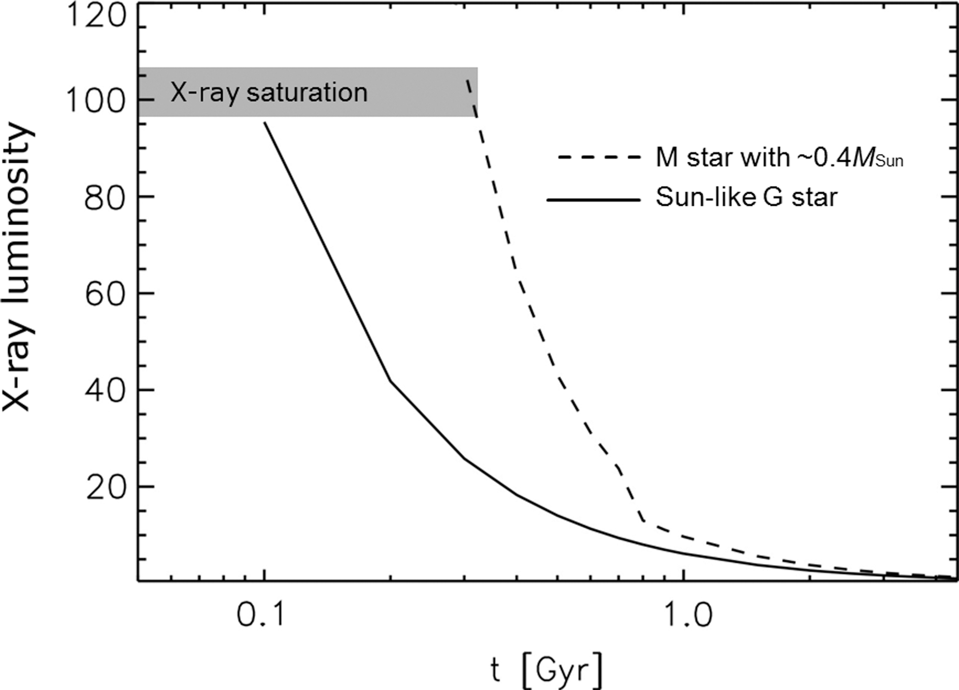
Illustration of the soft X-ray flux time dependence for an M dwarf star with 0.4 solar masses (dashed line) and the same curve for a Sun-like star (solid line) in the corresponding HZs normalized by the present solar flux. The M star within this mass range remains about 200 Myr longer in its activity saturation phase compared to a Sun-like G star.

Table 9.

Thermal (L _th) and Nonthermal (L _ion, H⁺ Ion Pickup) Loss Over the Time Span of 4.5 Gyr for a H-Rich Earth-like Planet and a H-Rich Super-Earth, Orbiting an M Dwarf in the Habitable Zone at 0.24 AU, by Considering an Earth-Type Magnetosphere Shape for the Planetary Obstacle Form and the Low and High Heating Efficiency of 15% and 40%

H loss: Δt=4.5 Gyr	H-rich Earth [EO_H]	H-rich super-Earth [EO_H]
L _th: η=15%	∼7.0	∼2.2
L _th: η=40%	∼16	∼8.0
L _ion: η=15%, Case I	∼0.6	∼0.41
L _ion: η=15%, Case II	∼0.93	∼0.7
L _ion: η=40%, Case I	∼1.13	∼0.64
L _ion: η=40%, Case II	∼1.63	∼1.44

Table 10.

Nonthermal (L _ion, H⁺ Ion Pickup) Loss Over the Time Span of 4.5 Gyr for a H-Rich Earth-like Planet and a H-Rich Super-Earth, Orbiting an M Dwarf in the Habitable Zone at 0.24 AU, by Considering a Venusian-Type Planetary Obstacle Shape and the Low and High Heating Efficiency of 15% and 40%

H loss: Δt=4.5 Gyr	H-rich Earth [EO_H]	H-rich super-Earth [EO_H]
L _ion: η=15%, Case I	∼0.92	∼0.71
L _ion: η=15%, Case II	∼1.24	∼1.13
L _ion: η=40%, Case I	∼1.51	∼1.15
L _ion: η=40%, Case II	∼2.56	∼2.14

The total ion loss is given in Earth ocean equivalent amounts of hydrogen (1 EO_H=1.5×10²³ g). It should also be mentioned that we do not consider escape during the first ∼100 Myr, the time of extreme stellar activity of an M dwarf, so that our estimates cover the time span ∼0.1–4.5 Gyr. As discussed by Erkaev et al. (2013), the temperature in the lower thermosphere during this early extreme period may be >>250 K due to magma oceans and frequent impacts. A hot lower atmosphere will enhance the atmospheric thermal escape during this early period. A follow-up study that will investigate the earliest extreme evolutionary periods is in progress.

In the present work, we do not take into account the gradual decrease of the amount of gas in the planetary atmosphere due to escape processes, as we assume that the hydrogen reservoir contains much more gas in comparison to the amount lost. As discussed in Section 1, such scenarios can be considered as real because most of the recently discovered super-Earths may have huge hydrogen envelopes that contain a few percent of their whole mass (e.g., Lammer, 2013).

If we compare the estimated atmospheric escape rates obtained for the thermal and ion pickup processes for both test planets in the HZ, it is clear that the thermal escape rate substantially exceeds the pickup rate under the studied conditions. This is also the case when we consider the most extreme XUV and stellar plasma conditions, including a narrow planetary obstacle. A fraction of the evaporating neutral exosphere will be ionized, so ion pickup will contribute to the total atmospheric escape rate. However, as long as the upper atmosphere is in blow-off, thermal escape will be most important.

In our study, the escape rate of ionized hydrogen atoms can vary for an Earth-type planet from ∼0.6 EO_H under moderate conditions (15% heating efficiency, moderate stellar wind, Earth-type planetary obstacle) up to ∼2.5 EO_H for extreme environments (40% heating efficiency, denser and faster wind, and a narrow venusian obstacle type).

The stronger gravity of the more massive super-Earth keeps the atmosphere closer to the planet's surface, which slows down the charge exchange and photoionization processes. In this case, the escape changes from ∼0.4 EO_H to ∼2.14 EO_H, depending on the environment, but remains smaller compared to escape from an Earth-type planet (ranging from ∼0.6 EO_H to 2.5 EO_H, see above). In all studied cases, the nonthermal H⁺ pickup rate is several times smaller in comparison with the thermal one but makes up a significant fraction of the whole loss processes.

The results of our study, together with those of Erkaev et al. (2013), indicate that terrestrial exoplanets that range in mass and size from Earth to super-Earths may not lose dense hydrogen envelopes if they have H-dominated protoatmospheric remnants with >9 EO_H (Earth: η=15%) and >19 EO_H (Earth: η=40%). For a super-Earth, these amounts are >3.5 EO_H (η=15%) and >10 EO_H (η=40%). Dense hydrogen envelopes may be removed more easily if a particular exoplanet is located closer to its parent star such as Corot-7b or Kepler-10b (e.g., Leitzinger et al., 2011), which orbit their parent stars at ∼0.017 AU but not inside the HZ. We note also that, due to the HZ location at greater distances from the parent stars, the stellar wind erosion of hydrogen envelopes will be less efficient for planets inside the HZs of K, G, and F type stars.

5. Conclusions

In this study, we investigated the nonthermal ion pickup escape process from hydrogen-rich, non-hydrostatic upper atmospheres of an Earth-like planet and a hydrogen-rich super-Earth that is twice as large as Earth and 10 times more massive. Both planets are supposed to be located inside the HZ of a typical M dwarf star with stellar properties similar to those of GJ 436. We showed that in the case of an M dwarf the produced planetary H⁺ ions have a high probability to be picked up from the extended hydrogen coronae by the stellar wind plasma flow such that the ion production rate and the ion escape rate are perhaps of the same order. We exposed the two test planets to various XUV fluxes from 1 to 100 times that of the present Sun and found that in all studied cases the ionization of exospheric neutral hydrogen atoms by charge exchange and photoionization contributes to the total atmospheric escape of the upper atmosphere but does not prevail over the thermal escape. The total nonthermal atmospheric escape by ion pickup from possible dense hydrogen envelopes during the lifetime of the studied planets is <3 EO_H. Our results indicate that if a rocky exoplanet does not lose the majority of its nebula-captured hydrogen gas envelope or degassed a huge amount of hydrogen-rich volatiles by thermal blow-off during the first hundred million years after the planet's origin, it is questionable as to whether the stellar wind can erode a remaining dense hydrogen envelope nonthermally. The thermal escape is higher during the planet's history but is probably unable to remove such dense hydrogen envelopes as well. The situation may change dramatically for exoplanets that are located closer to their parent stars. Depending on the nebula lifetime, the formation process, planetary mass, stellar activity, and plasma properties in the vicinity of the planet, the initial amount of hydrogen, thermal and nonthermal atmospheric escape processes will determine whether a planet becomes a world with an Earth-type atmosphere (and no hydrogen envelope) or remains a sub-Neptune–type body.

Footnotes

Acknowledgments

M. Güdel, K.G. Kislyakova, M.L. Khodachenko, and H. Lammer acknowledge support by the FWF NFN project S116 “Pathways to Habitability: From Disks to Active Stars, Planets and Life,” and the related FWF NFN subprojects, S116 604-N16 “Radiation & Wind Evolution from T Tauri Phase to ZAMS and Beyond,” S116 606-N16 “Magnetospheric Electrodynamics of Exoplanets,” S11 6607-N16 “Particle/Radiative Interactions with Upper Atmospheres of Planetary Bodies Under Extreme Stellar Conditions.” K.G. Kislyakova, Yu.N. Kulikov, H. Lammer, and P. Odert thank also the Helmholtz Alliance project “Planetary Evolution and Life.” P. Odert and M. Leitzinger acknowledge support from the FWF project P22950-N16. The authors also acknowledge support from the EU FP7 project IMPEx (No. 262863) and the EUROPLANET-RI projects, JRA3/EMDAF and the Na2 science WG5. The authors thank the International Space Science Institute (ISSI) in Bern and the ISSI team “Characterizing stellar- and exoplanetary environments.” Finally, N.V. Erkaev acknowledges support by the RFBR grant No. 12-05-00152-a. This research was conducted using resources provided by the Swedish National Infrastructure for Computing (SNIC) at the High Performance Computing Center North (HPC2N), Umeå University, Sweden. The software used in this work was in part developed by the DOE-supported ASC/Alliance Center for Astrophysical Thermonuclear Flashes at the University of Chicago. Finally, the authors thank the referees for very useful suggestions and recommendations which helped to improve the work.

Abbreviations

CMEs, coronal mass ejections; DSMC, Direct Simulation Monte Carlo; ENA, energetic neutral atom; HST/STIS, Hubble Space Telescope Imaging Spectrograph; HZ, habitable zone; IBEX, Interstellar Boundary Explorer.

References

Barnes

S.A.

2007. Ages for illustrative field stars using gyrochronology: viability, limitations, and errors. Astrophys J, 669:1167–1189.

Ben-Jaffel

, Sona Hosseini

2010. On the existence of energetic atoms in the upper atmosphere of exoplanet HD 209458b. Astrophys J, 709:1284–1296.

Bonfils

, Delfosse

, Udry

, Forveille

, Mayor

, Perrier

, Bouchy

, Gillon

, Lovis

, Pepe

, Queloz

, Santos

N.C.

, Ségransan

, Bertaux

J.-L.

2013. The HARPS search for southern extra-solar planets XXXI. The M dwarf sample. Astron Astrophys 10.1051/0004-6361/201014704.

Butler

R.P.

, Vogt

S.S.

, Marcy

G.W.

, Fischer

D.A.

, Wright

J.T.

, Henry

G.W.

, Laughlin

, Lissauer

J.J.

2004. A Neptune-mass planet orbiting the nearby M dwarf GJ 436. Astrophys J, 617:580–588.

Bzowski

2008. Survival probability and energy modification of hydrogen energetic neutral atoms on their way from the termination shock to Earth orbit. Astron Astrophys, 488:1057–1068.

Chandrasekhar

1963. The equilibrium and the stability of the Roche ellipsoids. Astrophys J, 138:1182–1213.

Charbonneau

, Berta

Z.K.

, Irwin

, Burke

C.J.

, Nutzman

, Buchhave

L.A.

, Lovis

, Bonfils

, Latham

D.W.

, Udry

, Murray-Clay

R.A.

, Holman

M.J.

, Falco

E.E.

, Winn

J.N.

, Queloz

, Pepe

, Mayor

, Delfose

, Forveille

2009. A super-Earth transiting a nearby low-mass star. Nature, 462:891–894.

Chassefière

1996. Hydrodynamic escape of hydrogen from a hot water-rich atmosphere: the case of Venus. J Geophys Res, 101:26039–26056.

Chassefière

, Leblanc

2004. Mars atmospheric escape and evolution; interaction with the solar wind. Planet Space Sci, 52:1039–1058.

10.

Chaufray

J.Y.

, Modolo

, Leblanc

, Chanteur

, Johnson

R.E.

, Luhmann

J.G.

2007. Mars solar wind interaction: formation of the martian corona and atmospheric loss to space. J Geophys Res, 112. 10.1029/2007JE002915.

11.

Demory

B.-O.

, Gillon

, Barman

, Bonfils

, Mayor

, Mazeh

, Queloz

, Udry

, Bouchy

, Delfosse

, Forveille

, Mallmann

, Pepe

, Perrier

2007. Characterization of the hot Neptune GJ 436 b with Spitzer and ground-based observations. Astron Astrophys, 475:1125–1129.

12.

Dressing

C.D.

, Charbonneau

2013. The occurrence rate of small planets around small stars. Astrophys J, 767. 10.1088/0004-637X/767/1/95.

13.

Ehrenreich

, Lecavelier des Etangs

, Delfosse

2011. HST/STIS Lyman-α observations of the quiet M dwarf GJ 436. Predictions for the exospheric transit signature of the hot Neptune GJ 436b. Astron Astrophys, 529:A80.

14.

Ehrenreich

, Bourrier

, Bonfils

, Lecavelier des Etangs

, Hébrard

, Sing

D.K.

, Wheatley

P.J.

, Vidal-Madjar

, Delfosse

, Udry

, Forveille

, Moutou

2012. Hint of a transiting extended atmosphere on 55 Cancri b. Astron Astrophys, 547:A18.

15.

Ekenbäck

, Holmström

, Wurz

, Grießmeier

J.-M.

, Lammer

, Selsis

, Penz

2010. Energetic neutral atoms around HD 209458b: estimations of magnetospheric properties. Astrophys J, 709:670–679.

16.

Elkins-Tanton

L.T.

2011. Formation of water ocean on rocky planets. Astrophys Space Sci, 332:359–364.

17.

Endl

, Robertson

, Cochran

W.D.

, MacQueen

P.J.

, Brugamyer

E.J.

, Caldwell

, Wittenmyer

R.A.

, Barnes

S.I.

, Gullikson

2012. Revisiting ρ¹ Cancri e: a new mass determination of the transiting super-Earth. Astrophys J, 759. 10.1088/0004-637X/759/1/19.

18.

Engle

S.G.

, Guinan

E.F.

2011. Red dwarf stars: ages, rotation, magnetic dynamo activity and the habitability of hosted planets. Astronomical Society of the Pacific Conference Series, 451:285–296.

19.

Erkaev

N.V.

, Penz

, Lammer

, Lichtenegger

H.I.M.

, Wurz

, Biernat

H.K.

, Griessmeier

J.-M.

, Weiss

W.W.

2005. Plasma and magnetic field parameters in the vicinity of short periodic giant exoplanets. Astrophys J, 157:396–401.

20.

Erkaev

N.V.

, Lammer

, Odert

, Kulikov

Yu.N.

, Kislyakova

K.G.

, Khodachenko

M.L.

, Güdel

, Hanslmeier

, Biernat

H.K.

2013. XUV-exposed, non-hydrostatic hydrogen-rich upper atmospheres of terrestrial planets. Part I: atmospheric expansion and thermal escape. Astrobiology, 13. 10.1089/ast.2012.0957.

21.

Fox

J.L.

, Hać

A.B.

2009. Photochemical escape of oxygen from Mars: a comparison of the exobase approximation to a Monte Carlo method. Icarus, 204:527–544.

22.

France

, Froning

C.S.

, Linsky

J.L.

, Roberge

, Stocke

J.T.

, Tian

, Bushinsky

, Desert

J.-M.

, Mauas

, Vieytes

, Walcowicz

L.M.

2013. The ultraviolet radiation environment around M dwarf exoplanet host stars. Astrophys J, 763. 10.1088/0004-637X/763/2/149.

23.

Fryxell

, Olson

, Picker

, Timmes

F.X.

, Zingale

, Lamb

D.Q.

, MacNeice

, Rosner

, Truran

J.W.

, Tufo

2000. FLASH: an adaptive MESH hydrodynamic code for modeling astrophysical thermonuclear flashes. Astrophys J Supplement Series, 131:273–334.

24.

Fuselier

S.A.

, Funsten

H.O.

, Heirtzler

, Janzen

, Kucharek

, McComas

D.J.

, Möbius

, Moore

T.E.

, Petrinec

S.M.

, Reisenfeld

D.B.

, Schwadron

N.A.

, Trattner

K.J.

, Wurz

2010. Energetic neutral atoms from the Earth's subsolar magnetopause. Geophys Res Lett, 77:L13101.

25.

Futaana

, Barabash

, Grigoriev

, Holmström

, Kallio

, son Brandt

P.C.

, Gunell

, Brinkfeldt

, Lundin

, Andersson

, Yamauchi

, McKenna-Lawler

, Winningham

J.D.

, Frahm

R.A.

, Sharber

J.R.

, Scherrer

J.R.

, Coates

A.J.

, Linder

D.R.

, Kataria

D.O.

, Säles

, Riihelä

, Schmidt

, Koskinen

, Kozyra

, Luhmann

, Roelof

, Williams

, Livi

, Curtis

C.C.

, Hsieh

K.C.

, Sandel

B.R.

, Grande

, Carter

, Sauvaud

J.-A.

, Fedorov

, Thocaven

J.-J.

, Orsini

, Cerulli-Irelli

, Maggi

, Wurz

, Bochsler

, Galli

, Krupp

, Woch

, Fränz

, Asamura

, Dierker

2006. First ENA observations at Mars: subsolar ENA jet. Icarus, 182:413–423.

26.

Gaidos

, Condrad

C.P.

, Manga

, Hernlund

2010. Thermodynamic limits on magnetodynamos in rocky exoplanets. Astrophys J, 718:598–609.

27.

Galli

, Wurz

, Bochsler

, Barabash

, Grigoriev

, Futaana

, Holmström

, Gunell

, Andersson

, Lundin

, Yamauchi

, Brinkfeldt

, Fränz

, Krupp

, Woch

, Baumjohann

, Lammer

, Zhang

T.L.

, Asamura

, Coates

A.J.

, Linder

D.R.

, Kataria

D.O.

, Curtis

C.C.

, Hsien

K.C.

, Sandel

B.R.

, Sauvaud

J.A.

, Fedorov

, Mazelle

, Thocaven

J.J.

, Grande

, Kallio

, Sales

, Schmidt

, Riihela

, Koshkinen

, Kozyra

, Luhmann

, McKenna-Lawlor

, Orsini

, Cerulli-Irelli

, Mura

, Milillo

, Maggi

, Roelof

, Brandt

, Russel

C.T.

, Szego

, Winningham

, Frahm

, Scherrer

, Sharber

J.R.

2008. First observation of energetic neutral atoms in the Venus environment. Planet Space Sci, 56:807–811.

28.

García Muñoz

2007. Physical and chemical aeronomy of HD 209458b. Planet Space Sci, 55:1426–1455.

29.

Gillon

, Pont

, Demory

B.-O.

, Mallmann

, Mayor

, Mazeh

, Queloz

, Shporer

, Udry

, Vuissoz

2007. Detection of transits of the nearby hot Neptune GJ 436 b. Astron Astrophys, 472:L13–L16.

30.

Grießmeier

J.-M.

, Stadelmann

, Motschmann

, Belisheva

N.K.

, Lammer

, Biernat

H.K.

2005. Cosmic ray impact on extrasolar Earth-like planets in close-in habitable zones. Astrobiology, 5:587–603.

31.

Gröller

, Shematovich

V.I.

, Lichtenegger

H.I.M.

, Lammer

, Pfleger

, Kulikov

Yu.N.

, Macher

, Amerstorfer

U.V.

, Biernat

H.K.

2010. Venus' atomic hot oxygen environment. J Geophys Res, 115. 10.1029/2010JE003697.

32.

Gröller

, Lammer

, Lichtenegger

H.I.M.

, Pfleger

, Dutuit

, Shematovich

V.I.

, Kulikov

Yu.N.

, Biernat

H.K.

2012. Hot oxygen atoms in the Venus nightside exosphere. Geophys Res Lett, 39:L03202.

33.

Hayashi

, Nakazawa

, Mizuno

1979. Earth's melting due to the blanketing effect of the primordial dense atmosphere. Earth Planet Sci Lett, 43:22–28.

34.

Hodges

R.R.

Jr.

1994. Monte Carlo simulation of the terrestrial hydrogen exosphere. J Geophys Res, 99:23229–23247.

35.

Holmström

, Ekenbäck

, Selsis

, Penz

, Lammer

, Wurz

2008. Energetic neutral atoms as the explanation for the high-velocity hydrogen around HD 209458b. Nature, 451:970–972.

36.

Ikoma

, Genda

2006. Constraints on the mass of a habitable planet with water of nebular origin. Astrophys J, 648:696–706.

37.

Ikoma

, Hory

2012. In situ accretion of hydrogen-rich atmospheres on short-period super-Earths: implications for the Kepler-11 planets. Astrophys J, 753. 10.1088/0004-637X/753/1/66.

38.

Johnson

R.E.

1990. Energetic Charged Particle Interactions with Atmospheres and Surfaces. Springer: Berlin.

39.

Kasting

J.F.

, Pollack

J.B.

1983. Loss of water from Venus. I. Hydrodynamicc escape of hydrogen. Icarus, 53:479–509.

40.

Khodachenko

M.L.

, Ribas

, Lammer

, Grießmeier

J.-M.

, Leitner

, Selsis

, Eiroa

, Hanslmeier

, Biernat

, Farrugia

C.J.

, Rucker

2007. Coronal mass ejection (CME) activity of low mass M stars as an important factor for the habitability of terrestrial exoplanets. I. CME impact on expected magnetospheres of Earth-like exoplanets in close-in habitable zones. Astrobiology, 7:167–184.

41.

Korenaga

2010. On the likelihood of plate tectonics on super-Earths: does size matter? Astrophys J, 725:L43–L46.

42.

Koskinen

T.T.

, Harris

M.J.

, Yelle

R.V.

, Lavvas

2013. The escape of heavy atoms from the ionosphere of HD209458b. I. A photochemical-dynamical model of the thermosphere. Icarus, 226:1678–1694.

43.

Krestyanikova

M.A.

, Shematovich

V.I.

2005. Stochastic models of hot planetary and satellite coronas: a photochemical source of hot oxygen in the upper atmosphere of Mars. Solar System Research, 39:22–32.

44.

Krestyanikova

M.A.

, Shematovich

V.I.

2006. Stochastic models of hot planetary and satellite coronas: a hot oxygen corona of Mars. Solar System Research, 40:384–392.

45.

Kuchner

M.J.

2003. Volatile-rich Earth-mass planets in the habitable zone. Astrophys J, 596:L105–L108.

46.

Lammer

2013. Origin and Evolution of Planetary Atmospheres: Implications for Habitability, Springer Briefs in Astronomy. Springer: Berlin.

47.

Lammer

, Lichtenegger

H.I.M.

, Kolb

, Ribas

, Guinan

E.F.

, Bauer

S.J.

2003. Loss of water from Mars: implications for the oxidation of the soil. Icarus, 165:9–25.

48.

Lammer

, Lichtenegger

H.I.M.

, Biernat

H.K.

, Erkaev

N.V.

, Arshukova

I.L.

, Kolb

, Gunell

, Lukyanov

, Holmstrom

, Barabash

, Zhang

T.L.

, Baumjohann

2006. Loss of hydrogen and oxygen from the upper atmosphere of Venus. Planet Space Sci, 54:1445–1456.

49.

Lammer

, Lichtenegger

H.I.M.

, Kulikov

Yu.N.

, Grießmeier

J.-M.

, Terada

, Erkaev

N.V.

, Biernat

H.K.

, Khodachenko

M.L.

, Ribas

, Penz

, Selsis

2007. Coronal mass ejection (CME) activity of low mass M stars as an important factor for the habitability of terrestrial exoplanets. II. CME-induced ion pick-up of Earth-like exoplanets in close-in habitable zones. Astrobiology, 7:185–207.

50.

Lammer

, Bredehöft

J.H.

, Coustenis

, Khodachenko

M.L.

, Kaltenegger

, Grasset

, Prieur

, Raulin

, Ehrenfreund

, Yamauchi

, Wahlund

J.-E.

, Grießmeier

J.-M.

, Stangl

, Cockell

C.S.

, Kulikov

Y.N.

, Grenfell

J.L.

, Rauer

. 2009a. What makes a planet habitable? Astron Astrophys, 17:181–249.

51.

Lammer

, Odert

, Leitzinger

, Khodachenko

M.L.

, Panchenko

, Kulikov

Yu.N.

, Zhang

T.L.

, Lichtenegger

H.I.M.

, Erkaev

N.V.

, Wuchterl

, Micela

, Penz

, Biernat

H.K.

, Weingrill

, Steller

, Ottacher

, Hasiba

, Hanslmeier

2009b. Determining the mass loss limit for close-in exoplanets: what can we learn from transit observations? Astron Astrophys, 506:399–410.

52.

Lammer

, Kislyakova

K.G.

, Odert

, Leitzinger

, Schwarz

, Pilat-Lohinger

, Kulikov

Yu.N.

, Khodachenko

M.L.

, Güdel

, Hanslmeier

2011a. Pathways to Earth-like atmospheres: extreme ultraviolet (EUV)-powered escape of hydrogen-rich protoatmospheres. Orig Life Evol Biosph, 41:503–522.

53.

Lammer

, Eybl

, Kislyakova

K.G.

, Weingrill

, Holmström

, Khodchenko

M.L.

, Kulikov

Yu.N.

, Reiners

, Leitzinger

, Odert

, Xian Grüß

, Dorner

, Güdel

, Hanslmeier

2011b. UV transit observations of EUV-heated expanded thermospheres of Earth-like exoplanets around M-stars: testing atmosphere evolution scenarios. Astrophys Space Sci, 335:39–50.

54.

Lammer

, Güdel

, Kulikov

Yu.N.

, Zaqarashvili

T.V.

, Khodachenko

M.L.

, Kislyakova

K.G.

, Gröller

, Odert

, Leitzinger

, Fichtinger

, Krauss

, Hausleitner

, Holmström

, Sanz-Forcada

, Lichtenegger

H.I.M.

, Hanslmeier

, Shematovich

V.I.

, Bisikalo

, Rauer

, Fridlund

2012. Variability of solar/stellar activity and magnetic field and its influence on planetary atmosphere evolution. Earth, Planets and Space, 64,2:179–199.

55.

Lammer

, Erkaev

N.V.

, Odert

, Kislyakova

K.G.

, Leitzinger

, Khodachenko

M.L.

2013. Probing the blow-off criteria of hydrogen-rich “super-Earths.” Mon Not R Astron Soc, 430:1247–1256.

56.

Leblanc

, Johnson

R.E.

2002. Role of molecular species in pick-up ion sputtering of the martian atmosphere. J Geophys Res, 107:1–6.

57.

Lecavelier des Etangs

, Ehrenreich

, Vidal-Madjar

, Ballester

G.E.

, Désert

J.-M.

, Ferlet

, Hébrard

, Sing

D.K.

, Tchakoumegni

K.-O.

, Udry

2010. Evaporation of the planet HD 189733b observed in H I Lyman-α Astron Astrophys, 514:A72.

58.

Léger

, Selsis

, Sotin

, Guillot

, Despois

, Mawet

, Ollivier

, Labèque

, Valette

, Brachet

, Chazelas

, Lammer

2004. A new family of planets? “Ocean-planets.” Icarus, 169:499–504.

59.

Leitzinger

, Odert

, Kulikov

Yu.N.

, Lammer

, Wuchterl

, Penz

, Guarcello

M.G.

, Micela

, Khodachenko

M.L.

, Weingrill

, Hanslmeier

, Biernat

H.K.

, Schneider

2011. Could CoRoT-7b and Kepler-10b be remnants of evaporated gas or ice giants? Planet Space Sci, 59:1472–1481.

60.

Lichtenegger

H.I.M.

, Lammer

, Grießmeier

J.-M.

, Kulikov

Yu.N.

, von Paris

, Hausleitner

, Krauss

, Rauer

2010. Aeronomical evidence for higher CO₂ levels during Earth's Hadean epoch. Icarus, 210:1–7.

61.

Linsky

J.L.

, Yang

, France

, Froning

C.S.

, Green

J.C.

, Stocke

J.T.

, Osterman

S.N.

2010. Observations of mass loss from the transiting exoplanet HD 209458b. Astrophys J, 717:1291–1299.

62.

Lissauer

J.J.

, Fabrycky

D.C.

, Ford

E.B.

, Borucki

W.J.

, Fressin

, Marcy

G.W.

, Orosz

J.A.

, Rowe

J.F.

, Torres

, Welsh

W.F.

, Batalha

N.M.

, Bryson

S.T.

, Buchhave

L.A.

, Caldwell

D.A.

, Carter

J.A.

, Charbonneau

, Christiansen

J.L.

, Cochran

W.D.

, Desert

J.-M.

, Dunham

E.W.

, Fanelli

M.N.

, Fortney

J.J.

, Gautier

T.N.

III , Geary

J.C.

, Gilliland

R.L.

, Haas

M.R.

, Hall

J.R.

, Holman

M.J.

, Koch

D.G.

, Latham

D.W.

, Lopez

, McCauliff

, Miller

, Morehead

R.C.

, Quintana

E.V.

, Ragozzine

, Sasselov

, Short

D.R.

, Steffen

J.H.

2011. A closely packed system of low-mass, low-density planets transiting Kepler-11. Nature, 470:53–58.

63.

Lundin

, Lammer

, Ribas

2007. Planetary magnetic fields and solar forcing: implications for atmospheric evolution. Space Sci Rev, 129:245–278.

64.

Y.-J.

, Nagy

A.F.

2007. Ion escape fluxes from Mars. Geophys Res Lett, 34:L08201.

65.

Maness

H.L.

, Marcy

G.W.

, Ford

E.B.

, Hauschildt

P.H.

, Shreve

A.T.

, Basri

G.B.

, Butler

R.P.

, Vogt

S.S.

2007. The M Dwarf GJ 436 and its Neptune-mass planet. Publ Astron Soc Pac, 119:90–101.

66.

Mizuno

, Nakazawa

, Hayashi

1978. Instability of a gaseous envelope surrounding a planetary core and formation of giant planets. Progress of Theoretical Physics, 60:699–710.

67.

Morard

, Bouchet

, Valencia

, Mazevet

, Guyot

2011. The melting curve of iron at extreme pressures: implications for planetary cores. High Energy Density Physics, 7:141–144.

68.

Möstl

U.V.

, Erkaev

N.V.

, Zellinger

, Lammer

, Gröller

, Biernat

H.K.

, Korovinskiy

2011. The Kelvin-Helmholtz instability at Venus: what is the unstable boundary? Icarus, 216:476–484.

69.

Murray-Clay

R.A.

, Chiang

E.I.

, Murray

2009. Atmospheric escape from hot Jupiters. Astrophys J, 693:23–42.

70.

Odstrčil

, Pizzo

V.J.

1999. Three-dimensional propagation of CMEs in a structured solar wind flow: 1. CME launched within the streamer belt. J Geophys Res, 104,A1:483–492.

71.

Odstrčil

, Riley

, Zhao

X.P.

2004. Numerical simulation of the 12 May 1997 interplanetary CME event. J Geophys Res, 109,A2:A0211.

72.

Penz

, Erkaev

N.V.

, Biernat

H.K.

, Lammer

, Amerstorfer

U.V.

, Gunell

, Kallio

, Barabash

, Orsini

, Milillo

, Baumjohann

2004. Ion loss on Mars caused by the Kelvin-Helmholtz instability. Planet Space Sci, 52:1157–1167.

73.

Penz

, Michela

, Lammer

2008a. Influence of the evolving stellar X-ray luminosity distribution on exoplanetary mass loss. Astron Astrophys, 477:309–314.

74.

Penz

, Erkaev

N.V.

, Kulikov

Y.N.

, Langmayr

, Lammer

, Micela

, Cecchi-Pestellini

, Biernat

H.K.

, Selsis

, Barge

, Deleuil

, Léger

2008b. Mass loss from “Hot Jupiters”—implications for CoRoT discoveries, part II: long time thermal atmospheric evaporation modeling. Planet Space Sci, 56:1260–1272.

75.

Phan-Bao

, Lim

, Donati

J.-F.

, Johns-Krull

C.M.

, Martin

E.L.

2009. Magnetic field topology in low-mass stars: spectropolametric observations of M dwarfs. Astrophys J, 704:1721–1729.

76.

Prölss

G.W.

2004. Physik des erdnahen Weltraums. Springer: Berlin.

77.

Quémerais

2006. The interplanetary Lyman α background. The Physics of the Heliospheric Boundaries, ISSI Scientific Report No. 5. Izmodenov

V.V.

, Kallenbach

International Space Science Institute: Bern, 283–310.

78.

Rafikov

R.R.

2006. Atmospheres of protoplanetary cores: critical mass for nucleated instability. Astrophys J, 648:666–682.

79.

Reiners

2012. Observations of cool-star magnetic fields. Living Reviews in Solar Physics, 9. 10.12942/lrsp-2012-1.

80.

Ribas

, Guinan

E.F.

, Güdel

, Audard

2005. Evolution of the solar activity over time and effects on planetary atmospheres. I. High-energy irradiances (1–1700 Å) Astrophys J, 622:680–694.

81.

Rucker

H.O.

, Panchenko

, Hansen

K.C.

, Taubenschluss

, Boudjada

M.Y.

, Kurth

W.S.

, Dougherty

M.K.

, Steinberg

J.T.

, Zarka

, Galopeau

P.H.M.

, McComas

D.J.

, Barrow

C.H.

2008. Saturn kilometric radiation as a monitor for the solar wind? Adv Space Res, 42:40–47.

82.

Sanz-Forcada

, Micela

, Ribas

, Pollock

A.M.T.

, Eiroa

, Velasco

, Solano

, García-Álvarez

2011. Estimation of the XUV radiation onto close planets and their evaporation. Astron Astrophys, 532:A6.

83.

Scalo

, Kaltenegger

, Segura

A.G.

, Fridlund

, Ribas

, Kulikov

Yu.N.

, Grenfell

J.L.

, Rauer

, Odert

, Leitzinger

, Selsis

, Khodachenko

M.L.

, Eiroa

, Kasting

, Lammer

2007. M stars as targets for terrestrial exoplanet searches and biosignature detection. Astrobiology, 7:85–166.

84.

Selsis

, Kasting

J.F.

, Levrard

, Paillet

, Ribas

, Delfosse

2007. Habitable planets around the star Gliese 581? Astron Astrophys, 476:1373–1387.

85.

Shematovich

V.I.

2010. Suprathermal hydrogen produced by the dissociation of molecular hydrogen in the extended atmosphere of exoplanet HD 209458b. Solar System Research, 44:96–103.

86.

Shustov

, Sachov

, Gomez de Castro

A.I.

, Ana

, Pagano

2009. WSO-UV ultraviolet mission for the next decade. Astrophys Space Sci, 320:187–190.

87.

Stamenković

, Breuer

, Spohn

2011. Thermal and transport properties of mantle rock at high pressure: applications to super-Earths. Icarus, 216:572–596.

88.

Stamenković

, Noack

, Breuer

, Spohn

2012. The influence of pressure-dependent viscosity on the thermal evolution of super-Earths. Astrophys J, 748. 10.1088/0004-637X/748/1/41.

89.

Tachinami

, Senshu

, Ida

2011. Thermal evolution and lifetime of intrinsic magnetic fields of super-Earths in habitable zones. Astrophys J, 726. 10.1088/0004-637X/726/2/70.

90.

Terada

, Machida

, Shinagawa

2002. Global hybrid simulation of the Kelvin-Helmholtz instability at the Venus ionopause. J Geophys Res, 107:1471–1490.

91.

Tian

, Toon

O.B.

, Pavlov

A.A.

, De Sterck

2005a. Transonic hydrodynamic escape of hydrogen from extrasolar planetary atmospheres. Astrophys J, 621:1049–1060.

92.

Tian

, Toon

O.B.

, Pavlov

A.A.

, De Sterck

2005b. A hydrogen-rich early Earth atmosphere. Science, 308:1014–1017.

93.

Tian

, Kasting

J.F

, Liu

, Roble

R.G.

2008a. Hydrodynamic planetary thermosphere model: 1. The response of the Earth's thermosphere to extreme solar EUV conditions and the significance of adiabatic cooling. J Geophys Res, 113:E05008.

94.

Tian

, Solomon

S.C.

, Qian

, Lei

, Roble

R.G.

2008b. Hydrodynamic planetary thermosphere model: 2. Coupling of an electron transport/energy deposition model. J Geophys Res, 113. 10.1029/2007JE003043.

95.

Torres

2007. The transiting exoplanet host star GJ 436: a test of stellar evolution models in the lower main sequence, and revised planetary parameters. Astrophys J, 671:L65–L68.

96.

Toth

1996. A general code for modeling MHD flows on parallel computers: versatile advection code. Astrophysical Letters and Communications, 34:245–250.

97.

Valencia

, O'Connell

R.J.

, Sasselov

D.D.

2007. Inevitability of plate tectonics on super-Earths. Astrophys J, 670:L45–L48.

98.

van Heck

H.J.

, Tackley

P.J.

2011. Plate tectonics on super-Earths: equally or more likely than on Earth. Earth Planet Sci Lett, 310:252–261.

99.

Vidal-Madjar

, Lecavelier des Etangs

, Désert

J.M.

, Ballester

G.E.

, Ferlet

, Hébrard

, Mayor

2003. An extended upper atmosphere around the extrasolar planet HD209458b. Nature, 422:143–146.

100.

Volkov

A.N.

, Johnson

R.E.

, Tucker

O.J.

, Erwin

J.T.

2011. Thermally driven atmospheric escape: transition from hydrodynamic to Jeans escape. Astrophys J, 729:L24.

101.

von Braun

, Boyajian

T.S.

, Kane

S.R.

, Hebb

, van Belle

G.T.

, Farrington

, Ciardi

D.R.

, Knutson

H.A.

, ten Brummelaar

T.A.

, López-Morales

, McAlister

H.A.

, Schaefer

, Ridgway

, Collier Cameron

, Goldfinger

P.J.

, Turner

N.H.

, Sturmann

2012. The GJ 436 system: directly determined astrophysical parameters of an M dwarf and implications for the transiting hot Neptune. Astrophys J, 753. 10.1088/0004-637X/753/2/171.

102.

Watson

A.J.

, Donahue

T.M.

, Walker

J.C.G.

1981. The dynamics of a rapidly escaping atmosphere—applications to the evolution of Earth and Venus. Icarus, 48:150–166.

103.

Wei

, Fraenz

, Dubinin

, Woch

, Lühr

, Wan

, Zong

Q.-G.

, Zhang

T.-L.

, Pu

Z.Y.

, Fu

S.Y.

, Barabash

, Lundin

, Dandouras

2012. Enhanced atmospheric oxygen outflow on Earth and Mars driven by a corotating interaction region. J Geophys Res, 117:A03208.

104.

Wood

B.E.

, Müller

H.-R.

, Zank

G.P.

, Linksky

J.L.

, Redfield

2005. New mass-loss measurements from atmospheric Lyα absorption. Astrophys J, 628:L143–L146.

105.

Wuchterl

1993. The critical mass for protoplanets revised—massive envelopes through convection. Icarus, 106:323–334.

106.

Yau

A.W.

, André

1997. Sources of ion outflow in the high latitude ionosphere. Space Sci Rev, 37:1–25.

107.

Yelle

R.V.

2004. Aeronomy of extra-solar giant planets at small orbital distances. Icarus, 170:167–179.

108.

Yelle

2006. Corrigendum to “Aeronomy of extra-solar giant planets at small orbital distances” [Icarus 170 (2004) 167–179] Icarus, 183:508.