Field Demonstration of an Instrument Performing Automatic Classification of Geologic Surfaces

Abstract

This work presents a method with which to automate simple aspects of geologic image analysis during space exploration. Automated image analysis on board the spacecraft can make operations more efficient by generating compressed maps of long traverses for summary downlink. It can also enable immediate automatic responses to science targets of opportunity, improving the quality of targeted measurements collected with each command cycle. In addition, automated analyses on Earth can process large image catalogs, such as the growing database of Mars surface images, permitting more timely and quantitative summaries that inform tactical mission operations. We present TextureCam, a new instrument that incorporates real-time image analysis to produce texture-sensitive classifications of geologic surfaces in mesoscale scenes. A series of tests at the Cima Volcanic Field in the Mojave Desert, California, demonstrated mesoscale surficial mapping at two distinct sites of geologic interest. Key Word: Interpretation of planetary mission data. Astrobiology 14, 486–501.

1. Introduction

To date, ongoing Mars rover missions have accumulated an archive of just under 380,000 microscopic and macroscopic images: 309,680 over 10 years for the Mars Exploration Rover mission and 68,131 for the Mars Science Laboratory in a year. This is the result of increased mission survivability, mobility, and autonomy. It can be assumed that archives will grow even larger in future missions due to continuing progress in technology and instrumentation (Furgale and Barfoot, 2010; Bakambu et al., 2012) as well as in science operation productivity (Deans et al., 2012). Standard now on Mars rovers (Squyres et al., 2003; Grotzinger et al., 2012) and planned for the Mars 2020 mission (Mustard et al., 2013), multiscale imaging allows a science team to generate powerful nested imagery to characterize morphological, mineralogical, and compositional domains to submeter resolution while simultaneously mapping them on a scale of tens of kilometers. However, analysis bottlenecks, such as limited downlink bandwidth and limited analyst time, can prevent missions from fully utilizing these data for tactical operations planning. The present work describes image analysis algorithms and instrument hardware that can automate rudimentary aspects of geologic analysis both on the ground and on board spacecraft. Simple automatic visual processing of these images can improve the efficiency of mission operations as well as the ultimate science yield.

A primary challenge for Mars surface mission operations is the limited time the science team can afford to spend daily on data analysis. The team must quickly analyze data downlinks while simultaneously deciding on the next science targets and designing traverse plans—all within the handful of hours before the next uplink window. Both targets and traverses are chosen based on the highest priorities of the science team. In most cases, a science team will preferentially collect and analyze the data that best support the primary mission science objectives (e.g., for high-impact publications and communications) and will only later have time for an in-depth review of the archived data. As a result, it often takes many years for data archives to be fully investigated. Some observations may never be fully analyzed, which can create a potential gap in mission productivity. The earlier and more rigorous the quantitative analysis, the better informed later exploration decisions can be. Timely analysis is especially critical for rover missions, since there is little chance of revisiting sites once the mission is over. Further, missions rarely return to previously investigated targets during mission operations, due to a general perception that a mission only makes progress if it goes forward—perhaps to explore as many diverse environments as possible in a limited, unknown mission life span. This is, so far, a clear distinction between robotic exploration and terrestrial fieldwork, where revisiting sites and resampling are not only common but often critical.

In such context, the use of efficient autonomous analytical image techniques can increase the scientific impact of large archives during operations. It could be particularly valuable for a mission such as the Mars 2020 mission, a central goal of which will be to seek signs of early life on Mars and identify a high-value subset of samples to prepare for a later sample return mission. More than for any previous mission, this objective requires (a) an especially careful contextual mapping of large traversed areas in order to understand the stratigraphic context of samples and discoveries; (b) the ability to investigate and interpret as critical or noncritical numerous sedimentary landforms and their remnants (from residual mesoscale features to rocks and particulates), whether layered or nonlayered, and in situ or not; (c) the capability to identify textural groups that may bear evidence of potential fossil biogenic constructs from others that may not; and (d) the analytical power to investigate the textural, morphological, and compositional elements of a scene that can provide information on the energy of transportation and on depositional environments in the explored region.

Automated image analysis can also improve exploration efficiency by performing simple data interpretation on board the spacecraft (Gulick et al., 2001; Woods et al., 2009, 2011). Missions such as the Mars 2020 mission may spend a considerable fraction of the mission performing long drives and reconnaissance, passing through terrain that has only been seen previously from orbit. It is important that missions retain the flexibility to respond to targets of opportunity and deploy targeted remote sensing or contact instruments as needed without stalling the mission or incurring the delay of an extra command cycle. Onboard image analysis allows the spacecraft to respond immediately to these unanticipated targets, for example, by directing high-resolution cameras or targeted spectroscopy at novel rocks or stratigraphic features (McGuire et al., 2010). This idea was the core of the AEGIS system, which provided computer vision for automatic science feature selection by the Mars Exploration Rover Opportunity (Estlin et al., 2012). A simple visual analysis can also allow more effective targeted measurements upon arrival at a destination outcrop. Specifically, automatic mesoscale maps can indicate the principal units of material for a representative remote measurement. The same analysis can also show good locations for contact sensing that are free of dust or fractures. These simple image analyses can save critical command cycles and latency required for Earth operators to micromanage each approach, surface evaluation, and placement maneuver. Finally, surface classification products can be downlinked to provide information about terrain the rover has passed when bandwidth constraints prevent downlinking complete images. In these ways, automated image analysis offers a path to address key operations bottlenecks and improve the science return of the mission over its finite operational lifetime.

The following sections present TextureCam, an instrument that incorporates built-in automatic image analysis. The techniques we describe can improve the analytical power and decision making of future missions by allowing (1) surficial mapping over a much larger area than is currently possible, including maps produced for tactical decisions during science operations, and (2) onboard automated mapping that will make autonomous planetary rovers more efficient. To address the second goal, we have built this capability into embedded sensor hardware. The result is a camera system that can classify surfaces in real time—a smart instrument that we demonstrated in field trials at relevant geologic sites in the Cima Volcanic Field of the Mojave Desert, California. These tests show the feasibility of real-time image analysis and provide a rough picture of expected system performance for some simple surface classification tasks. This work focuses on real-time image analysis in mesoscale scenes, which we define as containing features generally greater than 64 mm in size (anything smaller falls into “gravel” or “sediment” category). Automatic classification of rocks on the microscopic scale has also shown good results (Mlynarczuk et al., 2013).

2. Approach

This section describes our technical approach, beginning with a brief description of the image analysis algorithm and then explaining our instrument hardware implementation.

2.1. Algorithm

We formulate the problem of geologic image analysis as pixel classification in which the system categorizes image regions based on predefined labels. This does not capture all geologic image analysis tasks, but we find it to be a general and flexible formulation that can accommodate many or most of the stated objectives. The pixel categories may represent geologic content such as layering (Thompson et al., 2011; Wagstaff et al., 2013), rock surfaces (Wagstaff et al., 2013; Francis et al., 2014), and particle sizes. Alternatively, they could involve nongeologic attributes like illumination and shadow (Foil et al., 2013) or operations objectives such as identifying physical surfaces in good condition for contact sensing (Wagstaff et al., 2013). This formulation is therefore broad enough to encompass a wide range of autonomous activities and image analyses in support of long-range traverse science. For example, simple postprocessing applied to pixel maps has been used for selective data return (Thompson et al., 2008), target selection for opportunistic instrument deployment (Estlin et al., 2012), and region-of-interest compression (Wagstaff et al., 2004).

Formally, the class of a pixel is represented by an unknown variable y. Given a vector of image attributes x in the vicinity of a pixel, the goal of the analysis is to determine the probability distribution of classes, P(y|x). Attributes could be raw pixel values, average intensities of image subregions, or even the responses of a filter bank (Shotton et al., 2008). Here, we wish to capture local spatial context and texture, so we form attributes based on the statistics of small image patches. Specifically, we apply simple arithmetic operations to pixels in the local neighborhood of the pixel to be classified. Similar to work by Shotton et al. (2008), each attribute is the result of an operation applied to two test locations at given spatial positions relative to the classified pixel. In this work, the window is 31 pixels wide. Legal operations include the sum, difference, absolute difference, and ratio. Many thousands of attributes are possible when using this recipe, and together they provide a rich description of the visible and spectral appearance of a small image patch. The goal of the analysis is to determine the posterior class probability given these features. Applying this process to each location in the image produces a map of the geologic surfaces in the scene.

We use a statistical machine learning approach, estimating P(y|x) from a representative set of training images with a random forest model (Breiman, 2001; Shotton et al., 2008). The random forest is a collection of independent weaker models known as decision trees. Each decision tree is trained by using a separate random subset of data and produces a separate classification solution. After all decision trees have given an answer for the pixel, these answers are averaged to form the final classification prediction.

Each decision tree is represented as a branching binary graph of nodes (Fig. 1). Each node performs a threshold test on a specific attribute \documentclass{aastex}\usepackage{amsbsy}\usepackage{amsfonts}\usepackage{amssymb}\usepackage{bm}\usepackage{mathrsfs}\usepackage{pifont}\usepackage{stmaryrd}\usepackage{textcomp}\usepackage{portland, xspace}\usepackage{amsmath, amsxtra}\pagestyle{empty}\DeclareMathSizes{10}{9}{7}{6}\begin{document}$${\bf x}_i \in R$$ \end{document} of the pixel to be classified. These attributes are generally simple arithmetic operations applied to two other pixels at specific relative locations. For example, an attribute might be a sum or ratio of two locations within a small rectangular neighborhood. One compares the result of this operation to a predetermined threshold τ. Based on the result, control then descends left or right down the decision tree. The process repeats at each new node, ultimately leading to a classification decision at a leaf node. Since the decision is a composite of many attribute tests, the tree can model the complex visible structure and texture of the image patch.

FIG. 1.

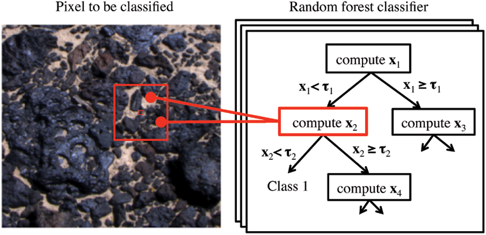
Pixel classification algorithm concept. (Color images available online at www.liebertonline.com/ast)

Each tree finds a different solution. The majority classification from all trees forms the overall class prediction. Additionally, pixel posterior class distributions are stored at each leaf, so that the system can produce posterior classification probabilities P(y|x). This indicates the system's confidence in the classification result and can be used to exclude low-confidence or ambiguous regions. It can also flag anomalous areas that are different from materials seen in the training data (Foil et al., 2013).

The training procedure requires an analyst to supply labeled data in the form of designated image regions for each class. One strategy is to use an image editing program to “paint” over the pixels, where different colors signify different surface classes. It is not necessary that the entire image be labeled; usually a few representative exemplars are sufficient, and the entire process requires just a few minutes. We can duplicate the training images and labels using different rotational transformations to grow the training set and improve the invariance of the result to orientation. Then, an automated decision forest learning procedure assigns a subset of training pixels to each decision tree and grows each tree from the root down. At each iteration, the training procedure defines the test at each node to be the one which splits the remaining data set into the most well-separated populations, with respect to the pixel labels. The specific splitting criterion we employed maximizes information gain with respect to the posterior class distribution. In this study, we used a single labeled image in our training episodes, thus demonstrating the performance of the algorithm with a small training set.

The random forest model has several beneficial properties. First, each tree's calculation is independent, so the algorithm is highly scalable and degrades gracefully with the number of trees and the number of nodes per tree. This provides a convenient means for designers to trade between execution speed and accuracy. Second, each tree requires just a few arithmetic operations, so the algorithm can be made quite fast. Third, training the trees on separate random subsets of the data promotes good generalization performance, because it avoids the idiosyncrasies of any single subset. We did not experience any problems with local minima, and classifier performance was robust across a wide range of training parameters. For further details on the forest training process, we refer the reader to previous work on decision trees (Breiman, 2001; Shotton et al., 2008; Wagstaff et al., 2013).

2.2. Instrument architecture

The physical system instantiates this algorithm in a hardware test bed capable of real-time automatic surface mapping. The TextureCam instrument consists of three main components: the cameras, the data processing unit (DPU), and a computer (Fig. 2). The cameras and the computer are unmodified commercial products, while the DPU is based on a commercial field programmable gate array (FPGA) development board with custom-built interface electronics and packaging.

FIG. 2.

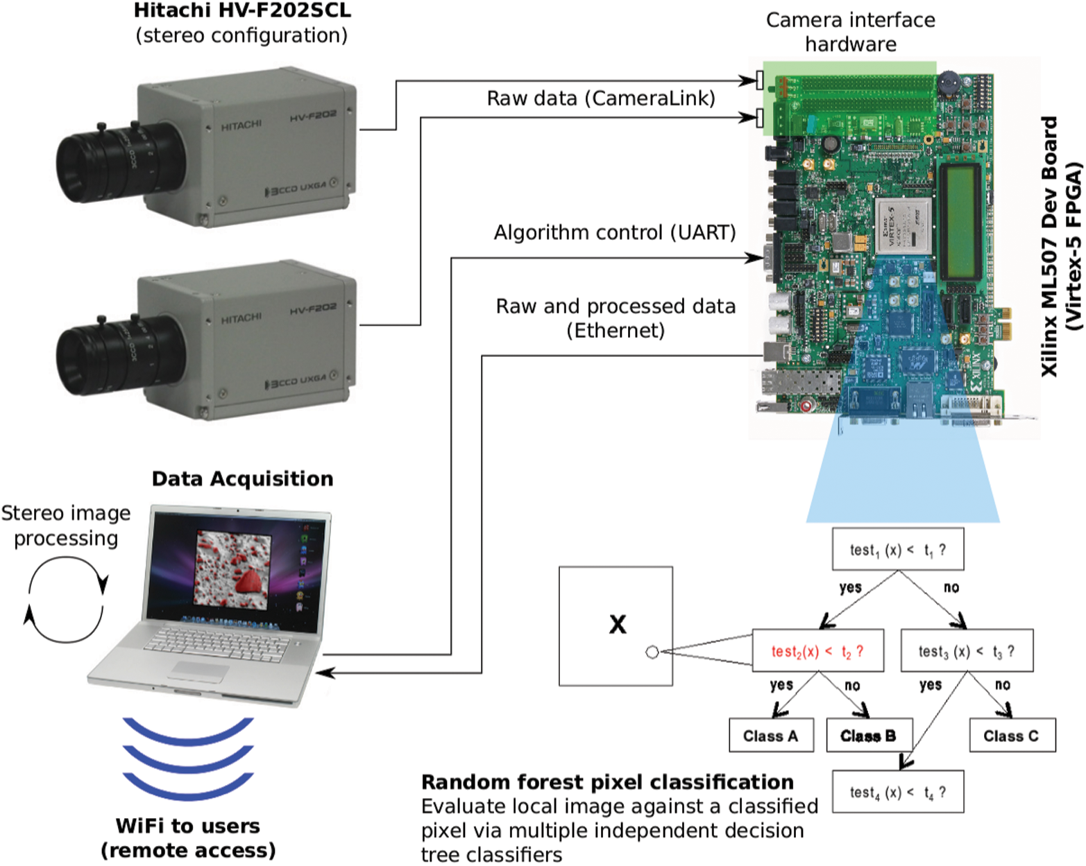
TextureCam instrument concept. During the 2013 field test, we used only one camera; the second camera (for stereo vision) will be integrated for our next field test in 2014. (Color images available online at www.liebertonline.com/ast)

We use two 3CCD Hitachi HV-F202SCL color cameras (the second camera will be integrated in the future). Each camera has three internal image sensors with filters for measuring red, green, and blue wavelengths. This configuration results in images with better precision than cameras in a 1CCD configuration, as each pixel is a true sense of its corresponding primary color. The high-fidelity images ensure that the algorithm receives a very accurate representation of the scene to be classified. In contrast, a 1CCD camera has a single image detector with, for example, a Bayer mosaic filter. Images recorded in this configuration need to be passed through a demosaicing algorithm to extrapolate the red, green, and blue values. The spectral response of the Bayer mosaic filter typically shows greater overlap in the color bands, resulting in more cross talk between the pixels and a lower dynamic range than a 3CCD camera (Fig. 3).

FIG. 3.

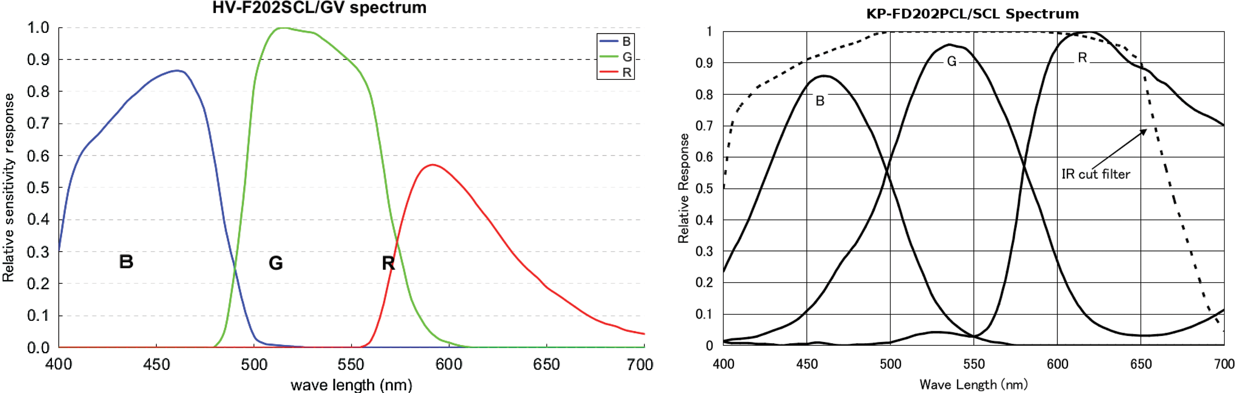
Spectral response of the Hitachi 3CCD HV-F202SCL camera (left) as compared to a similar 1CCD camera, the KP-FD202SCL (right). The individual color bands have sharper cutoffs in the 3CCD configuration (Hitachi, 2013). (Color graphics available online at www.liebertonline.com/ast)

The cameras connect to the DPU via a Mini Camera Link interface, a high-speed, serialized, low-voltage differential signaling standard commonly used in machine vision applications. This interface adapter is attached to a Xilinx ML507 FPGA development board. The data acquisition logic, the command/control of the cameras, and the random forest classifier are implemented on a Virtex-5 FPGA1. Our initial prototype performs the classification with an embedded Power-PC processor (inside the FPGA), but the random forest is well suited for an efficient logic-only implementation, since it is highly parallelizable: each pixel can be classified independently of all others in the image. Time-sensitive portions of the algorithm will be ported to the FPGA logic for the next field test. The goal is to achieve a classification output rate of 1 frame per second.

The output from the DPU is a data stream with both raw images and the classification results. This is sent over Ethernet as UDP packets in a direct connection to a computer that captures, displays, and stores these data. A time stamp along with GPS coordinates is also recorded. While the first field test only utilized one camera, the next expedition will add a second camera and stereo image processing (performed on the computer). A Wi-Fi network is used to connect field users to the computer in order to control the instrument, view raw and processed data, as well as perform training for new classifiers. This multiuser collaborative environment proved to be very efficient in our first field test.

2.3. Field mobility

We aim to evaluate this system in a range of analog field environments, which demands a portable, rugged, and fully self-sufficient prototype. For ease in transportation and for increased field mobility, the instrument is mounted on a pair of hard-frame backpacks (Fig. 4). One backpack holds a gasoline generator that provides power for all the electronics and user laptops. The other backpack holds the DPU, computer, cabling, cameras, and spare gasoline canisters. Once a field site is selected, the backpacks are placed on the ground, the generator activated, connections are made to the instrument, and the camera is placed on a tripod. The whole process takes about 5 min. An aluminum shield with a solar-powered fan protects the camera from overheating in direct sunlight, and an umbrella provides a fashionable dust cover and shade for the instrument electronics.

FIG. 4.

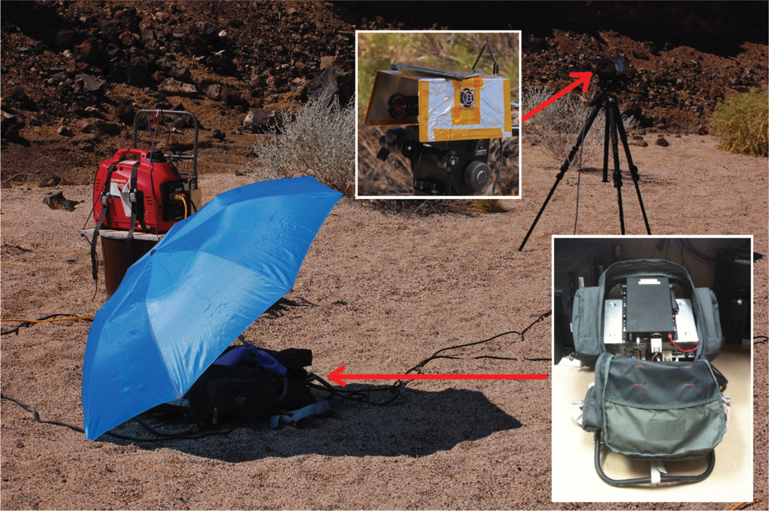
The TextureCam single-camera field instrument consists of a tripod-mounted camera with sunshade (upper inset) and a backpack-mounted DPU and control computer (lower inset). (Color images available online at www.liebertonline.com/ast)

2.4. User interface

All control of the TextureCam instrument is handled via a graphical user interface running on the computer and visible to all field users over a Wi-Fi network connection (Fig. 5). The interface allows the user to select which classifier to use from a set of classifiers preloaded on a memory card in the DPU. Commanding the instrument to acquire an image instructs the DPU to record a snapshot from the cameras, run the classifier on the raw image, and send the raw and processed image to the computer, which displays them in the user interface window. The computer (CPU) also runs the classification processing on the received raw image, allowing for an immediate visual comparison between CPU processing and FPGA processing. The “Save” command instructs the DPU to transmit the probability maps and the computer to save acquired (and self-processed) image data, as well as to record the time stamp and GPS coordinates of the current location. The temperature of the DPU and the computer is also displayed, prompting the user to shut down the instrument if operating conditions become too hot for the electronics.

FIG. 5.

The instrument is controlled through a graphical user interface over a wireless connection. The top row in the interface shows the raw image from the cameras looking at a striped training target. The bottom row shows the CPU-processed result (left) and FPGA-processed result (right). The system recognizes the striped texture of the training target, with warmer colors corresponding to a higher probability for that class. A control bar, with buttons and indicators for temperature and GPS coordinates, is present at the bottom of the frame. (Color images available online at www.liebertonline.com/ast)

3. Field Experiment Methods

We deployed our instrument prototype on a field expedition in the second year of the project. While the algorithm development and the bulk of the algorithm refinement occurred in a laboratory setting (with artificial geological and lighting conditions), there was no better test of performance and operational logistics than in a relevant environment as may be seen on a future planetary rover. We have identified a number of implementation bugs and design improvements that would have been hard to uncover in the laboratory.

3.1. Site

Our field tests took place at the southern edge of the Cima Volcanic Field (Fig. 6). This field is composed of a series of basaltic lava flows that lie in the Mojave Desert region of Southern California, ranging in age from Late Miocene (6–7 Ma) in the north to Late Pleistocene (20–500 ka) in the south (Dohrenwend et al., 1984; Wilshire, 1992; Wells et al., 1995). This entire region, averaging less than 1.5 cm of precipitation a year, has been declared a Mars analog site by the Terrestrial Analogs Panel of the National Science Foundation–sponsored Decadal Survey (Farr, 2004). More specifically, Cima was selected for this particular study due to the great diversity of surfaces observed in these volcanics, including not only textures relevant to basaltic rocks but also those applicable to unconsolidated regolith and stratified sediments (Wells et al., 1985; McFadden et al., 1987). Individual field experiments to evaluate the real-time performance of the system were designed for the following locations: (A) a highly eroded wash containing a north-facing wall that exposes multiple volcanic events interbedded with immature paleosol layers (Fig. 7) and (B) the upper surface of a volcanic lava flow that has developed a mature desert pavement interspersed with patches of clay and loose volcanic clasts (Fig. 8). The two sites were labeled Site A and Site B, respectively. The field experiment took place from April 29 to May 2, 2013, under clear skies and good midday illumination.

FIG. 6.

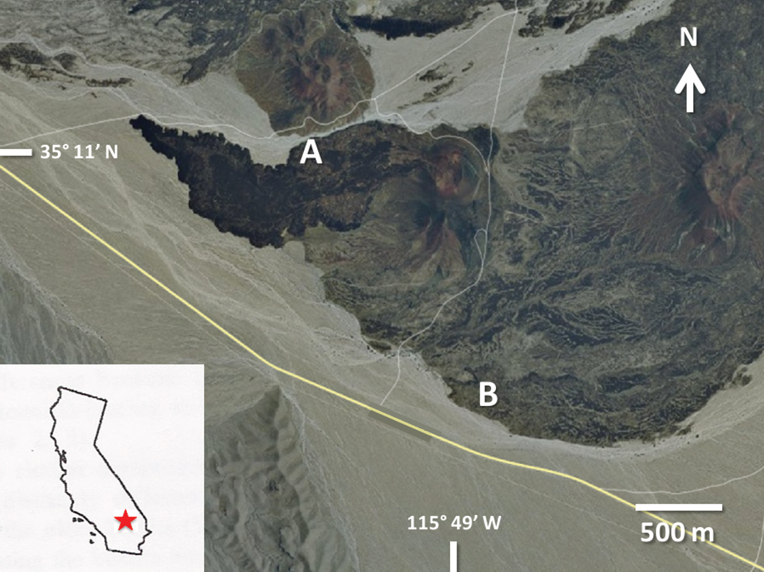
Southern edge of the Cima Volcanic Field. Located ∼25 km east-southeast of Baker, CA, in the Mojave National Preserve. Individual experiments were performed at (A) a north-facing wall, cut by erosion, exposing multiple volcanic layers, and (B) the upper surface of the southern-most lava flow. Image modified after MapQuest. (Color graphics available online at www.liebertonline.com/ast)

FIG. 7.

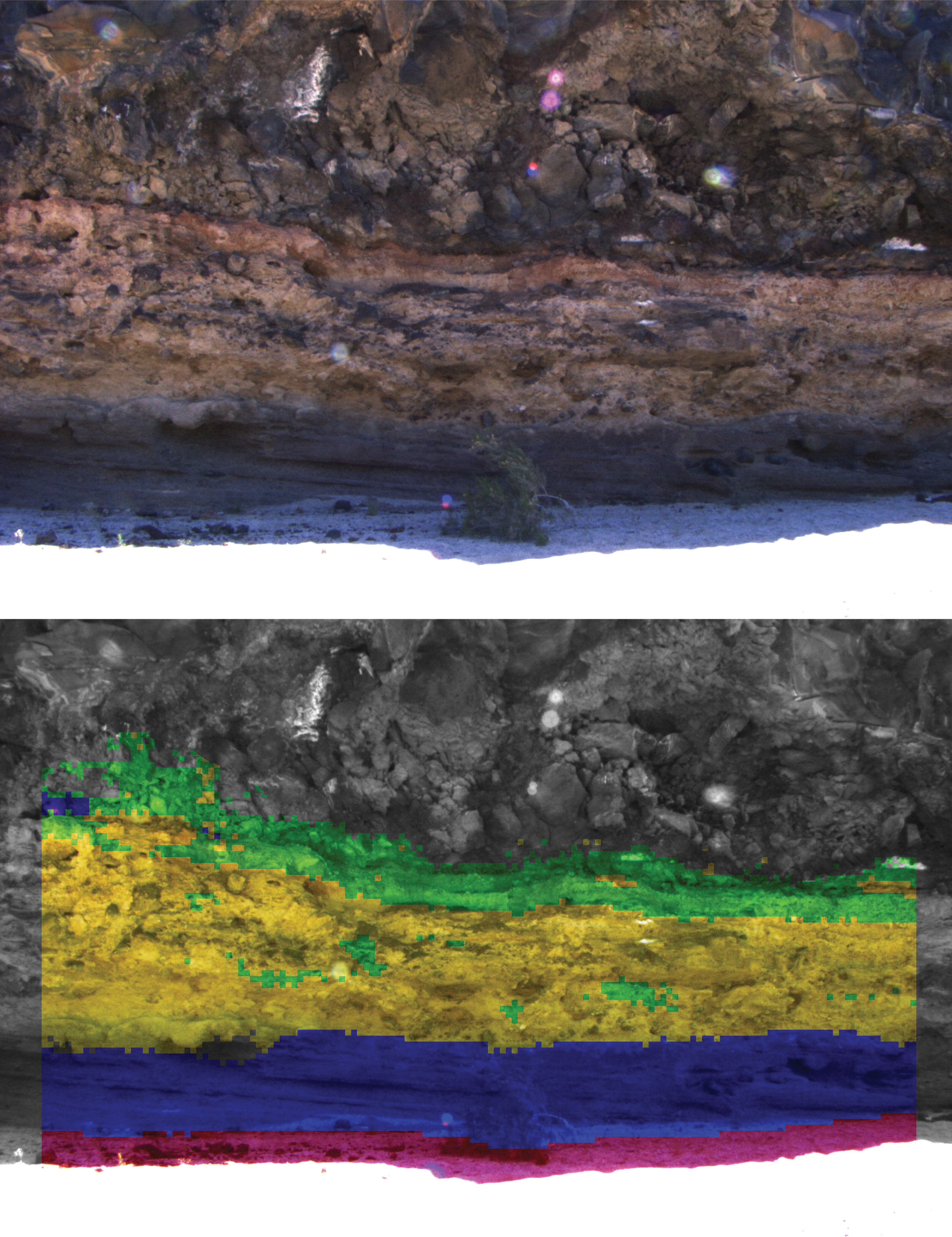
Layered units at Site A. I: Channel bed. II: Sorted volcanic gravel and lava bombs. III: Volcanic angular gravel and blocks in poorly sorted clay matrix. IV: Oxidized clay. V: Massive volcanic blocks. (Color images available online at www.liebertonline.com/ast)

FIG. 8.

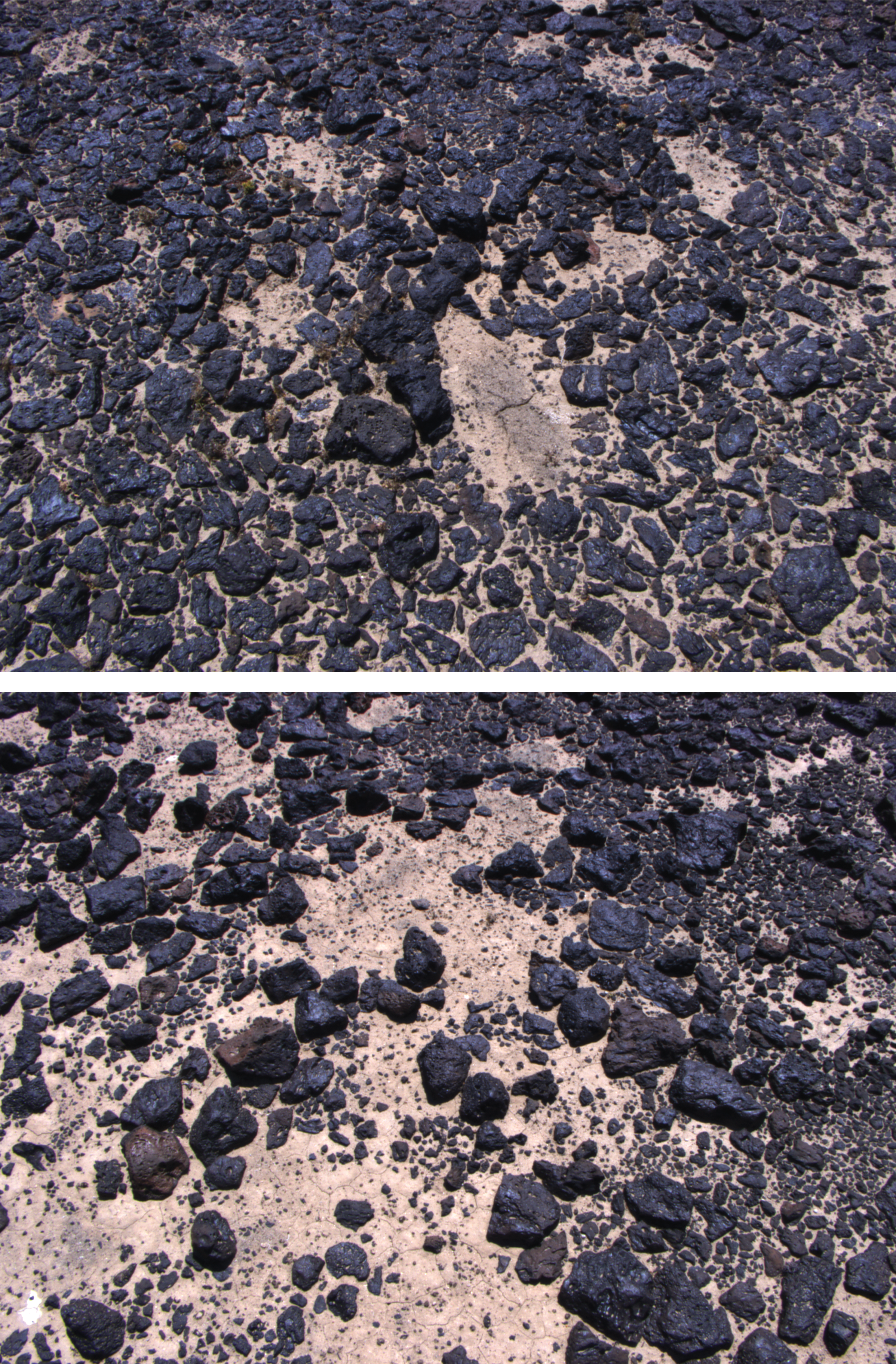
Surfaces at Site B. I: Gravel and small clasts (<64 mm in size). II: Clay sediment. III: Basalt cobbles. IV: Basalt cobbles with iron oxide coating. (Color images available online at www.liebertonline.com/ast)

We defined visually distinct textural classes in each scene. Site A exhibited at least five distinct layers (Fig. 7): (A-I) the channel bed, consisting primarily of bright sand; (A-II) a layer of volcanic angular gravel, well sorted and punctuated by locally embedded lava bombs; (A-III) poorly sorted, angular volcanic gravel, including boulder-sized clasts, suspended in a clay matrix; (A-IV) a thin and somewhat intermittent layer of red oxidized clay; and (A-V) a layer of massive basalt material. We also delineated several visually distinctive surface classes at Site B: (B-I) regions with predominant gravel-sized particles (<64 mm in size), including local patches of desert pavement; (B-II) surface covered by clay sediment; (B-III) basalt cobbles (>64 mm in size); and (B-IV) basalt cobbles with a red oxidized surface indicating differential weathering or exposure to moisture.

3.2. Data acquisition

We began each session by acquiring a single three-channel image and manually labeling examples of different classes in an image editing application (Fig. 9). This process produced a map of integer values delineating classified and unclassified areas. We then trained the random forest on a field laptop computer, building the decision tree from these training examples. This process typically required 10–15 min, with the majority of the time used for manual image labeling. At the end of the training process, we uploaded the resulting random forest definition to a flash memory card and inserted it into the instrument; all subsequent classifications used this trained model. Contrary to some previous studies (Peralta et al., 2008), we did not experience significant problems from changing light conditions, and a single training session typically provided consistent performance for the remainder of the trial. That we experienced fewer illumination issues is understandable, since our study differed from the Calderón work in several significant ways. First, the Calderón study was conducted near the winter solstice, with very low and fast-changing light angles. In contrast, we operated at favorable times of the day when the light remained relatively constant for the targets during acquisition of both training and test images. Second, that previous work focused on the problem of tracking individual features by using Scale-Invariant Feature Transform (SIFT) descriptors, a challenging problem that relies on perfect matches from one scene to the next. Tracking a specific feature is an all-or-nothing problem, and a changing shadow can cause a lost track that cannot be recovered thereafter. SIFT matching is known to be somewhat sensitive to lighting changes (Bauer et al., 2007). Finally, we provided some additional illumination invariance by preprocessing each image and converting it to a Hue Saturation Value (HSV) color representation.

FIG. 9.

(Top left, Top right) Training labels for Site B. Here, we trained the classifier using a single image. Red: B-I gravel (<64 mm). Blue: B-II sediment. Green: B-III basalt cobbles. Yellow: B-IV basalt cobbles with iron oxide coating. (Bottom right) The inferred probability map for surface class B-IV, basalt cobbles with iron oxide coatings, produced automatically by the model after training. Higher intensity corresponds to a higher probability that the surface belongs to the iron oxide class. (Color images available online at www.liebertonline.com/ast)

After training, we acquired a sequence of images to cover the area of interest. For Site A, we began approximately 12 m from the exposed wall, with the camera at 0 degrees elevation (i.e., pointed at the horizon). We collected a single training example from the extreme right side of the outcrop. We then panned the camera leftward, collecting a sequence of four images of the entire visible face of the wall and forming a mock rover panorama spanning approximately 120 degrees of azimuth. At Site B, we began with a training image with the tripod-mounted camera pointed down at approximately −45 degree elevation, observing a patch of terrain approximately 1 m wide. We then moved the camera to the transect location, where we acquired a sequence of 16 images at 1 m intervals with the camera facing the direction of motion. All image processing occurred on board the instrument; images were also saved to the instrument computer for later analysis.

We evaluated the system's performance by comparing the automatic classifications to ground truth classifications made by a human. We generated these ground truth labels in the same fashion as the training data, by manually labeling all regions of the test images according to their surface type. Ambiguous areas that could be reasonably classified as more than one class were left unlabeled and excluded from the analysis.

The classification maps would reflect any spatial correlations in the different terrain types. We quantified the degree of spatial correlation by calculating the fractional coverage of each class over the foreground of the transect images. Looking at just the foreground ensures that the areas analyzed do not overlap from one frame to the next. If the terrain types were not spatially correlated, the resulting coverage fractions would be independent and identically distributed for each class. We test this for each terrain type by treating the coverage fraction as a time series and applying a Durbin-Watson test (Durbin and Watson, 1971). This is a test for no autocorrelation based on the residuals from a regression analysis. We favor the test for its simplicity, though it does not explicitly account for the constraint that the mixing ratios must sum to one. There exist Bayesian alternatives, such as hidden state time series representations, but inference in such models can be challenging. Thus, we will favor the simpler Durbin-Watson test here. Gravel and clast coverage has been found to be similar across larger spatially extended units (Wells et al., 1985); therefore we expect these classes to fail the no-autocorrelation test. The spatial distribution of iron oxide weathering is less clear in visual inspection. Consequently, we do not have any prior expectation for that result.

4. Field Experiment Results

We first consider results at Site A. Figure 10 shows a typical classification result after each surface class has been assigned a different color. The system correctly interprets this scene as having contiguous horizontal layers. There is some slight mixing between iron oxide and clay classes, but the border of the sorted gravel layer is well localized. For clarity, we have removed classification labels above the iron oxide layer and below the channel bed. The massive basalt class (A-V) was never classified accurately (for reasons that we will discuss below); after initial attempts to retrieve it, we finally excluded it from our analysis.

FIG. 10.

Example of automatic image classification (Site A). Magenta: A-I Channel bed. Blue: A-II Sorted volcanic gravel. Yellow: B-III Volcanic angular gravel and blocks in clay matrix. Green: A-IV Oxidized clay. Class A-V (massive volcanic blocks) is excluded. (Color images available online at www.liebertonline.com/ast)

In Fig. 11, performance is quantified at Site A with a receiver operating characteristic (ROC) curve. The ROC curve treats each class as a one-versus-many classification problem, showing true-positive and false-positive rates that can be achieved for different probability thresholds. The operator can modify acceptance thresholds to move along this curve; for example, one can reduce the number of false positives by requiring classifications to be very certain. However, this will find fewer examples of each class. Conversely, lower probability thresholds result in more false positives. The ROC curve characterizes this tradeoff. Curves in the upper left of the plot suggest powerful classifiers with desirable performance profiles. These curves were produced by averaging the ROC performance from all images in the data set.

FIG. 11.

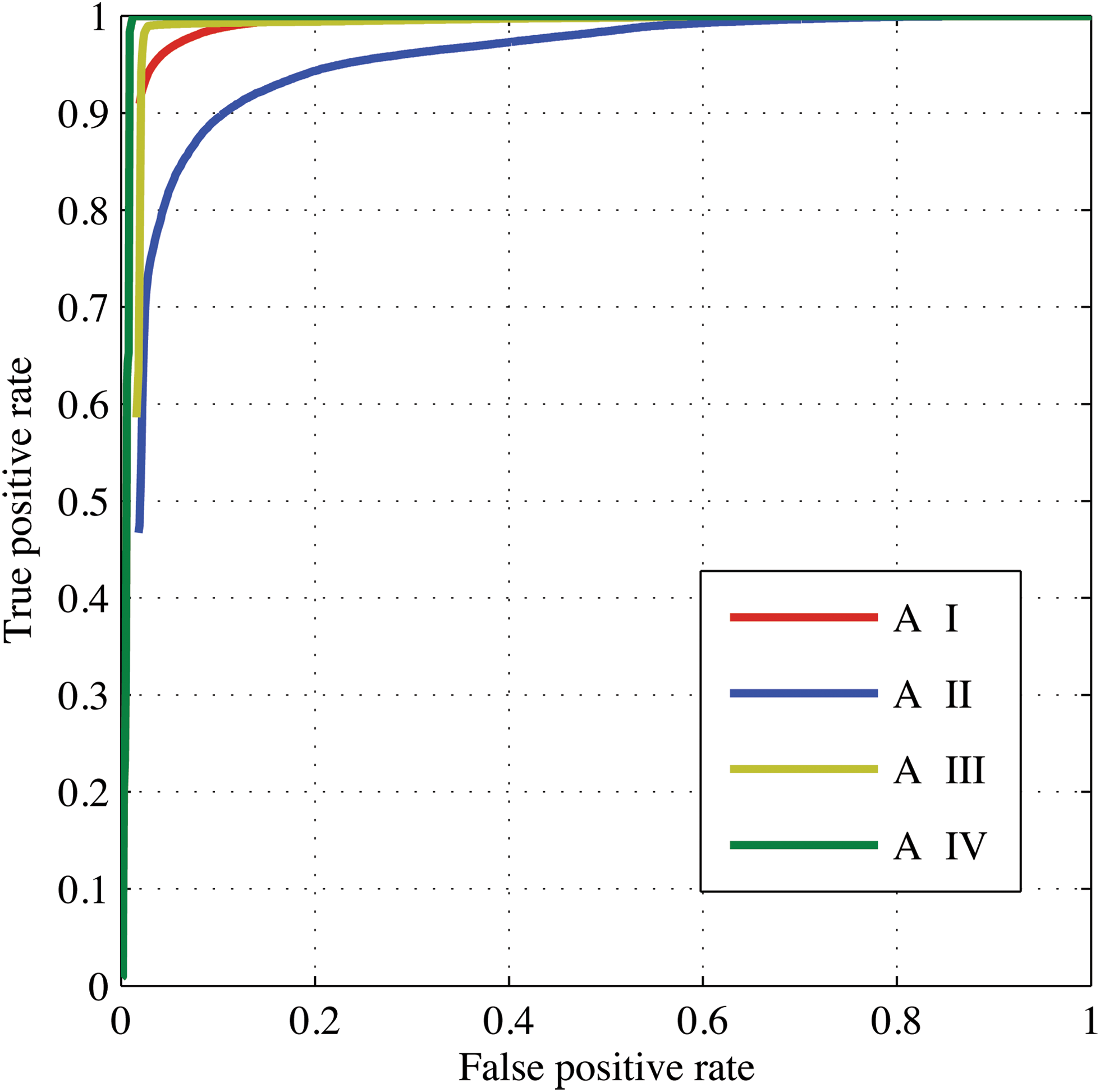
ROC curve for Site A. The upper left corner represents ideal performance, detecting 100% of true positives with no false alarms. (Color graphics available online at www.liebertonline.com/ast)

The ROC curve for site A shows near-perfect performance on three of five classes; the system recovers 90% of classes A-I, A-III, and A-IV with negligible false positives. We are mainly interested in the leftmost portion of the ROC curve, since this is appropriate for a rover that collects just a few follow-up observations of high-probability targets. The performance demonstrated at Site A would allow a rover to perform representative sampling—a single follow-up measurement of each surface—with very high confidence. Class A-II is the most difficult, and the rate of false positives becomes non-negligible if one wishes to capture the entire surface, as the dark gravel area grades into the shadowed sediment directly below it. Table 1 shows confusion matrices calculated over all pixels in the data set. This also shows some shadow-induced confusion between sediment and gravel classes. We have normalized each entry, dividing by the number of true examples of that class. Thus, the rows of the confusion matrices sum to one, but the columns in general do not.

Table 1.

Confusion Matrix for Classes at Site A

	Predicted
	A-I	A-II	A-III	A-IV
Actual
A-I Sediment	0.796	0.204	0.000	0.000
A-II Gravel	0.031	0.965	0.004	0.000
A-III Clay matrix	0.000	0.000	0.982	0.018
A-IV Iron oxide	0.000	0.000	0.003	0.997

Bold entries show the precision of each automatic class label, for example, the fraction that is correctly assigned.

Figure 12 provides a typical classification result for Site B, which captures both the size and distribution of rocks as well as the presence or absence of iron oxide coatings. Figure 13 shows the ROC curve calculated over all images at Site B. The system is highly effective at mapping the fundamental basalt/sediment distinction but less accurate for the iron oxide and gravel classes. Again, this level of accuracy is sufficient for representative sampling because it is possible to select high-probability pixels that guarantee a negligible false-positive rate. Table 2 shows a confusion matrix. Overall performance is good, but there are some classes that are occasionally confused. For instance, the distinction between gravel and cobbles is less obvious in the upper portion of the images, since the camera sees little of the sediment substrate at extreme aspect ratios.

FIG. 12.

Example of Cima image classification (Site B). Red: B-I gravel (<64 mm). Blue: B-II sediment. Green: B-III basalt cobbles. Yellow: B-IV basalt cobbles with iron oxide coating. (Color images available online at www.liebertonline.com/ast)

FIG. 13.

ROC curve for Site B. The best performance is in the upper left corner. (Color graphics available online at www.liebertonline.com/ast)

Table 2.

Confusion Matrix for Classes at Site B

	Predicted
	B-I	B-II	B-III	B-IV
Actual
B-I Basalt gravel	0.807	0.182	0.010	0.001
B-II Sediment	0.005	0.993	0.001	0.001
B-III Basalt cobbles	0.023	0.013	0.961	0.003
B-IV Iron oxide	0.000	0.516	0.005	0.479

Bold entries show the precision of each automatic class label.

However, most mislabelings represent the intrinsic subjectivity of the classes at Site B rather than difficulty in recognizing visual appearance. The distinction between sediment with small, sparsely scattered rocks and the gravel is somewhat blurred. Often isolated gravel particles are justifiably counted as belonging to the surrounding sediment unit. The iron oxide class performs worst, with approximately half the area labeled as basalt cobbles. This also reflects some inherent subjectivity, since the two are simply end members of a distribution of coatings with different degrees of weathering and iron oxide coatings. The fact that approximately half these pixels are mislabeled is compatible with the good precision evidenced in the ROC curve; there are many fewer iron oxide pixels than basalt, so a large proportion of them can be ignored without significantly increasing the overall false-positive rate. That places some rare iron oxide within the more mundane background class, which is not a problem for rovers attempting to use this information for instrument targeting—operators can use a high-probability threshold to ensure any iron oxide pixels they do select are likely to be real.

Table 3 shows the fractional coverage of each terrain type for the 16 images in the Cima sequence, and the p value of the Durbin-Watson test for no autocorrelation of the time series. Low p values for the sediment, basalt, and gravel class suggest that these three units are not uncorrelated. This is appropriate because these three classes represent spatially extended phenomena on meter scales, while the iron oxide class represents an anomalous weathering condition that occurs intermittently on the surfaces of individual rocks. Figure 14 displays the same information as a bar chart. Figure 15 shows two extreme examples from the sequence: Image 2 (left), which is estimated to have the smallest fraction of sediment, and Image 12 (right), which has the largest. We conclude that spatial trends in the mapped sequence are consistent with the mesoscale spatial correlations expected for these terrain types.

FIG. 14.

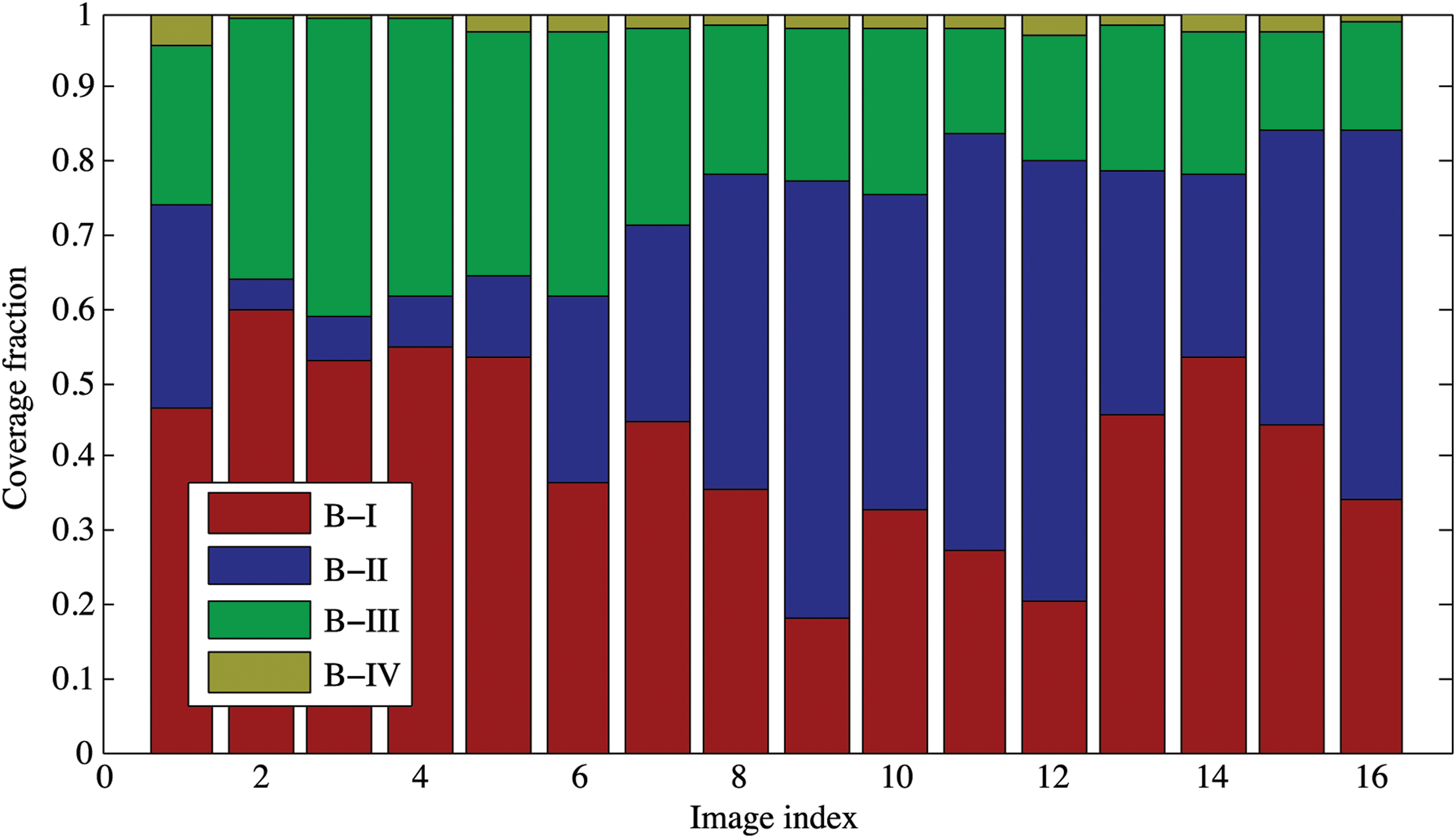
Coverage fractions for each terrain type, for each image in the site B traverse sequence. (Color graphics available online at www.liebertonline.com/ast)

FIG. 15.

Transect image 2, classified as having the smallest sediment fraction (Top) and transect image 12, having the largest fractional area of estimated sediment (Bottom). (Color images available online at www.liebertonline.com/ast)

Table 3.

Fractional Coverage of Each Surface Type in Each Transect Image, and p Values of a Durbin-Watson Test for Autocorrelation in Each Class

Image	B-I	B-II	B-III	B-IV
1	0.47	0.27	0.21	0.05
2	0.60	0.04	0.35	0.01
3	0.53	0.06	0.41	0.01
4	0.55	0.07	0.38	0.01
5	0.54	0.11	0.33	0.02
6	0.37	0.25	0.36	0.02
7	0.45	0.26	0.27	0.02
8	0.35	0.43	0.20	0.01
9	0.18	0.59	0.21	0.02
10	0.33	0.43	0.22	0.02
11	0.27	0.56	0.14	0.02
12	0.20	0.60	0.17	0.03
13	0.46	0.33	0.20	0.02
14	0.53	0.25	0.19	0.03
15	0.44	0.40	0.13	0.03
16	0.34	0.50	0.15	0.01
p value	0.011	0.002	0.008	0.240

5. Discussion

The experiments described above represent a challenging test of automated geologic image analysis. They evaluated the instrument in true field conditions with just a single training episode and no effort made to retune instrument parameters on the fly. These tests involved large contiguous mosaics of both vertical and horizontal surfaces, both with and without obvious stratigraphy. To our knowledge, it is the first time automated geologic image analysis of this kind has been demonstrated in real-time instrument hardware. We will continue to refine the instrument, methods, and training sets, but this work provides an initial test of system performance and a bound on the errors that can be expected in an operational setting.

The overall result is encouraging, though we found a wide variation in mapping accuracy across different surface types. Certain distinctions were quite simple to teach the classifier, such as the difference between differently colored volcanic strata (Site A) or the obvious visual distinction between sediment and rock (Site B). Accuracy rates for pure, unambiguous classes are typically above 95%, which represents a high likelihood of acquiring good targeted data regardless of the class abundance. This level of performance is already sufficient to improve rover exploration efficiency over status quo methods; rock detection is important for instrument targeting (Estlin et al., 2012), while layer detection is useful for a range of instrument placement and mapping operations (Gulick et al., 2001; Wagstaff et al., 2013). In some cases, the automatic classification outperformed the initial human labeling, as in the iron oxide class at Site A. Here, small image regions labeled as iron oxide led to the discovery of isolated patches of this class outside the main layer.

These tests also hint at more challenging classes, which may benefit from special preprocessing or postprocessing. For example, the massive block class (A-V) is visually distinctive when looking at the entire rock face, but the instrument must make a classification decision based only on the local information near each pixel. Local surface textures provided insufficient information to reliably delineate the class. The iron oxide coatings on rocks at Site B are another challenging scenario. These targets were small and scattered, so that a labeling that did not correctly identify the perimeter of each iron oxide surface would incur a high penalty in terms of total pixel area. Even with this caveat, instrument targeting with these classifications would significantly outperform blind targeting when the features at a new locale are not known in advance. But the performance variation by class means that operators seeking maximum reliability should define the desired targeting behavior in terms of simple and localized visual patterns.

The rare classes highlight the related and important issue of class imbalance. Our baseline classifier does not typically take the relative abundance of each class into account, but the true probability may shift as the predominance of classes changes. This is easy to remedy; in the case of class imbalance one could apply an additional informed prior P(y) using Bayes' rule. This would amount to scaling each output probability by the relative abundance of each class. A similar scaling can capture different misclassification costs, leading to a Bayes' optimal classification with maximum total utility. By applying these simple postprocessing operations, a single generic random forest could be applied for many different scenarios.

6. Future Work

There are two principal avenues for future work: algorithm improvements and hardware integration. We plan to improve classification performance using more sophisticated preprocessing and a richer set of pixel attributes. Local descriptors (Dalal and Triggs, 2005) or oriented bar filters (Wagstaff et al., 2013) could improve performance, though their computational expense would probably demand specialized hardware support. We will also consider ways to address the challenge of spatial context, evidenced in class A-V where nonlocal information is required. Candidate solutions include input attributes that capture a larger spatial context or class prior probabilities based on image location (Crandall et al., 2005).

We are also investigating further hardware upgrades in preparation for our next field expedition scheduled for summer 2014. We are currently adding the second Hitachi camera and porting the algorithm into the FPGA fabric. The addition of the second camera will enable stereo vision processing on the computer. The resulting range estimates will be used to select appropriate classifiers for each part of the scene. In porting the algorithm from the embedded PowerPC processor inside the FPGA to the surrounding fabric, we hope to achieve a 1 Hz processing rate by performing multiple per-pixel decision-tree evaluations in parallel. We will also make the instrument more convenient to use by extending the Wi-Fi range and reducing Ethernet data drops.

7. Conclusions

This work provides several unique new contributions to the field. First, we have taken random forest algorithms recently demonstrated for Mars surface geology (Wagstaff et al., 2013) and applied them to real-time geologic surface analysis in a field environment. This demonstrates that the same basic algorithm applies to both scenarios and suggests a potential for a wide range of different rover science autonomy tasks. Unlike previous tests, which have generally relied on traditional computing platforms, we have implemented our classifier system directly in embedded instrument hardware. The resulting system was evaluated at two distinct regions in the Cima Volcanic Fields, where it successfully classified visually distinctive surface patterns by using color and texture cues. Further work will continue to refine preprocessing, the algorithm itself, and the instrument platform.

Footnotes

Acknowledgments

The TextureCam project is supported by the NASA Astrobiology Science and Technology Instrument Development program (NNH10ZDA001N-ASTID) and National Park Service permit MOJA-2013-SCI-0011. Accommodations for the field experiment were provided by the Desert Studies Center, Zzyzx, CA, a field station of the California State University (CSU).

This work was carried out at the Jet Propulsion Laboratory, California Institute of Technology, under a contract with the National Aeronautics and Space Administration. Government sponsorship acknowledged.

Abbreviations

DPU, data processing unit; FPGA, field programmable gate array; ROC, receiver operating characteristic; SIFT, Scale-Invariant Feature Transform.

References

Bakambu

J.N.

, Langley

, Pushpanathan

, MacLean

W.J.

, Mukherji

, and Dupuis

(2012) Field trial results of planetary rover visual motion estimation in Mars analogue terrain. Journal of Field Robotics, 29:413–425.

Bauer

, Sunderhauf

, and Protzel

(2007) Comparing several implementations of two recently published feature detectors. In Proceedings of the International Conference on Intelligent and Autonomous Systems, Vol. 6, IAV, Toulouse, France.

Breiman

(2001) Random forests. Machine Learning, 45:5–32.

Crandall

, Felzenszwalb

, and Huttenlocher

(2005) Spatial priors for part-based recognition using statistical models. In IEEE Computer Society Conference on Computer Vision and Pattern Recognition, Vol. 1, Institute of Electrical and Electronics Engineers (IEEE), Piscataway, NJ, pp 10–17, doi:10.1109/CVPR.2005.329.

Dalal

and Triggs

(2005) Histograms of oriented gradients for human detection. In IEEE Computer Society Conference on Computer Vision and Pattern Recognition, Vol. 1, Institute of Electrical and Electronics Engineers (IEEE), Piscataway, NJ, pp 886–893, doi:10.1109/CVPR.2005.177.

Deans

, Lees

, Smith

, Cohen

, Morse

, and Fong

(2012) Field testing next-generation ground data systems for future missions [abstract 2518]. In 43^rd Lunar and Planetary Science Conference Abstracts, Lunar and Planetary Institute, Houston.

Dohrenwend

J.C.

, McFadden

L.D.

, Turrin

B.D.

, and Wells

S.G.

(1984) K-Ar dating of the Cima volcanic field, eastern Mojave Desert, California: Late Cenozoic volcanic history and landscape evolution. Geology, 12:163–167.

Durbin

and Watson

G.S.

(1971) Testing for serial correlation in least squares regression. Biometrika, 58:1–19.

Estlin

T.A.

, Bornstein

B.J.

, Gaines

D.M.

, Anderson

R.C.

, Thompson

D.R.

, Burl

, Castaño

, and Judd

(2012) AEGIS automated science targeting for the MER Opportunity rover. ACM Trans Intell Syst Technol, 3:50:1–50:19.

10.

Farr

T.G.

(2004) Terrestrial analogs to Mars: the NRC community decadal report. Planet Space Sci, 52:3–10.

11.

Foil

, Thompson

D.R.

, Abbey

, and Wettergreen

(2013) Probabilistic surface classification for rover instrument targeting. In IEEE/RSJ International Conference on Intelligent Robotic Systems, Institute of Electrical and Electronics Engineers (IEEE), Piscataway, NJ, pp 775–782, doi:10.1109/IROS.2013.6696439.

12.

Francis

, McIsaac

, Thompson

D.R.

, and Osinski

G.R.

(2014) Autonomous rock outcrop segmentation as a tool for science and exploration tasks in surface missions. In Proceedings of SpaceOps, Pasadena, California.

13.

Furgale

and Barfoot

T.D.

(2010) Visual teach and repeat for long-range rover autonomy. Journal of Field Robotics, 27:534–560.

14.

Grotzinger

, Crisp

, Vasavada

, Anderson

, Baker

, Barry

, Blake

, Conrad

, Edgett

, Ferdowski

, Gellert

, Gilbert

, Golombek

, Gómez-Elvira

, Hassler

, Jandura

, Litvak

, Mahaffy

, Maki

, Meyer

, Malin

, Mitrofanov

, Simmonds

, Vaniman

, Welch

, and Wiens

(2012) Mars Science Laboratory mission and science investigation. Space Sci Rev, 170:5–56.

15.

Gulick

V.C.

, Morris

R.L.

, Ruzon

M.A.

, and Roush

T.L.

(2001) Autonomous image analyses during the 1999 Marsokhod rover field test. J Geophys Res, 106:7745–7764.

16.

Hitachi (2013) HV-F202SCL/GV, KP-FD202PCL/SCL Specifications, Hitachi, Ltd., Japan. Available online at http://www.hitachikokusai.com.

17.

McFadden

, Wells

, and Jercinovich

(1987) Influences of eolian and pedogenic processes on the origin and evolution of dsert pavements. Geology, 15:504–508.

18.

McGuire

P.C.

, Gross

, Wendt

, Bonnici

, Souza-Egipsy

, Ormö

, Díaz-Martínez

, Foing

, Bose

, Walter

, Oesker

, Ontrup

, Haschke

, and Ritter

(2010) The cyborg astrobiologist: testing a novelty detection algorithm on two mobile exploration systems at Rivas Vaciamadrid in Spain and at the Mars Desert Research Station in Utah. International Journal of Astrobiology, 9:11–27.

19.

Mlynarczuk

, Górszczyk

, and Slipek

(2013) The application of pattern recognition in the automatic classification of microscopic rock images. Comput Geosci, 60:126–133.

20.

Mustard

J.F.

, Adler

, Allwood

, Bass

D.S.

, Beaty

D.W.

, Bell

J.F.

III , Brinckerhoff

W.B.

, Carr

, Des Marais

D.J.

, Drake

, Edgett

K.S.

, Eigenbrode

, Elkins-Tanton

L.T.

, Grant

J.A.

, Milkovich

S.M.

, Ming

, Moore

, Murchie

, Onstott

T.C.

, Ruff

S.W.

, Sephton

M.A.

, Steele

, and Treiman

(2013) Report of the Mars 2020 Science Definition Team, white paper posted July 2013 by the Mars Exploration Program Analysis Group (MEPAG). Avilable online at http://mepag.jpl.nasa.gov/reports/MEP/Mars_2020_SDT_Report_Final.pdf.

21.

Peralta

F.C.

, Thompson

D.R.

, and Wettergreen

(2008) Autonomous rover reflectance spectroscopy with dozens of targets. In International Symposium on Artificial Intelligence, Robotics and Automation in Space (ISAIRAS), February 26–29, Hollywood, CA.

22.

Shotton

, Johnson

, and Cipolla

(2008) Semantic texton forests for image categorization and segmentation. In IEEE Conference on Computer Vision and Pattern Recognition, 2008, Institute of Electrical and Electronics Engineers (IEEE), Piscataway, NJ, pp 1–8, doi:10.1109/CVPR.2008.4587503.

23.

Squyres

S.W.

, Arvidson

R.E.

, Baumgartner

E.T.

, Bell

J.F.

III , Christensen

P.R.

, Gorevan

, Herkenhoff

K.E.

, Klingelhöfer

, Madsen

M.B.

, Morris

R.V.

, Rieder

, and Romero

R.A.

(2003) Athena Mars rover science investigation. J Geophys Res Planets, 108, doi:10.1029/2003JE002121.

24.

Thompson

D.R.

, Smith

, and Wettergreen

(2008) Information-optimal selective data return for autonomous rover traverse science and survey. In IEEE International Conference on Robotics and Automation, 2008, Institute of Electrical and Electronics Engineers (IEEE), Piscataway, NJ, pp 968–973, doi:10.1109/ROBOT.2008.4543330.

25.

Thompson

D.R.

, Wettergreen

, and Peralta

F.J.C.

(2011) Autonomous science during large-scale robotic survey. Journal of Field Robotics, 28:542–564.

26.

Wagstaff

, Castano

, Dolinar

, Klimesh

, and Mukai

(2004) Science-based region-of-interest image compression [abstract 1934]. In 35^th Lunar and Planetary Science Conference Abstracts, Lunar and Planetary Institute, Houston.

27.

Wagstaff

K.L.

, Thompson

D.R.

, Abbey

, Allwood

, Bekker

D.L.

, Cabrol

N.A.

, Fuchs

, and Ortega

(2013) Smart, texture-sensitive instrument classification for in situ rock and layer analysis. Geophys Res Lett, 40:4188–4193.

28.

Wells

, Dohrenwend

, McFadden

, Turrin

, and Mahrer

(1985) Late Cenozoic landscape evolution on lava flow surfaces of the Cima volcanic field, Mojave Desert, California. GSA Bulletin, 96:1518–1529.

29.

Wells

S.G.

, McFadden

L.D.

, Poths

, and Olinger

C.T.

(1995) Cosmogenic ³He surface-exposure dating of stone pavements: implications for landscape evolution in deserts. Geology, 23:613–616.

30.

Wilshire

H.G.

(1992) Geologic Map of the Indian Spring Quadrangle, San Bernardino County, California, Open-File Report 92-181, U.S. Geological Survey, Denver, CO.

31.

Woods

, Shaw

, Barnes

, Price

, Long

, and Pullan

(2009) Autonomous science for an Exomars rover–like mission. Journal of Field Robotics, 26:358–390.

32.

Woods

, Shaw

, and Rendell

(2011) High-level autonomy and image prioritisation for long distance Mars rovers. In Proceedings of the 11^th Symposium on Advanced Space Technologies in Robotics and Automation, ESTEC, Noordwijk, the Netherlands, pp 12–14.