Extending Galactic Habitable Zone Modeling to Include the Emergence of Intelligent Life

2.1. Monte Carlo habitability model

The starting point for the present study was the model of the Milky Way developed by Gowanlock et al. (2011). In that model, various major observable properties of the disk of the Milky Way were used to populate stars and planets on an individual basis using Monte Carlo methods. To assess habitability, they modeled SNe as a function of the properties of the Milky Way, planet formation, and the time required for the emergence of complex life. Their modeling of the galactic disk incorporates a total stellar mass, an initial mass function (IMF), a three-dimensional stellar number density distribution, a star formation history, and a galactic chemical evolution model. They only consider disk stars with galactocentric radii greater than 2.5 kpc, because of difficulties in accurately modeling the region inside 2.5 kpc due to the complicated formation history of the bulge. Nevertheless, their model includes ∼75% of the disk stars in the Galaxy, where the disk contains the majority of the stars in the Milky Way. Four variants of the model were proposed to assess sensitivity to variations in the parameters outlined above. In particular, two IMFs were utilized [Kroupa (2001) and Salpeter (1955)] and two stellar number density distributions [Jurić et al. (2008) and Carroll and Ostlie (2006)]. A fixed total disk mass (Binney and Tremaine, 2008), star formation history, and associated galactic chemical evolution model (Naab and Ostriker, 2006) were employed.

All the models explored by Gowanlock et al. (2011) reproduced the same general behavior and found that habitability was the greatest toward the inner Galaxy. In the present study, we concentrate only on the most pessimistic model (Model 4), based on a Kroupa IMF and found to have 1.2% of all stars hosting a habitable planet (of which 0.9% are tidally locked and 0.3% are nonlocked to their host stars). For a detailed definition of the model and its associated parameters, see the work of Gowanlock et al. (2011).

Transient radiation events in the Milky Way create cosmic rays, X-rays, and gamma rays, which can deplete planetary atmospheres of ozone, expose planets to their host stars, and thus cause massive extinctions to land-based life [see Melott and Thomas (2011) for an overview of radiation hazards to our biosphere]. The Gowanlock et al. (2011) model focuses on the ability of planets to survive SN sterilizations. Given a total disk mass, an IMF, stellar number density distribution, and star formation history, type II supernovae (SNII) and type Ia supernovae (SNIa) were populated independently, which expresses differences in formation rates and sterilization distances between these types of SNe. It was assumed that planets nearby these SNe (the sterilization distances of which reflect distributions of absolute magnitudes of observations) will be uninhabitable for a finite time period after a sterilization event occurs, and the planet can recover from the event.

Supernovae occur throughout the Milky Way, and there is even evidence of them occurring in recent geological history. Benítez et al. (2002) suggested that ∼2 Myr ago a SN caused significant damage to Earth's ozone layer, which had an effect on the extinction of ocean life at the Pliocene-Pleistocene boundary. Furthermore, Bishop and Egli (2011) suggested that ∼2.8 Myr ago Earth was nearby a SN, as evidenced by ⁶⁰Fe in deep-sea crust. In line with Gowanlock et al. (2011), we focus on SNe, which we assume to be the dominant danger to habitability.

Gowanlock et al. (2011) found that the highest density of habitable planets occurs in the regions with the highest stellar densities and consequently highest frequency of SN events. As with other previous works on the habitability of galaxies (Lineweaver et al., 2004; Prantzos, 2008; Carigi et al., 2013), they did not account for stellar kinematics such as radial mixing, or oscillations above and below the midplane that may lead to varying levels of exposure to cosmic rays (Medvedev and Melott, 2007), on the basis that such motions were expected to have an insignificant overall negative impact on the fraction of habitable planets. Gowanlock et al. (2011) did not find a region in the Milky Way that was continuously sterilized or sterilized at a sufficiently high frequency that planetary systems traveling through such a region would have a high probability of becoming sterilized. Should such a region have existed, then incorporating stellar motions above and below the midplane would have a greater impact on the results. Note that a star above or below the midplane that passes through it would be entering a region where there is a higher density of habitable planets (and hence cannot be significantly more hazardous to habitability). Therefore, oscillations above and below the midplane are unlikely to significantly decrease habitability, especially since oscillations of this type result in those stars still spending the majority of their time above or below the midplane. If such vertical stellar oscillations had been considered in Gowanlock et al. (2011), the mixing would have produced a degree of averaging in the results for habitability above and below the midplane, slightly weakening the observed trends.

Gowanlock et al. (2011) populated the stars in their model by assigning each one a birth date, main sequence lifetime, and metallicity from the galactic chemical evolution model and star formation history, which assumes an inside-out formation history of the Milky Way. The metallicity-planet correlation of Fischer and Valenti (2005) was used, in combination with the population synthesis models of Ida and Lin (2005), to assign habitable planets to host stars in the model.

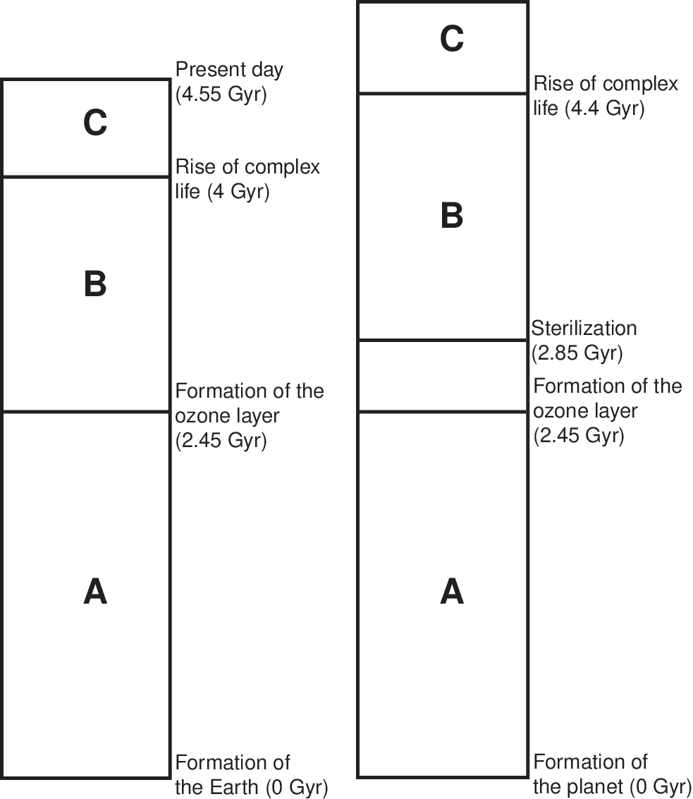
The timescales in Earth's history were adopted to calculate whether a planet is habitable. This is arguably the most speculative assumption in the model, as there is only Earth's pathway to complex (and intelligent) life to suggest such conditions on other planets. In light of focusing on dangers caused by SN events to planetary biospheres and, in particular, atmospheric ozone depletion, the focus is on the timescales for the buildup of ozone on Earth. The notion of planetary oxygenation time is adopted from the work of Catling et al. (2005), which proposes that, on Earth, a continuous duration of oxygenation is required for the emergence of complex life. Gowanlock et al. (2011) assumed that (1) any sterilizations that occur on the planets populated in the model before the ozone layer forms (this was approximately 2.3 Gyr ago on Earth) have no effect on habitability (since any life at this stage is assumed not to be surface-dwelling) and (2) the emergence of complex life requires a sufficient time period isolated from sterilization events to allow for sufficient oxygenation for the emergence of complex life. Therefore, if a SN occurs within a threshold distance of d pc between the time period that the ozone formed and the period afterward that is required for the emergence of complex life, then this has a resetting effect, and the planet must remain unsterilized for a time period before it is considered habitable.

Gowanlock et al. (2011) used the work of Gehrels et al. (2003), who found that a SNII will deplete the ozone layer and have a sterilizing effect on planets at a distance of <8 pc. The 8 pc distance was assumed to be just sufficient to sterilize a planet. By using the absolute magnitudes of SNII and SNIa events, a distribution of sterilization distances was developed to reflect the notion that different magnitude events can occur and lead to varying sterilization distances.

For SNII, d was selected from a probability distribution within the range of ∼2–27 pc, and within the range of ∼14–27 pc for SNIa. Figure 1 shows an illustration of the timescales that demonstrate the interrelationship between sterilizations and the major events in Earth's history used to calculate the habitability of a planet in the model of Gowanlock et al. (2011). Note that region C in Fig. 1—the time after a planet becomes habitable—is the focus of the present work in extending the modeling to include the evolution from complex to intelligent life.

OPEN IN VIEWER

FIG. 1.

Left: Illustration of the major timescales on Earth used as criteria to calculate the habitability of a planet. For a given planet in our model, we assume that a sterilization occurring before the formation of the ozone layer has no effect (A), whereas a sterilization occurring during the period of continuous oxygenation does have an effect (B), and C shows the time since the rise of complex life to the present day. Right: Employing the timescales from Earth (on the left), we illustrate the effect a sterilization has on a planet populated in our model. A sterilization in A has no effect, since the ozone layer has not yet formed. However, the sterilization in B, shown at 2.85 Gyr, delays the possibility of complex life until 4.4 Gyr, as it disrupts the requirement of continuous oxygenation time. The time period C shows a hypothetical duration in which complex life has not been affected by any sterilization events after the planet is considered habitable at 4.4 Gyr.

2.2. Gap time analysis

The methodology described above for assessing habitability is based on identifying planets that provide conditions conducive to the evolution of complex land-based animal life. We assume that this represents the starting point for further stages of evolution that could lead to the emergence of intelligent life and, beyond that, to technological civilizations. In assessing the propensity for complex life to further evolve to intelligent life, φ _I, our fundamental assumption is that time is the primary barrier to this process. We reason that environmental conditions, at least at the beginning of the process, are favorable, given that they were deemed suitable for complex life to develop. We then consider the time period beyond that needed for the appearance of complex life to see whether sufficient time is available for further evolution to intelligence. We assume that this process would be disrupted by any nearby SNe; that is, if a SN occurs before intelligence is reached, the process is reset. The time durations between such SNe are referred to as gap times, and we assume φ _I is strongly dependent on the number and length of these gap times. Without proposing a specific relationship between gap time length and its effect on φ _I, we suggest it is a reasonable assumption that longer gap times will provide greater opportunity for the emergence of intelligence.

Our analysis of gap times follows essentially the same methodology as employed by Gowanlock et al. (2011) but with an extended parameter range for the time duration between SNe. The goal was to assess whether these additional time requirements for the evolution of intelligence would alter the basic findings of Gowanlock et al. (2011), that is, to investigate the extent to which the regions of greatest propensity for intelligence corresponded to regions of greatest habitability (as defined for complex life). On Earth, the evolution from complex life to intelligence took just under 0.6 Gyr. Rather than apply this single figure, we acknowledge the lack of understanding of how the process works (and hence how long it typically takes) by considering a range of durations. As will be explained in Section 2.3, our metrics are based on cumulative gap times conditioned on a variable threshold value ranging from 0 to 2 Gyr. We prefer this approach over assigning a specific probability distribution to the time required for intelligence to emerge for two reasons: (1) we have insufficient data to meaningfully ascribe a shape or mean value to this distribution, and (2) there are potential sensitivities that may be revealed by our model that could be masked by the averaging effect of applying a distribution.

At this point, it is important to note that, if a planet is assessed as “habitable,” it does not mean that it will definitely become inhabited by complex life—only that conditions are favorable for this to happen. Likewise, if there is a long gap time between SNe on a habitable planet, it is not assured that intelligent life will emerge—only that this becomes a possibility. In this work, we do not attempt to quantify the percentage of planets that give rise to intelligence. We seek to produce a metric for φ _I that allows analysis of the relative likelihood of intelligence emerging in different regions and epochs of the Galaxy. A conservative position would be to assume that complex or intelligent life may only be able to arise on a small fraction of habitable planets. The opposite position would be that it is likely to arise on the majority of habitable planets. Either assumption, or any in between, can be made without affecting the veracity of any conclusions drawn from analyzing relative propensities.

Figure 2 illustrates how gap times are related to the major events in a planet's timeline. For the illustrative example given, there are three gap times, labeled GAP₁, GAP₂, and GAP₃. GAP₁ is the time from the formation of a complete ozone layer to the first of two SNe, SN₁. GAP₂ is the time between SN₁ and SN₂. GAP₃ is the time from SN₂ to the present (or equally, death) time of the example planet. For the emergence of complex land-based animal life, we assume the same timeframe as observed on Earth, that is, 1.55 Gyr. Where a gap time exceeds 1.55 Gyr, this provides an opportunity for further evolution to intelligent life. In the example of Fig. 2, there are two such opportunity times, T _O, which we may calculate as T _On =(GAP _n – 1.55) when GAP _n ≥1.55, and zero otherwise. Since GAP₂ is less than 1.55 Gyr, there is assumed to be no opportunity for the emergence of complex or intelligent life during that interval, hence T _O2=0.

OPEN IN VIEWER

FIG. 2.

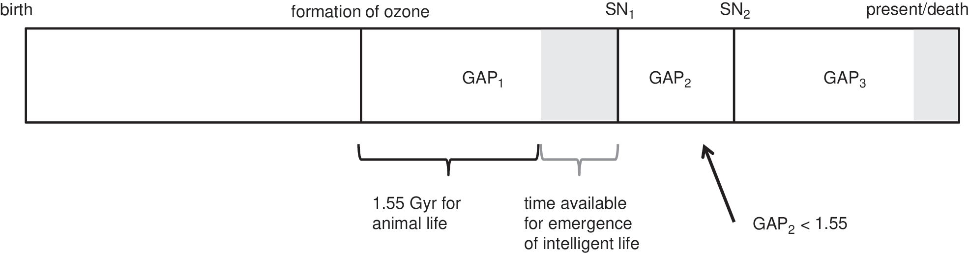
Illustrative planet timeline showing the major events from the birth (at left) to the present (or death) time (at right) and showing how “gap times” are calculated. In this example, there are two SNe, labeled SN₁ and SN₂. A gap time begins after the first formation of the ozone layer or after a SN event. A gap time is ended by a SN, the death of the planet, or the present day, as we do not extrapolate beyond the age of the Universe. Any gap times exceeding 1.55 Gyr (the time assumed to be needed for the emergence of animal life) give rise to an opportunity for intelligent life to emerge. The shaded regions represent these “opportunity times,” T _O, which are equal to the gap time less 1.55 Gyr.

The Monte Carlo simulation described in Section 2.1 provides a hypothetical population of planets, along with pertinent data for each planet, including its location coordinates, birth/death dates, and a list of dates the planet was sterilized by SNe. Locations are specified by x, y, and z coordinates relative to the galactic center, as shown in Fig. 3. The x and y coordinates define the position projected onto the galactic midplane, and z is the height above (when positive) or below (when negative) the midplane. The galactocentric radius, r, is given by (x ²+y ²)^1/2. We elected to work with a subset of the entire galactic data set to take advantage of azimuthal symmetry, specifically a 15° sector of the full 360° data set, as illustrated in Fig. 3. Even with this fraction, our model included in excess of 70 million planets, which is sufficient to allow statistical sampling errors to be ignored and to safely assume that the chosen 15° sector would produce the same results as any other 15° sector. The metrics generated from this data set (as described in Section 2.3) were scaled by a factor of (360/15) to obtain results that represent the entire Galaxy.

OPEN IN VIEWER

FIG. 3.

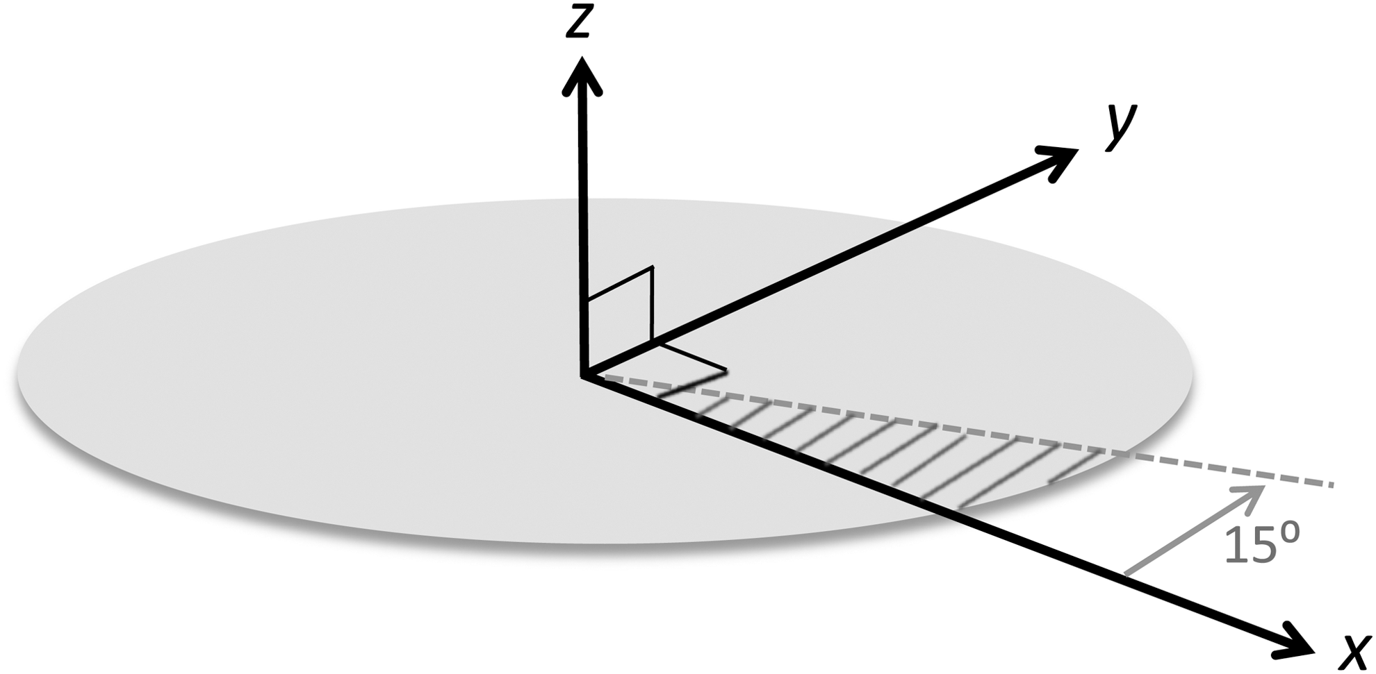
The coordinate system employed in the simulation model of Gowanlock et al. (2011) for defining planet locations relative to the galactic center at (x, y, z)=(0, 0, 0). The model generates data for the entire 360° of “azimuth” in the (x, y) plane. To simplify processing for the present study, only a 15° subset was analyzed, exploiting the model's azimuthal symmetry.

From the planet data set, one can assess which planets are habitable [according to the criteria set by Gowanlock et al. (2011)] and additionally calculate the gap times experienced on each habitable planet. For some planets, no gaps exceeding 1.55 Gyr occur; for others, one or more such gaps occur. We treat multiple gaps on a single planet in an equivalent way to single gaps on multiple planets, that is, as independent opportunities for life to evolve. The total number and length of all gap times for all habitable planets produced by the simulation are accumulated, binned according to spatial location and temporal epoch, from which further analysis can be conducted.

2.3. Propensity metric

We are primarily interested in examining how the propensity for the emergence of intelligent life, φ _I, varies as a function of spatial location and epoch within the Galaxy. To investigate this, we create a metric for φ _I and observe, for our simulated planet population, the variability of this metric over time and as a function of r and z.

A straightforward metric, which we term φ _Iu, is the accumulated sum of all opportunity times, T _On , for the planets existing within a specified spatial bin. (For a single planet, this would correspond to summing the lengths of time represented by the gray shaded regions in Fig. 2.) That is, \documentclass{aastex}\usepackage{amsbsy}\usepackage{amsfonts}\usepackage{amssymb}\usepackage{bm}\usepackage{mathrsfs}\usepackage{pifont}\usepackage{stmaryrd}\usepackage{textcomp}\usepackage{portland, xspace}\usepackage{amsmath, amsxtra}\pagestyle{empty}\DeclareMathSizes{10}{9}{7}{6}\begin{document} \begin{align*}\varphi_{\rm Iu} (r_j) = \mathop\sum_n T_{{\rm O}n}\end{align*} \end{document}

where r_j is the center value of the j ^th spatial bin. For example, if the data are binned according to galactocentric radius using bins of width w, then the radius range corresponding to r_j is [(r_j - w/2)≤r<(r_j +w/2)].

This method of computing φ _Iu is equivalent to assuming a uniform probability distribution for the required time for intelligent life to emerge. That is, the required time is assumed to be a uniformly distributed random variable; hence the total probability will be proportional to the total cumulative time.

A variation for computing φ _Iu involves setting a threshold time, T _thresh, for the T _O values, and only those T _O≥T _thresh are included in the summation. For example, the rise of animal life on Earth occurred when the planet was ∼4 Gyr old, and it was a further ∼0.6 Gyr for the rise of intelligent life. If we assume these timescales, that is, that 0.6 Gyr is the minimum time for intelligence to emerge after a planet can support complex life, then only those T _O≥0.6 Gyr are included in the summation.

We do not know the precise relationship between the value of T _O and the probability that intelligence will emerge during a time window of that length. It seems likely that the process of evolving intelligence requires a number of essential subprocesses, each occurring in sequence and each having its own specific time-distribution. This assumption was made by Carter (2008) and Forgan (2009). If this were the case, the overall time to achieve intelligence would be a random variable with a distribution approaching Gaussian (following the Central Limit Theorem) ¹ . The uniform and Gaussian models for the probability distribution of the time for evolving intelligence are illustrated in Fig. 4. Although the Gaussian model may be more appropriate than the uniform model, it has the difficulty that we do not know the scale factor on the time axis. We do not know where the mean of the distribution lies relative to the 0.6 Gyr that was required on Earth. The three example Gaussian distributions in Fig. 4 (“Gaussian a,” “Gaussian b,” and “Gaussian c”) illustrate alternative timescales. If “Gaussian a” was an accurate representation, this would suggest that intelligence arose late on Earth. Conversely, if “Gaussian c” was an accurate representation, this would suggest that intelligence arose early on Earth. Without a calibrated timescale, we cannot assess the sensitivity of φ _I to changes in T _O. For example, if typical T _O values are to the left of the Gaussian bell-curve, then a small incremental increase in T _O will result in a large increase in φ _I. However, if the T _O values are to the right of the bell-curve, then an incremental increase in T _O will have little effect on φ _I. Because of these uncertainties, there are difficulties in developing a φ _I metric that derives from a Gaussian (or any non-uniform) distribution. Furthermore, if we accept the premise that time is the primary determinant for φ _I, then a φ _I metric based on the summation of available time is not unreasonable. Therefore, we elect to employ the uniform propensity metric, φ _Iu, when generating the results reported in Sections 3.1, 3.2, and 3.3 below. Additionally, in Section 3.4, we propose an alternative method of analysis that obviates the difficulties of having to make any assumptions regarding the probability distributions for the time required for the emergence of intelligence. That methodology and its results are described in Section 3.4.

OPEN IN VIEWER

FIG. 4.

Alternative models for the probability distribution of the time taken for intelligence to evolve from animal life. The relationship between the propensity for the emergence of intelligent life, φ _I, and opportunity time T _O is dependent on this distribution. Shown are the uniform case and three different Gaussian cases of differing means relative to 0.6 Gyr (the time it took on Earth for animal life to evolve intelligence).

3.1. Propensity metric—uniform model

For the uniform model described in Section 2.3, the propensity for intelligent life is modeled as being proportional to total opportunity time, that is, the sum of all T _O≥T _thresh. Figure 5 presents the results for φ _Iu for five alternative values of T _thresh over the radius range 2.5–15 kpc. The vertical axis represents the radial density of φ _Iu, that is, φ _Iu per parsec of radius.

OPEN IN VIEWER

FIG. 5.

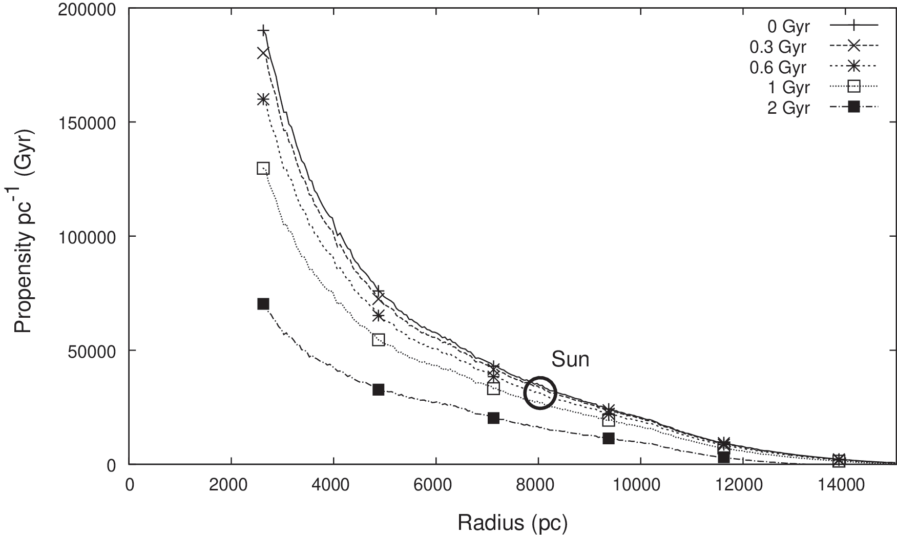
Propensity metric φ _Iu as a function of r for five time threshold values, T _thresh, ranging from 0 to 2 Gyr. The vertical axis is the radial density of φ _Iu, i.e., φ _Iu per parsec of radius. For the uniform model, φ _Iu is modeled as being proportional to total opportunity time, i.e., the sum of all T _O≥T _thresh.

The results exhibit two main features:

(1) For all values of T _thresh, φ _Iu is greatest toward the inner disk of the Galaxy; and

The first observed feature is consistent with the trends in habitable planet density reported by Gowanlock et al. (2011). To assess whether this result simply tracks the habitable planet density, we also examine the average of φ _Iu per habitable planet, which has been plotted in Fig. 6. It is seen that the average propensity does indeed vary with radius, displaying a region of maximum average propensity between about 6 and 10 kpc. At smaller radii, the average propensity is marginally lower, which can be attributed to the higher rate of SN events. At larger radii there is a rapid decline in average propensity, which can be attributed to the reducing average age of habitable planets with increasing r. This in turn is due to the later epochs at which the critical metallicity for habitable planet formation occurs with increasing r. (The variation of φ _Iu with epoch time is discussed further in Section 3.5). Despite the variations in average propensity per planet, the overall favorability of the inner Galaxy, as seen in Fig. 5, is due to the sheer number of habitable planets predicted by the model in this region.

OPEN IN VIEWER

FIG. 6.

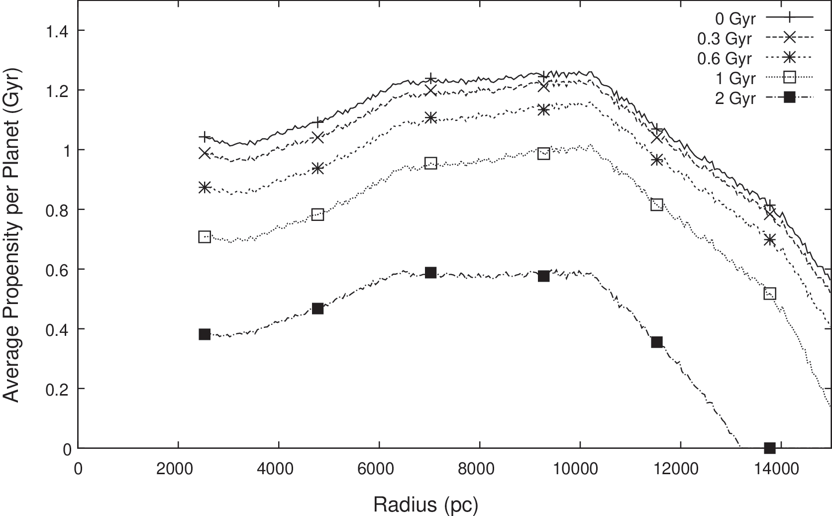
Average of φ _Iu per habitable planet as a function of r for five T _thresh values ranging from 0 to 2 Gyr. The vertical axis is the radial density of the per-planet average of φ _Iu, i.e., the average of φ _Iu per parsec of radius.

The results of Fig. 5 suggest φ _Iu will peak at some radius less than 2.5 kpc (but assumed to be greater than zero due to the proximity of the central black hole). The precise location of the peak cannot be determined, as it lies beyond the lower radius range of our model. However, the basic conclusion of the favorability of the inner Galaxy is not altered by the precise location of the peak, only the definition of “inner.” Were the model of Gowanlock et al. (2011) to be extended in future to lower radii, the analysis of this paper could be repeated to provide a closer bound on the radius of peak propensity.

The second observed feature in Fig. 5—the consistent reduction in φ _Iu with increasing T _thresh—is predictable, given that larger values of T _thresh permit fewer T _O to be included in the metric summation.

For reference, we have marked on Fig. 5 the circumstances that hold for the Sun and Earth (i.e., r=8 kpc and T _thresh=0.6 Gyr). The value of φ _Iu for these parameters is ∼35,000 Gyr per radial parsec. This is the aggregated propensity for all habitable planets occupying an annular ring of 1 pc width, at a galactocentric radius of 8 kpc (noting from Fig. 6 that the average φ _Iu per planet is ∼1.1 Gyr in this region). It is seen that for lower radii, the density of φ _Iu per radial parsec is up to 4–5 times higher. This is due to the higher number density of habitable planets in this region, rather than the average φ _Iu per planet (which we see from Fig. 6 is ∼0.9 Gyr in this region). This may be interpreted as follows: we know that intelligent life can arise (it has arisen at least once) at 8 kpc, and there should be an even greater chance that it has arisen in regions closer to the galactic center. This is seen even with larger T _thresh assumptions, up to 2 Gyr.

A different approach to examining the propensity for intelligence was taken by Forgan and Rice (2010), who used the Rare Earth hypothesis framework. They also found that the inner Galaxy should have the greatest number of intelligent civilizations. Despite major differences in model assumptions and goals between this work and theirs, the overall conclusions are in general agreement.

3.2. Propensity above and below the midplane

We now consider the variation of φ _Iu in two spatial dimensions: r and z. We present the results in the form of contour maps, which show r on the horizontal axis, z on the vertical axis, and a color-coding of φ _Iu in the plot.

Figure 7 shows the φ _Iu contour maps for five values of T _thresh, ranging from 0 to 2 Gyr. A logarithmic scale is used for the color-coding, allowing greater detail to be seen in regions where the φ _Iu values are low. Each contour map represents a cross-sectional view of the Galaxy, approximately to scale. The figure illustrates that, for T _thresh values of 0, 0.3, and 0.6 Gyr, the inner Galaxy has the highest φ _Iu at the midplane, as φ _Iu is dominated by the number of planets in the region. For these T _thresh values we see the influence of SN sterilizations between r≈5 and r≈9 kpc, where φ _Iu is slightly higher above and below the midplane at these radial positions. For T _thresh=2 Gyr, which assumes that the timescale for the rise of intelligence is more than 3 times that experienced on Earth, from 2.5 to ∼12 kpc, φ _Iu is always greater above and below the midplane.

OPEN IN VIEWER

FIG. 7.

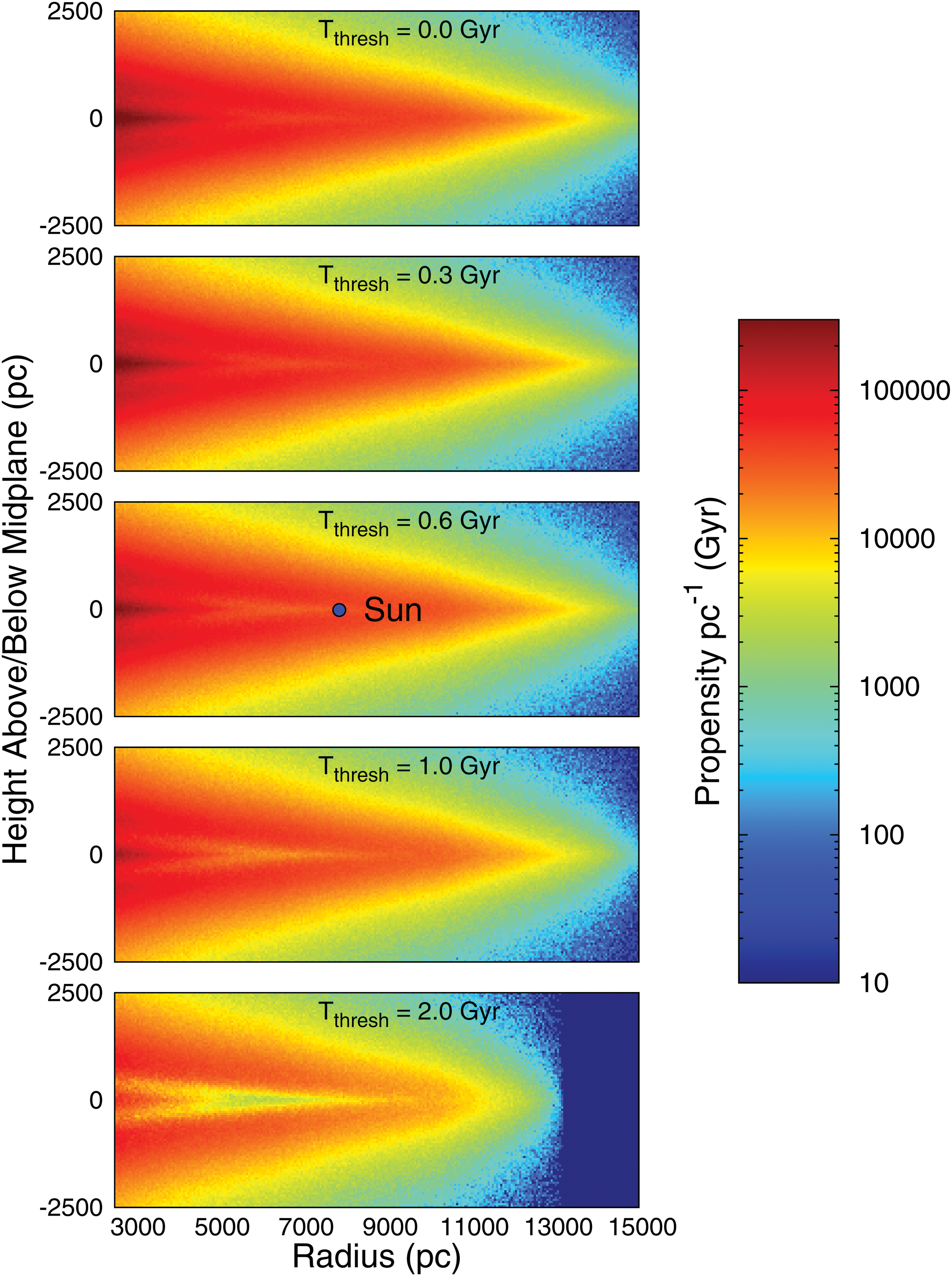
Contour map plots of φ _Iu as a function of r and z. Five separate contour maps are provided, corresponding to T _thresh values of 0, 0.3, 0.6, 1, and 2 Gyr, respectively. A logarithmic scale is used for the color-coding, which is defined in the legend given at the right. (Color graphics available at www.liebertonline.com/ast)

We know that intelligent life has arisen at least once at r=8 kpc near the galactic midplane, and there should be an even greater chance that it has arisen in those regions that are shown as “hotter” on the contour map, such as closer to the galactic center. Furthermore, if intelligence typically takes longer to arise than it has on Earth, the model suggests SETI should prioritize targets above and below the midplane at our radial position and toward the inner Galaxy. However, if intelligence takes roughly the same time as it has on Earth, or less, then the model suggests SETI should target the midplane of the inner Galaxy.

3.3. Propensity expressed in galactic coordinates

For SETI, it is instructive to consider how φ _Iu varies as a function of the pointing direction of Earth-based telescopes, specifically the variation of φ _Iu over galactic coordinates. We show this in Fig. 8, where φ _Iu (for the T _thresh=0.6 Gyr case) has been plotted as a function of galactic longitude (l) and galactic latitude (b). A logarithmic color-coding has been used to show the total φ _Iu per bin of area on the sky, where bins of approximately one square degree have been used across the whole sky ² . The three panels correspond to range limits from the observer of 3, 4, and 5 kpc, each plotted with the same color-coding range for φ _Iu. Each panel shows the entire sky in an equal-area sinusoidal projection, as seen from a vantage point of r=8 kpc and z=0, Earth's approximate location. As discussed earlier, the central bulge and inner disk (r<2.5 kpc) are excluded in our model. For this reason, results beyond a range of 5.5 kpc from the observer are incomplete with our model, which is why only ranges below 5.5 kpc have been shown.

OPEN IN VIEWER

FIG. 8.

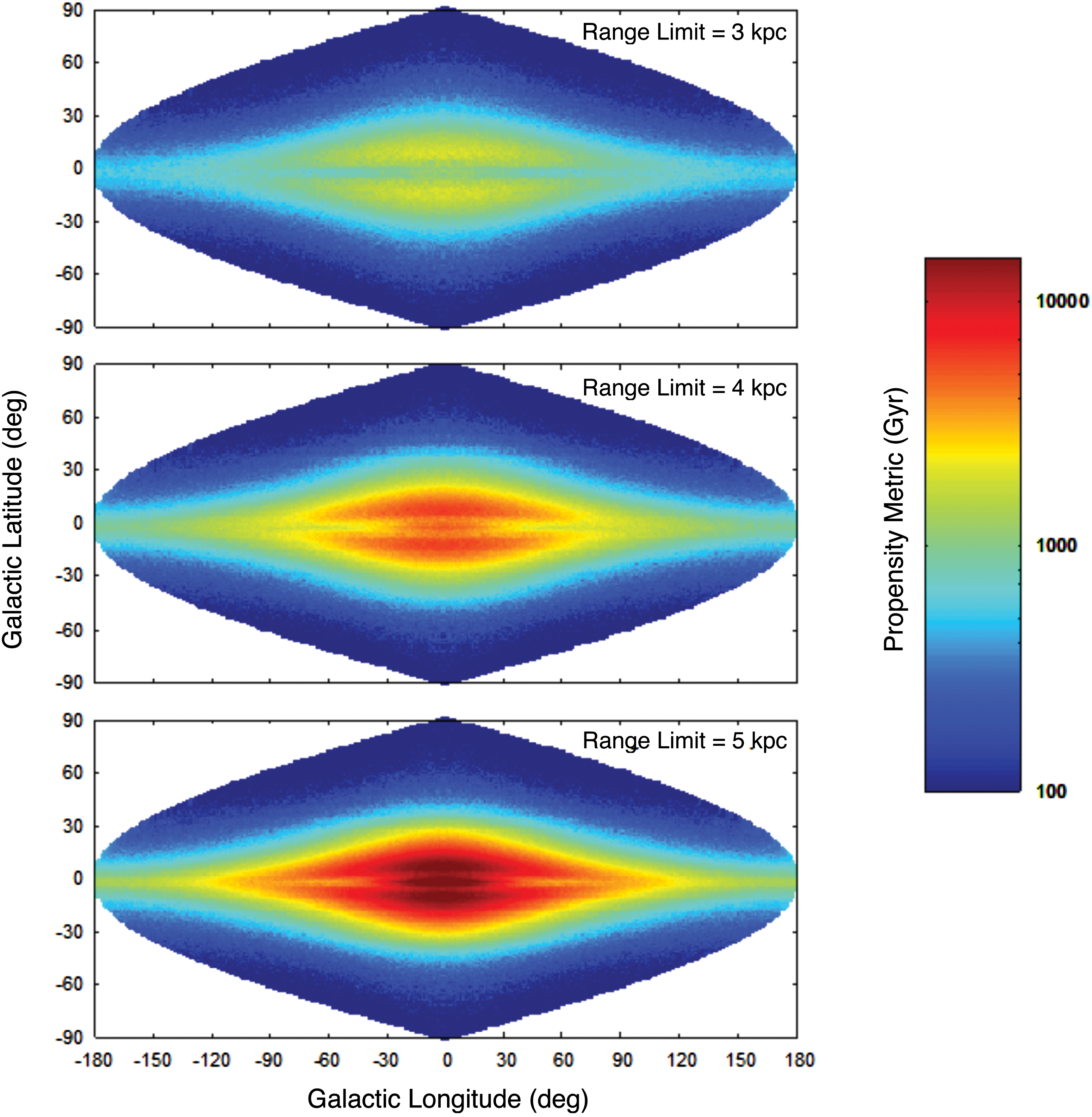
Contour map plots of φ _Iu (for T _thresh=0.6 Gyr) as a function of galactic longitude (l) and latitude (b), for three range limit cases: 3, 4, and 5 kpc. Note that the longitude scale shown applies only to b=0. The plots employ an equal-area sinusoidal projection, where the scale of the horizontal axis varies with latitude, i.e., proportionally to cos(b). (Color graphics available at www.liebertonline.com/ast)

Figure 8 can be interpreted as showing the relative density of potential targets per antenna pointing as a function of location in the sky. For a range limit of 3 kpc, the density is relatively low, because this represents a small volume of sky that contains relatively few habitable planets. Within this range, there is a minor advantage to observing toward the galactic center, and slightly above or below the midplane, consistent with our findings in Section 3.3. Increasing the range limit to 4 kpc increases the observed volume of sky and also includes more of the inner Galaxy. Consequently, the number of potential targets is significantly higher. The advantage of observing above/below the midplane remains. At a range limit of 5 kpc, the observed volume of sky is larger again and includes a significant fraction of the inner Galaxy. The density of potential targets is clearly the highest toward the inner Galaxy, in a region bounded roughly by |l|≤∼30° and |b|≤∼15°. The advantage of observing slightly above/below the midplane remains but is now less pronounced, which is consistent with the fact that more planets are now included that are closer to the galactic center, where the highest density was found to be on the midplane (see Section 3.3).

The implication of Fig. 8 for SETI is that a compelling strategy would appear to be a complete survey of a region of the sky centered on the galactic center and spanning approximately 60° of longitude and 30° of latitude. Note that the majority of target planets in this region will be close to the galactic center, so searches should focus on deliberate transmissions3.

3.4. Opportunity time distributions

Although the statistical relationship between T _O and φ _I cannot be known precisely for the reasons discussed in Section 2.3, it is still possible to make meaningful statements concerning relative propensities in our model. Across the numerous habitable planets in the model, opportunities occur of varying durations, spanning a continuum of T _O values. We create histograms of the distribution of T _O durations in Fig. 9 for seven different galactocentric radii. A radial bin size of 50 pc is used in each case, with the bin centers as listed in the figure legend.

OPEN IN VIEWER

FIG. 9.

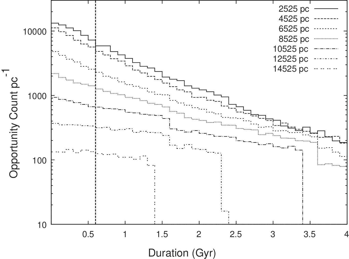
Histograms of T _O of differing durations for seven specific values of r. The vertical axis shows the number of opportunities per parsec of radius (on a logarithmic scale) that have the duration given on the horizontal axis. The dashed vertical line crossing the horizontal axis at 0.6 Gyr corresponds to the T _O experienced when intelligence arose on Earth. The cutoffs are a result of the age distribution of stars across the disk, where no planets beyond a given r can have an associated duration because they are too young.

The first feature to be noted in Fig. 9 is that shorter T _O occur more frequently than longer T _O. The maximum count occurs at the shortest durations, and the count decreases monotonically with increasing duration. This is expected, as the SN resetting events make longer durations less probable.

The second feature of Fig. 9 is that the T _O count for a given duration value tends to decrease with increasing r. This is explained by the decreasing habitable planet density with increasing r. Crucially, it is seen that the curves for each radius case do not cross, meaning that this relationship holds for all T _O durations. That is, if one considers a particular T _O duration, then regardless of the duration value, there will always be a greater number of opportunities of that duration toward the inner Galaxy. Regardless of the statistical relationship that exists between T _O and φ _I, there are always more opportunities at each duration value in the inner Galaxy, so the overall φ _I must be higher in this region.

This has neatly allowed us to circumvent the calibration issue raised in Section 2.3. We may not be able to comment meaningfully on absolute values of φ _I, but we can make the robust assertion that φ _I values are relatively higher toward the inner Galaxy. For example, with reference to Fig. 9, the opportunity count corresponding to Earth's scenario (T _O=0.6 Gyr and r=8 kpc) is ∼1500 per parsec. At lower radii, toward the inner Galaxy, the opportunity count is seen to be greater than 6000 per parsec. That is, the inner Galaxy presents more than 4 times the number of opportunities (of the duration needed on Earth for intelligence to emerge) than the region in which Earth is located. This provides further support for the conclusion drawn in Sections 3.1 and 3.2, that is, that there is a greater likelihood that intelligence will arise in the inner Galaxy than at Earth's radius.

A further observation from Fig. 9 is that, at high radii, there is a hard cutoff in the T _O distributions. Above the cutoff duration there are no opportunities for intelligence to emerge. For example, for r=14,525 pc, there are no opportunities longer than approximately 1.4 Gyr. This is due to the lower age of planets at higher radii. In the case of 14,525 pc radius, there are no planets in the model that are old enough to provide a gap between SN events greater than (1.55+1.4)=2.95 Gyr.

3.5. Opportunities by epoch

We have seen that the abundance and duration of opportunities, as encapsulated by our metric φ _Iu, varies with r and z. It is also instructive to investigate how opportunities vary by epoch, that is, as a function of time since the formation of the Galaxy. In Fig. 10, we plot total opportunity counts versus epoch time for six values of r, for the case of T _thresh=0.6 Gyr. The horizontal axis is the time since the formation of the Galaxy. At any point on the time axis, the corresponding count on the vertical axis represents the total number of habitable planets on which there is currently an “active” opportunity for intelligent life to evolve. Each opportunity contributes to the count value at all time values during the extent of the opportunity.

OPEN IN VIEWER

FIG. 10.

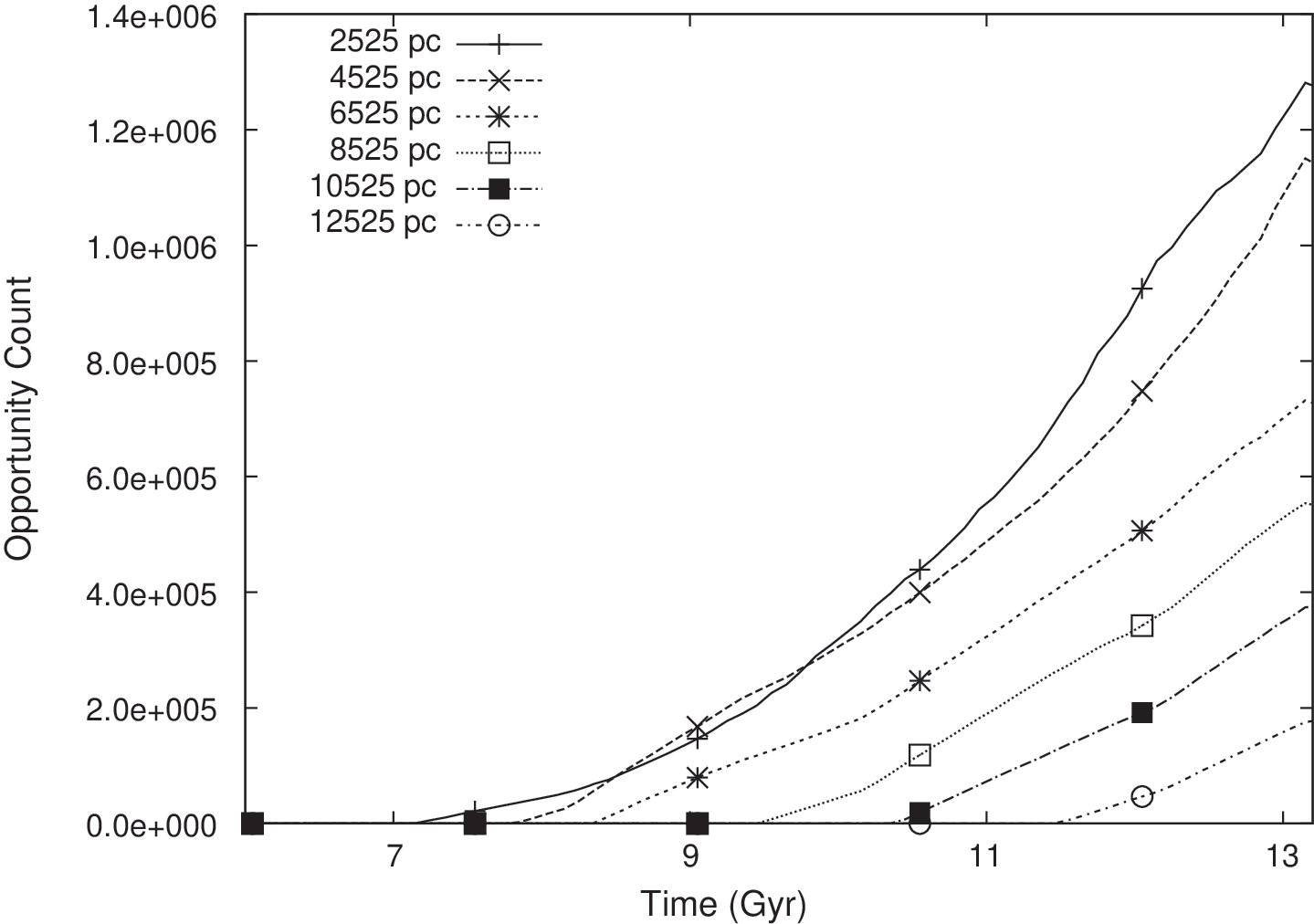
Opportunity counts versus epoch time (time since the formation of the Galaxy) for six cases of r and for T _thresh=0.6 Gyr. At any point on the time axis, the count on the vertical axis represents the total number of habitable planets on which there is currently an “active” opportunity.

At all radii, the number of opportunities is seen to increase monotonically with time. For smaller radii, the counts are higher due to the higher number density of habitable planets. Each curve stays at zero for a certain duration before beginning to rise. The time at which the rise begins is earlier at smaller radii, which is due to the higher average age of planets toward the inner Galaxy. At higher radii, the first opportunities for the emergence of intelligence do not occur until later times, once the planet ages reach the necessary threshold.

For all values of radius, the number of active opportunities thus far in galactic history is at its maximum at the present time. That is, the likelihood of intelligence emerging is right now the highest it has ever been. Furthermore, the trend of increasing propensity will continue into the future, likely for the next few billion years, as the metallicity increases throughout the disk, thus supporting higher planet formation rates. Additionally, contributing to the increasing propensity is the star formation rate, which has not been in significant decline in the past few billion years, and the fact that more time is available for the development of intelligent life on planets that currently exist in the Galaxy.

As previously mentioned, we focus on modeling planets in the galactic disk and have not considered the galactic bulge due to the complicated formation history and dynamical effects that may be important to consider in this region. Jiménez-Torres et al. (2013) modeled the dynamical effects of stellar flybys on planetary systems in discrete regions and found that different galactic environments may reduce the habitability of planets due to either (a) strong gravitational interactions that may perturb planetary systems or (b) weaker interactions that may perturb primordial material left over from planet formation, such as Oort cloud–like objects, which may cause a flux of material to impact the inner planets and potentially a mass extinction event. Since we have ignored the galactic bulge, we have not attempted to model these effects in this work. Stellar flybys may reduce the habitability of planets in different galactic environments and thus the propensity for intelligent life within the Milky Way.

We note that, while we have only considered the effects of SN sterilizations, there are other events that could decrease habitability in the near future, such as gamma ray bursts (GRBs). Piran and Jimenez (2014) examined the impact of GRBs on galactic habitability and concluded that, as GRBs are more likely to occur in the inner Galaxy and sterilize kiloparsec-scale regions, the outer Galaxy is a better place to find life. We note that there are some assumptions made in their work that will bear further analysis, specifically that long GRBs are found preferentially in low-metallicity dwarf galaxies, and that the assumption that the low-metallicity members of the disk population of the Milky Way can be equated with the low-metallicity dwarf hosts of GRBs in external galaxies may well not be true. Moreover, their analysis ignores the significant directional beaming of GRBs, which may allow the habitability of large regions of a galaxy in the vicinity of a GRB to be unaffected. The rate at which GRBs occur is also important to include, since sterilization by a GRB is not necessarily fatal to life in that region for the rest of galactic history (as our simulations model for SN extinctions). Finally, we note that the assumption that GRB rate scales with the stellar density is not dissimilar to the SNe rate scaling with stellar density. Our simulations of the impact of SNe show that, despite the higher SNe rate, the best place to search for intelligence is the inner Galaxy. The results of Piran and Jimenez (2014) suggest that a detailed simulation of the impact of GRBs could be a worthwhile future extension to the habitability models on which the present work is based. However, in the absence of detailed modeling, we can be confident in making the qualitative assertion that GRBs are unlikely to decrease habitability in the Milky Way to levels significantly lower than those currently experienced for two reasons: (i) the frequency of such events and their destructive power are not sufficient to significantly inhibit the propensity for intelligence over a large spatial extent and (ii) the general increase over time in the propensity for intelligence (due to increasing planet age) would tend to offset the negative impact of GRBs.

A further observation from Fig. 10 is that, at the time intelligence arose on Earth (approximately the present time), our model suggests a similar number density of active opportunities was present in the inner Galaxy more than 2 Gyr ago. This does not imply that other civilizations have actually emerged in the inner Galaxy, but it does offer some insight into the potential age of any such civilizations, should they exist.