Habitability of Waterworlds: Runaway Greenhouses,Atmospheric Expansion,and Multiple Climate States of Pure Water Atmospheres

Abstract

There are four different stable climate states for pure water atmospheres, as might exist on so-called “waterworlds.” I map these as a function of solar constant for planets ranging in size from Mars-sized to 10 Earth-mass. The states are as follows: globally ice covered (T _s⪅245 K), cold and damp (270⪅T _s⪅290 K), hot and moist (350⪅T _s⪅550 K), and very hot and dry (T _sx2A86;900 K). No stable climate exists for 290⪅T _s ⪅350 K or 550⪅T _s⪅900 K. The union of hot moist and cold damp climates describes the liquid water habitable zone, the width and location of which depends on planet mass. At each solar constant, two or three different climate states are stable. This is a consequence of strong nonlinearities in both thermal emission and the net absorption of sunlight.

Across the range of planet sizes, I account for the atmospheres expanding to high altitudes as they warm. The emitting and absorbing surfaces (optical depth of unity) move to high altitude, making their area larger than the planet surface, so more thermal radiation is emitted and more sunlight absorbed (the former dominates). The atmospheres of small planets expand more due to weaker gravity; the effective runaway greenhouse threshold is about 35 W m⁻² higher for Mars, 10 W m⁻² higher for Earth or Venus, but only a few W m⁻² higher for a 10 Earth-mass planet. There is an underlying (expansion-neglected) trend of increasing runaway greenhouse threshold with planetary size (40 W m⁻² higher for a 10 Earth-mass planet than for Mars). Summing these opposing trends means that Venus-sized (or slightly smaller) planets are most susceptible to a runaway greenhouse.

The habitable zone for pure water atmospheres is very narrow, with an insolation range of 0.07 times the solar constant. A wider habitable zone requires background gas and greenhouse gas: N₂ and CO₂ on Earth, which are biologically controlled. Thus, habitability depends on inhabitance. Key Words: Habitable zone—Runaway greenhouse—Waterworld—Climate. Astrobiology 15, 362–370.

1. Introduction

In this paper, I calculate the effect of changes to the vertical extent of pure water atmospheres on the radiation balance of waterworlds. As water atmospheres become hot and therefore thick, the area of the emitting and absorbing surface increases, modifying the planetary energy balance. This effect has been neglected in previous numerical calculations of the runaway greenhouse (Pollack, 1971; Watson et al., 1984; Abe and Matsui, 1988; Kasting, 1988; Goldblatt et al., 2013). With new calculations of the energy budget, I map out the various steady-state climates of water worlds as a function of planetary mass (from Mars-sized to 10 Earth masses) and incoming sunlight and hence describe the habitable zone.

For simplicity, I consider pure water atmospheres only. For an atmosphere with ∼1 bar of noncondensible gas, this gives a good approximation of the atmospheric structure when the atmosphere is hot, as the saturation vapor pressure of water would greatly exceed the dry air pressure. It is clearly a bad assumption for an atmosphere with ≳10 bar of noncondensible gas, like that of present Venus—but then Venus has lost its water already.

For waterworlds, a pure water atmosphere is the baseline assumption at all temperatures. Waterworlds are a hypothetical class of planet with some orders of magnitude more water than Earth, such that there is a deep liquid ocean separated from the rocky core by a thick layer of water ice (Léger et al., 2004). These seem straightforward to form dynamically (Raymond et al., 2004), and the mass-radius distribution of exoplanets between 1.5 and 4 Earth radii implies a high frequency of volatile-rich planets (Weiss and Marcy, 2014). The isolation of the ocean-atmosphere from the rocky core gives rise to the assumption of pure atmospheres. To have a pure atmosphere given the existence of surface inventories of C or N, one would suppose that they were dissolved in the ocean. Carbon dissolves easily, as seen on Earth. Nitrogen would have to be dissolved in the form of ammonia or nitrate, which would be plausible in the absence of life. In our solar system, Europa and Ganymede are akin to waterworlds and lack substantive atmospheres.

In understanding planetary energy balance, those of us whose atmospheric intuition is based on Earth will naturally think that the amount of radiation that escapes to space should depend upon the surface temperature. While much of the thermal spectrum is optically thick due to absorption by water, the region around 10 μm is not, so a fraction of surface radiation does escape directly to space. If the planet warms such that the ocean evaporates and the physical thickness of the atmosphere increases, the atmosphere will likewise become optically thick across the thermal spectrum such that no radiation from the surface will escape to space. Thermal emission would come dominantly from the atmospheric level where thermal optical depth is unity, which can be arbitrarily high above the surface but tends toward a constant temperature. For this reason, the thermal flux asymptotes to a constant with increasing surface temperature (see Nakajima et al., 1992, and Goldblatt and Watson, 2012, for reviews). Up-to-date calculations put this limit, which I refer to as the Simpson–Nakajima limit, around 280 W m² (Goldblatt et al., 2013). Likewise, the absorption of solar radiation asymptotes to a limit, too (Kasting, 1988), as both the levels of absorption and scattering optical depth of unity move high above the surface (Goldblatt et al., 2013).

Noting that emission of thermal radiation and absorption of sunlight happen in layers that are thin relative to the atmosphere facilitates straightforward scaling of plane-parallel radiative transfer calculations to an atmosphere that has become thick. I describe the methods for doing this briefly and discuss the changes in thermal flux emitted and solar flux absorbed in more detail. I then describe the four separate climate states of waterworlds, including a hot and moist (350 ⪅ T _s ⪅550 K) stable state, a finding that I believe to be novel.

Note that I use the phrase “atmospheric expansion” as a shorthand to refer to increases in the vertical extent of the atmosphere relative to Earth's atmosphere as surface temperature increases, hence expansion of area of the emitting and absorbing levels (surfaces) within the atmosphere. It does not imply vertical velocity or acceleration; the atmospheres that I consider are all in hydrostatic balance.

2. Methods

2.1. Model atmosphere and radiative transfer

My model atmosphere and radiative transfer methods follow those of Goldblatt et al. (2013) directly. Hence, I give a brief description only here; refer to the Methods and Supplementary Information of Goldblatt et al. (2013) for more detail.

As I consider pure water atmospheres only, the moist adiabat that typically describes the structure of planetary atmospheres simplifies to the saturation vapor pressure curve of water.

The mass range of the planets considered is from Mars (0.12 Earth mass) to 10 Earth mass, via a 0.3 Earth-mass planet, Venus (0.82 Earth mass), Earth, and a 3 Earth-mass planet. For the imaginary planets, the mass-radius is approximated by M/M _Earth=(r/r _Earth)^2.7 (Valencia et al., 2006).

Surface temperatures range between 220 and 2000 K. I define the structure as the saturation vapor pressure curve when the surface temperature is less than the critical point, or a dry adiabat merging to the saturation vapor pressure curve when surface temperature is supercritical. I take the total water inventory to be that which gives a surface pressure of 260 bar when the entire ocean evaporates, as on Earth. This is a quite arbitrary assumption, as the initial water inventory of a planet likely depends more on where it formed than its mass (compare Earth to Europa), and water inventory at some point in history depends on atmospheric evolution (compare Earth to Venus). However, given that the limiting fluxes are approached with less than a bar of atmospheric water (Goldblatt et al., 2013), this assumption is likely unimportant.

I omit clouds but use an artificially high surface albedo (0.25) in lieu of cloud albedo. This assumption is frequently used in habitable zone, early Earth climate, and runaway greenhouse studies (e.g., Kasting et al., 1984; Goldblatt et al., 2009a). This is not to say it is a good assumption (Goldblatt and Zahnle, 2011), only that the alternatives might be worse in this case. I have no intuition for cloud behavior or feedbacks in these atmospheres, so sidestepping this allows me to focus attention on the clear-sky behavior, which is complex and fascinating enough itself.

Radiative transfer calculations are done with the SMART code, written by David Crisp (Meadows and Crisp, 1996), modified to include Rayleigh scattering by water (Goldblatt et al., 2013). Spectral data are taken from HITEMP2012 (Rothman et al., 2010) (HITRAN does not have sufficient lines for thick atmospheres). The sign conventions are positive downward (heats the planet) for solar flux \documentclass{aastex}\usepackage{amsbsy}\usepackage{amsfonts}\usepackage{amssymb}\usepackage{bm}\usepackage{mathrsfs}\usepackage{pifont}\usepackage{stmaryrd}\usepackage{textcomp}\usepackage{portland, xspace}\usepackage{amsmath, amsxtra}\pagestyle{empty}\DeclareMathSizes{10}{9}{7}{6}\begin{document} \begin{align*}F_{ \rm solar} = F_{ \rm solar}^{ \downarrow} - F_{ \rm solar}^{ \uparrow} \tag{1}\end{align*} \end{document}

and positive upward (cools the planet) for thermal fluxes \documentclass{aastex}\usepackage{amsbsy}\usepackage{amsfonts}\usepackage{amssymb}\usepackage{bm}\usepackage{mathrsfs}\usepackage{pifont}\usepackage{stmaryrd}\usepackage{textcomp}\usepackage{portland, xspace}\usepackage{amsmath, amsxtra}\pagestyle{empty}\DeclareMathSizes{10}{9}{7}{6}\begin{document} \begin{align*}F_{ \rm thermal} = F_{ \rm thermal}^{ \uparrow} - F_{ \rm thermal}^{ \downarrow} \tag{2}\end{align*} \end{document}

and the net flux is positive downward \documentclass{aastex}\usepackage{amsbsy}\usepackage{amsfonts}\usepackage{amssymb}\usepackage{bm}\usepackage{mathrsfs}\usepackage{pifont}\usepackage{stmaryrd}\usepackage{textcomp}\usepackage{portland, xspace}\usepackage{amsmath, amsxtra}\pagestyle{empty}\DeclareMathSizes{10}{9}{7}{6}\begin{document} \begin{align*}F = F_{ \rm thermal} - F_{ \rm solar} \tag{3}\end{align*} \end{document}

2.2. Scaling fluxes for expanded atmospheres

A key property of runaway greenhouse atmospheres is that, for any given wavelength ν, emission of thermal radiation and absorption of solar radiation both dominantly occur in layers that are thin relative to the whole atmosphere. I approximate this as occurring at a single level at which the optical depth is unity (altitude z_τ ₌₁). As z_τ ₌₁ becomes nontrivial compared to the planetary radius, r ₀, the area of the emitting and absorbing surface of the planet increases. I thus define a scaling factor, \documentclass{aastex}\usepackage{amsbsy}\usepackage{amsfonts}\usepackage{amssymb}\usepackage{bm}\usepackage{mathrsfs}\usepackage{pifont}\usepackage{stmaryrd}\usepackage{textcomp}\usepackage{portland, xspace}\usepackage{amsmath, amsxtra}\pagestyle{empty}\DeclareMathSizes{10}{9}{7}{6}\begin{document} \begin{align*}a_ { \nu } = \frac { r_ { \tau = 1 } ( \nu ) } { r_0 } = \frac { r_0 + z_ { \tau = 1 } ( \nu ) } { r_0 } \tag { 4} \end{align*} \end{document}

to give the radiative flux absorbed or emitted per unit area of planetary surface from an expanded atmosphere. Changes to the size of the emitting and absorbing areas are not included in my SMART runs, so the flux from the expanded atmosphere is the product of the flux calculated in SMART and the scaling factor.

To find z_τ ₌₁, I begin with p_τ ₌₁, which SMART outputs as a function of wavelength. I solve for radius by integrating the hydrostatic equation up from the surface, allowing for variation in gravitational acceleration g with radius [g=g ₀(r ₀/r)², where g ₀ is gravity at the planetary surface]. \documentclass{aastex}\usepackage{amsbsy}\usepackage{amsfonts}\usepackage{amssymb}\usepackage{bm}\usepackage{mathrsfs}\usepackage{pifont}\usepackage{stmaryrd}\usepackage{textcomp}\usepackage{portland, xspace}\usepackage{amsmath, amsxtra}\pagestyle{empty}\DeclareMathSizes{10}{9}{7}{6}\begin{document} \begin{align*} \frac { dp } { dr } = - \rho g = - \rho g_0 \left( \frac { r } { r_0 } \right) ^2 \tag { 5 } \end{align*} \end{document}

Given that the ideal gas law breaks down at the high temperatures considered here, I take density ρ=ρ(p, T) from the IAPWS95 formulation (Wager and Pruss, 2002; Junglas, 2008) and solve numerically to give z=z(p). Vectors of altitude at which τ=1 and scaling factor a, both as a function of wavelength, are found directly.

It is convenient to reduce a two to broadband scaling factors, for the solar radiation and thermal radiation. To do so, I take a weighted sum of the product of the vector scaling factor and the relevant irradiance. For thermal radiation, the spectrum of top-of-atmosphere outgoing thermal flux, \documentclass{aastex}\usepackage{amsbsy}\usepackage{amsfonts}\usepackage{amssymb}\usepackage{bm}\usepackage{mathrsfs}\usepackage{pifont}\usepackage{stmaryrd}\usepackage{textcomp}\usepackage{portland, xspace}\usepackage{amsmath, amsxtra}\pagestyle{empty}\DeclareMathSizes{10}{9}{7}{6}\begin{document}$${ \bf I}_{ \rm thermal , TOA}^{ \uparrow}$$ \end{document} , is appropriate, giving \documentclass{aastex}\usepackage{amsbsy}\usepackage{amsfonts}\usepackage{amssymb}\usepackage{bm}\usepackage{mathrsfs}\usepackage{pifont}\usepackage{stmaryrd}\usepackage{textcomp}\usepackage{portland, xspace}\usepackage{amsmath, amsxtra}\pagestyle{empty}\DeclareMathSizes{10}{9}{7}{6}\begin{document} \begin{align*} { a } _ { \rm thermal } = \frac { \sum \left( { \bf a } \cdot { \bf I } _ { \rm thermal , TOA } ^ { \uparrow } \right) } { \sum { \bf I } _ { \rm thermal , TOA } ^ { \uparrow }} \tag { 6 } \end{align*} \end{document}

For solar radiation, the spectrum of incoming sunlight at the top of the atmosphere, \documentclass{aastex}\usepackage{amsbsy}\usepackage{amsfonts}\usepackage{amssymb}\usepackage{bm}\usepackage{mathrsfs}\usepackage{pifont}\usepackage{stmaryrd}\usepackage{textcomp}\usepackage{portland, xspace}\usepackage{amsmath, amsxtra}\pagestyle{empty}\DeclareMathSizes{10}{9}{7}{6}\begin{document}$${ \bf I}_{ \rm solar , TOA}^{ \downarrow}$$ \end{document} , is appropriate, giving \documentclass{aastex}\usepackage{amsbsy}\usepackage{amsfonts}\usepackage{amssymb}\usepackage{bm}\usepackage{mathrsfs}\usepackage{pifont}\usepackage{stmaryrd}\usepackage{textcomp}\usepackage{portland, xspace}\usepackage{amsmath, amsxtra}\pagestyle{empty}\DeclareMathSizes{10}{9}{7}{6}\begin{document} \begin{align*} { a } _ { \rm solar } = \frac { \sum \left( { \bf a } \cdot { \bf I } _ { \rm solar , TOA } ^ { \downarrow } \right)} { \sum { \bf I } _ { \rm solar , TOA } ^ { \downarrow } } \tag{ 7 } \end{align*} \end{document}

Fluxes from the expanded atmospheres, F _expand, are directly related to fluxes calculated by SMART, F _orig: \documentclass{aastex}\usepackage{amsbsy}\usepackage{amsfonts}\usepackage{amssymb}\usepackage{bm}\usepackage{mathrsfs}\usepackage{pifont}\usepackage{stmaryrd}\usepackage{textcomp}\usepackage{portland, xspace}\usepackage{amsmath, amsxtra}\pagestyle{empty}\DeclareMathSizes{10}{9}{7}{6}\begin{document} \begin{align*}F_{ \rm expand , thermal} = {a}_{ \rm thermal} F_{ \rm orig , thermal} \tag{8}\end{align*} \end{document} \documentclass{aastex}\usepackage{amsbsy}\usepackage{amsfonts}\usepackage{amssymb}\usepackage{bm}\usepackage{mathrsfs}\usepackage{pifont}\usepackage{stmaryrd}\usepackage{textcomp}\usepackage{portland, xspace}\usepackage{amsmath, amsxtra}\pagestyle{empty}\DeclareMathSizes{10}{9}{7}{6}\begin{document} \begin{align*}F_{ \rm expand , solar} = {a}_{ \rm solar} F_{ \rm orig , solar} \tag{9}\end{align*} \end{document}

By derivation, F _expand are fluxes per unit area of planetary surface. These are useful because they enable one to consider changes in the energy budget with a fixed reference frame and so understand changes with increases in atmospheric size. However, they are somewhat nonphysical in that a locally placed radiometer would measure the unexpanded flux.

Strictly, the plane parallel assumption employed in most radiation codes (SMART included) requires that the vertical extent of the atmosphere be smaller than the planetary radius. For the warmest atmospheres on Mars, this becomes somewhat questionable, as optical depth of unity is around 1000 km, whereas the radius at the surface is 3390 km. However, given that the limiting fluxes are determined in thin layers, the effect of sphericity should be minimal, and the scaling approach we use here should give an answer which is correct to first order. The alternative, of full 3-D radiative transfer calculations, is prohibitively difficult and expensive.

2.3. Steady states for climate

Overall temperature change of a planet is related to top-of-atmosphere fluxes—sunlight absorbed by the planet and top-of-atmosphere thermal emission. For brevity: \documentclass{aastex}\usepackage{amsbsy}\usepackage{amsfonts}\usepackage{amssymb}\usepackage{bm}\usepackage{mathrsfs}\usepackage{pifont}\usepackage{stmaryrd}\usepackage{textcomp}\usepackage{portland, xspace}\usepackage{amsmath, amsxtra}\pagestyle{empty}\DeclareMathSizes{10}{9}{7}{6}\begin{document} \begin{align*}{ \cal F}_{ \rm solar} = F_{ \rm solar , TOA} = F_{ \rm solar , TOA}^{ \downarrow} - F_{ \rm solar , TOA}^{ \uparrow} \tag{10}\end{align*} \end{document} \documentclass{aastex}\usepackage{amsbsy}\usepackage{amsfonts}\usepackage{amssymb}\usepackage{bm}\usepackage{mathrsfs}\usepackage{pifont}\usepackage{stmaryrd}\usepackage{textcomp}\usepackage{portland, xspace}\usepackage{amsmath, amsxtra}\pagestyle{empty}\DeclareMathSizes{10}{9}{7}{6}\begin{document} \begin{align*}{ \cal F}_{ \rm thermal} = F_{ \rm thermal , TOA} = F_{ \rm thermal , TOA}^{ \uparrow} \tag{11}\end{align*} \end{document}

Scaling \documentclass{aastex}\usepackage{amsbsy}\usepackage{amsfonts}\usepackage{amssymb}\usepackage{bm}\usepackage{mathrsfs}\usepackage{pifont}\usepackage{stmaryrd}\usepackage{textcomp}\usepackage{portland, xspace}\usepackage{amsmath, amsxtra}\pagestyle{empty}\DeclareMathSizes{10}{9}{7}{6}\begin{document}$${ \cal F}_{ \rm solar}$$ \end{document} by a constant S/S ₀ can be used to reflect changing solar constant (due to orbital distance or stellar evolution), taking the reference value to be at Earth's orbit now, S ₀=1368 W m⁻². Thus \documentclass{aastex}\usepackage{amsbsy}\usepackage{amsfonts}\usepackage{amssymb}\usepackage{bm}\usepackage{mathrsfs}\usepackage{pifont}\usepackage{stmaryrd}\usepackage{textcomp}\usepackage{portland, xspace}\usepackage{amsmath, amsxtra}\pagestyle{empty}\DeclareMathSizes{10}{9}{7}{6}\begin{document} \begin{align*} { \cal F } = { \cal F } _ { \rm thermal } - \frac{ S } { S_0 } { \cal F } _ { \rm solar } \tag { 12 } \end{align*} \end{document}

\documentclass{aastex}\usepackage{amsbsy}\usepackage{amsfonts}\usepackage{amssymb}\usepackage{bm}\usepackage{mathrsfs}\usepackage{pifont}\usepackage{stmaryrd}\usepackage{textcomp}\usepackage{portland, xspace}\usepackage{amsmath, amsxtra}\pagestyle{empty}\DeclareMathSizes{10}{9}{7}{6}\begin{document}$${ \cal F} = 0$$ \end{document} implies steady state for climate. With \documentclass{aastex}\usepackage{amsbsy}\usepackage{amsfonts}\usepackage{amssymb}\usepackage{bm}\usepackage{mathrsfs}\usepackage{pifont}\usepackage{stmaryrd}\usepackage{textcomp}\usepackage{portland, xspace}\usepackage{amsmath, amsxtra}\pagestyle{empty}\DeclareMathSizes{10}{9}{7}{6}\begin{document}$${ \cal F}$$ \end{document} defined positive upward, \documentclass{aastex}\usepackage{amsbsy}\usepackage{amsfonts}\usepackage{amssymb}\usepackage{bm}\usepackage{mathrsfs}\usepackage{pifont}\usepackage{stmaryrd}\usepackage{textcomp}\usepackage{portland, xspace}\usepackage{amsmath, amsxtra}\pagestyle{empty}\DeclareMathSizes{10}{9}{7}{6}\begin{document}$$ \frac { d { \cal F } } { dT_ { \rm s } } > 0$$ \end{document} gives a stable steady state, and \documentclass{aastex}\usepackage{amsbsy}\usepackage{amsfonts}\usepackage{amssymb}\usepackage{bm}\usepackage{mathrsfs}\usepackage{pifont}\usepackage{stmaryrd}\usepackage{textcomp}\usepackage{portland, xspace}\usepackage{amsmath, amsxtra}\pagestyle{empty}\DeclareMathSizes{10}{9}{7}{6}\begin{document}$$ \frac { d { \cal F } } { dT_ { \rm s } } < 0$$ \end{document} gives an unstable steady state.

In my radiative transfer calculations, I assumed a fixed surface albedo, α_s=0.25. To include ice–albedo feedback in the climate calculations, I set surface albedo to represent an icy surface (α_s=0.65) when temperatures are low and vary smoothly to the standard value via a hyperbolic tangent (e.g., Saltzman, 2002): \documentclass{aastex}\usepackage{amsbsy}\usepackage{amsfonts}\usepackage{amssymb}\usepackage{bm}\usepackage{mathrsfs}\usepackage{pifont}\usepackage{stmaryrd}\usepackage{textcomp}\usepackage{portland, xspace}\usepackage{amsmath, amsxtra}\pagestyle{empty}\DeclareMathSizes{10}{9}{7}{6}\begin{document} \begin{align*}\alpha_ { \rm s } = 0.45 - 0.2 \ { \rm tanh } \left[ \frac { \pi } { 25 } ( T_ { \rm s } - 255 ) \right] \tag { 13 } \end{align*} \end{document}

The purpose of this is to give a schematic representation of ice–albedo feedback, not to accurately predict the bifurcation points.

A changed α_s changes the upward thermal flux vector \documentclass{aastex}\usepackage{amsbsy}\usepackage{amsfonts}\usepackage{amssymb}\usepackage{bm}\usepackage{mathrsfs}\usepackage{pifont}\usepackage{stmaryrd}\usepackage{textcomp}\usepackage{portland, xspace}\usepackage{amsmath, amsxtra}\pagestyle{empty}\DeclareMathSizes{10}{9}{7}{6}\begin{document}$$F_{ \rm solar}^{ \uparrow}$$ \end{document} only. \documentclass{aastex}\usepackage{amsbsy}\usepackage{amsfonts}\usepackage{amssymb}\usepackage{bm}\usepackage{mathrsfs}\usepackage{pifont}\usepackage{stmaryrd}\usepackage{textcomp}\usepackage{portland, xspace}\usepackage{amsmath, amsxtra}\pagestyle{empty}\DeclareMathSizes{10}{9}{7}{6}\begin{document}$$F_{ \rm solar}^{ \uparrow}$$ \end{document} is attenuated by both scattering and absorption. The source is, in general, a function of both scattering (of downward flux) and the surface source. Fortunately, the cold and thin atmospheres for which albedo is adjusted have negligible scattering optical depth; so the source is purely surface radiation, and attenuation is only by absorption. Thus, scaling \documentclass{aastex}\usepackage{amsbsy}\usepackage{amsfonts}\usepackage{amssymb}\usepackage{bm}\usepackage{mathrsfs}\usepackage{pifont}\usepackage{stmaryrd}\usepackage{textcomp}\usepackage{portland, xspace}\usepackage{amsmath, amsxtra}\pagestyle{empty}\DeclareMathSizes{10}{9}{7}{6}\begin{document}$$F_{ \rm solar}^{ \uparrow}$$ \end{document} to the new albedo can be done directly.

3. Results

3.1. The runaway greenhouse in expanded atmospheres

The altitude at which absorption optical depth is unity is shown for Mars, Earth, and a 10 Earth-mass planet (Fig. 1). For more massive planets, the vertical extent of the atmosphere is small compared to radius, even when the atmosphere is thick. By contrast, for small planets like Mars the atmosphere extends to high altitudes, especially when the surface is warm. In the middle, for Earth, optical depth of unity is at several hundred kilometers altitude for hot atmospheres, so expansion will matter.

FIG. 1.

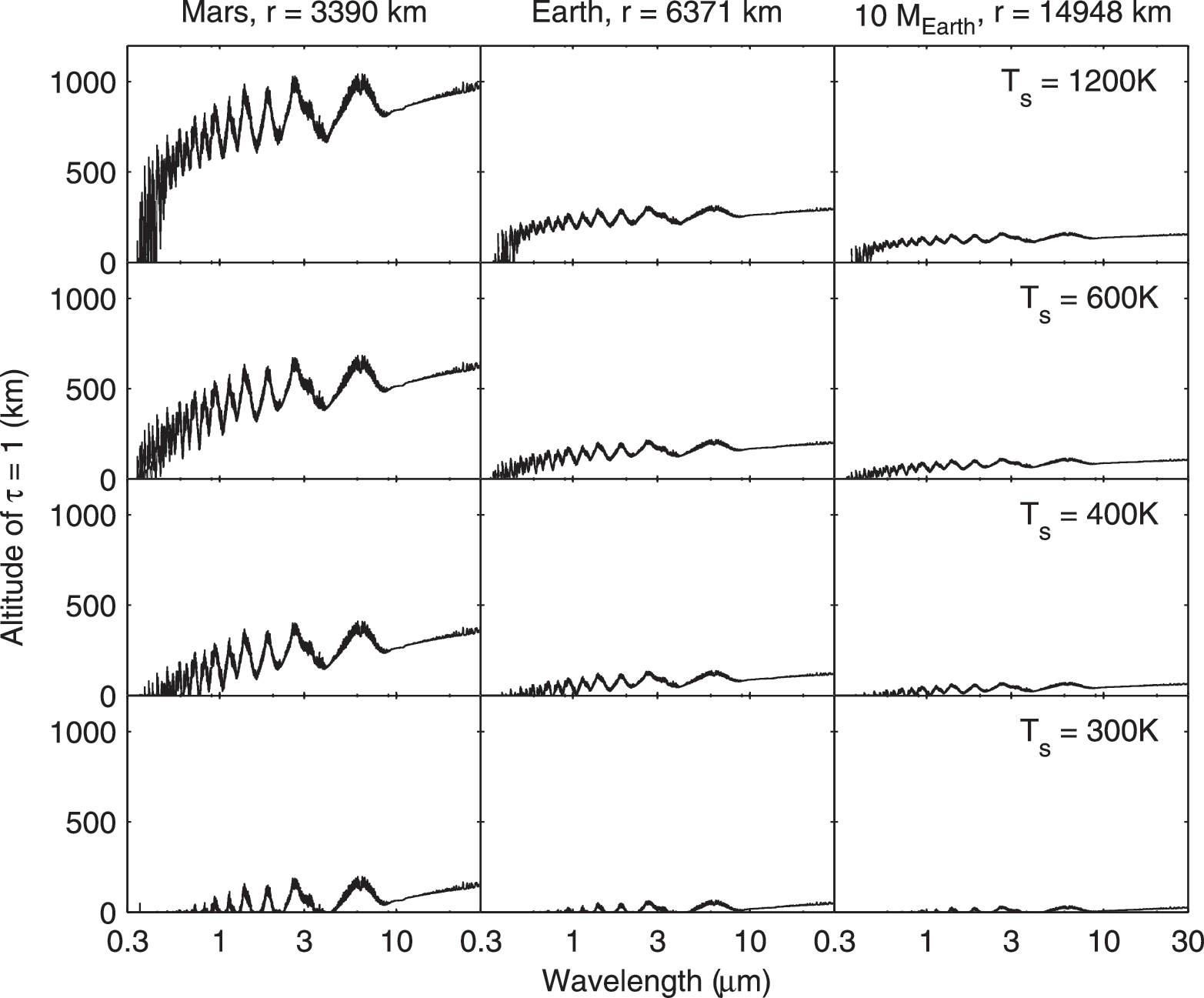
Altitude at which absorption optical depth is unity (z _τ ₌₁) with changing temperature for three example planets of radius r. This is the height at which effective thermal emission to space and absorption of solar radiation will dominantly occur. Note how, for heavier planets, z _τ ₌₁ << r, so atmospheric expansion has little effect, whereas for small planets z _τ ₌₁ ∼ r, so atmospheric expansion is of first-order importance.

Figure 2 shows the scaling factor, absorbed solar flux ( \documentclass{aastex}\usepackage{amsbsy}\usepackage{amsfonts}\usepackage{amssymb}\usepackage{bm}\usepackage{mathrsfs}\usepackage{pifont}\usepackage{stmaryrd}\usepackage{textcomp}\usepackage{portland, xspace}\usepackage{amsmath, amsxtra}\pagestyle{empty}\DeclareMathSizes{10}{9}{7}{6}\begin{document}$${ \cal F}_{ \rm solar}$$ \end{document} ), outgoing thermal flux ( \documentclass{aastex}\usepackage{amsbsy}\usepackage{amsfonts}\usepackage{amssymb}\usepackage{bm}\usepackage{mathrsfs}\usepackage{pifont}\usepackage{stmaryrd}\usepackage{textcomp}\usepackage{portland, xspace}\usepackage{amsmath, amsxtra}\pagestyle{empty}\DeclareMathSizes{10}{9}{7}{6}\begin{document}$${ \cal F}_{ \rm thermal}$$ \end{document} ), and net flux ( \documentclass{aastex}\usepackage{amsbsy}\usepackage{amsfonts}\usepackage{amssymb}\usepackage{bm}\usepackage{mathrsfs}\usepackage{pifont}\usepackage{stmaryrd}\usepackage{textcomp}\usepackage{portland, xspace}\usepackage{amsmath, amsxtra}\pagestyle{empty}\DeclareMathSizes{10}{9}{7}{6}\begin{document}$${ \cal F}$$ \end{document} ) for each planet as a function of temperature, both with expansion neglected and considered. I first describe the properties of expansion-neglected fluxes (gray lines) for solar, thermal, and net fluxes, as these illustrate important points of the atmospheric physics, then move on to consideration of expansion. \documentclass{aastex}\usepackage{amsbsy}\usepackage{amsfonts}\usepackage{amssymb}\usepackage{bm}\usepackage{mathrsfs}\usepackage{pifont}\usepackage{stmaryrd}\usepackage{textcomp}\usepackage{portland, xspace}\usepackage{amsmath, amsxtra}\pagestyle{empty}\DeclareMathSizes{10}{9}{7}{6}\begin{document}$${ \cal F}_{ \rm solar}$$ \end{document} initially increases with temperature but subsequently decreases before asymptoting to a constant. Recall that increasing temperature is accompanied by increasing atmospheric mass, as ocean evaporates. The initial increase in \documentclass{aastex}\usepackage{amsbsy}\usepackage{amsfonts}\usepackage{amssymb}\usepackage{bm}\usepackage{mathrsfs}\usepackage{pifont}\usepackage{stmaryrd}\usepackage{textcomp}\usepackage{portland, xspace}\usepackage{amsmath, amsxtra}\pagestyle{empty}\DeclareMathSizes{10}{9}{7}{6}\begin{document}$${ \cal F}_{ \rm solar}$$ \end{document} occurs as there is more molecular absorption as the atmosphere becomes thicker; referring back to Fig. 1, note how the atmosphere is optically thin for short wavelengths at low temperatures but becomes optically thick at all wavelengths as temperatures increase. With a thicker atmosphere still, the atmosphere becomes optically thick with respect to Rayleigh scattering, too; bluer light that may otherwise have been absorbed at the surface, low in the atmosphere or on the upward path, is reflected by the atmosphere. This causes the decrease in \documentclass{aastex}\usepackage{amsbsy}\usepackage{amsfonts}\usepackage{amssymb}\usepackage{bm}\usepackage{mathrsfs}\usepackage{pifont}\usepackage{stmaryrd}\usepackage{textcomp}\usepackage{portland, xspace}\usepackage{amsmath, amsxtra}\pagestyle{empty}\DeclareMathSizes{10}{9}{7}{6}\begin{document}$${ \cal F}_{ \rm solar}$$ \end{document} The asymptotic value for \documentclass{aastex}\usepackage{amsbsy}\usepackage{amsfonts}\usepackage{amssymb}\usepackage{bm}\usepackage{mathrsfs}\usepackage{pifont}\usepackage{stmaryrd}\usepackage{textcomp}\usepackage{portland, xspace}\usepackage{amsmath, amsxtra}\pagestyle{empty}\DeclareMathSizes{10}{9}{7}{6}\begin{document}$${ \cal F}_{ \rm solar}$$ \end{document} reflects the balance between absorption and scattering cross sections (Goldblatt et al., 2013).

FIG. 2.

For each planet considered (columns): (a) Scaling factor; the ratio of squares of radius at which atmospheric optical depth is unity r _τ ₌₁=z _τ ₌₁+r ₀ to the radius of the planet surface, r ₀. This is the ratio of how much energy will be absorbed or emitted by the atmosphere relative to an atmosphere with equivalent optical properties but negligible vertical extent. Solar is dashed, thermal dash-dotted. (b) Net absorbed solar flux (top-of-atmosphere incoming minus outgoing) given a solar constant equal to modern Earth's for atmospheres where expansion is neglected (gray) and considered (black). (c) Outgoing thermal flux at the top of the atmosphere for atmospheres where expansion is neglected (gray) and considered (black). (d) Net outgoing radiation (outgoing thermal minus absorbed solar) for atmospheres where expansion is neglected (gray) and considered (black). Negative values indicate planetary warming, whereas positive values are planetary cooling. Stable states have a zero net outgoing flux.

Thermal fluxes are more straightforward, as in the infrared the atmosphere is absorbing but non-scattering. Increasing surface temperature increases surface emission by Stefan–Boltzmann law. With low surface temperature, the atmosphere is physically thin and optically thin. Surface radiation reaches space, and \documentclass{aastex}\usepackage{amsbsy}\usepackage{amsfonts}\usepackage{amssymb}\usepackage{bm}\usepackage{mathrsfs}\usepackage{pifont}\usepackage{stmaryrd}\usepackage{textcomp}\usepackage{portland, xspace}\usepackage{amsmath, amsxtra}\pagestyle{empty}\DeclareMathSizes{10}{9}{7}{6}\begin{document}$${ \cal F}_{ \rm thermal}$$ \end{document} increases with surface temperature. As temperature and atmospheric mass increase, the level from which thermal emission occurs moves up in the atmosphere, assumes a constant temperature, and \documentclass{aastex}\usepackage{amsbsy}\usepackage{amsfonts}\usepackage{amssymb}\usepackage{bm}\usepackage{mathrsfs}\usepackage{pifont}\usepackage{stmaryrd}\usepackage{textcomp}\usepackage{portland, xspace}\usepackage{amsmath, amsxtra}\pagestyle{empty}\DeclareMathSizes{10}{9}{7}{6}\begin{document}$${ \cal F}_{ \rm thermal}$$ \end{document} asymptotes to a constant (Nakajima et al., 1992; Goldblatt and Watson, 2012; Goldblatt et al., 2013). When surface temperatures are >1500 K, \documentclass{aastex}\usepackage{amsbsy}\usepackage{amsfonts}\usepackage{amssymb}\usepackage{bm}\usepackage{mathrsfs}\usepackage{pifont}\usepackage{stmaryrd}\usepackage{textcomp}\usepackage{portland, xspace}\usepackage{amsmath, amsxtra}\pagestyle{empty}\DeclareMathSizes{10}{9}{7}{6}\begin{document}$${ \cal F}_{ \rm thermal}$$ \end{document} increases again as the high troposphere becomes sufficiently hot to emit in the 4 μm water vapor window (Goldblatt et al., 2013). Planetary energy balance is determined by \documentclass{aastex}\usepackage{amsbsy}\usepackage{amsfonts}\usepackage{amssymb}\usepackage{bm}\usepackage{mathrsfs}\usepackage{pifont}\usepackage{stmaryrd}\usepackage{textcomp}\usepackage{portland, xspace}\usepackage{amsmath, amsxtra}\pagestyle{empty}\DeclareMathSizes{10}{9}{7}{6}\begin{document}$${ \cal F} = { \cal F}_{ \rm thermal} - { \cal F}_{ \rm solar}$$ \end{document} (expansion is still neglected); combining cubic nonlinearities from both thermal and solar streams gives a quintic nonlinearity. The order of processes is as follows: (1) Increasing surface temperature initially increases \documentclass{aastex}\usepackage{amsbsy}\usepackage{amsfonts}\usepackage{amssymb}\usepackage{bm}\usepackage{mathrsfs}\usepackage{pifont}\usepackage{stmaryrd}\usepackage{textcomp}\usepackage{portland, xspace}\usepackage{amsmath, amsxtra}\pagestyle{empty}\DeclareMathSizes{10}{9}{7}{6}\begin{document}$${ \cal F}_{ \rm thermal}$$ \end{document} , causing \documentclass{aastex}\usepackage{amsbsy}\usepackage{amsfonts}\usepackage{amssymb}\usepackage{bm}\usepackage{mathrsfs}\usepackage{pifont}\usepackage{stmaryrd}\usepackage{textcomp}\usepackage{portland, xspace}\usepackage{amsmath, amsxtra}\pagestyle{empty}\DeclareMathSizes{10}{9}{7}{6}\begin{document}$${ \cal F}$$ \end{document} to increase to a local maximum. (2) Increase in \documentclass{aastex}\usepackage{amsbsy}\usepackage{amsfonts}\usepackage{amssymb}\usepackage{bm}\usepackage{mathrsfs}\usepackage{pifont}\usepackage{stmaryrd}\usepackage{textcomp}\usepackage{portland, xspace}\usepackage{amsmath, amsxtra}\pagestyle{empty}\DeclareMathSizes{10}{9}{7}{6}\begin{document}$${ \cal F}_{ \rm solar}$$ \end{document} due to absorption causes \documentclass{aastex}\usepackage{amsbsy}\usepackage{amsfonts}\usepackage{amssymb}\usepackage{bm}\usepackage{mathrsfs}\usepackage{pifont}\usepackage{stmaryrd}\usepackage{textcomp}\usepackage{portland, xspace}\usepackage{amsmath, amsxtra}\pagestyle{empty}\DeclareMathSizes{10}{9}{7}{6}\begin{document}$${ \cal F}$$ \end{document} to decrease to a local minimum. (3) Increased Rayleigh scattering decreases \documentclass{aastex}\usepackage{amsbsy}\usepackage{amsfonts}\usepackage{amssymb}\usepackage{bm}\usepackage{mathrsfs}\usepackage{pifont}\usepackage{stmaryrd}\usepackage{textcomp}\usepackage{portland, xspace}\usepackage{amsmath, amsxtra}\pagestyle{empty}\DeclareMathSizes{10}{9}{7}{6}\begin{document}$${ \cal F}_{ \rm solar}$$ \end{document} , allowing \documentclass{aastex}\usepackage{amsbsy}\usepackage{amsfonts}\usepackage{amssymb}\usepackage{bm}\usepackage{mathrsfs}\usepackage{pifont}\usepackage{stmaryrd}\usepackage{textcomp}\usepackage{portland, xspace}\usepackage{amsmath, amsxtra}\pagestyle{empty}\DeclareMathSizes{10}{9}{7}{6}\begin{document}$${ \cal F}$$ \end{document} to increase. (4) Both \documentclass{aastex}\usepackage{amsbsy}\usepackage{amsfonts}\usepackage{amssymb}\usepackage{bm}\usepackage{mathrsfs}\usepackage{pifont}\usepackage{stmaryrd}\usepackage{textcomp}\usepackage{portland, xspace}\usepackage{amsmath, amsxtra}\pagestyle{empty}\DeclareMathSizes{10}{9}{7}{6}\begin{document}$${ \cal F}_{ \rm solar}$$ \end{document} and \documentclass{aastex}\usepackage{amsbsy}\usepackage{amsfonts}\usepackage{amssymb}\usepackage{bm}\usepackage{mathrsfs}\usepackage{pifont}\usepackage{stmaryrd}\usepackage{textcomp}\usepackage{portland, xspace}\usepackage{amsmath, amsxtra}\pagestyle{empty}\DeclareMathSizes{10}{9}{7}{6}\begin{document}$${ \cal F}_{ \rm thermal}$$ \end{document} have reached asymptotic values, so \documentclass{aastex}\usepackage{amsbsy}\usepackage{amsfonts}\usepackage{amssymb}\usepackage{bm}\usepackage{mathrsfs}\usepackage{pifont}\usepackage{stmaryrd}\usepackage{textcomp}\usepackage{portland, xspace}\usepackage{amsmath, amsxtra}\pagestyle{empty}\DeclareMathSizes{10}{9}{7}{6}\begin{document}$${ \cal F}$$ \end{document} is constant. (5) Finally, 4 μm thermal emission increases \documentclass{aastex}\usepackage{amsbsy}\usepackage{amsfonts}\usepackage{amssymb}\usepackage{bm}\usepackage{mathrsfs}\usepackage{pifont}\usepackage{stmaryrd}\usepackage{textcomp}\usepackage{portland, xspace}\usepackage{amsmath, amsxtra}\pagestyle{empty}\DeclareMathSizes{10}{9}{7}{6}\begin{document}$${ \cal F}_{ \rm thermal}$$ \end{document} and \documentclass{aastex}\usepackage{amsbsy}\usepackage{amsfonts}\usepackage{amssymb}\usepackage{bm}\usepackage{mathrsfs}\usepackage{pifont}\usepackage{stmaryrd}\usepackage{textcomp}\usepackage{portland, xspace}\usepackage{amsmath, amsxtra}\pagestyle{empty}\DeclareMathSizes{10}{9}{7}{6}\begin{document}$${ \cal F}$$ \end{document} .

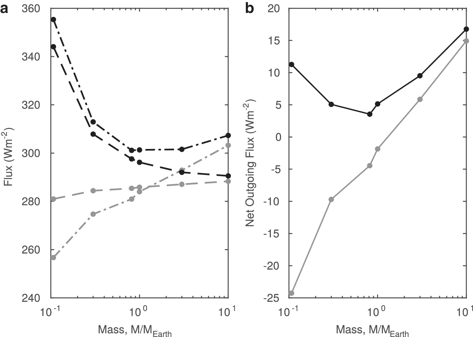
The asymptotic flux limits vary with planetary mass (Fig. 3). Both \documentclass{aastex}\usepackage{amsbsy}\usepackage{amsfonts}\usepackage{amssymb}\usepackage{bm}\usepackage{mathrsfs}\usepackage{pifont}\usepackage{stmaryrd}\usepackage{textcomp}\usepackage{portland, xspace}\usepackage{amsmath, amsxtra}\pagestyle{empty}\DeclareMathSizes{10}{9}{7}{6}\begin{document}$${ \cal F}_{ \rm solar}$$ \end{document} and \documentclass{aastex}\usepackage{amsbsy}\usepackage{amsfonts}\usepackage{amssymb}\usepackage{bm}\usepackage{mathrsfs}\usepackage{pifont}\usepackage{stmaryrd}\usepackage{textcomp}\usepackage{portland, xspace}\usepackage{amsmath, amsxtra}\pagestyle{empty}\DeclareMathSizes{10}{9}{7}{6}\begin{document}$${ \cal F}_{ \rm thermal}$$ \end{document} are bigger on heavier planets, though somewhat different processes are in effect. Solar radiation absorbed depends on a balance between Rayleigh scattering and absorption cross sections. Rayleigh scattering cross section is independent of pressure, so scattering optical depth is proportional simply to the number of molecules in the optical path. By contrast, absorption cross section does depend on ambient pressure, as absorption lines are broadened by pressure. With a more massive planet (higher g), the same number of molecules has a greater weight and so exerts more pressure, thereby increasing the absorption cross section. Hence, the ratio of absorption to scattering cross sections is larger, and more radiation is absorbed.

FIG. 3.

(a) Radiation limits, taken as the flux at 645 K, as a function of planetary mass. Net absorbed solar radiation as a dashed line given a solar constant equal to modern Earth's, outgoing thermal radiation as a dash-dotted line, for atmospheres where expansion is neglected (gray) and considered (black). (b) Net outgoing radiation (outgoing thermal minus absorbed solar) as a function of planet mass for atmospheres where expansion is neglected (gray) and considered (black).

Outgoing thermal flux depends on the temperature at the level of optical depth of unity. With atmospheric structure following the saturation vapor pressure curve, temperature is uniquely a function of pressure. With higher g, a smaller mass is required above some level to give the same pressure. Conversely, if to first approximation a fixed mass is required to give optical depth of unity, then under higher g the base of this layer will experience higher pressure and hence be at higher temperature, so more radiation will be omitted. Due to pressure-broadening of absorption lines, less mass is actually required at higher g, weakening this dependence (Pierrehumbert, 2010; Goldblatt et al., 2013). This behavior can be seen in Fig. 3.

Now that the properties of the fluxes with expansion neglected have been discussed, the effect of expansion of the atmosphere can be considered. I have restricted my analysis to atmospheres in which hydrostatic balance applies (that is, not considered Europa or Ganymede, where massive hydrodynamic escape is confounding). The isothermal case is instructive; pressure decreases exponentially with altitude \documentclass{aastex}\usepackage{amsbsy}\usepackage{amsfonts}\usepackage{amssymb}\usepackage{bm}\usepackage{mathrsfs}\usepackage{pifont}\usepackage{stmaryrd}\usepackage{textcomp}\usepackage{portland, xspace}\usepackage{amsmath, amsxtra}\pagestyle{empty}\DeclareMathSizes{10}{9}{7}{6}\begin{document} \begin{align*}p = p_0 \exp \left( \frac { - z } { H } \right) \tag { 14 } \end{align*} \end{document}

where the scale height \documentclass{aastex}\usepackage{amsbsy}\usepackage{amsfonts}\usepackage{amssymb}\usepackage{bm}\usepackage{mathrsfs}\usepackage{pifont}\usepackage{stmaryrd}\usepackage{textcomp}\usepackage{portland, xspace}\usepackage{amsmath, amsxtra}\pagestyle{empty}\DeclareMathSizes{10}{9}{7}{6}\begin{document}$$H = \frac { RT } { Mg } $$ \end{document} (R is universal gas constant, M molar mass). Hence, the altitude of some pressure level \documentclass{aastex}\usepackage{amsbsy}\usepackage{amsfonts}\usepackage{amssymb}\usepackage{bm}\usepackage{mathrsfs}\usepackage{pifont}\usepackage{stmaryrd}\usepackage{textcomp}\usepackage{portland, xspace}\usepackage{amsmath, amsxtra}\pagestyle{empty}\DeclareMathSizes{10}{9}{7}{6}\begin{document} \begin{align*}z = - \frac { 1 } { g } \cdot \frac { RT } { M } \ln \left( \frac { p } { p_0 } \right) \tag { 15 } \end{align*} \end{document}

is inversely proportional to gravity. Expansion thus affects small planets greatly but big planets far less; the difference between expanded and unexpanded fluxes becomes increasingly large as planets become smaller than Venus (Fig. 3). With water absorbing thermal radiation more strongly than solar radiation, the scaling factor for thermal radiation is always larger. The emitting surface becomes bigger, but this is largely offset by a bigger absorbing area (Fig. 2). For planets of 0.3 M _Earth and larger, these cancel such that \documentclass{aastex}\usepackage{amsbsy}\usepackage{amsfonts}\usepackage{amssymb}\usepackage{bm}\usepackage{mathrsfs}\usepackage{pifont}\usepackage{stmaryrd}\usepackage{textcomp}\usepackage{portland, xspace}\usepackage{amsmath, amsxtra}\pagestyle{empty}\DeclareMathSizes{10}{9}{7}{6}\begin{document}$${ \cal F}$$ \end{document} is still roughly constant between 500 and 1500 K, but for Mars \documentclass{aastex}\usepackage{amsbsy}\usepackage{amsfonts}\usepackage{amssymb}\usepackage{bm}\usepackage{mathrsfs}\usepackage{pifont}\usepackage{stmaryrd}\usepackage{textcomp}\usepackage{portland, xspace}\usepackage{amsmath, amsxtra}\pagestyle{empty}\DeclareMathSizes{10}{9}{7}{6}\begin{document}$${ \cal F}$$ \end{document} increases with surface temperature throughout this range.

Fluxes from the expanded atmosphere are a product of the unexpanded flux and the scaling factor. These have opposite trends with g. The consequence is a minimum in outgoing flux (i.e., maximum in susceptibility to a runaway greenhouse) for Venus-sized or slightly smaller planets. The radiation limit considering expansion is around 10 W m⁻² higher for Earth and Venus considering expansion. For a Mars-sized planet, expansion puts the radiation limit 35 W m⁻² higher. To put this in context, there has been a 30% increase in the Sun's output through its main system lifetime, which corresponds to a 70 W m⁻² increase in absorbed solar flux for a planet at Earth's orbit, assuming a planetary albedo of 0.3.

3.2. Climate states and the habitable zone for pure water atmospheres

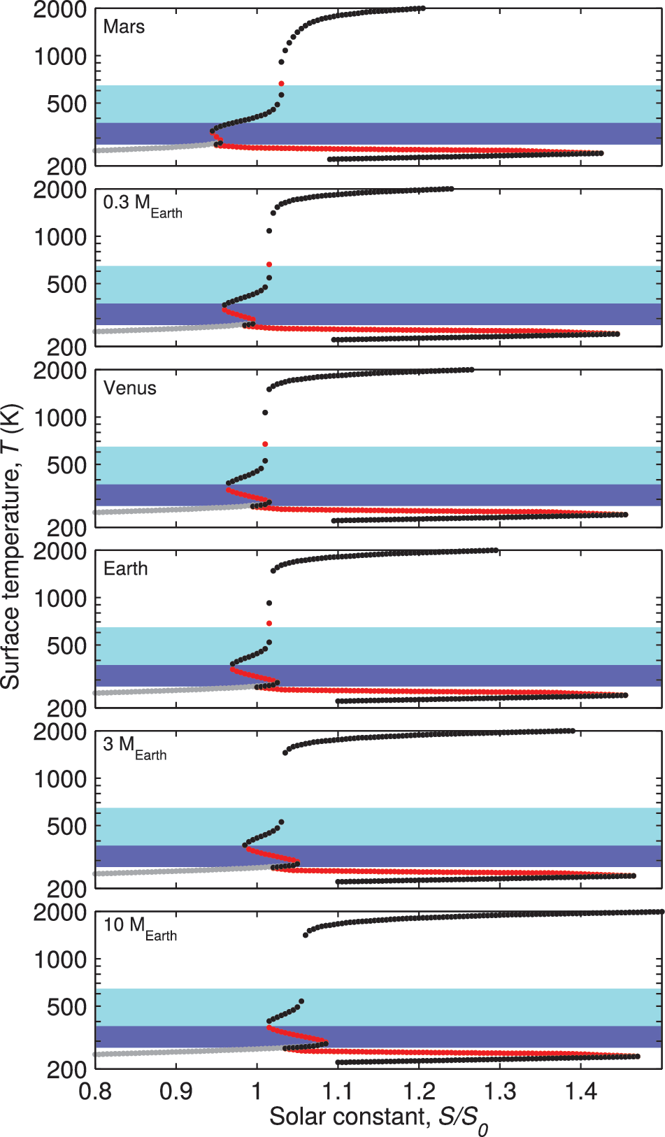
Comparing the outgoing thermal flux to the net solar flux scaled by an arbitrary solar constant, allowing for expansion in both cases, allows us to map the stable states for waterworld climates (Fig. 4). In addition to the quintic nonlinearity that exists in \documentclass{aastex}\usepackage{amsbsy}\usepackage{amsfonts}\usepackage{amssymb}\usepackage{bm}\usepackage{mathrsfs}\usepackage{pifont}\usepackage{stmaryrd}\usepackage{textcomp}\usepackage{portland, xspace}\usepackage{amsmath, amsxtra}\pagestyle{empty}\DeclareMathSizes{10}{9}{7}{6}\begin{document}$${ \cal F}$$ \end{document} , arising directly from the radiative transfer through the clear-sky atmosphere, there is a cubic nonlinearity introduced by ice–albedo feedback. The resulting function has a seventh-degree nonlinearity. Hence, there are four stable steady states, separated by three unstable steady states, which I will describe in turn.

FIG. 4.

Stable states of temperature (note log scale) for each planet as a function of solar constant. Black markers are stable steady states; red markers are unstable steady states. Gray markers are stable steady states when ice–albedo feedback has been omitted. Note that the lowest stable state would extend to arbitrarily low temperature, but my calculations cease at 220 K. Blue shaded areas are the liquid water region (273–647 K), with the darker areas being below 373 K.

The coldest stable steady state is global ice cover (“Snowball Earth”), with T _s⪅245 K, extending from arbitrarily low solar constant (not shown due to 220 K minimum temperature) to S/S ₀≈1.45. Next is a cold and damp state (270⪅T _s⪅290 K) with liquid water. For both these states, stability arises from the negative temperature feedback with outgoing thermal radiation; the atmosphere is optically thin to thermal radiation, so increasing surface temperature gives increasing thermal emission to space. The two states are separated by the positive ice–albedo feedback. The cold and damp state becomes unstable when the negative temperature feedback breaks down—that is, outgoing thermal radiation asymptotes to a constant. This bifurcation is typically thought of as the threshold for a runaway greenhouse (Nakajima et al., 1992; Goldblatt and Watson, 2012), when absorbed solar flux exceeds the limit on thermal emission. However, a complete runaway does not occur here, as there is an intermediate, hot and moist, stable state (350⪅T _s⪅550 K). The stability of this arises from a negative feedback between temperature and absorbed solar radiation; warming evaporates ocean and increases atmospheric mass, in turn increasing the amount of Rayleigh scattering such that less sunlight is absorbed. Only after the absorption of solar radiation asymptotes, when T _sx2A86;550 K, does the terminal runaway greenhouse occur. The final climate state is very hot and dry (typically T _sx2A86;900 K), above the critical point, so distinct liquid and vapor phases no longer exist. Stability arises from the reestablishment of a negative temperature feedback, with 4 μm emission from the atmosphere increasing with temperature.

Each stable steady state exists over some range in S/S ₀, the position and width of which depends on planet size (Fig. 5). The cold damp state exists at larger S/S ₀ and has a larger range on bigger planets. Similarly, snowball-like conditions can exist at higher S/S ₀ on bigger planets. The warm moist state has its base at higher S/S ₀ on bigger planets, but its warm edge has a minimum around Venus size. Likewise, the base of the hot dry state is minimal around Venus size.

FIG. 5.

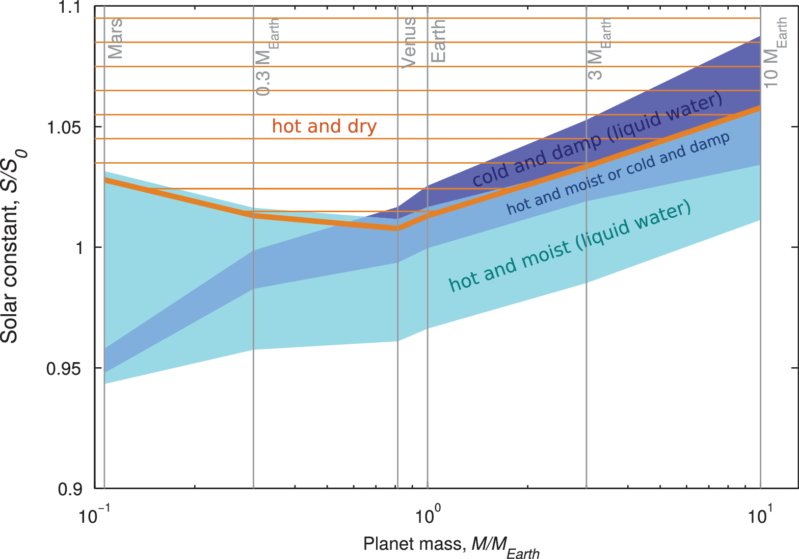
Stable climate states mapped as a function of planet mass. Blue shaded regions have liquid water: the darker area is where cold and damp climate is stable, the lighter area is where hot and moist climate is stable, and the intermediate shading is where both are stable. The orange hatched area bounded by a thick line is the stable region for very hot and dry climate. Completely ice-covered regime is stable everywhere (not shown).

A counter-intuitive feature is that cold and damp climate is often stable only at relatively high solar constants. This is a consequence of the existence of the ice–albedo feedback. If this is neglected (gray dots in Fig. 4), cold and damp conditions continue to arbitrarily low solar constant, making this state much broader than hot and moist conditions. Indeed, it is the hot moist state that is fundamentally narrow, depending on the Rayleigh scattering feedback, which necessarily is limited to a small region of flux space. That this has its base at a lower solar constant than cold damp conditions does not have any profound significance.

4. Discussion and Conclusions

I have shown that there are four distinct stable steady states for climate in pure water atmospheres. Three arise directly from the pure sky radiative transfer, with the fourth contributed by ice–albedo feedback. Only one of these, cold damp climate with 270⪅T _s⪅290 K, would universally be considered habitable, though liquid water will also exist in the hot moist state with 350⪅T _s⪅550 K.

The existence of the hot moist stable state is, to the best of my knowledge, a novel finding. From a theoretical point of view, it is interesting because it owes its existence to a negative feedback whereby increasing planetary temperature increases the thickness of the atmosphere and the increase in Rayleigh scattering, and therefore planetary albedo dominates.

Practically, if hot moist climate turns out to be a robust result in less-idealized atmospheres, it may be relevant to the evolution of Venus, the future of Earth, or similar planets. The hot water-rich atmosphere would allow rapid hydrogen escape, while the liquid ocean would mean that carbon could be sequestered in carbonates, not atmospheric CO₂. Forced by stellar evolution, the duration of this climate state would be hundreds of millions of years, which is sufficient for loss of an Earth ocean of water (Watson et al., 1984). Liquid water is the standard definition of habitability; hyperthermophiles could live at the surface, and temperate conditions would exist at altitude. After sufficient water was lost, the planet would transition to a Dune-like climate state (Herbert, 1965; Abe et al., 2011), which is also habitable and has a much higher runaway greenhouse threshold (Abe et al., 2011). This could add a billion years or more to the habitable period.

I did not consider clouds, partly for expedience [many model runs would have been needed (see Goldblatt and Zahnle, 2011), which would have been very costly] and partly to keep the focus on fundamental results arising from clear-sky radiative transfer. However, one must assess whether these results would be robust to contact with clouds. For temperate atmospheres, wide variation of clouds alters the stable state temperature but does not change the qualitative behavior (Goldblatt and Zahnle, 2011). However, with more complicated qualitative behavior here, one can have little certainty; a wide parameter space for clouds should be considered, but this has to be left for the future.

Accounting for expansion of the emitting and absorbing levels of runaway greenhouse atmospheres makes the threshold for a runaway greenhouse larger, especially for small planets, moving the inner edge of the habitable zone inward. Given the preferential affect on small planets, this changes the shape of the habitable zone with respect to planet mass.

One of the more curious features of these results is the very narrow habitable zone for pure water atmospheres. In the sense of proof by contradiction, this demonstrates the importance of noncondensible gas to stable climate. Adding bulk gas (e.g., ∼1 bar N₂) would markedly weaken the nonlinearity associated with increasing Rayleigh scattering as the atmosphere becomes thicker. It would also pressure-broaden the absorption lines of water, so the cold and damp stable state would extend to lower solar constants. Adding much more still might extend the habitable zone to higher temperatures by scattering away sunlight. Adding greenhouse gas (e.g., CO₂), especially in the presence of a background gas (Goldblatt et al., 2009b), can extend the habitable zone to lower temperatures. Our knowledge of the long-term carbon and nitrogen cycles is somewhat rudimentary for Earth and nonexistent for exotic planets. Given that these gasses are biologically controlled, habitability depends on inhabitance, and the width of the habitable zone is difficult to characterize.

Footnotes

Acknowledgments

Thanks to Brendan Byrne and Kevin Zahnle for comments on the manuscript. This work was funded by C.G.'s NSERC Discovery grant and by NASA Planetary Atmospheres grant NNX11AC95G.

References

Abe

and Matsui

(1988) Evolution of an impact generated H₂O–CO₂ atmosphere and formation of a hot proto-ocean on Earth. Journal of the Atmospheric Sciences, 45:3081–3101.

Abe

, Abe-Ouchi

, Sleep

N.H.

, and Zahnle

K.J.

(2011) Habitable zone limits for dry planets. Astrobiology, 11:443–460.

Goldblatt

and Watson

A.J.

(2012) The runaway greenhouse: implications for future climate change, geoengineering and planetary atmospheres. Philos Transact A Math Phys Eng Sci, 370:4197–4216.

Goldblatt

and Zahnle

K.J.

(2011) Clouds and the Faint Young Sun paradox. Climate of the Past, 7:203–220.

Goldblatt

, Claire

M.W.

, Lenton

T.M.

, Matthews

A.J.

, Watson

, and Zahnle

K.J.

(2009a) Nitrogen-enhanced greenhouse warming on early Earth. Nat Geosci, 2:891–896.

Goldblatt

, Lenton

T.M.

, and Watson

A.J.

(2009b) An evaluation of the longwave radiative transfer code used in the Met Office Unified Model. Quarterly Journal of the Royal Meteorological Society, 135:619–633.

Goldblatt

, Robinson

T.D.

, Zahnle

K.J.

, and Crisp

(2013) Low simulated radiation limit for runaway greenhouse climates. Nat Geosci, 6:661–667.

Herbert

(1965) Dune, Chilton Books, Philadelphia, PA.

Junglas

(2008) Implementing the IAPWS-95 standard in MATLAB. In Proceedings of the 15th International Conference on the Properties of Water and Steam, International Association for the Properties of Water and Steam, Berlin.

10.

Kasting

J.F.

(1988) Runaway and moist greenhouse atmospheres and the evolution of Earth and Venus. Icarus, 74:472–494.

11.

Kasting

J.F.

, Pollack

J.B.

, and Crisp

(1984) Effects of high CO₂ levels on surface temperature and atmospheric oxidation-state of the early Earth. J Atmos Chem, 1:403–428.

12.

Léger

, Selsis

, Sotin

, Guillot

, Despois

, Mawet

, Ollivier

, Labèque

, Valette

, Brachet

, Chazelas

, and Lammer

(2004) A new family of planets? “Ocean-planets.”. Icarus, 169:499–504.

13.

Meadows

V.S.

and Crisp

(1996) Ground-based near-infrared observations of the Venus nightside: the thermal structure and water abundance near the surface. J Geophys Res, 101:4595–4622.

14.

Nakajima

, Hayashi

Y.-Y.

, and Abe

(1992) A study of the “runaway greenhouse effect” with a one-dimensional radiative–convective model. Journal of the Atmospheric Sciences, 49:2256–2266.

15.

Pierrehumbert

R.T.

(2010) Principles of Planetary Climate, Cambridge University Press, Cambridge, UK.

16.

Pollack

J.B.

(1971) A nongrey calculation of the runaway greenhouse: implications for Venus' past and present. Icarus, 14:295–306.

17.

Raymond

S.N.

, Quinn

, and Lunine

J.I.

(2004) Making other Earths: dynamical simulations of terrestrial planet formation and water delivery. Icarus, 168:1–17.

18.

Rothman

L.S.

, Gordon

I.E.

, Barber

R.J.

, Dothe

, Gamache

R.R.

, Goldbman

, Perevalov

V.I.

, Tashkun

S.A.

, and Tennyson

(2010) HITEMP, the high-temperature molecular spectroscopic database. J Quant Spectrosc Radiat Transf, 111:2139–2150.

19.

Saltzman

(2002) Dynamical Paleoclimatology: Generalized Theory of Climate Change, Academic Press, San Diego, CA.

20.

Valencia

, O'Connell

R.J.

, and Sasselov

(2006) Internal structure of massive terrestrial planets. Icarus, 181:545–554.

21.

Wager

and Pruss

(2002) The IAPWS formulation 1995 for the thermodynamic properties of ordinary water substance for general and scientific use. J Phys Chem Ref Data, 31:387–535.

22.

Watson

A.J.

, Donahue

T.M.

, and Kuhn

W.R.

(1984) Temperatures in a runaway greenhouse on the evolving Venus: implications for water loss. Earth Planet Sci Lett, 68:1–6.

23.

Weiss

L.M.

and Marcy

G.W.

(2014) The mass-radius relation for 65 exoplanets smaller than 4 Earth radii. Astrophys J, 783, doi:10.1088/2041-8205/783/1/L6.