Automating X-ray Fluorescence Analysis for Rapid Astrobiology Surveys

Abstract

A new generation of planetary rover instruments, such as PIXL (Planetary Instrument for X-ray Lithochemistry) and SHERLOC (Scanning Habitable Environments with Raman Luminescence for Organics and Chemicals) selected for the Mars 2020 mission rover payload, aim to map mineralogical and elemental composition in situ at microscopic scales. These instruments will produce large spectral cubes with thousands of channels acquired over thousands of spatial locations, a large potential science yield limited mainly by the time required to acquire a measurement after placement. A secondary bottleneck also faces mission planners after downlink; analysts must interpret the complex data products quickly to inform tactical planning for the next command cycle. This study demonstrates operational approaches to overcome these bottlenecks by specialized early-stage science data processing. Onboard, simple real-time systems can perform a basic compositional assessment, recognizing specific features of interest and optimizing sensor integration time to characterize anomalies. On the ground, statistically motivated visualization can make raw uncalibrated data products more interpretable for tactical decision making. Techniques such as manifold dimensionality reduction can help operators comprehend large databases at a glance, identifying trends and anomalies in data. These onboard and ground-side analyses can complement a quantitative interpretation. We evaluate system performance for the case study of PIXL, an X-ray fluorescence spectrometer. Experiments on three representative samples demonstrate improved methods for onboard and ground-side automation and illustrate new astrobiological science capabilities unavailable in previous planetary instruments. Key Words: Dimensionality reduction—Planetary science—Visualization. Astrobiology 15, 961–976.

1. Introduction

T ime is a fundamental limiting resource for robotic planetary surveys. Historical missions such as Mars Pathfinder, Venus surface probes, and the Chang'e 3 Lunar expedition faced short lifetimes with few communications opportunities and few mission days to acquire data. Time bottlenecks also challenge longer-lived missions, such as the Mars rover Opportunity or the Mars Science Laboratory; upon reaching a new site of interest, they must quickly acquire a comprehensive dataset and form conclusive science interpretations so that the mission can progress to the next locale. In the future, astrobiology surveys will face even stricter constraints. A planned Mars 2020 surface rover would traverse kilometers of terrain while simultaneously identifying sites of interest and acquiring rock samples for later return to Earth (NASA Science Definition Team, 2014). The combination of kilometer-, meter-, and micro-scale survey with sample handling, extraction, and preservation makes efficient operations critical. Technologies to speed data acquisition and interpretation can expedite these core mission objectives and reduce risk. Moreover, accurate but fast analysis of each new locale will be vital for tactical decision making to maximize overall science yield over the finite mission lifetime.

This study focuses on two particularly challenging time bottlenecks. The first constraint is the instrument integration time. This is acute for sensors such as the Planetary Instrument for X-ray Lithochemistry (PIXL) or Scanning Habitable Environments with Raman Luminescence for Organics and Chemicals (SHERLOC) on board the Mars 2020 mission (Beegle et al., 2014; Allwood et al., 2015). These instruments aim to map mineralogical and elemental composition in situ at microscopic scales. They can produce large spectral cubes having thousands of channels and thousands of spatial locations. In large maps, each spectrum acquired by an instrument such as PIXL is likely to have a short integration time and consequently low signal to noise. Long integration times obtained by the summation of individual datapoints may be needed to quantify subtle compositional attributes, such as the minor and trace element abundance of textural features seen in element maps, with implications for returned sample quality. Examples include variations in elemental abundances bearing on the biogenicity of putative microbialites and the identification of minerals significant in terms of geochronology. The second bottleneck is the time to interpret downlinked data. Analysts' early tactical assessments inform instrument planning decisions about where the spacecraft should travel and what measurements it should attempt on the next command cycle. The rapid cadence of operations demands fast responses. However, manual grouping of similar spectra in large datasets is often not feasible within the time constraints of tactical mission operations. In addition, status quo approaches typically require days of processing, quality assurance, calibration, and assessment to achieve an authoritative analysis of complex datasets. This is challenging for instruments such as PIXL and SHERLOC and other mapping spectrometers with tens or hundreds of wavelength channels. These datasets defy easy visualization and typically reveal their best secrets only after days of analysis. It will therefore be critical to streamline an early tactical assessment of these datasets for optimal instrument planning.

This work demonstrates that automation can help address both bottlenecks. Figure 1 illustrates three timescales of analysis during operations decision making and the decisions relevant to each stage. This paper focuses on the two green boxes. First, we present onboard automated data analysis to improve acquisition speed and to reduce the number of command cycles needed to characterize a sample. Adaptive sampling uses simple spectral attributes to trigger longer integration times on microscale locations of interest. Such features are typically defined as a spectrum matching a desired compositional signature, anomalous compositions that differ from anything yet seen, or a rare and unexpected mineral whose presence is only hypothetical. Adapting integration time allows the instrument to find these “needles in a haystack” and focus a reserved portion of the acquisition time on these sites. Onboard analysis can also save command cycles by searching for a signature observed on a previous command cycle—essentially, returning to an area of interest with a placement accuracy exceeding the physical precision of the rover arm.

FIG. 1.

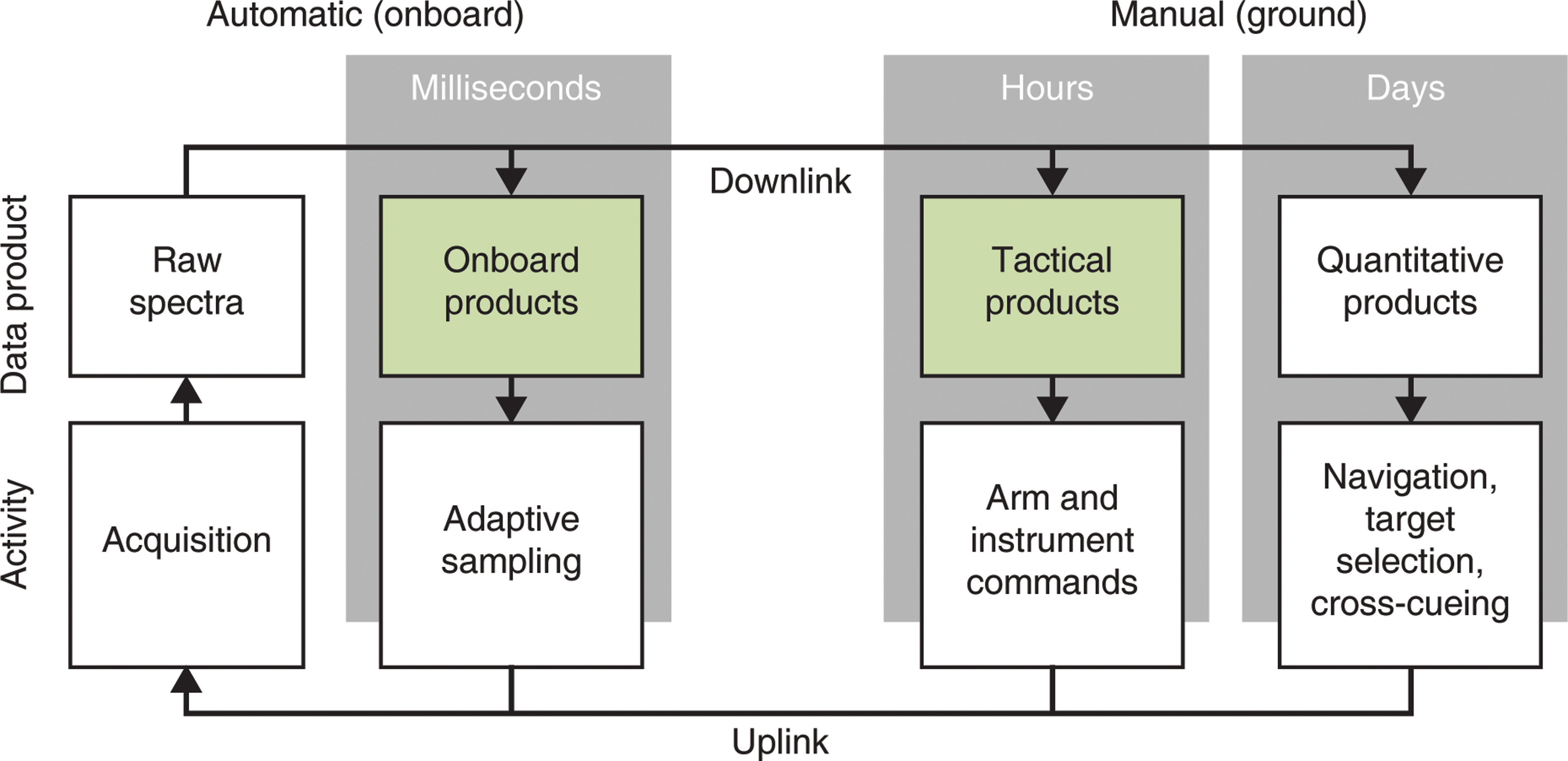
Three timescales on which instrument analysis occurs during remote astrobiology survey. This paper focuses on the two green boxes. (Color graphics available at www.liebertonline.com/ast)

Next, we address the analysis bottleneck with visualization methods that enable operators to identify outliers, form categorizations, and understand large quantities of spectral or image information at a glance. This allows analysts to partially assess data quality before a fully calibrated analysis is available. We focus on data-driven statistical methods, which apply readily to a wide range of products including visible/infrared spectra, X-ray fluorescence (XRF) spectra, neutron spectra, and radar data. Specifically, we apply principles of manifold dimensionality reduction, projecting measurements to points on the 2-D plane in such a way that similar spectra lie close together. The analyst can use this representation to immediately see trends, clusters, and outliers.

Dimensionality reduction has been applied to diverse fields including molecular biology and dynamical systems analysis (Gorban and Zinovyev, 2010), but there has been little attempt on planetary data.

As a case study, we consider XRF data from the breadboard version of PIXL. This is an appropriately stressing example, since data volumes are large (as many as 10⁴ datapoints per acquisition) and contain challenging structure on many scales. We assess different adaptive sampling criteria as well as linear and nonlinear dimensionality reduction techniques. Our study tests the following hypotheses:

(1) Onboard, adaptive sampling seeking novel composition provides a higher diversity of compositions than traditional “blind” data acquisition by evenly spaced transects and raster patterns; that is, it achieves a more diverse dataset in a shorter time.

(2) Onboard, adaptive sampling can reliably find specific spectra, overcoming expected instrument placement errors to enable same-cycle measurements of interesting locations.

(3) On the ground, purely statistical dimensionality reduction techniques reveal the most relevant compositional differences without the need for absolute calibration.

(4) On the ground, nonlinear dimensionality reduction strategies provide more faithful interpretations than linear methods; that is, they better capture the numerical structure in the original data product.

We evaluate these hypotheses for three representative PIXL datasets of varying complexity.

We begin by presenting the datasets and preprocessing common to all experiments. Next, we present the adaptive sampling approach and the result of several simulations that emulate mission data acquisition. The following section describes dimensionality reduction techniques for interpreting the data, applies a battery of candidate algorithms, and evaluates their efficacy with respect to geological accuracy and fidelity. Finally, we conclude by discussing the implications for operations design and the broader potential for other missions.

2. Data Acquisition and Reduction

We focus on PIXL, an XRF spectrometer designed to be mounted on a rover arm for interrogating rock outcrops (Lawrence et al., 2012; Allwood et al., 2015). PIXL emits a focused beam of X-rays onto the sample through a polycapillary from a distance of less than 5 cm. These interact with the sample to displace electrons from atoms' inner orbits, vacancies that are subsequently filled from outer shells. This emits X-rays of characteristic energies, which are sensed by a silicon drift detector producing distinctive fingerprints for each element. PIXL uses a source-ray focusing optic with very high spatial resolution (100 μm for the first breadboard instrument), actuated to acquire measurements in transects or grid patterns and generate fine-scale elemental maps. Each spectrum has 4096 distinct energy channels from 0 to 41 KeV.

We acquired three datasets of different sizes and complexities: “Troughite,” a living microbialite collected from standing water in the Mojave Desert (13,149 spectra, 15-second integrations); “Black Beauty,” a piece of NWA 7533, a martian meteorite paired with NWA 7034 (8,014 spectra, 30-second integrations); and “Shionoha,” a travertine, a carbonate precipitate collected from Shionoha hot springs in Japan (11,858 spectra, 16-second integrations). We mapped the cut and polished surface of each sample in a raster grid pattern using step sizes of approximately 100 microns. The samples show a wide range of structure and complexity. The Shionoha sample is a relatively simple compositional gradient, while the Troughite sample is a polymict of many diverse grains of different compositions. To facilitate a geological interpretation, we also acquired geological thin sections and photomicrographs of the Troughite and Shionoha samples, providing fine-scale petrological information including the mineralogy of grains and the distribution of cements. We co-registered these images using manual ground-control points to fit a simple affine transformation between the two frames. This provided a co-registration match with a root mean squared error of less than the PIXL beam footprint of 100 μm. We labeled the most obvious geological categories in the Troughite image: grains of quartz, feldspar, k-feldspar, carbonate, and iron oxides. This allowed us to correlate populations of spectra identified via dimensionality reduction with sample mineralogy and other features.

Figure 2 shows typical PIXL spectra from the Black Beauty sample. The raster image appears in the top panel in false color. The top panel highlights two different color-coded regions having distinctive compositions. These contain mean spectra plotted in the bottom. Peaks indicate the abundance of different chemical elements. Other features include a Bremsstrahlung signal (the large, flat continuum shape) and occasional false peaks due to scattering and diffraction effects. Our analysis first calculated descriptive intensity values using the energy channels of the dominant Kα1 peaks for Al, Si, Ca, S, P, Cl, Ti, K, Fe, Ba, Ce, Mn, Ga, Zr, Sr, and Y. More details on elemental line energies are found in the work of Bearden (1967).

FIG. 2.

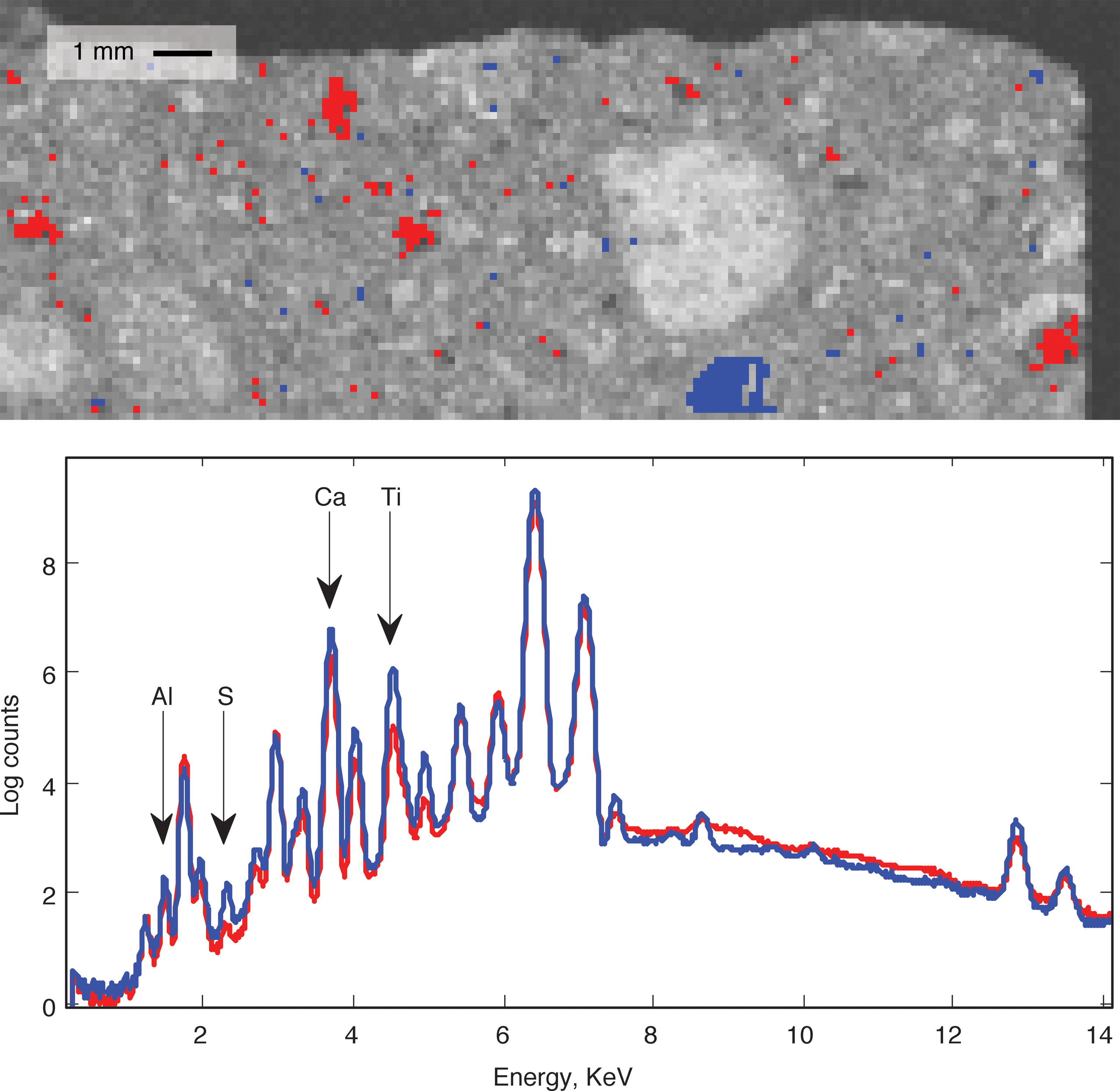
Top: The Black Beauty sample. Bright blue and red regions indicate materials of two distinctive compositions. Bottom: Mean spectrum of the blue and red regions. (Color graphics available at www.liebertonline.com/ast)

To isolate the X-ray counts from these elements, we first estimated the Bremsstrahlung background using the SNIP algorithm of Ryan et al. (1988; Van Grieken and Markowicz, 2001). This nonparametric estimator estimates the background by smoothing the peak-removed signal. We subtracted this background, integrated the remainder over the channels associated with each element, and normalized the result by its local background (Jenkins, 1995). The final normalization accounts for intensity differences due to matrix effects, sensor placement, and geometry. At low energies below about 3 keV, the background signal is close to zero, making the normalization unstable. Instead, we used the Bremsstrahlung signal at 3 keV as a proxy in these wavelengths. This was adequate for simple relative comparisons of line intensities, though a true quantitative evaluation might improve accuracy further by fitting the Bremsstrahlung signal with a parametric model. The result of preprocessing is a multichannel image of element intensities interpretable as a map. Figure 3 shows raster images acquired from Shionoha, Black Beauty, and Troughite samples. We show relative intensity of aluminum (red), calcium (green), and titanium (blue). Each spatial location is associated with a full spectrum of X-ray counts and a full vector of element intensities.

FIG. 3.

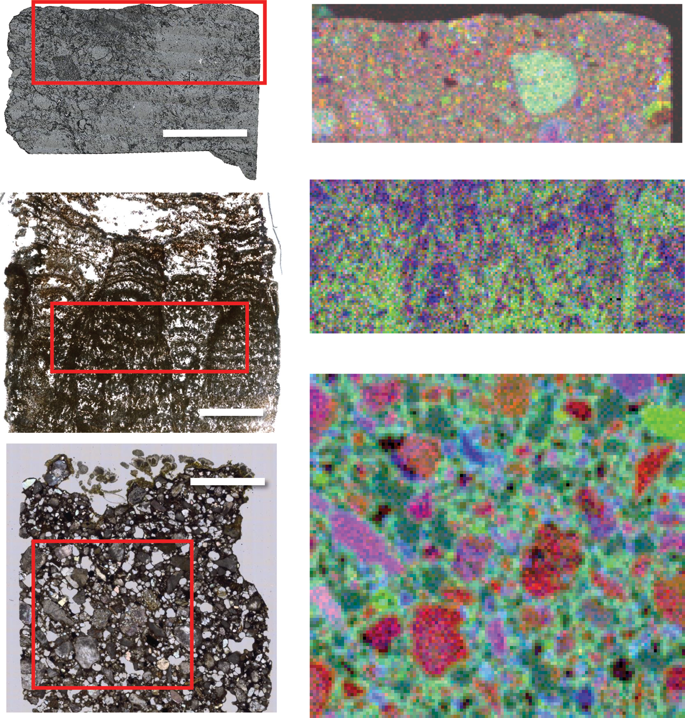
Left column, top to bottom: The Black Beauty, Shionoha, and Troughite samples. All scale bars are 5 mm. Red rectangles indicate the location of each PIXL raster. Right column, top to bottom: PIXL rasters showing three element channels in false color: Al (red), Ca (green), and Ti (blue). (Color graphics available at www.liebertonline.com/ast)

3. On Board: Adaptive Sampling

The PIXL instrument acquires data sequentially across transect and grid patterns, lingering at each location and integrating measurements over a period of seconds to minutes. Times as short as 5–10 s are used for a fast survey assessment to determine the bulk composition and recognize unit boundaries. Alternatively, long integrations of a minute or more provide very high-fidelity spectral data for deriving trace element compositions. It may be impractical to form complete images of high-fidelity spectra due to the time cost. This motivates adaptive sampling, in which the instrument performs an initial short survey measurement, autonomously analyzes the result, and makes an immediate decision “on the fly” about when to follow up with a long integration (Thompson et al., 2014). The net effect is to preferentially sample the geologically interesting data. Adaptive sampling can also be used to seek a very specific spectral signature observed on a previous command cycle. This can obtain long integrations from a site of interest, for example, using spectral feedback to place the instrument more accurately than the precision of the rover arm.

3.1. Adaptive sampling methods

The analysis begins with the initial preprocessing to reduce the spectrum to a vector of element line intensities. We then apply one of two adaptive sampling approaches. The first approach, a density-based method described previously by Thompson et al. (2014), maintains a library of all spectra collected during the transect. It acquires a new long-integration spectrum whenever the distance between the current spectrum and its closest long-dwell spectrum exceeds a threshold. Here, distance is defined as a weighted Euclidean distance between spectra. For a new spectrum u, library spectrum v, channel weights w, and threshold τ the rule is \documentclass{aastex}\usepackage{amsbsy}\usepackage{amsfonts}\usepackage{amssymb}\usepackage{bm}\usepackage{mathrsfs}\usepackage{pifont}\usepackage{stmaryrd}\usepackage{textcomp}\usepackage{portland, xspace}\usepackage{amsmath, amsxtra}\pagestyle{empty}\DeclareMathSizes{10}{9}{7}{6}\begin{document} \begin{align*}{ \rm trigger \ when} \ \exists \ v \ { \rm S}.{ \rm T}. \ d ( v , u ) > \tau \tag{1}\end{align*} \end{document} \documentclass{aastex}\usepackage{amsbsy}\usepackage{amsfonts}\usepackage{amssymb}\usepackage{bm}\usepackage{mathrsfs}\usepackage{pifont}\usepackage{stmaryrd}\usepackage{textcomp}\usepackage{portland, xspace}\usepackage{amsmath, amsxtra}\pagestyle{empty}\DeclareMathSizes{10}{9}{7}{6}\begin{document} \begin{align*} { \rm where } \ d ( u , v ) = \sqrt { \mathop \sum \limits_ { i = 0 } ^N \left( \frac { u_i - v_i } { w_i } \right) ^2 } \end{align*} \end{document}

The rule bounds the maximum distance between any measurement and the closest long-dwell spectrum, causing long integrations to spread evenly throughout the space of compositions. Channel weights control the relative influence of different lines and can be set according to the investigation objectives. Alternatively, an operator can treat all lines equally by setting w to their standard deviations. A total cap on the number of long-dwell spectra is imposed to enforce time limits; if this budget is reached, the system would forgo further long-dwell spectra. A typical example is a 2 h raster map with a budget of 20% of that time reserved for long-dwell spectra.

The second trigger criterion is an interval-based approach that defines value ranges for each element channel. An exclusive rule, used for finding anomalous compositions, triggers a long-dwell spectrum when the measurement exceeds this envelope in any channel. For an interval in channel i represented by the set Q_i , the rule is \documentclass{aastex}\usepackage{amsbsy}\usepackage{amsfonts}\usepackage{amssymb}\usepackage{bm}\usepackage{mathrsfs}\usepackage{pifont}\usepackage{stmaryrd}\usepackage{textcomp}\usepackage{portland, xspace}\usepackage{amsmath, amsxtra}\pagestyle{empty}\DeclareMathSizes{10}{9}{7}{6}\begin{document} \begin{align*}{ \rm trigger \ when} \ \exists i \ { \rm S}.{ \rm T}. u_i \,\notin\, Q_i \tag{2}\end{align*} \end{document}

Intervals could be given in intensity values, but this work defines Q in terms of standard deviations from the mean. For example, the interval Φ_i = [−3, 3] ensures that any outlier in channel i lying more than three standard deviations outside the mean triggers a long dwell. The mean and standard deviations are estimated directly from spectral data as the transect progresses. If the instrument can reliably return to a prior location along its transect, it would be desirable to accumulate statistics over the entire dataset and select outliers upon reaching the end. This would also allow the most significant outliers to be prioritized. However, thermal expansion of the arm upon reaching the end of the scan may prevent reliable return to a previous position within 100 μm. For generality, we will focus here on the most restrictive case where the instrument can only visit each point once.

One can also use intervals as an inclusive criterion for finding a specific signature of interest. This triggers when all channel values lie within prescribed ranges (i.e., a close match). \documentclass{aastex}\usepackage{amsbsy}\usepackage{amsfonts}\usepackage{amssymb}\usepackage{bm}\usepackage{mathrsfs}\usepackage{pifont}\usepackage{stmaryrd}\usepackage{textcomp}\usepackage{portland, xspace}\usepackage{amsmath, amsxtra}\pagestyle{empty}\DeclareMathSizes{10}{9}{7}{6}\begin{document} \begin{align*}{ \rm trigger \ when} \ u_i \in Q_i \forall i \tag{3}\end{align*} \end{document}

Together, these rules provide a rich palette of options for instrument operations. As a control, we also evaluate two non-adaptive rules: periodic sampling acquires data at regular intervals across the transect, with spacing appropriate to the total budget; and random sampling that allocates its prescribed number of samples randomly.

3.2. Adaptive sampling performance metrics

One important goal of adaptive sampling is to improve the diversity of long integrations. We quantify diversity using Shannon entropy (Cover and Thomas, 2012), which describes the amount of information contained in the set of long-dwell spectra. Shannon entropy is the foundation of experimental design criteria such as D-optimal design. We assume the intensities are independently distributed Gaussians, in which case the score is a differential entropy h: \documentclass{aastex}\usepackage{amsbsy}\usepackage{amsfonts}\usepackage{amssymb}\usepackage{bm}\usepackage{mathrsfs}\usepackage{pifont}\usepackage{stmaryrd}\usepackage{textcomp}\usepackage{portland, xspace}\usepackage{amsmath, amsxtra}\pagestyle{empty}\DeclareMathSizes{10}{9}{7}{6}\begin{document} \begin{align*}h = \mathop \sum \limits_i \frac { 1 } { 2 } \log \left( 2 \pi \sigma_i^2 \right) \tag { 4 } \end{align*} \end{document}

where \documentclass{aastex}\usepackage{amsbsy}\usepackage{amsfonts}\usepackage{amssymb}\usepackage{bm}\usepackage{mathrsfs}\usepackage{pifont}\usepackage{stmaryrd}\usepackage{textcomp}\usepackage{portland, xspace}\usepackage{amsmath, amsxtra}\pagestyle{empty}\DeclareMathSizes{10}{9}{7}{6}\begin{document}$$\sigma_i^2$$ \end{document} represents the variance of long-dwell values in channel i. Redundancy or repetitive data would reduce this score. This is a simplified form of the more general multivariate distribution having correlations across channels, where the differential entropy is proportional to the log determinant of the covariance matrix. The more general form might be a more accurate reflection of information content, but there are rarely more than a handful of long-dwell spectra, so its determinant calculation is unstable. We find that the isotropic case described above provides a good approximation and an effective metric for comparing the diversity of widely different datasets.

In this work, we evaluated diversity by simulating transects across each sample, one row at a time. The budget of long-dwell spectra was 20% of the traverse length. This is appropriate to balance survey and follow-up since the integration time of long-dwell spectra is often 5–10 times that of the short spectra. It also provided sufficient samples for data-driven adaptive methods to characterize the specimen. In a multiday operations scenario, operators could predict the values expected and tune performance with tighter interval criteria. Here, we erred on the side of conservatism and forced the adaptive system to recharacterize the sample tabula rasa with each transect. We applied adaptive sampling to each dataset, using distance thresholds of 4 standard deviations for both density and interval methods. This value was found experimentally to offer best performance across all datasets.

Apart from diversity, we considered a second performance measure to evaluate the system's potential to reliably return to a prior location. For any given spectrum, the distance to other locations in the sample (measured in channel intensity space) indicates whether that signature is unique enough to distinguish it. We calculate a noise-weighted distance in each channel using \documentclass{aastex}\usepackage{amsbsy}\usepackage{amsfonts}\usepackage{amssymb}\usepackage{bm}\usepackage{mathrsfs}\usepackage{pifont}\usepackage{stmaryrd}\usepackage{textcomp}\usepackage{portland, xspace}\usepackage{amsmath, amsxtra}\pagestyle{empty}\DeclareMathSizes{10}{9}{7}{6}\begin{document} \begin{align*}d ( u , v ) = \sqrt { \mathop \sum \limits_ { i = 0 } ^N \left( \frac { u_i - v_i } { \sigma_i } \right) ^2 } \tag { 5 } \end{align*} \end{document}

Here, σ_i is the standard deviation of noise in channel i (calculated from Poisson statistics). The smallest such value indicates the signal-to-background ratio presented by that unique spectral signature. However, we must also account for the fact that neighboring spatial locations are often similar enough to count as identical—it is usually acceptable to hit an immediate neighbor of the target. Consequently, we exclude a small local window of radius r from the nearest-neighbor search. This target size, which we set at 5, 10, 20, or 40 pixels, defines a neighborhood within which we hope to reacquire a long-dwell spectrum.

3.3. Adaptive sampling results

Figure 4 shows an example transect across the Black Beauty sample, with dots indicating locations selected for long integrations. As expected, the selected locations cluster mainly on small particles having distinctive composition or enrichment in one or more elements. The total budget of 28 is 20% of the total transect length. This is a particularly diverse sample with several small compositional anomalies along the transect. Most in situ samples would probably contain just one (or at most two) outlier locations.

FIG. 4.

A typical transect across the Black Beauty sample, using the interval-based method with a threshold of 3σ. Dots represent locations selected for long-dwell spectra. (Color graphics available at www.liebertonline.com/ast)

Figure 5 compares differential entropies for random sampling (R), periodic sampling (P), adaptive density-based sampling (AD), and adaptive interval-based sampling (AI). Larger differential entropy scores are better. The circles and lines represent means and standard deviations of the diversity score, with each row taken as a separate and independent trial. There is a wide spread of values across trials, reflecting varying diversity across each row of the raster. Even for very diverse samples, some transects are homogeneous—and adaptive sampling cannot change these scores. There is also a wide difference in magnitudes for different samples, reflecting the heterogeneity of the different specimens. Shionoha is the simplest, and even the best-performing trials have a low differential entropy. In contrast, even random sampling can achieve a very high information content when applied to the Troughite dataset. Both adaptive sampling methods outperform static and random approaches for every specimen (p < 0.001 for an unpaired t test). The Black Beauty dataset shows the largest benefit and the widest separation of adaptive and non-adaptive scores. This is consistent with the presence of many small grains that are difficult to find by chance.

FIG. 5.

Differential entropy, a measure of diversity, achieved by applying different sampling strategies to each specimen. Higher scores are better. “n” (at top) signifies the number of rows in the sample, with each row treated as a separate trial. R: random; P: periodic, regular spacing; AD: adaptive, density-based; AI: adaptive, interval-based. Circles and lines show data means and standard deviations, respectively. The system was permitted a number of long-dwell spectra equal to 20% of the total transect length.

Next, we calculated the fraction of pixels that could be reacquired by their spectral signature—in other words, the fraction of pixels with a spectrum that differed from others outside its neighborhood by at least 3σ. Table 1 shows four different target size radii. Values are consistent with the first test: the Shionoha sample has the most homogeneous background, and just a few spectra can be reliably reacquired. In contrast, large fractions of the Troughite sample are unique and can be reacquired to high precision.

Table 1.

Fraction of Pixel Locations That Are Reachable (Signal to Background >3), for Different Target Sizes

Target size (pixels)	Black Beauty	Troughite	Shionoha
5	0.1643	0.8594	0.0184
10	0.1884	0.8862	0.0212
20	0.2329	0.9091	0.0245
40	0.2746	0.9480	0.0343

Figure 6 shows the nearest-neighbor distances as a map, calculated for target size 10. The signal-to-background score indicates locations that could be reliably targeted by using a spectral signature technique. Note that small, distinctive features are quite easy to reacquire, while the centers of large homogeneous areas are more difficult to hit precisely. This offers a very conservative performance assessment; an instrument might still be able to hit these larger targets through a combination of looser positioning requirements and careful selection of a transect direction to maximize target contrast.

FIG. 6.

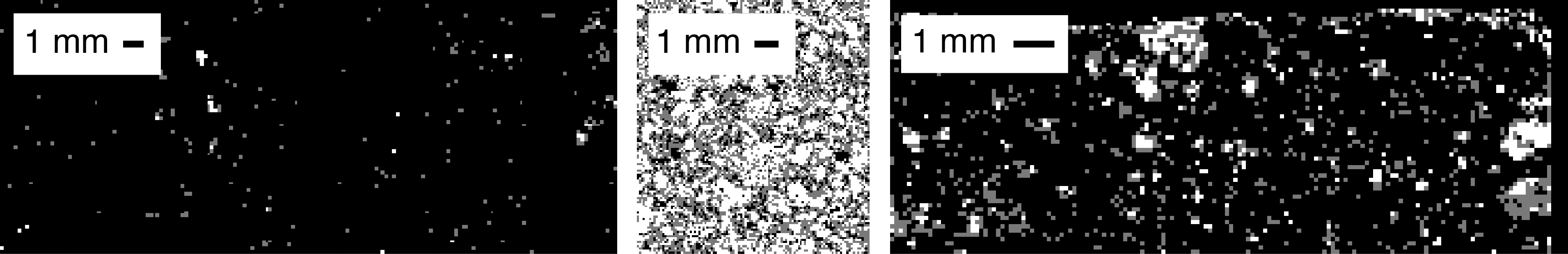
Signal-to-background score for each specimen, for reacquiring spectra inside a 5-pixel neighborhood. Gray pixels have scores greater than 3; white pixels are greater than 6. Specimens (left to right): Black Beauty, Troughite, and Shionoha.

3.4. Discussion

Experiments in adaptive sampling demonstrate significant improvements in sample diversity for survey transects, corroborating prior work detailed by Thompson et al. (2013). Both adaptive sampling approaches consistently improve the result achieved by periodic sampling. Neither the interval-based nor the density-based approach significantly outperforms the other. However, the implementation simplicity of the interval-based method, combined with its capability of re-acquiring prior spectra, makes it a compelling option.

These experiments show that many, but not all, areas of the specimens have signatures that are unique enough to reacquire based on spectral content alone. These features, which can be acquired, are exactly the small, unique areas that would be difficult to find when using conventional techniques. Consequently, adaptive sampling could play an important role in operations as operators attempt to measure microscale features accurately. Regardless, it would also be useful to pair these approaches with visually guided sampling to ensure that all areas of the sample are reachable.

4. On Ground: Visualization

This section focuses on the second challenge of rapid ground-side data analysis, with several algorithms designed to assist interpretation of downlinked data. Figures 2 and 3 illustrate challenges in interpreting these datasets. Neither the image representation nor the spectrum is sufficient: RGB color images can show many datapoints at once but only portray three spectral channels at a time, while the spectrum shows all spectral channels but can only portray a single point location. One can explore the data more fully by cycling the raster image through multiple color mappings, but this is impractical for more than a handful of combinations and relies on fallible human memory to synthesize the information. It is also easy to overlook subtle artifacts and measurement errors in single spectra. Such problems in data quality are expected when exploring poorly characterized remote environments. Together, these challenges motivate a new visualization approach to improve the reliability and reduce cognitive load on instrument command decisions.

Dimensionality reduction is a well-studied technique for visualizing complex datasets. It aims to represent high-dimensional datasets by using compressed versions that capture all the relevant structure. For PIXL data, this means projecting thousands of 4096-dimensional spectra onto a 2-D plane while preserving the similarity of neighbor relationships. We desire that this projection be interpretable, emphasizing the key physical distinctions relevant to the investigation. The visualization should reveal all relevant variance, without excluding phenomena or being dominated by any one trend. The visualization should also be faithful to the original, representing the underlying numerical data with minimal distortion. Finally, we desire that it transparently handle many different, diverse targets. This is critical because the visualization is most likely to be used in a rapid first analysis of data and operators may not know the feature's targets or data quality in advance. To our knowledge, ours is the first research to investigate the issue of statistical data visualization methods specifically for science decision making during field campaigns. The planetary domain is challenging since the environment is highly unconstrained; instrument artifacts and noise routinely exceed that in conventional, sanitized benchmark datasets used for developing dimensionality reduction methods.

4.1. Dimensionality reduction methods

We consider several linear and nonlinear dimensionality reduction methods, beginning each analysis with the intensity vector x ∈ \documentclass{aastex}\usepackage{amsbsy}\usepackage{amsfonts}\usepackage{amssymb}\usepackage{bm}\usepackage{mathrsfs}\usepackage{pifont}\usepackage{stmaryrd}\usepackage{textcomp}\usepackage{portland, xspace}\usepackage{amsmath, amsxtra}\pagestyle{empty}\DeclareMathSizes{10}{9}{7}{6}\begin{document}$${\mathbb R}$$ \end{document} ⁿ having one entry in x for each Kα1 line. We seek a mapping f (x) = x′ : \documentclass{aastex}\usepackage{amsbsy}\usepackage{amsfonts}\usepackage{amssymb}\usepackage{bm}\usepackage{mathrsfs}\usepackage{pifont}\usepackage{stmaryrd}\usepackage{textcomp}\usepackage{portland, xspace}\usepackage{amsmath, amsxtra}\pagestyle{empty}\DeclareMathSizes{10}{9}{7}{6}\begin{document}$${\mathbb R}$$ \end{document} ⁿ ↦ \documentclass{aastex}\usepackage{amsbsy}\usepackage{amsfonts}\usepackage{amssymb}\usepackage{bm}\usepackage{mathrsfs}\usepackage{pifont}\usepackage{stmaryrd}\usepackage{textcomp}\usepackage{portland, xspace}\usepackage{amsmath, amsxtra}\pagestyle{empty}\DeclareMathSizes{10}{9}{7}{6}\begin{document}$${\mathbb R}$$ \end{document} ² transforming this vector of normalized line intensities to a 2-D ordered pair representing the row and column position in the visual map.

4.1.1. Principal component analysis (PCA)

Dimensionality reduction algorithms are broadly grouped into linear and nonlinear techniques. Classical principal component analysis (PCA; Shlens, 2005) finds a linear projection of the data onto a new orthonormal basis: a low-dimensional subspace to maximize the variance of the data. PCA was applied to XRF images over a decade ago in work by Vogt et al. (2003) and has become common for XRF analysis. One first centers the data so that \documentclass{aastex}\usepackage{amsbsy}\usepackage{amsfonts}\usepackage{amssymb}\usepackage{bm}\usepackage{mathrsfs}\usepackage{pifont}\usepackage{stmaryrd}\usepackage{textcomp}\usepackage{portland, xspace}\usepackage{amsmath, amsxtra}\pagestyle{empty}\DeclareMathSizes{10}{9}{7}{6}\begin{document}$$\left( \sum \nolimits_{i = 0}^n x^i = 0 \right)$$ \end{document} and then diagonalizes the covariance matrix: \documentclass{aastex}\usepackage{amsbsy}\usepackage{amsfonts}\usepackage{amssymb}\usepackage{bm}\usepackage{mathrsfs}\usepackage{pifont}\usepackage{stmaryrd}\usepackage{textcomp}\usepackage{portland, xspace}\usepackage{amsmath, amsxtra}\pagestyle{empty}\DeclareMathSizes{10}{9}{7}{6}\begin{document} \begin{align*}A = \frac { 1 } { n } \mathop \sum \limits_ { i = 1 } ^n x_ix_i^T \tag { 6 } \end{align*} \end{document}

and the solution is obtained by solving the eigenvalue equation, \documentclass{aastex}\usepackage{amsbsy}\usepackage{amsfonts}\usepackage{amssymb}\usepackage{bm}\usepackage{mathrsfs}\usepackage{pifont}\usepackage{stmaryrd}\usepackage{textcomp}\usepackage{portland, xspace}\usepackage{amsmath, amsxtra}\pagestyle{empty}\DeclareMathSizes{10}{9}{7}{6}\begin{document} \begin{align*}\lambda v = Av \tag{7}\end{align*} \end{document}

for eigenvalues λ ≥ 0 and v ∈ \documentclass{aastex}\usepackage{amsbsy}\usepackage{amsfonts}\usepackage{amssymb}\usepackage{bm}\usepackage{mathrsfs}\usepackage{pifont}\usepackage{stmaryrd}\usepackage{textcomp}\usepackage{portland, xspace}\usepackage{amsmath, amsxtra}\pagestyle{empty}\DeclareMathSizes{10}{9}{7}{6}\begin{document}$${\mathbb R}$$ \end{document} ⁿ. All the solutions v then lie in the span x ₁, x ₂ … x_n . The eigenvectors associated with the top eigenvalues become the new 2-D basis.

We follow the standard practice of using PCA as a preprocessing step to reduce noise and improve the computational complexity of other methods. When used in this way, we set the number of target dimensions to explain 99.999% of the data variance. This rule produces datasets with 3, 5, and 6 dimensions for the Shionoha, Black Beauty, and Troughite samples, respectively. We also evaluate the effect of a standardization transformation, following the strategy of Boardman and Kruse (2011) and further dividing all dimensions by the square root of their eigenvalues so that they had unit variance. This prevents a single strong element, or collection of correlated elements, from dominating the feature vector. Our evaluation will consider both standardized and nonstandardized preprocessing.

4.1.2. Factor analysis (FA) and probabilistic principal component analysis (PPCA)

PCA uses only second-order statistics, which is suboptimal if the data is not Gaussian-distributed. This is typical of PIXL data, which can contain linear trends and extruded, non-Gaussian clouds corresponding to compositional gradients. Some other linear techniques are free from the Gaussian assumption. Factor analysis (FA) (Bartholomew, 1987) posits a linear combination of bases perturbed by Gaussian noise ∈: \documentclass{aastex}\usepackage{amsbsy}\usepackage{amsfonts}\usepackage{amssymb}\usepackage{bm}\usepackage{mathrsfs}\usepackage{pifont}\usepackage{stmaryrd}\usepackage{textcomp}\usepackage{portland, xspace}\usepackage{amsmath, amsxtra}\pagestyle{empty}\DeclareMathSizes{10}{9}{7}{6}\begin{document} \begin{align*}x = W{x{\prime}} + \mu + \in \tag{8}\end{align*} \end{document}

Constraining the error ∈ to be a Gaussian with diagonal covariance N (0, ψ) means observations are distributed according to \documentclass{aastex}\usepackage{amsbsy}\usepackage{amsfonts}\usepackage{amssymb}\usepackage{bm}\usepackage{mathrsfs}\usepackage{pifont}\usepackage{stmaryrd}\usepackage{textcomp}\usepackage{portland, xspace}\usepackage{amsmath, amsxtra}\pagestyle{empty}\DeclareMathSizes{10}{9}{7}{6}\begin{document} \begin{align*}x \,\sim \,N \left( \mu , WW^T + \Psi \right) \tag{9}\end{align*} \end{document}

The observed variables x are conditionally independent given the latent variables, which are estimated via expectation maximization. Alternatively, positing a Gaussian prior distribution over latent variables x′ permits a closed-form solution leading to an algorithm commonly known as probabilistic principal component analysis (PPCA) (Tipping and Bishop, 1999).

4.1.3. Kernel principal component analysis (KPCA)

Another important group of projections involve nonlinear transformations. Here, there are dozens of options, so we focus for this study on well-known algorithms representing distinctly different methodologies. Kernel principal component analysis, or KPCA (Schölkopf et al., 1997), maps the data into a latent feature space φ(x) and there performs a linear dimensionality reduction. The result is to create a nonlinear mapping from x ↦ x′. To evaluate the projection for the j ^th component, written x′_j, one uses \documentclass{aastex}\usepackage{amsbsy}\usepackage{amsfonts}\usepackage{amssymb}\usepackage{bm}\usepackage{mathrsfs}\usepackage{pifont}\usepackage{stmaryrd}\usepackage{textcomp}\usepackage{portland, xspace}\usepackage{amsmath, amsxtra}\pagestyle{empty}\DeclareMathSizes{10}{9}{7}{6}\begin{document} \begin{align*}x_i{{ \prime}} = \left( \mathop \sum \limits_{i = 1}^n \alpha_i^k \phi ( x_i ) \right) ^T \phi ( x ) \tag{10}\end{align*} \end{document}

Solving for optimal values α involves an eigensystem based on the matrix of inner products 〈φ(x_n ), φ(x_n )〉. Since the actual coordinates of φ(x) are never used directly, the latent space can have very high dimensionality provided its inner products are still tractable. Here, we define the inner product as the product of Gaussian kernel functions, leading to an elegant closed-form solution. The bandwidth of the Gaussian kernel is an unknown parameter, so we perform a grid search over multiple bandwidths and (conservatively) use the performance corresponding to the best result.

4.1.4. Fast maximum variance unfolding (FMVU)

Another method based on local distances is fast maximum variance unfolding (FMVU) (Shlens, 2005); this optimizes a semidefinite programming problem that maximized the overall variance of projected data while preserving local distances. The FMVU procedure considers local distances within a neighborhood whose size is a free parameter; we select it using a grid search in this study.

4.1.5. Locally linear embedding (LLE)

Dimensionality reduction methods require that the intrinsic dimensionality of the data be low, so that the (noise-free) data lies on a surface embedded in the high-dimensional space. Locally linear embedding (LLE) (Roweis and Saul, 2000) builds on this intuition, seeking projections that preserve the local geometry of the manifold. LLE assumes that each datapoint lies on a low-dimensional hyperplane in a local neighborhood of k nearest neighbors. It finds the set of local weights of neighboring points to reconstruct each high-dimensional datum in the least-squares sense. It then fixes this weight matrix and solves for the low-dimensional representation that optimizes the reconstruction error—tantamount to an eigensystem with a closed-form solution. The number of neighbors k is set with a grid search.

4.1.6. Laplacian eigenmaps (LEM)

A contrasting approach is to build a graph structure for the data cloud and then identify a projection that preserves this connectivity. The Laplacian eigenmaps (LEM) algorithm (Belkin and Niyogi, 2003) starts with a graph of locally connected neighborhoods. It uses the n × n graph Laplacian matrix L, tantamount to a matrix representation of a graph with n nodes ν.

The Laplacian matrix represents each point's connections in this graph structure using \documentclass{aastex}\usepackage{amsbsy}\usepackage{amsfonts}\usepackage{amssymb}\usepackage{bm}\usepackage{mathrsfs}\usepackage{pifont}\usepackage{stmaryrd}\usepackage{textcomp}\usepackage{portland, xspace}\usepackage{amsmath, amsxtra}\pagestyle{empty}\DeclareMathSizes{10}{9}{7}{6}\begin{document} \begin{align*}L_{i , j} = \begin{cases}{ \rm deg} ( v_i ) \qquad { \rm if} \ i = j \\ - 1 \qquad \; \quad { \rm if} \ i \neq j \ { \rm and \ adj} ( v_i , v_j ) \\ 0 \qquad \qquad \; { \rm otherwise}\end{cases} \tag{11}\end{align*} \end{document}

where adj(ν _i , ν _j ) represents adjacency and deg(ν _i ) represents degree. The Laplacian can be interpreted as the difference of a diagonal weight matrix D summing the rows of a connectivity matrix W, W_i,j ∈ {0,1}, such that L = D − W is positive definite. LEM identifies top eigenvalues λ and eigenvectors f of the system \documentclass{aastex}\usepackage{amsbsy}\usepackage{amsfonts}\usepackage{amssymb}\usepackage{bm}\usepackage{mathrsfs}\usepackage{pifont}\usepackage{stmaryrd}\usepackage{textcomp}\usepackage{portland, xspace}\usepackage{amsmath, amsxtra}\pagestyle{empty}\DeclareMathSizes{10}{9}{7}{6}\begin{document} \begin{align*}Lf = \lambda Df \tag{12}\end{align*} \end{document}

The f vectors for the top two eigenvalues became the horizontal and vertical coordinates of the projected dataset. This is the embedding that best represents the connectivity relationships in the original graph. The number of neighbors included in the neighborhood graph is selected by using a grid search.

4.1.7. t-distributed stochastic neighborhood embedding (t-SNE)

Finally, we also consider stochastic neighborhood embedding (SNE) (Hinton and Roweis, 2002). In SNE, the high-dimensional Euclidean distances between points were first converted into p_i|j , the asymmetric conditional probability that the datapoint x_i would pick x_j as its neighbor, proportional to their Gaussian densities centered at x_i . With the same idea, in the low-dimensional space, SNE models the similarities of projected points x′_i and x′_j by the conditional probabilities. The objective is to match these distributions, typically achieved by minimizing the natural cost function KL-divergence (Shlens, 2014) over all datapoints. In this work, we use a variant based on the Student t distribution known as t-distributed stochastic neighborhood embedding (t-SNE) (Van der Maaten and Hinton, 2008). This allows dissimilar objects to be modeled far apart in the projected visualization.

Together, these methods constitute a diverse selection of density-, distance-, and topology-based approaches. The input values to all algorithms are normalized intensities. We considered further standardizing the variables by transforming them to have standard deviation one and mean zero, but since the majority of dimensions were not relevant, this increased the effect of noise and ultimately harmed most methods' performance. We report the normalized values here.

4.2. Dimensionality reduction performance metrics

We evaluate each method with two criteria. First, we measure the fidelity of the reduced representation, that is, the degree to which it captures the local structure in the raw dataset. The agreement rate metric (ARM) is a score for assessing dimensionality reduction (Akkucuk, 2004) defined as the fraction of nearest-neighbor relationships preserved in the low-dimensional representation: \documentclass{aastex}\usepackage{amsbsy}\usepackage{amsfonts}\usepackage{amssymb}\usepackage{bm}\usepackage{mathrsfs}\usepackage{pifont}\usepackage{stmaryrd}\usepackage{textcomp}\usepackage{portland, xspace}\usepackage{amsmath, amsxtra}\pagestyle{empty}\DeclareMathSizes{10}{9}{7}{6}\begin{document} \begin{align*} { ARM } = \frac { 1 } { kn } \mathop \sum \limits_ { i = 1 } ^n a_i \tag { 13 } \end{align*} \end{document}

Where a_i is the number of neighbors preserved in the low-dimensional projection of point i, n is the dataset cardinality, and k is the size of the local neighborhood. The score ranges from zero (no alignment) to one (perfect fidelity). In principle, it depends on the value of k, but in practice we found the behavior of the ARM scores was stable across a wide range of different values. We set k = 12 for these experiments, which yielded an informative breadth of performance scores while covering the smallest geological features (which could have as few as a dozen pixels). We use a kd-tree structure to search efficiently for nearest neighbors (Press et al., 2007).

Our second score evaluates classification accuracy using the standard nearest-neighbor classifier (Bishop, 2006). The classification score indicates how well the projected representation emphasizes petrological categories. The classifier relies on a ground-truth petrological interpretation, so we only perform this evaluation for the Troughite sample with co-registered optical microscopy. We split the dataset into training and testing halves, and for each datapoint of the testing spectrum, calculate a predicted class ĉ_i using \documentclass{aastex}\usepackage{amsbsy}\usepackage{amsfonts}\usepackage{amssymb}\usepackage{bm}\usepackage{mathrsfs}\usepackage{pifont}\usepackage{stmaryrd}\usepackage{textcomp}\usepackage{portland, xspace}\usepackage{amsmath, amsxtra}\pagestyle{empty}\DeclareMathSizes{10}{9}{7}{6}\begin{document} \begin{align*}\hat{c}_i = \arg { \rm max}_{{ \hat{c}_i}} \mathop \sum \limits_{{ \hat{c}_j} \in N_i} I ( c_j , \hat{c}_i ) \tag{14}\end{align*} \end{document}

Here, N_i is the local neighborhood of k training points nearest to point i, and I is the indicator function that evaluates to 1 if the predicted class ĉ_i is equal to c_j . We perform 20-fold cross validation, cycling through 20 held-out testing sets to estimate the error on a novel dataset. The nearest-neighbor classifier has been used previously in dimensionality reduction experiments (Van der Maaten and Hinton, 2008). It is free of parametric modeling assumptions about the form of the data and approaches the best-achievable theoretical performance for very dense datasets. Using a single nearest neighbor, rather than an ensemble of k neighbors, helps the classification score reflect the fine local structure as described in Van der Maaten et al. (2009).

Finally, we manually select three regions in the Black Beauty sample with distinctive compositions: enhancements in Ca, Ti, and Al corresponding to the red, green, and blue regions in Fig. 8. Tracing these spectra to each of the point clouds reveals the planar projections of different compositional units. Ideally, each unit should be compact, contiguous, and well-separated from the others.

4.3. Dimensionality reduction results

Figure 7 shows eigenvalues, in descending order, for the principal components of each dataset. Magnitudes are relative to the maximum eigenvalue on a logarithmic scale. The rate of decay shows the variance captured by each subsequent dimension, and the slope indicates the complexity of the dataset. Both Troughite and Black Beauty samples are complex, with variance along many independent dimensions. This agrees with the interpretation of these samples as polymicts of many different materials. In contrast, the Shionoha sample is relatively simple, exhibiting a much faster eigenvalue decay and just a few salient dimensions. This is characteristic of a single compositional unit with varying degrees of alteration.

FIG. 7.

Eigenvalues, relative to the maximum, for principal components of each sample. (Color graphics available at www.liebertonline.com/ast)

Figure 8 shows example projections applying each of the eight methods to the Black Beauty sample. The colored dots below show the groups' projections in the point cloud. In each case, we have cropped the point cloud to show the main body of the distribution. All methods generally do a good job of separating the three classes. PCA proves generally stable, producing point clouds that approximate a Gaussian distribution: a dense concentration of points in the center and a scattered spread of outliers at the periphery. The top row shows LLE and linear approaches, all of which resemble traditional PCA. FA is stable only when the raw nonstandardized data is used and generally fails to outperform classical PCA. Typical results from PPCA and LLE provide little or no benefit over PCA.

FIG. 8.

Projections of the Black Beauty spectra, with labels for three salient constituents of Fig. 2. Blue: enhanced Al. Green: enhanced Ti. Red: enhanced Ca. (Color graphics available at www.liebertonline.com/ast)

Nonlinear methods show more variability. KPCA produces cartoid structures with highly concentrated central regions and compositional units distributed on the periphery. LEM typically produces long filamentary structures. FMVU resulted in more uniform but disorganized clouds. Of all the methods, its features were least well-localized. Qualitatively, t-SNE is the top performer; it best combines an informative structure (filling the whole 2-D plane) with well-localized, compact, and separated features. The only obvious disadvantage to t-SNE is that it tends to fill the entire plane uniformly, reducing the visual salience of extreme outliers. For identifying outliers and endmembers, a linear projection like classical PCA may be more desirable.

Tables 2 and 3 show performance scores for all samples and visualization methods. The standardization gives no quantitative benefit to ARM or classification scores. ARM values vary widely, though algorithms' relative performance is consistent. Neither the linear nor nonlinear categories offer a uniform advantage, and performance depends entirely on the specific algorithm. Classical PCA offers very solid performance on all samples, outperforming many of the more sophisticated nonlinear and linear approaches. However, the top nonlinear algorithms perform best overall. The graph-based LEM and LLE strategies perform very well on raw data, with excellent ARM scores and classification accuracies of 93.5% and 92.5%, respectively. Classical Multidimensional Scaling (MDS), PCA, and PPCA score in similar ranges. t-SNE performs best overall, with superior ARM scores on five of six cases and superior classification scores. It achieves a total classification accuracy of 98.4, which is near perfect, signifying that the distinct geological groups identified in the image all fall into compact clusters in the t-SNE plot.

Table 2.

ARM and Classification Performance, Standardized Datasets

	Agreement rate metric			k-nn
	Black Beauty	Troughite	Shionoha	Troughite
Linear
FA	0.031	0.212	0.160	0.874
PPCA	0.038	0.196	0.235	0.923
PCA	0.059	0.070	0.241	0.733
Nonlinear
MDS	0.059	0.070	0.241	0.728
LEM	0.048	0.218	0.302	0.919
FMVU	0.029	0.068	0.196	0.884
LLE	0.051	0.218	0.279	0.887
KPCA	0.040	0.287	0.246	0.772
TSNE	0.133	0.440	0.245	0.989

Table 3.

ARM and Classification Performance, Nonstandardized Datasets

	Agreement rate metric			k-nn
	Black Beauty	Troughite	Shionoha	Troughite
Linear
FA	0.455	0.251	0.170	0.842
PPCA	0.478	0.296	0.352	0.939
PCA	0.488	0.321	0.439	0.933
Nonlinear
MDS	0.488	0.321	0.439	0.933
LEM	0.177	0.335	0.272	0.935
FMVU	0.118	0.116	0.238	0.858
LLE	0.468	0.341	0.437	0.925
KPCA	0.275	0.272	0.362	0.650
TSNE	0.523	0.633	0.628	0.984

Next, the projections for the Black Beauty and Shionoha samples demonstrate their value for finding spectral endmembers. Figure 9 shows the procedure, illustrated with intensities normalized using the Silicon Kα1 line (an alternative normalization strategy that yields similar results). The Black Beauty sample appears in the left column, and the Shionoha sample in the right. First, an analyst manually selects the extrema of the point cloud (top row). These points are mapped back into the original image coordinates (middle row). They are then used to extract average spectra (bottom row). The four endmember regions selected in Black Beauty correspond to compact regions with distinct spectra. The green endmember is an obvious numerical outlier due to high Ti enrichment. The blue endmember is enriched in K, red and yellow in Fe. The Shionoha spectra show much subtler differences, with minor changes in the abundance of Cl (originating in the epoxy used in the preparation of the thin section), Ca, and Fe in each of three endmembers. The blue versus green axis reflects the amount of Fe that is present, while the red axis is related to the quantity of Cl. Many of these regions subtend very small clusters containing 10 or fewer pixels. This makes them difficult to identify in the image maps alone. Nevertheless, the fact that they do form contiguous units corroborates an interpretation as real physical outliers, rather than (for example) artifacts.

FIG. 9.

End-member analysis using PCA. Top row: Point clouds for the samples Black Beauty (left) and Shionoha (right). Colored regions are manual labels ascribed arbitrarily to different extrema in the point cloud. Center row: The locations of the regions after back-projection onto the sample surface. Bottom row: The mean spectra corresponding to each image region. (Color graphics available at www.liebertonline.com/ast)

While PCA is useful to identify key compositional gradients, many different spectral distinctions are buried in the central concentration of points. Consequently, it does not necessarily show all the unique compositional units “at a glance.” However, the nonlinear method of t-SNE serves this objective well. We use it to fully interpret the t-SNE projection for the Troughite sample in Fig. 10. We manually color the scatterplot of Si-normalized data, highlighting clusters corresponding to different compositional units. Grains with novel compositions are easy to overlook in a brute-force inspection but are immediately evident in the t-SNE projection since the spectra appear as isolated clusters.

FIG. 10.

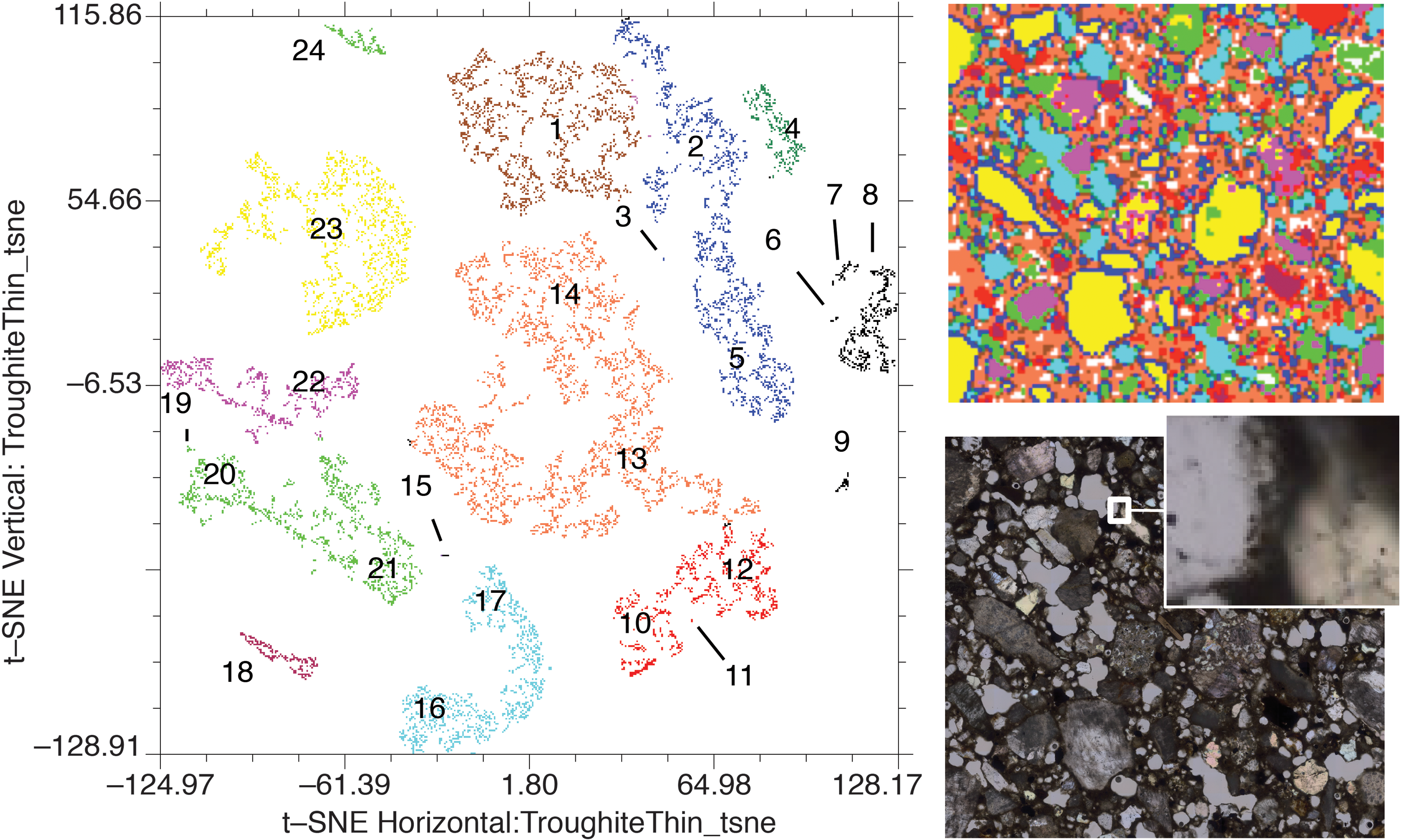
Semi-automated clustering of the Troughite specimen using t-SNE. The projection visualizes the spectral cube as a 2-D map with one point per spectrum. Similar spectra lie close together on the 2-D plane. Axis units are arbitrary. The scatterplot was created automatically, after which colors and numbers were added by hand to emphasize salient groups. Compositional units are (1) calcite cement; (2) edges of feldspar grains; (3) titanium-rich minerals and cement; (4–8) edges of carbonate grains; (9) quartz with diffraction peaks, (10–12) iron oxides; (13–14) iron-rich cement and edges; (15–17) epoxy in voids and along the edges of embedded grains; (18) centers of iron-oxide grains; (19–23) feldspars; (24) edges of calcite crystals. The rightmost panes show the Troughite sample, with the entire field of view spanning 11 mm. Top right: Colors correspond to the classifications in the point cloud. Lower right: Thin section high-resolution microscopic image, co-registered with the PIXL raster. The inset image shows the fine-scale structure of individual grains. (Color graphics available at www.liebertonline.com/ast)

We annotate salient groups with numbers indicating different compositional units that appear as contiguous regions on the sample, and interpret the units based on both thin-scale microscopy and analysis of the spectra. The principal units are (1) calcite cement; (2) edges of feldspar grains; (3) titanium-rich minerals and cement; (4–8) edges of carbonate grains; (9) quartz with diffraction peaks; (10–12) iron oxides; (13–14) iron-rich cement and edges; (15–17) epoxy in voids and along the edges of embedded grains; (18) centers of iron-oxide grains; (19–23) feldspars; (24) edges of calcite crystals. We find that edges of grains are often classified differently than the grains themselves. This is typically related to real differences in the spectra, which can be caused by differences in bulk composition at locations where the X-ray beam excites more than one compositional element (e.g., two separate grains of different mineralogies), by uncorrected differences in the propagation path of X-rays, or by the “footprints” of the detector and emitter. We also find that spectra contaminated by instrument-related effects such as diffraction peaks appear as separate groups. This makes them easy to identify in the t-SNE projections.

4.4. Discussion

Quantitatively and qualitatively, the projection methods produced widely different visual maps. Figure 8 demonstrates that the specific algorithm has an even greater impact than its categorization as linear or nonlinear. Measured by the original performance metric, many of these projections were equally “good” at separating petrological classifications. However, the nonlinear t-SNE is the clear winner in terms of both interpretability (as judged by the k-nn classification) and fidelity (as judged by the ARM scores). It is the top performer for nearly all datasets and metrics. The Shionoha ARM analysis is the only exception, where PCA leads but t-SNE still performs well. t-SNE preserves the fine microstructure evident in maps such as Fig. 10, where nearly all the clusters and local groupings correspond to unique physical features of the sample. The only disadvantage is that filling the entire 2-D plane with meaningful clusters tends to deemphasize the extremes of the most dramatic numerical outliers. Consequently, linear approaches such as classical PCA may still be useful for identifying small endmember points and regions.

The ability to use either t-SNE or PCA representations, and to translate fluidly between region selection on the physical image or in the point cloud, could provide dramatic benefits for early interpretation and exploration of planetary instrument data such as the samples in this work. Planetary instrument operations demand rapid tactical analysis to keep pace with daily operations. Dimensionality reduction can be a valuable first step as a precursor to follow up measurements and quantitative analysis. The same techniques will be more broadly applicable to the next generation of planetary missions that require more aggressive revisions in response to science targets of opportunity. For fast-moving missions such as a Trojan Tour and Rendezvous or Comet Encounter, it will be critical to ingest new data quickly and adapt each new instrument command cycle in response to the latest knowledge of the target. But even as the need for rapid interpretation increases, so does the volume of collected science data. This threatens to become a significant bottleneck in mission science yield. Here, we demonstrate that data-driven visualization can be a useful, general tool to assist these issues. Visual maps of this kind can provide significant improvements for viewing a range of data products. They also promise better quality assurance by quickly highlighting artifacts for reacquisition during instrument operations. It can also enable fast summaries for tactical decisions, revealing trends and patterns. It will provide single-click access to the full catalogue of data and ultimately facilitate scientific discovery.

Samples prepared by polishing in a commercial laboratory are different than the surfaces encountered in situ by a Mars rover. The 2020 rover may include surface preparation systems, such as an abrasion tool, that could remove the surface layer down to depths of approximately 5 mm. This would remove most surface topography and weathering rinds, but the exposed surface would still be rougher than the samples in this study. Moreover, it is possible that dust could collect in the abraded area during preparation, and un-abraded surfaces may still be investigated. These imperfections could create additional spectral diversity that is not scientifically relevant, manifesting as spurious long integrations during adaptive sampling or as extra lobes or groups during visualization. We think it is likely that most surface imperfections would mute, rather than enhance, diversity in the intensities of known line positions. Nonetheless, analyzing samples that are more representative of mission scenarios is a high priority for future study and will proceed as rover sample preparation methods mature.

5. Conclusion

This work has demonstrated principles to expedite astrobiology-relevant science by adding automation at two stages in the data analysis pipeline. We focused on PIXL, which exemplifies a future generation of rastering spectrometer instruments. We presented algorithms for adaptive sampling at millisecond timescales to increase integration time over areas of interest. Simulations on diverse samples showed significant improvements in sample diversity, quantified by the information content of downlinked data for a fixed time budget. Many localized features of interest exhibited unique features that could serve as a cue for spectral servoing. This approach would be most effective for spatially localized features with uniquely distinctive compositions—fortunately, the most likely use case for the technique. A mission-relevant example is the relocation of a detrital grain observed in a stromatolite, or a zircon grain in a sandstone that may yield a U-Pb radiometric date if incorporated into a returned sample.

A second set of experiments dealt with longer timescales, evaluating dimensionality reduction to analyze downlinked data before a fully calibrated and quantitative product became available. We presented a series of experiments applying standard dimensionality reduction strategies to the problem of tactical ground data analysis. While performance varied widely, two methods stand out as particularly useful. Classical PCA provided robust, stable solutions over all datasets in the study and could be useful for identifying outlier compositions during tactical operations. t-SNE was effective at finding structure within the dataset and separating dissimilar datapoints as a precursor to cluster analysis. These techniques could allow for the rapid identification of poor-quality data in large datasets and the semi-automated exclusion of these datapoints in analyses designed to inform rapid tactical decision making during planetary missions. Similarly, these techniques quickly highlight unexpected compositions and subtle compositional gradients that may otherwise not be apparent prior to time-consuming manual data processing.

The principles described in this work apply beyond a Mars 2020 mission; they could assist any mission operating under restricted time resources such as in situ missions to Venus, primitive bodies, the outer planets, or terrestrial field campaigns. The specific algorithms could also apply to other rastering spectrometers capable of collecting large data volumes, including reflectance or fluorescence spectrometers operating in infrared, visible, or ultraviolet wavelengths.

Footnotes

Acknowledgments

This research was performed at the Jet Propulsion Laboratory, California Institute of Technology. It was supported by a technology development grant from AMMOS, the Advanced Multimission Operations System of the National Aeronautics and Space Administration. We acknowledge the invaluable counsel of the PIXL instrument and science teams. We thank Tomoyo Okomura for providing the Shionoha sample.

Author Disclosure Statement

No competing financial interests exist.

Abbreviations Used

References

Akkucuk

(2004) Nonlinear mapping: approaches based on optimizing an index of continuity and applying classical metric MDS on revised distances. PhD dissertation, Rutgers University, New Brunswick, NJ.

Allwood

, Hurowitz

, Elam

W.T.

, and Thompson

D.R.

(2015) High resolution, texture-specific rock chemistry measurement with PIXL micro-XRF [number 2.0707]. In 2015 IEEE Aerospace Conference, IEEE, Piscataway, NJ.

Bartholomew

D.J.

(1987) Latent Variable Models and Factor Analysis, Oxford University Press, New York.

Bearden

J.A.

(1967) X-ray wavelengths. Rev Mod Phys, 39, doi:10.1103/RevModPhys.39.78.

Beegle

L.W.

, Bhartia

, DeFlores

, Darrach

, Kidd

R.D.

, Abbey

, Asher

, Burton

, Clegg

, Conrad

P.G.

, Edgett

, Ehlmann

, Langenhorst

, Fries

, Hug

, Nealson

, Popp

, Sobron

, Steele

, Weins

, and Williford

(2014) SHERLOC: Scanning Habitable Environments with Raman and Luminescence for Organics and Chemicals, an investigation for 2020 [abstract 2835]. In 45th Lunar and Planetary Science Conference Abstracts, LPI contribution 1783, Lunar and Planetary Institute, Houston.

Belkin

and Niyogi

(2003) Laplacian eigenmaps for dimensionality reduction and data representation. Neural Comput, 15:1373–1396.

Bishop

C.M.

(2006) Pattern Recognition and Machine Learning, Springer, New York, NY.

Boardman

J.W.

and Kruse

F.A.

(2011) Analysis of imaging spectrometer data using dimensional geometry and a mixture-tuned matched filtering approach. IEEE Trans Geosci Remote Sens, 49:4138–4152.

Cover

T.M.

and Thomas

J.A.

(2012) Elements of Information Theory, John Wiley & Sons, Hoboken, NJ.

10.

Gorban

A.N.

and Zinovyev

(2010) Principal manifolds and graphs in practice: from molecular biology to dynamical systems. Int J Neural Syst, 20:219–232.

11.

Hinton

G.E.

and Roweis

S.T.

(2002) Stochastic neighbor embedding. In Advances in Neural Information Processing Systems 15, Neural Information Processing Systems (NIPS), Vancouver, Canada, pp 833–840.

12.

Jenkins

(1995) Quantitative X-ray Spectrometry, 2 ^nd ed., CRC Press, Boca Raton, FL.

13.

Lawrence

A.A.N.G.

, Wade

, Hodyss

, and Kozaczek

(2012) A novel micro-xrf for in situ geological exploration of other planets [F-58]. In Denver X-ray Conference, 61st Annual Conference on Applications of X-ray Analysis, Denver, CO.

14.

NASA Science Definition Team. (2014) Report by the NASA Science Definition Team for a 2020 Mars Science Rover, Jet Propulsion Laboratory, California Institute of Technology, Pasadena, CA. Available online at http://mars.jpl.nasa.gov/mars2020/mission/science/objectives

15.

Press

W.H.

, Teukolsky

S.A.

, Vetterling

W.T.

, and Flannery

B.P.

(2007) Numerical Recipes: The Art of Scientific Computing, 3 ^rd ed., Cambridge University Press, New York.

16.

Roweis

S.T.

and Saul

L.K.

(2000) Nonlinear dimensionality reduction by locally linear embedding. Science, 290:2323–2326.

17.

Ryan

, Clayton

, Griffin

, Sie

, and Cousens

(1988) Snip, a statistics-sensitive background treatment for the quantitative analysis of pixel spectra in geoscience applications. Nucl Instrum Methods Phys Res B, 34:396–402.

18.

Schölkopf

, Smola

, and Müller

K.-R.

(1997) Kernel principal component analysis. In Lecture Notes in Computer Science, Vol. 1327, Springer-Verlag, Berlin, pp 583–588.

19.

Shlens

(2005) A tutorial on principal component analysis. Systems Neurobiology Laboratory, Salk Institute for Biological Studies.

20.

Shlens

(2014) Notes on Kullback-Leibler divergence and likelihood. arXiv:1404.2000.

21.

Thompson

D.R.

, Cabrol

N.A.

, Furlong

, Hardgrove

, Low

B.K.H.

, Moersch

, and Wettergreen

(2013) Adaptive sensing of time series with application to remote exploration. In 2013 IEEE International Conference on Robotics and Automation (ICRA), IEEE, Piscataway, NJ, pp 3463–3468.

22.

Thompson

D.R.

, Allwood

, Assad

, Flannery

, Hodyss

, Knowles

, and Wade

(2014) Adaptive sampling for rover X-ray lithochemistry. In 12th International Symposium on Artificial Intelligence, Robotics and Automation in Space (i-SAIRAS), hosted by the Canadian Space Agency, Montréal, Canada.

23.

Tipping

M.E.

and Bishop

C.M.

(1999) Probabilistic principal component analysis. J R Stat Soc Series B Stat Methodol, 61:611–622.

24.

Van der Maaten

and Hinton

(2008) Visualizing data using t-SNE. J Mach Learn Res, 9:2579–2605.

25.

Van der Maaten

L.J.

, Postma

E.O.

, and van den Herik

H.J.

(2009) Dimensionality reduction: a comparative review. J Mach Learn Res, 10:66–71.

26.

Van Grieken

and Markowicz

. (2001) Handbook of X-ray Spectrometry, CRC Press, Boca Raton, FL.

27.

Vogt

, Maser

, and Jacobsen

(2003) Data analysis for X-ray fluorescence imaging. Journal de Physique IV (EDP Sciences Proceedings), 104:617–622.