The Emergence of Life as a First-Order Phase Transition

2.1. Model description

We model the emergence and dynamics of replicators in an artificial prebiotic “chemistry” that consists of two monomer types denoted by “0” and “1.” The properties of our model chemistry are fully specified by the rate constants k _p, k _d, and k _r for polymerization, degradation, and replication, respectively, the finite constant abundances of the two monomeric components 0 and 1, a constant r specifying the minimal length of replicating sequences, and fitness landscapes associated with sequence-specific replication and stability introduced below.

Polymerization occurs via addition of monomers to the end of growing sequences. Polymers can degrade into shorter sequences, which can occur at any bond within a given sequence with equal probability. To simplify the computational model, we adopted a common approximation in models for prebiotic polymerization that the inverse process of two short, but non-monomeric, sequences ligating to produce a longer polymer is sufficiently rare to be neglected (which would be the case, for example, if monomers are much more common than dimers) (Nowak and Ohtsuki, 2008; Manapat et al., 2009; Walker et al., 2012). All sequences of length L ≥ r can self-replicate such that polymers must be sufficiently “complex” to copy themselves (von Kiedrowski, 1986, 1993; Paul and Joyce, 2004). In this study, we set r = 7, such that the appearance of the first replicators is rare but not so rare that we never observe it (Wu and Higgs, 2009). Changing r changes the relative timescale of the transition but does not qualitatively effect the results presented herein.

Since we are interested in the dynamics of replication in this work, and specifically the origins of life, we do not include the effects of mutation, which is well known to play an important role in evolution once life has already emerged (Eigen, 2000) but is not expected to alter the qualitative features of the transition in the simplified model reported here. Therefore, in our model, replication only functions to copy extant sequences and does not produce novelty. Polymerization, however, does produce new sequences, and in our model, novelty is solely introduced through the prebiotic recycling of monomers via degradation and polymerization.

Simulations were implemented using a kinetic Monte Carlo algorithm (Gillespie, 1976, 1977). For more detailed discussion of the implementation of that algorithm in prebiotic recycling chemistries, we refer the reader to the works of Walker et al. (2012) or Vaidya et al. (2013). In what follows, the polymerization, degradation, and replication rate constants were set to k _p = 0.0005, k _d = 0.5000, and k _r = 0.0050, respectively, and the system was initialized with 500 monomers each of 0 and 1 with no polymers present, unless otherwise noted. Since the reaction network is a closed mass system, the initial conditions specify the bulk composition of the system for all time.

2.2. Two fitness landscapes: static and dynamic

To explicitly couple the properties of replicators to those of their environment, we model the fitness of replicators as determined by two factors:

• A static fitness associated with a trade-off between stability and replicative efficiency that is an intrinsic “chemical” property of individual polymer sequences.

The former concept of static fitness encompasses the components of the fitness landscape associated with the properties of specific polymer sequences, without taking any account of the availability of resources. We choose to model selection for replication and stability as a trade-off since in many real-world chemical systems molecules that fold well are typically not good self-replicators, and conversely good self-replicators often do not fold well and are thus less resistant to degradation (Szabó et al., 2002). The latter concept of dynamic, environmentally dictated fitness accounts for the availability of resources (free monomers) in the system and is a unique feature of the resource-dependent replication model presented here (see also Walker et al., 2012, or Vaidya et al., 2013).

Static Fitness. An important question in any model for the emergence of life is how sensitive the observed dynamics are to model parameters or to the fitness landscape imposed in the absence of empirical data. In what follows, we therefore consider several static fitness landscapes, which vary in how well the composition of the “fittest” sequence (or sequences) matches the resource availability in the bulk environment. This allows us to determine whether it is selection on replicators generally or features specific to a particular fitness landscape (and its relationship to abiotic resource distributions) that drive the dynamics observed. We consider four cases:

• Landscape I ( \documentclass{aastex}\usepackage{amsbsy}\usepackage{amsfonts}\usepackage{amssymb}\usepackage{bm}\usepackage{mathrsfs}\usepackage{pifont}\usepackage{stmaryrd}\usepackage{textcomp}\usepackage{portland, xspace}\usepackage{amsmath, amsxtra}\usepackage{upgreek}\pagestyle{empty}\DeclareMathSizes{10}{9}{7}{6}\begin{document}$${\cal L}$$ \end{document} I): Replicators and stable sequences are rare. For the first example, replicative efficiency increases with the number of 0 monomers in a sequence, and stability with the number of 1 monomers, such that homogeneous all-0 sequences with L ≥ 7 are the best replicators, and all-1 sequences are the most stable. Since the bulk composition of the prebiotic environment consists of an equal number of 0 and 1 monomers in our simulations, and polymerization does not favor any specific bond type, good replicators and stable sequences are very rarely produced abiotically, and their composition does not reflect the abiotic distribution of resources.

For \documentclass{aastex}\usepackage{amsbsy}\usepackage{amsfonts}\usepackage{amssymb}\usepackage{bm}\usepackage{mathrsfs}\usepackage{pifont}\usepackage{stmaryrd}\usepackage{textcomp}\usepackage{portland, xspace}\usepackage{amsmath, amsxtra}\usepackage{upgreek}\pagestyle{empty}\DeclareMathSizes{10}{9}{7}{6}\begin{document}$${\cal L}$$ \end{document} I– \documentclass{aastex}\usepackage{amsbsy}\usepackage{amsfonts}\usepackage{amssymb}\usepackage{bm}\usepackage{mathrsfs}\usepackage{pifont}\usepackage{stmaryrd}\usepackage{textcomp}\usepackage{portland, xspace}\usepackage{amsmath, amsxtra}\usepackage{upgreek}\pagestyle{empty}\DeclareMathSizes{10}{9}{7}{6}\begin{document}$${\cal L}$$ \end{document} III, the mathematical form for the trade-off between replication and stability is quantified as \documentclass{aastex}\usepackage{amsbsy}\usepackage{amsfonts}\usepackage{amssymb}\usepackage{bm}\usepackage{mathrsfs}\usepackage{pifont}\usepackage{stmaryrd}\usepackage{textcomp}\usepackage{portland, xspace}\usepackage{amsmath, amsxtra}\usepackage{upgreek}\pagestyle{empty}\DeclareMathSizes{10}{9}{7}{6}\begin{document} \begin{align*} f \left( n \right) = 0.5 + { \frac { { n^2 } } { 2 \left( { 10 + { n^2 } } \right) } } \tag { 1 } \end{align*} \end{document}

following the work of Szabó et al. (2002), who implemented a similar trade-off among attributes of replicating polymers. In our implementation, the replicative fitness of a sequence x_i with length L is quantified by scaling its replication rate k _r by a parameter α _r(x_i ) = 1 + f(n) (which is a number between 1.5 and 2), where n is the quantity that confers replicative efficiency (i.e., 0 monomers, 00 bonds, and 10 bonds in \documentclass{aastex}\usepackage{amsbsy}\usepackage{amsfonts}\usepackage{amssymb}\usepackage{bm}\usepackage{mathrsfs}\usepackage{pifont}\usepackage{stmaryrd}\usepackage{textcomp}\usepackage{portland, xspace}\usepackage{amsmath, amsxtra}\usepackage{upgreek}\pagestyle{empty}\DeclareMathSizes{10}{9}{7}{6}\begin{document}$${\cal L}$$ \end{document} I– \documentclass{aastex}\usepackage{amsbsy}\usepackage{amsfonts}\usepackage{amssymb}\usepackage{bm}\usepackage{mathrsfs}\usepackage{pifont}\usepackage{stmaryrd}\usepackage{textcomp}\usepackage{portland, xspace}\usepackage{amsmath, amsxtra}\usepackage{upgreek}\pagestyle{empty}\DeclareMathSizes{10}{9}{7}{6}\begin{document}$${\cal L}$$ \end{document} III, respectively). Similarly, the stability of sequence x_i is determined by scaling the degradation rate k_d by the parameter α _s(x_i ) = 1 − f(m) (which is a number between 0 and 0.5), where m is the quantity that confers stability (i.e., 1 monomers for \documentclass{aastex}\usepackage{amsbsy}\usepackage{amsfonts}\usepackage{amssymb}\usepackage{bm}\usepackage{mathrsfs}\usepackage{pifont}\usepackage{stmaryrd}\usepackage{textcomp}\usepackage{portland, xspace}\usepackage{amsmath, amsxtra}\usepackage{upgreek}\pagestyle{empty}\DeclareMathSizes{10}{9}{7}{6}\begin{document}$${\cal L}$$ \end{document} I, 01 bonds for \documentclass{aastex}\usepackage{amsbsy}\usepackage{amsfonts}\usepackage{amssymb}\usepackage{bm}\usepackage{mathrsfs}\usepackage{pifont}\usepackage{stmaryrd}\usepackage{textcomp}\usepackage{portland, xspace}\usepackage{amsmath, amsxtra}\usepackage{upgreek}\pagestyle{empty}\DeclareMathSizes{10}{9}{7}{6}\begin{document}$${\cal L}$$ \end{document} II and \documentclass{aastex}\usepackage{amsbsy}\usepackage{amsfonts}\usepackage{amssymb}\usepackage{bm}\usepackage{mathrsfs}\usepackage{pifont}\usepackage{stmaryrd}\usepackage{textcomp}\usepackage{portland, xspace}\usepackage{amsmath, amsxtra}\usepackage{upgreek}\pagestyle{empty}\DeclareMathSizes{10}{9}{7}{6}\begin{document}$${\cal L}$$ \end{document} III). Sequences with L < 7 do not replicate, so only the stability landscape is relevant for short sequences. In each example, this establishes a fitness landscape intrinsic to a polymer's specific sequence that is fixed within a given environmental context.

Dynamic Fitness. Since we are interested in the coupling between replicators and their environment, we also introduce an extrinsic, dynamic term to replicative efficiency, which is determined by the availability of free monomers in the environment. To this end, the replication rate for sequence x_i is weighted by a factor \documentclass{aastex}\usepackage{amsbsy}\usepackage{amsfonts}\usepackage{amssymb}\usepackage{bm}\usepackage{mathrsfs}\usepackage{pifont}\usepackage{stmaryrd}\usepackage{textcomp}\usepackage{portland, xspace}\usepackage{amsmath, amsxtra}\usepackage{upgreek}\pagestyle{empty}\DeclareMathSizes{10}{9}{7}{6}\begin{document}$$\beta \left( {{x_i}} \right) = \sum \nolimits_{{n_i}}^{L - 1} {{y_{{n_i}}}{y_{{n_i} + 1}}}$$ \end{document} where y_n is the abundance of the monomer species at position n in sequence x_i . This term yields a computationally tractable resource-dependent replication rate that is also sequence-dependent. This term may be motivated as a sum over all possible nucleation events on a template [see, e.g., Vaidya et al. (2013) for an explicit example as applies to ribozyme recycling]. As such, the replication rate of a given sequence x_i depends in part on how well its sequence composition matches the relative abundances of 0 and 1 monomers in the environment. Since the abundances of 0 and 1 monomers change over time as monomers are consumed via polymerization and replication and generated via degradation, this creates a dynamic, environmentally dictated fitness landscape that is a central feature of any resource-constrained dynamics. We expect qualitative features of the dynamics observed here to be a general feature of species-specific and resource-dependent replication, independent of the particular functional form of β(x_i ).

2.3. Tracking the selection of replicators with mutual information

To characterize the dynamics of the observed phase transition, we employ mutual information, a common tool in information theory, which measures the mutual dependence of two variables within a dynamic time series by quantifying how much information the two variables share in common. We use mutual information, \documentclass{aastex}\usepackage{amsbsy}\usepackage{amsfonts}\usepackage{amssymb}\usepackage{bm}\usepackage{mathrsfs}\usepackage{pifont}\usepackage{stmaryrd}\usepackage{textcomp}\usepackage{portland, xspace}\usepackage{amsmath, amsxtra}\usepackage{upgreek}\pagestyle{empty}\DeclareMathSizes{10}{9}{7}{6}\begin{document}$${\cal I}$$ \end{document} , to measure the extent to which the composition of replicators is determined by their environment, and vice versa. We define the sets R and E, which contain ordered pairs that track the number of 0 and 1 monomers in replicators (R) and in free monomers in the environment (E), allowing us to measure \documentclass{aastex}\usepackage{amsbsy}\usepackage{amsfonts}\usepackage{amssymb}\usepackage{bm}\usepackage{mathrsfs}\usepackage{pifont}\usepackage{stmaryrd}\usepackage{textcomp}\usepackage{portland, xspace}\usepackage{amsmath, amsxtra}\usepackage{upgreek}\pagestyle{empty}\DeclareMathSizes{10}{9}{7}{6}\begin{document}$${\cal I}$$ \end{document} (R : E), defined as the mutual information shared between replicators and their environment. See the appendix for additional details.

3.1. A first-order phase transition from nonlife to life

Two long-lived states are observed, which we nominally call nonlife and life. These two phases are dominated by polymer formation via polymerization or via replication, respectively. While the nonlife phase here shares features in common with prelife as previously characterized (Nowak and Ohtsuki, 2008), it also has some striking differences—we therefore use nonlife rather than prelife (in our system, many transitions fail to complete, so the emergence of replicators and life is not inevitable; thus nonlife is more appropriate).

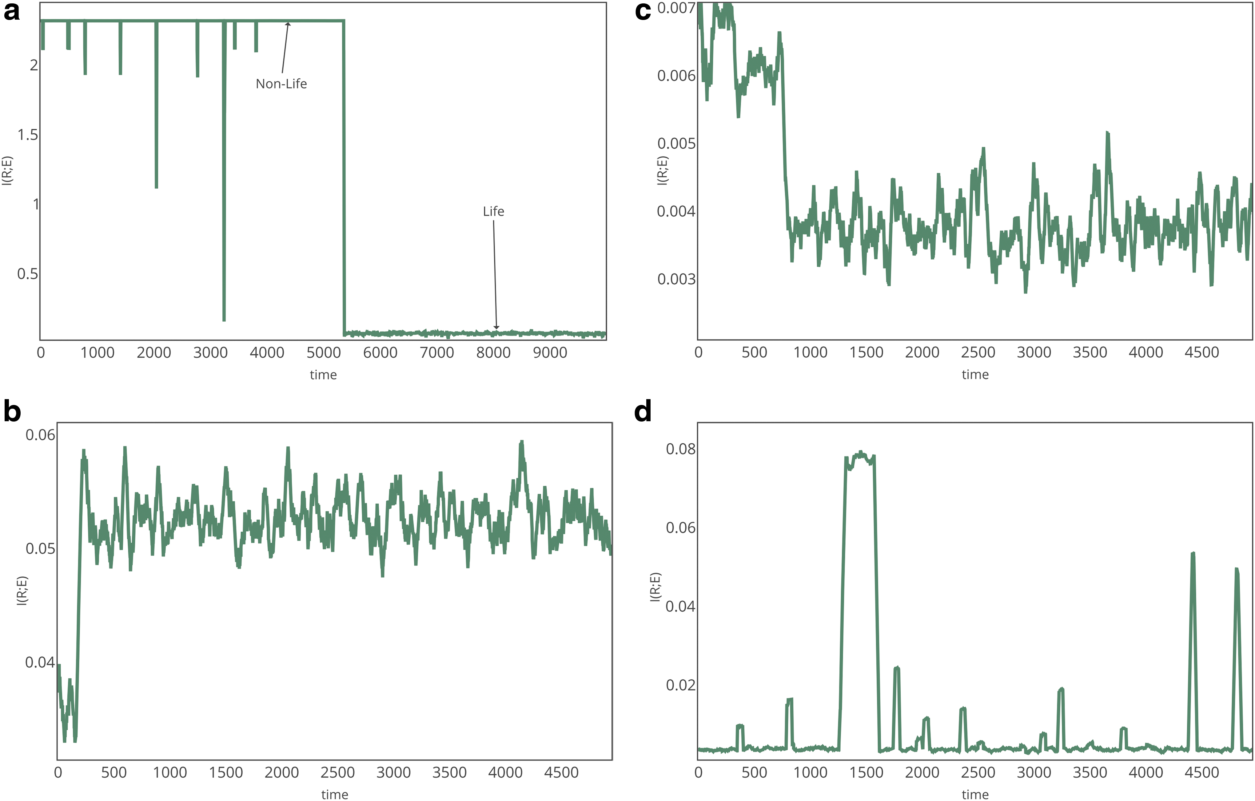
For fixed values of k _p, k _d, and k _r, the system exhibits a spontaneous and abrupt transition from nonlife to life for all four fitness landscapes investigated. The transition is accurately tracked by measuring the mutual information \documentclass{aastex}\usepackage{amsbsy}\usepackage{amsfonts}\usepackage{amssymb}\usepackage{bm}\usepackage{mathrsfs}\usepackage{pifont}\usepackage{stmaryrd}\usepackage{textcomp}\usepackage{portland, xspace}\usepackage{amsmath, amsxtra}\usepackage{upgreek}\pagestyle{empty}\DeclareMathSizes{10}{9}{7}{6}\begin{document}$${\cal I}$$ \end{document} (R;E) between the composition of extant replicators and free monomer resources, as shown in Fig. 1. The details of the transition are dependent on the static fitness landscape chosen, but the transition exists independent of the nature of the landscape chosen. For \documentclass{aastex}\usepackage{amsbsy}\usepackage{amsfonts}\usepackage{amssymb}\usepackage{bm}\usepackage{mathrsfs}\usepackage{pifont}\usepackage{stmaryrd}\usepackage{textcomp}\usepackage{portland, xspace}\usepackage{amsmath, amsxtra}\usepackage{upgreek}\pagestyle{empty}\DeclareMathSizes{10}{9}{7}{6}\begin{document}$${\cal L}$$ \end{document} I (Fig. 1, top left), mutual information decreases through the transition, since the composition of selected replicators differs from that of their environment. This is true also of \documentclass{aastex}\usepackage{amsbsy}\usepackage{amsfonts}\usepackage{amssymb}\usepackage{bm}\usepackage{mathrsfs}\usepackage{pifont}\usepackage{stmaryrd}\usepackage{textcomp}\usepackage{portland, xspace}\usepackage{amsmath, amsxtra}\usepackage{upgreek}\pagestyle{empty}\DeclareMathSizes{10}{9}{7}{6}\begin{document}$${\cal L}$$ \end{document} II (Fig. 1, top right); however, the magnitude of the difference in \documentclass{aastex}\usepackage{amsbsy}\usepackage{amsfonts}\usepackage{amssymb}\usepackage{bm}\usepackage{mathrsfs}\usepackage{pifont}\usepackage{stmaryrd}\usepackage{textcomp}\usepackage{portland, xspace}\usepackage{amsmath, amsxtra}\usepackage{upgreek}\pagestyle{empty}\DeclareMathSizes{10}{9}{7}{6}\begin{document}$${\cal I}$$ \end{document} (R;E) between the two phases is less dramatic due to selection of stable, less efficiently replicating sequences whose composition does match bulk resources, in addition to efficient replicators whose composition does not. For \documentclass{aastex}\usepackage{amsbsy}\usepackage{amsfonts}\usepackage{amssymb}\usepackage{bm}\usepackage{mathrsfs}\usepackage{pifont}\usepackage{stmaryrd}\usepackage{textcomp}\usepackage{portland, xspace}\usepackage{amsmath, amsxtra}\usepackage{upgreek}\pagestyle{empty}\DeclareMathSizes{10}{9}{7}{6}\begin{document}$${\cal L}$$ \end{document} III (Fig. 1, bottom left), mutual information increases since the composition of selected replicators reflects the bulk composition of their environment. For \documentclass{aastex}\usepackage{amsbsy}\usepackage{amsfonts}\usepackage{amssymb}\usepackage{bm}\usepackage{mathrsfs}\usepackage{pifont}\usepackage{stmaryrd}\usepackage{textcomp}\usepackage{portland, xspace}\usepackage{amsmath, amsxtra}\usepackage{upgreek}\pagestyle{empty}\DeclareMathSizes{10}{9}{7}{6}\begin{document}$${\cal L}$$ \end{document} IV (Fig. 1, bottom right), where there is no selection on specific sequences, the transition is visible in the rapid changes in the mutual information between a state of high and a state of low mutual information, as stochastically determined replicators are selected and accumulate through exponential growth, until a large fluctuation leads to a different replicator that dominates. For \documentclass{aastex}\usepackage{amsbsy}\usepackage{amsfonts}\usepackage{amssymb}\usepackage{bm}\usepackage{mathrsfs}\usepackage{pifont}\usepackage{stmaryrd}\usepackage{textcomp}\usepackage{portland, xspace}\usepackage{amsmath, amsxtra}\usepackage{upgreek}\pagestyle{empty}\DeclareMathSizes{10}{9}{7}{6}\begin{document}$${\cal L}$$ \end{document} IV, the transition is frustrated for the particular choice of parameters: sequences are transiently selected, but the system settles back before the sequences dominate. The absolute value of \documentclass{aastex}\usepackage{amsbsy}\usepackage{amsfonts}\usepackage{amssymb}\usepackage{bm}\usepackage{mathrsfs}\usepackage{pifont}\usepackage{stmaryrd}\usepackage{textcomp}\usepackage{portland, xspace}\usepackage{amsmath, amsxtra}\usepackage{upgreek}\pagestyle{empty}\DeclareMathSizes{10}{9}{7}{6}\begin{document}$${\cal I}$$ \end{document} (R;E) and the size of the fluctuations are sensitive to the fitness landscape imposed; however, the presence of an abrupt, spontaneous transition is apparent in each case and accurately tracks the onset of selection on the properties of replicators.

OPEN IN VIEWER

FIG. 1.

Typical time series of the mutual information shared between replicators and their environment (free monomers) for each fitness landscape. Top left: \documentclass{aastex}\usepackage{amsbsy}\usepackage{amsfonts}\usepackage{amssymb}\usepackage{bm}\usepackage{mathrsfs}\usepackage{pifont}\usepackage{stmaryrd}\usepackage{textcomp}\usepackage{portland, xspace}\usepackage{amsmath, amsxtra}\usepackage{upgreek}\pagestyle{empty}\DeclareMathSizes{10}{9}{7}{6}\begin{document}$${\cal L}$$ \end{document} I. Top right: \documentclass{aastex}\usepackage{amsbsy}\usepackage{amsfonts}\usepackage{amssymb}\usepackage{bm}\usepackage{mathrsfs}\usepackage{pifont}\usepackage{stmaryrd}\usepackage{textcomp}\usepackage{portland, xspace}\usepackage{amsmath, amsxtra}\usepackage{upgreek}\pagestyle{empty}\DeclareMathSizes{10}{9}{7}{6}\begin{document}$${\cal L}$$ \end{document} II. Bottom left: \documentclass{aastex}\usepackage{amsbsy}\usepackage{amsfonts}\usepackage{amssymb}\usepackage{bm}\usepackage{mathrsfs}\usepackage{pifont}\usepackage{stmaryrd}\usepackage{textcomp}\usepackage{portland, xspace}\usepackage{amsmath, amsxtra}\usepackage{upgreek}\pagestyle{empty}\DeclareMathSizes{10}{9}{7}{6}\begin{document}$${\cal L}$$ \end{document} III. Bottom right: \documentclass{aastex}\usepackage{amsbsy}\usepackage{amsfonts}\usepackage{amssymb}\usepackage{bm}\usepackage{mathrsfs}\usepackage{pifont}\usepackage{stmaryrd}\usepackage{textcomp}\usepackage{portland, xspace}\usepackage{amsmath, amsxtra}\usepackage{upgreek}\pagestyle{empty}\DeclareMathSizes{10}{9}{7}{6}\begin{document}$${\cal L}$$ \end{document} IV. The phase transition is clearly evident in the abrupt shift (or shifts) in \documentclass{aastex}\usepackage{amsbsy}\usepackage{amsfonts}\usepackage{amssymb}\usepackage{bm}\usepackage{mathrsfs}\usepackage{pifont}\usepackage{stmaryrd}\usepackage{textcomp}\usepackage{portland, xspace}\usepackage{amsmath, amsxtra}\usepackage{upgreek}\pagestyle{empty}\DeclareMathSizes{10}{9}{7}{6}\begin{document}$${\cal I}$$ \end{document} (R;E) observable in each case.

Since the transition is apparent for each landscape explored, we focus on \documentclass{aastex}\usepackage{amsbsy}\usepackage{amsfonts}\usepackage{amssymb}\usepackage{bm}\usepackage{mathrsfs}\usepackage{pifont}\usepackage{stmaryrd}\usepackage{textcomp}\usepackage{portland, xspace}\usepackage{amsmath, amsxtra}\usepackage{upgreek}\pagestyle{empty}\DeclareMathSizes{10}{9}{7}{6}\begin{document}$${\cal L}$$ \end{document} I, as we expect this landscape to exhibit the most interesting dynamics, given that replicators and stable sequences are rare and not readily produced prebiotically. We also expect this case to be the most realistic, as functional biopolymers are sparse in sequence space and often do not share their composition with the ambient environment.

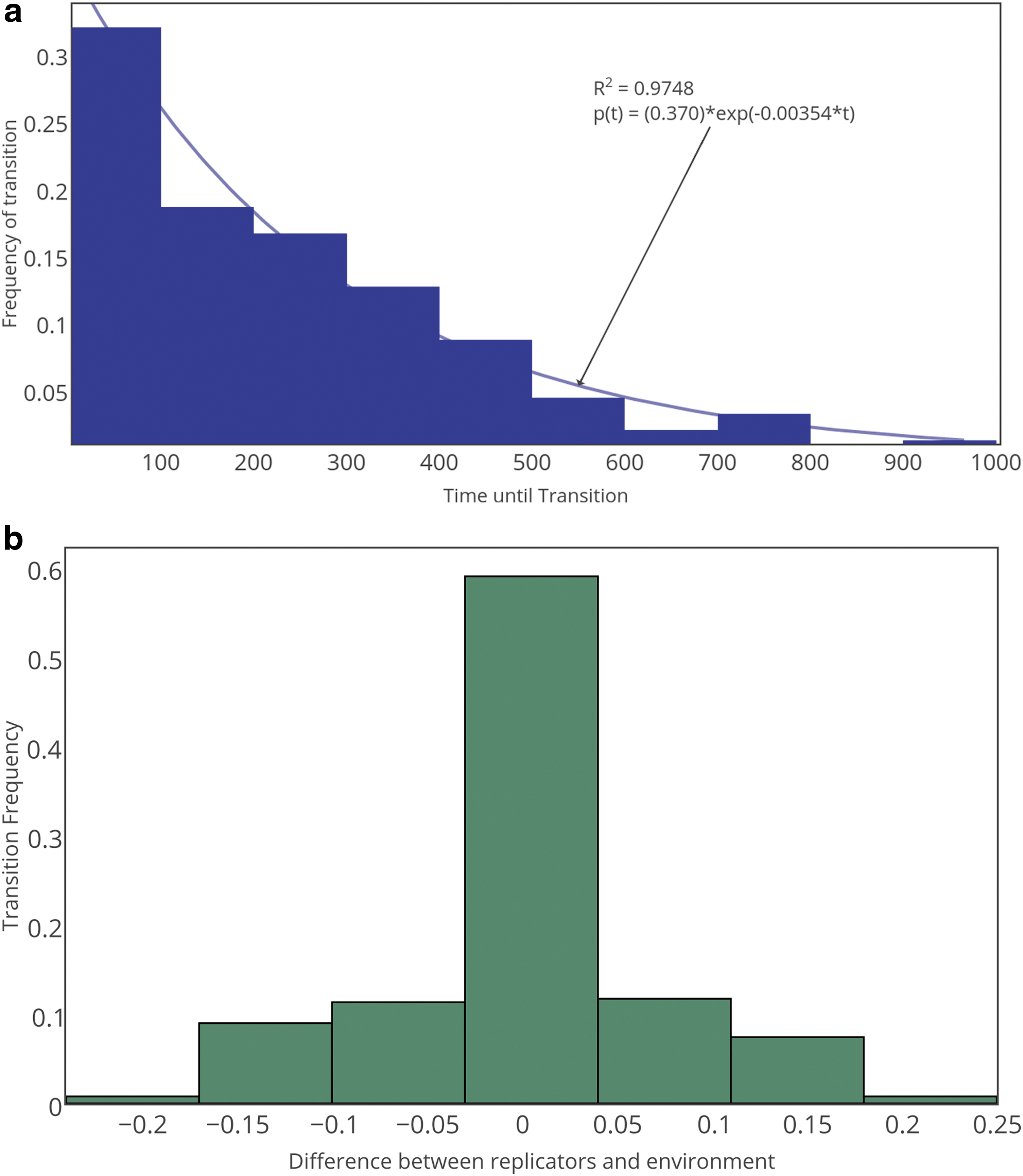
The dynamics of the transition from nonlife to life displays many hallmarks of physical first-order phase transitions. The results of a Kolmogorov–Smirnov (KS) test suggest that the distribution of wait times until the transition successfully completes is consistent with the expected exponential distribution (Fig. 2, panel a) (Smith and Morowitz, 2016). The frequency that the transition occurs is dependent on both the composition of replicators and the environment (Fig. 2, panel b). This is distinct from other models that do not account for environmental feedback (Nowak and Ohtsuki, 2008; Wu and Higgs, 2009)—here, the transition is not coincident with the first “discovery” of a sequence capable of replication, since replicators can exist in nonlife. Instead, the transition occurs when replicators and the environment share similar resource distributions (high extrinsic fitness). Since both monomer species are equally abundant in the initial distribution of resources for the examples reported here, the nucleation event is typically mediated by a heterogeneous replicator (or replicators) composed of a roughly equal number of 0s and 1s (this is true for all four landscapes). These are not the sequences that are ultimately selected in the life phase for \documentclass{aastex}\usepackage{amsbsy}\usepackage{amsfonts}\usepackage{amssymb}\usepackage{bm}\usepackage{mathrsfs}\usepackage{pifont}\usepackage{stmaryrd}\usepackage{textcomp}\usepackage{portland, xspace}\usepackage{amsmath, amsxtra}\usepackage{upgreek}\pagestyle{empty}\DeclareMathSizes{10}{9}{7}{6}\begin{document}$${\cal L}$$ \end{document} I, which include only the homogeneous, fit sequences. Given that the transition is spontaneous, abrupt, and exponentially distributed, we consider the dynamics to be indicative of a genuine first-order phase transition. We note that, similar to other first-order transitions, there are often many frustrated transitions prior to a successful phase transition (see Fig. 1, top left), which can occur when lack of selection on fit sequences leads to a failure in the transition to run to completion (see also Fig. 1, bottom right).

OPEN IN VIEWER

FIG. 2.

Panel a: The distribution of waiting times until the phase transition occurs for \documentclass{aastex}\usepackage{amsbsy}\usepackage{amsfonts}\usepackage{amssymb}\usepackage{bm}\usepackage{mathrsfs}\usepackage{pifont}\usepackage{stmaryrd}\usepackage{textcomp}\usepackage{portland, xspace}\usepackage{amsmath, amsxtra}\usepackage{upgreek}\pagestyle{empty}\DeclareMathSizes{10}{9}{7}{6}\begin{document}$${\cal L}$$ \end{document} I is shown. It follows an exponential distribution, indicative of a first-order phase transition due to large fluctuations. Panel b: The frequency of successful phase transitions for \documentclass{aastex}\usepackage{amsbsy}\usepackage{amsfonts}\usepackage{amssymb}\usepackage{bm}\usepackage{mathrsfs}\usepackage{pifont}\usepackage{stmaryrd}\usepackage{textcomp}\usepackage{portland, xspace}\usepackage{amsmath, amsxtra}\usepackage{upgreek}\pagestyle{empty}\DeclareMathSizes{10}{9}{7}{6}\begin{document}$${\cal L}$$ \end{document} I as a function of the difference between the composition of extant replicators and their environment. Data shown is for an ensemble statistic of 256 simulations. Simulation parameters were set as k _p = 0.0005, k _d = 0.5000, and k _r = 0.0050 for both figures.

3.2. The dynamics of the transition from nonlife to life

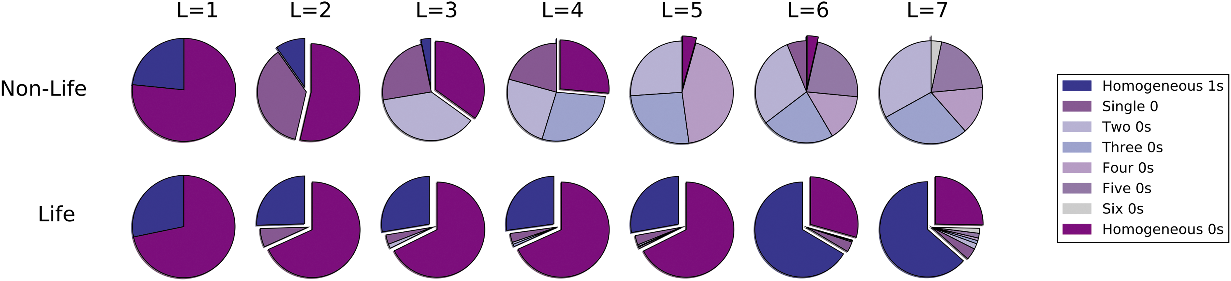
In the nonlife phase, long sequences are exponentially rare, and the majority of system mass is in monomers and dimers (not shown). Sequences of all lengths have relatively similar composition, as shown in the top panel of Fig. 3. The composition of extant polymers is reflective of the combined effects of the abiotic availability of resources and, for \documentclass{aastex}\usepackage{amsbsy}\usepackage{amsfonts}\usepackage{amssymb}\usepackage{bm}\usepackage{mathrsfs}\usepackage{pifont}\usepackage{stmaryrd}\usepackage{textcomp}\usepackage{portland, xspace}\usepackage{amsmath, amsxtra}\usepackage{upgreek}\pagestyle{empty}\DeclareMathSizes{10}{9}{7}{6}\begin{document}$${\cal L}$$ \end{document} I– \documentclass{aastex}\usepackage{amsbsy}\usepackage{amsfonts}\usepackage{amssymb}\usepackage{bm}\usepackage{mathrsfs}\usepackage{pifont}\usepackage{stmaryrd}\usepackage{textcomp}\usepackage{portland, xspace}\usepackage{amsmath, amsxtra}\usepackage{upgreek}\pagestyle{empty}\DeclareMathSizes{10}{9}{7}{6}\begin{document}$${\cal L}$$ \end{document} III, the stability landscape established by Eq. 1. Replicators can exist in the nonlife phase, albeit at exponentially low abundance. These typically have compositions reflective of the abiotic distribution of resources and form via polymerization.

OPEN IN VIEWER

FIG. 3.

Ensemble averaged compositions of all sequences with L ≤ 7 for \documentclass{aastex}\usepackage{amsbsy}\usepackage{amsfonts}\usepackage{amssymb}\usepackage{bm}\usepackage{mathrsfs}\usepackage{pifont}\usepackage{stmaryrd}\usepackage{textcomp}\usepackage{portland, xspace}\usepackage{amsmath, amsxtra}\usepackage{upgreek}\pagestyle{empty}\DeclareMathSizes{10}{9}{7}{6}\begin{document}$${\cal L}$$ \end{document} I. The distributions in the top panel characterize the nonlife phase (no selection on replicators) and in the bottom panel characterize the life phase (selection on replicators). Data is averaged over 100 simulations, and simulation parameters are k _p = 0.0005, k _d = 0.5000, and k _r = 0.0050.

In the life phase, the composition of replicators need not reflect the bulk composition of the environment; instead, replicator composition is determined by selection of the fittest sequences. This can in turn lead to restructuring of the distribution of resources in the environment, as shown in Fig. 3 for \documentclass{aastex}\usepackage{amsbsy}\usepackage{amsfonts}\usepackage{amssymb}\usepackage{bm}\usepackage{mathrsfs}\usepackage{pifont}\usepackage{stmaryrd}\usepackage{textcomp}\usepackage{portland, xspace}\usepackage{amsmath, amsxtra}\usepackage{upgreek}\pagestyle{empty}\DeclareMathSizes{10}{9}{7}{6}\begin{document}$${\cal L}$$ \end{document} I, where selected replicators are primarily homogeneous 1s or 0s. Due to resource constraints, selection on replicators drives a transition in the composition of shorter sequences. In the life phase, short sequences obtain the opposite compositional signature to that of replicators (bottom panel, Fig. 3). The compositional reversal is seen only below L = 6. Although L = 6 sequences cannot replicate, they are formed primarily via degradation of L = 7 replicators; thus their formation is dominated by self-replication (via formation, then degradation of L = 7 sequences). In the life phase, replicators are selected based on their intrinsic fitness and not strictly how well their composition matches the environment. The defining feature of the life phase is therefore not necessarily the presence of replicators, which exist in both phases. Instead, the defining characteristic of “life” in this model is that the distribution of resources is dictated by selection on the properties of replicators, and that selection only operates in the life phase.

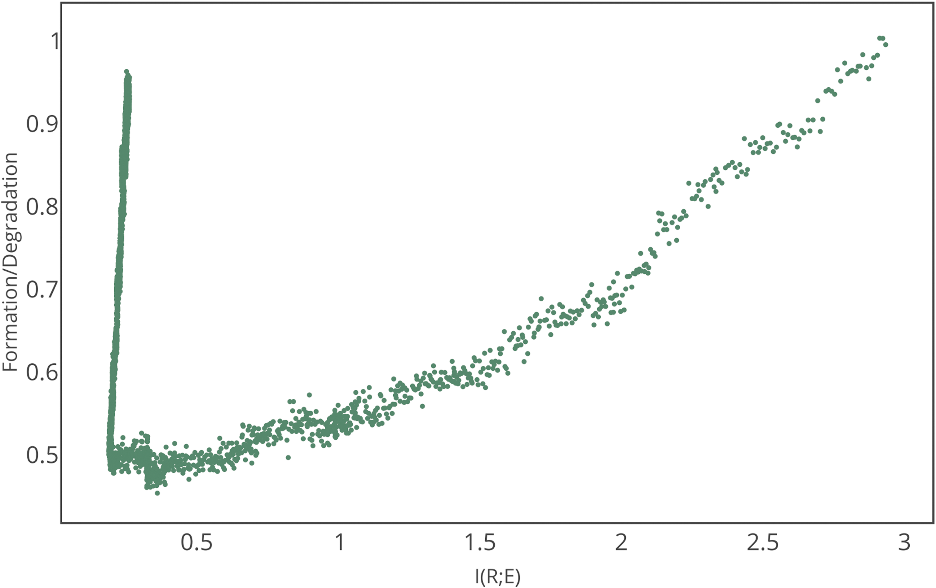
Figure 3 demonstrates that, due to resource constraints, the selection of replicators can coincide with dynamic restructuring of the entire system [including both monomer and nonreplicating (L < 7) sequence populations]. Figure 4 shows an ensemble averaged phase space trajectory through this restructuring for \documentclass{aastex}\usepackage{amsbsy}\usepackage{amsfonts}\usepackage{amssymb}\usepackage{bm}\usepackage{mathrsfs}\usepackage{pifont}\usepackage{stmaryrd}\usepackage{textcomp}\usepackage{portland, xspace}\usepackage{amsmath, amsxtra}\usepackage{upgreek}\pagestyle{empty}\DeclareMathSizes{10}{9}{7}{6}\begin{document}$${\cal L}$$ \end{document} I. The phase transition moving from nonlife to life phases is highly unstable and dominated by degradation. In both the nonlife and life phases, polymer formation rates (polymerization and replication) balance rates for polymer degradation, with ratios of formation/degradation ∼1. However, the life and nonlife phases are clearly distinguished in phase space by very different values for the mutual information [here \documentclass{aastex}\usepackage{amsbsy}\usepackage{amsfonts}\usepackage{amssymb}\usepackage{bm}\usepackage{mathrsfs}\usepackage{pifont}\usepackage{stmaryrd}\usepackage{textcomp}\usepackage{portland, xspace}\usepackage{amsmath, amsxtra}\usepackage{upgreek}\pagestyle{empty}\DeclareMathSizes{10}{9}{7}{6}\begin{document}$${\cal I}$$ \end{document} (R;E) ∼ 3.0 for nonlife and \documentclass{aastex}\usepackage{amsbsy}\usepackage{amsfonts}\usepackage{amssymb}\usepackage{bm}\usepackage{mathrsfs}\usepackage{pifont}\usepackage{stmaryrd}\usepackage{textcomp}\usepackage{portland, xspace}\usepackage{amsmath, amsxtra}\usepackage{upgreek}\pagestyle{empty}\DeclareMathSizes{10}{9}{7}{6}\begin{document}$${\cal I}$$ \end{document} (R;E) ∼ 0.25 for life, for results in Fig. 4].

OPEN IN VIEWER

FIG. 4.

Phase trajectory for an ensemble of 100 systems transitioning from nonlife to life (plotted vs. time, the system would move from left to right). Axes are the mutual information \documentclass{aastex}\usepackage{amsbsy}\usepackage{amsfonts}\usepackage{amssymb}\usepackage{bm}\usepackage{mathrsfs}\usepackage{pifont}\usepackage{stmaryrd}\usepackage{textcomp}\usepackage{portland, xspace}\usepackage{amsmath, amsxtra}\usepackage{upgreek}\pagestyle{empty}\DeclareMathSizes{10}{9}{7}{6}\begin{document}$${\cal I}$$ \end{document} (R;E) between replicators and environment (x axis) and the ratio of formation (polymerization and replication) to degradation rates (y axis). Simulation parameters are k _p = 0.0005, k _d = 0.5000, and k _r = 0.0050.

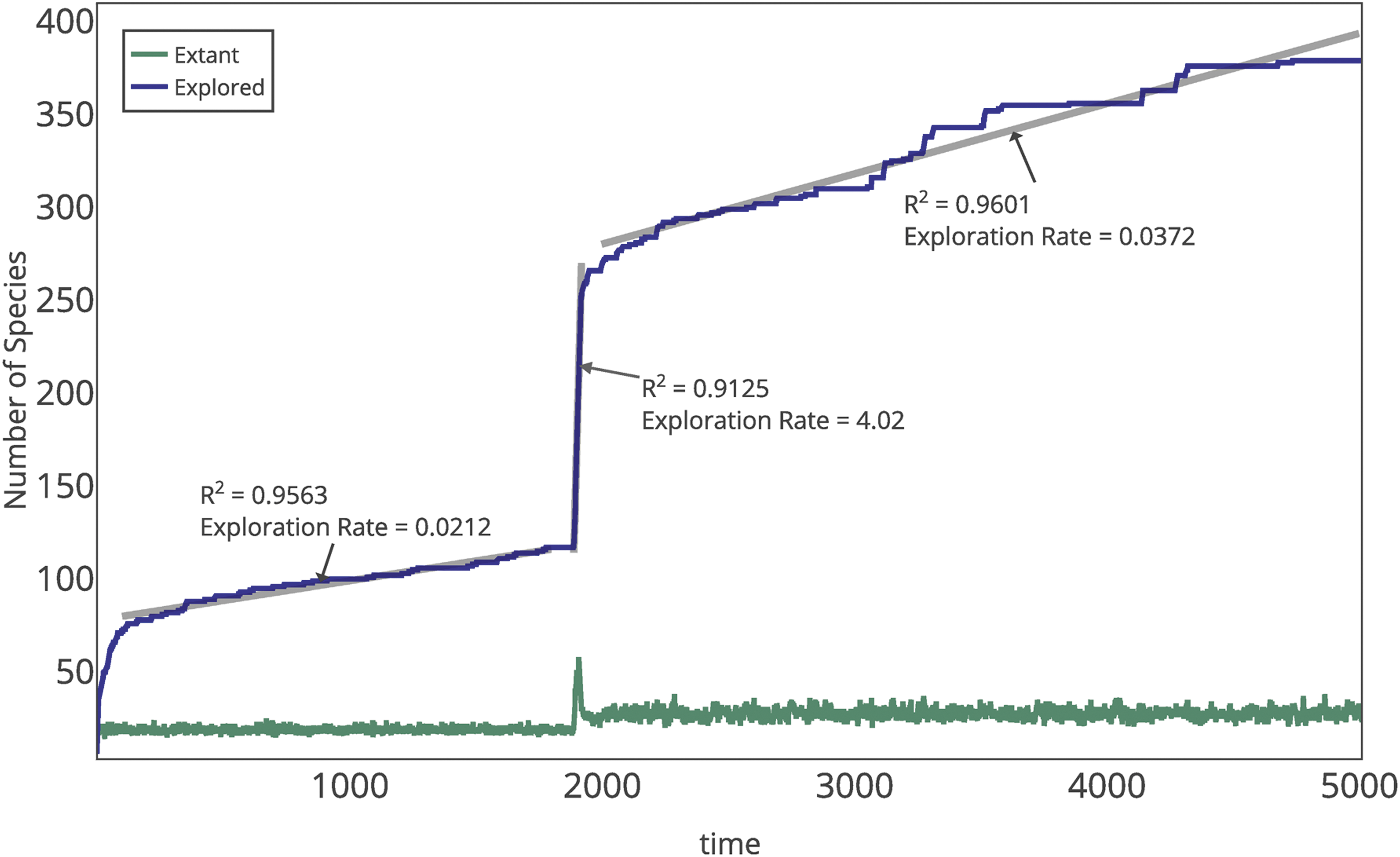
The rampant degradation observed through the phase transition results in a rapid and dramatic restructuring of the extant polymer population and a steep slope in the rate of sequence exploration, as observed in Fig. 5. This is characteristic of the phase transition from nonlife to life, independent of the replicative fitness landscape. This restructuring arises as a result of reallocation of mass from shorter sequences to replicators, which must occur via degradation to monomers that can then be consumed via replication. The extant diversity and the rate of introduction of new sequences are both higher in the life phase than the nonlife phase (Fig. 5), which is attributable to the higher turnover rate of resources in the life phase (due to the higher assembly rate of polymers via replication).

OPEN IN VIEWER

FIG. 5.

Exemplary time series for the extant species population size and total number of sequences explored by the system. Linear fits to the explored species are shown. The exploration rate is 75% faster during the life phase compared to the nonlife phase and is 2 orders of magnitude larger during the transition. Simulation parameters are k _p = 0.0005, k _d = 0.5000, and k _r = 0.0050.

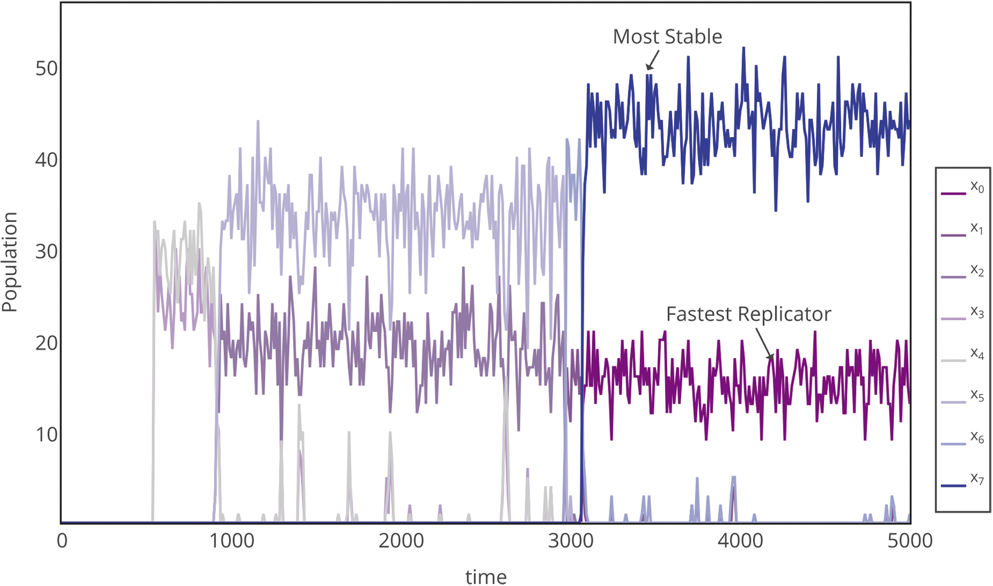
Shown in Fig. 6 is an example time series for the evolution of all sequences with L = 7 for \documentclass{aastex}\usepackage{amsbsy}\usepackage{amsfonts}\usepackage{amssymb}\usepackage{bm}\usepackage{mathrsfs}\usepackage{pifont}\usepackage{stmaryrd}\usepackage{textcomp}\usepackage{portland, xspace}\usepackage{amsmath, amsxtra}\usepackage{upgreek}\pagestyle{empty}\DeclareMathSizes{10}{9}{7}{6}\begin{document}$${\cal L}$$ \end{document} I, binned by sequence composition, for a set of parameters where the transition is prolonged enough to resolve details of the restructuring. Resource constraints enforce selection of sequences in complementary pairs that maintain the symmetry of the bulk resource distribution of the environment (50% 0s and 50% 1s). The system subsequently undergoes a series of abrupt transitions associated with increasing sequence homogeneity, where replicator composition increasingly departs from that of the bulk environment.

OPEN IN VIEWER

FIG. 6.

Series of transitions in the selection of fit, homogeneous “0” and “1” length L = 7 replicators for \documentclass{aastex}\usepackage{amsbsy}\usepackage{amsfonts}\usepackage{amssymb}\usepackage{bm}\usepackage{mathrsfs}\usepackage{pifont}\usepackage{stmaryrd}\usepackage{textcomp}\usepackage{portland, xspace}\usepackage{amsmath, amsxtra}\usepackage{upgreek}\pagestyle{empty}\DeclareMathSizes{10}{9}{7}{6}\begin{document}$${\cal L}$$ \end{document} I. Here, the subscript denotes the number of “1” monomers in the sequence (e.g., x ₀ contains no “1s,” x ₁ bins all polymers with a single “1” monomer, and x ₇ contains all “1s”). Simulation parameters are k _p = 0.0005, k _d = 0.9000, and k _r = 1.000.

3.3. The timescale for life's emergence

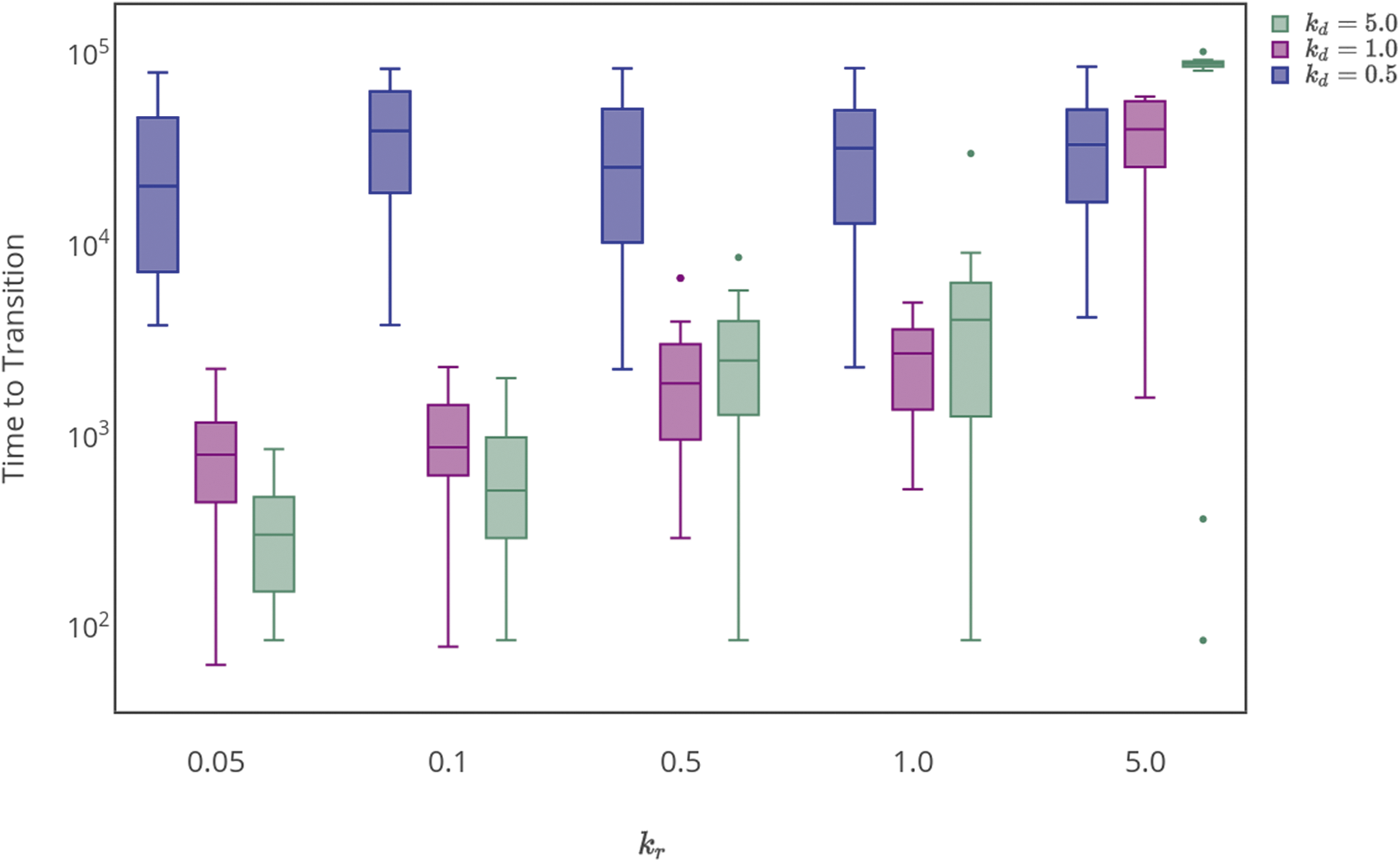
The phase transition from nonlife to life described here is a robust feature of the dynamics, observed for different fitness landscapes with qualitatively similar features. Here, we demonstrate that the observed features are also qualitatively robust over a large range of parameter values. Quantitative differences arise in the final abundances of replicators and in the timescale for the transition to occur, which are both sensitive to the specific details of the prebiotic chemistry under consideration. Figure 7 shows the average time to complete the phase transition as a function of the degradation and replication rate constants, k _d and k _r, for \documentclass{aastex}\usepackage{amsbsy}\usepackage{amsfonts}\usepackage{amssymb}\usepackage{bm}\usepackage{mathrsfs}\usepackage{pifont}\usepackage{stmaryrd}\usepackage{textcomp}\usepackage{portland, xspace}\usepackage{amsmath, amsxtra}\usepackage{upgreek}\pagestyle{empty}\DeclareMathSizes{10}{9}{7}{6}\begin{document}$${\cal L}$$ \end{document} I. For the results presented, the transition was identified as complete when 75% of the total replicating mass was allocated in homogeneous (fit) sequences.

OPEN IN VIEWER

FIG. 7.

Timescale for completing the phase transition as a function of reaction rate constants for replication k _r. Data from 25 simulations is shown; all data points are included in the box and whisker plots. The center line for each distribution is the median, the boxes contain half the data points, and the bars show the range. Three values of the degradation rate constant k _d are shown: 5.0 (blue), 1.0 (purple), 0.5 (green). The polymerization rate constant was fixed at k _p = 0.0005.

One might a priori expect the transition to be most rapid (favored) for fast replication (high k _r) and slow degradation (low k _d); however, this is not always observed. For high degradation rate k _d = 5.0, the time to the transition is largely independent of k _r (Fig. 7). Lowering the degradation rate (k _d = 1.0 and k _d = 0.5, Fig. 7) increases the dependence of the transition time on k _r, which, on average, occurs most rapidly for relatively low k _r. This counterintuitive behavior arises as a result of the resource constraints. For high degradation rates, there is a high rate of turnover that increases the likelihood of discovering functionally fit sequences, but the probability of survival is low, so the transition time is long regardless of replicative efficiency. For lower degradation rates, high replication rates lock resources in less fit sequences, frustrating the system's restructuring and leading to long transition times.

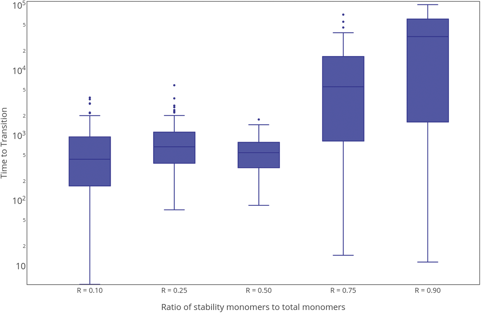
The rate of degradative recycling seems to be the primary factor in determining the transition timescale. Figure 8 shows the transition time observed for different abiotic resource abundances, quantified by the ratio R of the total number of 1 monomers to total system mass. The transition timescale is not expected to be symmetric with respect to the relative abundance of 0 and 1 monomers. For large values of R (environments rich in 0 monomers that confer stability), where recycling is inherently slower, the average transition time may be much longer than in environments with fewer stable polymers. Our data support this expectation, although the variation in transition times is large. These features suggest that environments that engender degradative recycling at a moderate rate may be the most conducive to nucleating the origin of life under resource-limited conditions.

OPEN IN VIEWER

FIG. 8.

Timescale for completing the phase transition as a function of the abiotic distribution of resources. Here, the parameter R is the ratio of “1” monomers (which confer stability) to total system mass. Data from over 100 simulations is shown; all data points are included in the box and whisker plots. The center line for each distribution is the median, the boxes contain half the data points, and the bars show the range. Parameters: k _p = 0.0005, k _d = 0.5000, and k _r = 0.0050.