
Abstract
During three low-altitude (99, 66, 66 km) flybys through the Enceladus plume in 2010 and 2011, Cassini's ion neutral mass spectrometer (INMS) made its first high spatial resolution measurements of the plume's gas density and distribution, detecting in situ the individual gas jets within the broad plume. Since those flybys, more detailed Imaging Science Subsystem (ISS) imaging observations of the plume's icy component have been reported, which constrain the locations and orientations of the numerous gas/grain jets. In the present study, we used these ISS imaging results, together with ultraviolet imaging spectrograph stellar and solar occultation measurements and modeling of the three-dimensional structure of the vapor cloud, to constrain the magnitudes, velocities, and time variability of the plume gas sources from the INMS data. Our results confirm a mixture of both low and high Mach gas emission from Enceladus' surface tiger stripes, with gas accelerated as fast as Mach 10 before escaping the surface. The vapor source fluxes and jet intensities/densities vary dramatically and stochastically, up to a factor 10, both spatially along the tiger stripes and over time between flyby observations. This complex spatial variability and dynamics may result from time-variable tidal stress fields interacting with subsurface fissure geometry and tortuosity beyond detectability, including changing gas pathways to the surface, and fluid flow and boiling in response evolving lithostatic stress conditions. The total plume gas source has 30% uncertainty depending on the contributions assumed for adiabatic and nonadiabatic gas expansion/acceleration to the high Mach emission. The overall vapor plume source rate exhibits stochastic time variability up to a factor ∼5 between observations, reflecting that found in the individual gas sources/jets. Key Words: Cassini at Saturn—Geysers—Enceladus—Gas dynamics—Icy satellites. Astrobiology 17, 926–940.
1. Introduction
T
Times and altitudes are Cassini closest approach to Enceladus (INMS), or closest approach of the line-of-sight to the Enceladus limb (UVIS). This work uses data from low-altitude, high-resolution E14–18 flybys, the low resolution E7 data, and the UVIS zeta Orionis and Solar occultations.
INMS, ion neutral mass spectrometer; UVIS, ultraviolet imaging spectrograph.
In the present study, we used these INMS plume structure measurements, together with ultraviolet imaging spectrograph (UVIS) stellar and solar plume occultations and imaging of the grain jets, to constrain the properties (locations, magnitudes, and gas velocity) and time variability of the plume surface sources. Initial observations of the gas jets by Cassini's UVIS during a plume occultation of the star zeta Orionis on October 24, 2007 (Hansen et al., 2008) showed fine structure in the water vapor density on the scale of a few kilometers in the plume, suggesting the presence of supersonic gas jets with thermal Mach numbers (the ratio of gas bulk and thermal velocities) of 1.5 ± 0.2. UVIS has since carried out several additional stellar occultations and one solar occultation during the May 18, 2010 E10 flyby with exceptionally good signal-to-noise (Hansen et al., 2011) ratio, enabling multiple narrow, high Mach number jets to be discerned. However, the INMS detection of the individual gas jets required several attempts over multiple flybys, during which a number of measurement and instrumental challenges had to be overcome.
The E3 and E5 flybys on March 12, 2008 and October 9, 2008 were the first plume traversals for which INMS was aimed toward the spacecraft direction of motion to sample and measure the gas density and composition, as shown in Table 1. Both flybys took place along similar north to south trajectories and thereby encountered the plume after closest approach, sampling the plume density and composition as the spacecraft traveled outbound from the south polar region. In their analysis of these two flybys, Teolis et al. (2010) modeled water vapor adsorption on the walls of the INMS gas inlet thermalization antechamber and found that such sticking introduced a time delay and distortion in the INMS H2O data. They determined that “nonsticky” plume species, including CO2 vapor, yielded a signal in INMS more representative of the plume density versus position along Cassini's trajectory. The CO2 E3 and E5 data show an approximate inverse square decay of the plume density with distance from the south polar terrain, which is consistent with collisionless vapor expansion from Enceladus well in excess of the 240 m/s escape speed. Following up on early UVIS-based modeling, Burger et al. (2007), Tian et al. (2007), Tenishev et al. (2010), Dong et al. (2011), Tenishev et al., (2014), Hurley et al. (2015), and Yeoh et al. (2017) applied analytical and Monte Carlo modeling to estimate plume source properties on the basis of these INMS data, that is, source rate and gas velocity, by fitting to these data the eight major grain jets identified from preliminary, low-resolution Cassini imaging (Spitale and Porco, 2007). Smith et al. (2010) combined Monte Carlo models of the plume and Saturnian magnetosphere and concluded (similarly with Dong et al. [2011], Tenishev et al. [2014], and Yeoh et al. [2017]) that the INMS data were consistent with an increase, by a factor ∼4, in the plume source rate from the E3 to the E5 flyby. Tenishev et al. (2014) also incorporated INMS E7 and UVIS stellar and solar occultation data into their modeling, and found that additional gas sources distributed along the tiger stripes were necessary to explain the observed gas distribution.
Beginning with the 91 km E7 flyby on November 2, 2009, the Cassini spacecraft carried out a series of low-altitude (<100 km) traversals over the south polar terrain, directly through the plume and sufficiently close to the tiger stripes to sample the detailed spatial distribution/structure of vapor in the gas jets. During these flybys, only the most abundant nonsticky plume species CO2 (with an ∼0.5% mixing ratio [Bouquet et al., 2015]) had sufficient signal to noise in INMS data to enable detection of local density variations due to jets along Cassini's trajectory. At E7, INMS was programmed (following common practice) to sample all molecular masses with roughly equal cadence, ∼1.5 s, an approach intended to provide simultaneous density and compositional information along Cassini's trajectory. Unfortunately, 1.5 s time resolution translated (for the 7.7 km/s flyby speed) to a 12 km spatial resolution between CO2 measurements, which provided only poor resolution of the jets in the E7 data (Perry et al., 2015). The INMS team, therefore, adjusted the measurement strategy on the later E14, E17, and E18 flybys, concentrating the INMS mass scans on the 44 amu CO2 channels, which yielded CO2 density data at a much higher 0.25 s temporal (1.9 km spatial) resolution. As shown in Figure 1, CO2 data from E14, E17, and E18 clearly resolved density variations indicative of plume structure, such as gas jets, along Cassini's trajectories. In Figure 2, we show a three-dimensional (3D) projection of these data over the Enceladus south polar terrain to illustrate how the jet structure observed by INMS is spatially distributed relative to the tiger stripes. Using these E14, E17, and E18 INMS data, Hurley et al. (2015) compared Monte Carlo plume models fed by (1) the eight (Spitale and Porco, 2007) sources and (2) a source continuously distributed along the tiger stripes, and concluded that data are best explained by a continuous source with location-dependent emission strength. In this study, we test the viability of a plume model fed by the 98 jets identified and precisely located in high-resolution imaging by Porco et al. (2014), with spatially and temporally variable vapor jet sources consisting of both a broad (slow, isotropic emission) and a sharp (fast, directed emission) component.
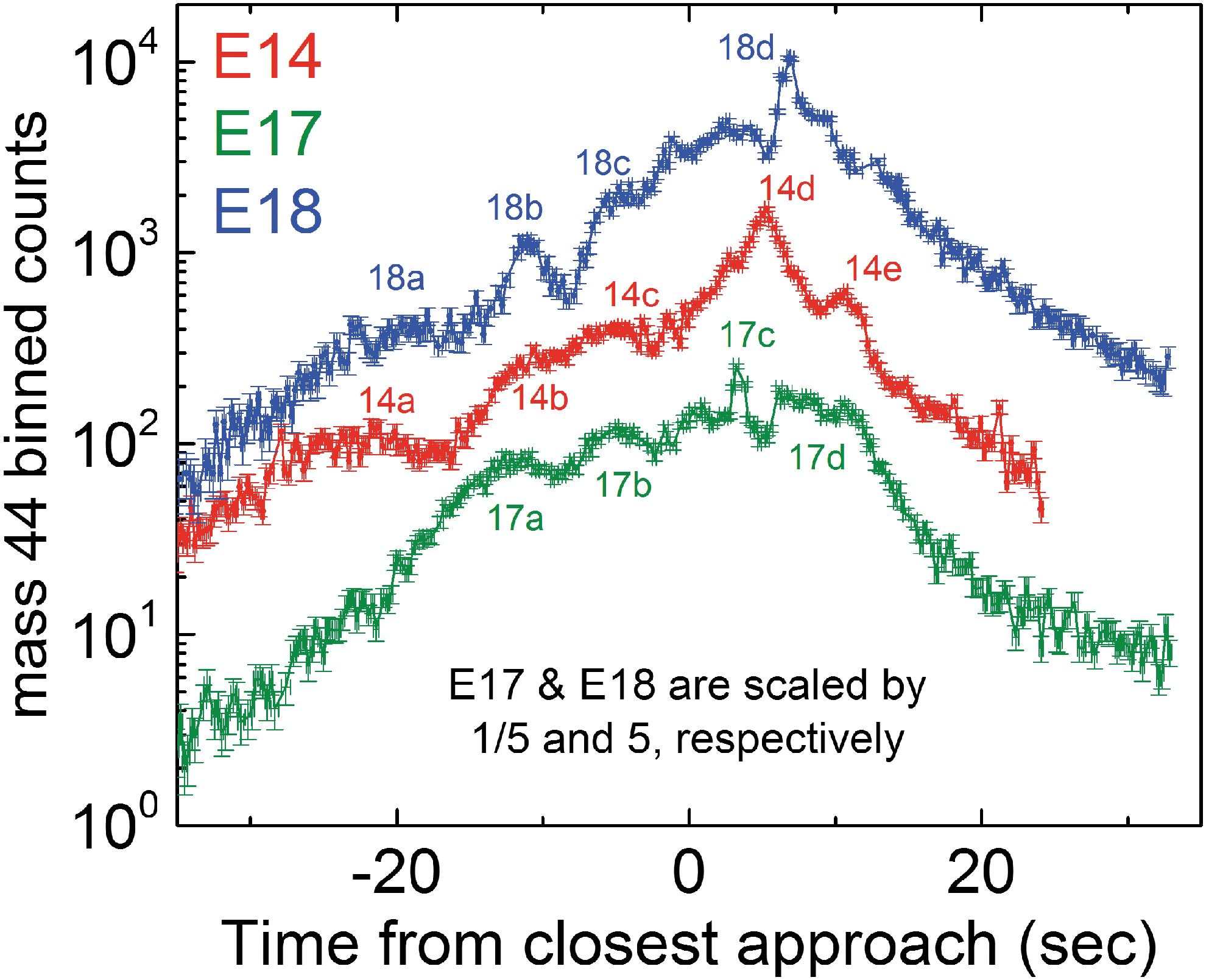
E14, E17, and E18 flyby data from the INMS mass 44 (CO2) channel (Perry et al., 2015) showing counts versus time from point of closest approach (approximately over the Enceladus south pole), showing (i) a broad region of high density corresponding to the diffuse plume, and (ii) individual peaks (several of which have been labeled) due to plume structure. Data too long after CA are not shown since postencounter residual gas in the instrument starts to dominate the signal. INMS, ion neutral mass spectrometer. Color images available online at
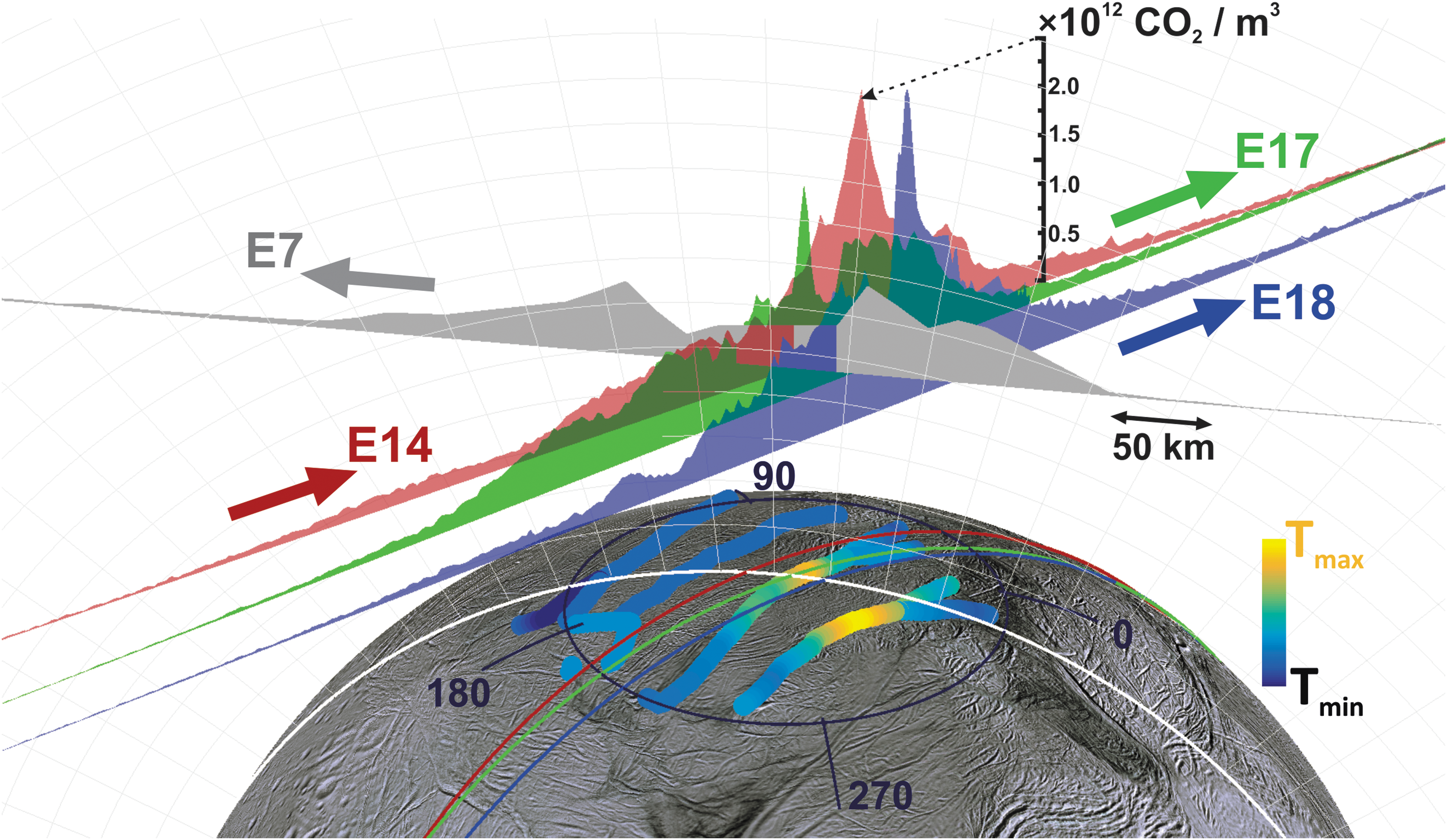
To scale 3D representation of the E14, 17, 18, and also (lower resolution) E7 INMS mass channel 44 data (Perry et al., 2015), with vertical areas representing (in linear scale) the CO2 density, and the flat base of the areas corresponding to the Cassini trajectories. Lines across the surface are the ground tracks. The tiger stripes are colored according to the relative temperature estimated by CIRS (Spencer et al., 2013). 3D, three-dimensional. Color images available online at
2. Analysis
Constraining the complete 3D plume structure solely on the basis of only a few INMS flybys is challenging, as multiple combinations of jet pointing directions and intensities can fit the data, and the jets may also be time variable. Time changing tidal stress fields in Enceladus' crust that act to open and close the surface fissures (Nimmo et al., 2014) and that are thought to drive the plume's orbital position-dependent time variability (Hedman et al., 2013) may also cause temporal changes in jet intensities unique to the individual jets, depending on local details of the subsurface fissure geometry beyond detectability. For many years, understanding of the jet 3D structure was limited to the preliminary imaging-based analysis of the grain jets by Spitale and Porco (2007) suggesting eight primary jet sources. Sufficient and high-resolution imaging data was eventually acquired to enable a more detailed analysis of the plume grain distribution, which suggested the presence of more than 98 individual jets, with a possible contribution of quasi-uniformly distributed interjet emission along the tiger stripes (Porco et al., 2014). Using an alternate model, Spitale et al. (2015) hypothesized that the eruptions predominately take the form of continuous curtains of material, with very few collimated jets. This alternative has since been refuted (Porco et al., 2015), but we address both models here. The grains are accelerated and carried in the vapor flow and, therefore, the locations and pointing directions (if not the spreading) of the vapor and imaged grain jets should coincide within tens of kilometers to the surface sources (the micron-sized grains decouple from the gas flow within 10 vent diameters, that is, within a few meters [Yeoh et al., 2015]). Accordingly, the locations and directions as determined by Porco et al. (2014) can, in principle, provide a major constraint on UVIS- and INMS-based plume modeling. Using the UVIS data, Portyankina et al. (2016) began modeling the plume with all 98 (Porco et al., 2014) jets, adopting a Monte Carlo modeling approach. Here, we combine UVIS with INMS observations to constrain the vapor emission intensity and velocity, assuming as sources, where applicable, the 98 particle jets, using an analytical modeling approach computationally efficient for analyzing such a large number of plume sources.
We approximate the gas velocity distribution as Maxwellian plus a source bulk velocity, which is computationally expedient since the gas density versus position n (r, θ, S, M, vM
) of such a drifted Maxwellian distribution (with r, θ, S, M, vM
the distance to source, angle from the jet axis, source flux, thermal Mach number, and gas thermal speed at the vent exit, respectively) is readily calculated with an analytical expression as applied by Dong et al. (2011) and Tenishev et al. (2014) (see Dong et al. [2011] for a full derivation):
where the thermal Mach number M = vb
/vM
is the ratio of bulk to thermal speed
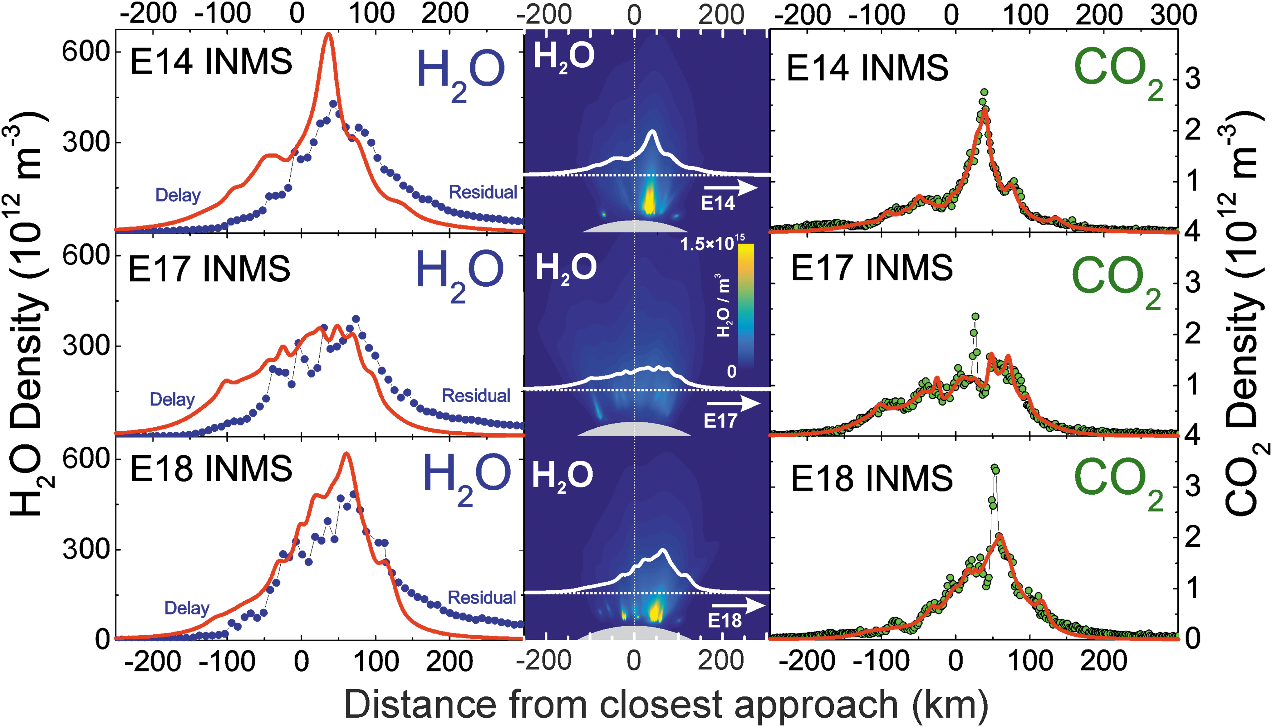
Right: model fits (red lines) to the INMS-measured CO2 densities (green points) versus distance along Cassini's trajectory, with the (Porco et al., 2014) jets as the constraint. Left: INMS-measured H2O densities (blue points), and the CO2-based model prediction for the H2O density (red line). The prediction takes into account the relative mixing ratios of CO2 (∼0.24%, 0.37%, and 0.24% at E14, 17, and 18) and H2O (∼90%) in the plume, and corrects for the anticipated (mCO2/mH2O)1/2 thermal Mach number mass dependence (Hurley et al., 2015; Perry et al., 2015). Measured and modeled H2O disagree due to H2O adsorption in the INMS, which distorts the signal by (1) delaying H2O transmission through the gas inlet to the ion source and (2) causing residual H2O to persist in the instrument even after Cassini has exited the plume. Center: model plume density cross sections for each flyby in the plane subtended by Cassini's trajectory (dotted line) about Enceladus' center, with the solid white lines (same as red lines on left) showing the model density profile versus position. Note that densities decrease near the surface since the plane shown cuts between tiger stripes and jets. Color images available online at
Our model considers two possible plume contributors: (1) an upward (normally) directed gas source continuously distributed along the tiger stripes, and (2) multiple jets at discrete tiger stripe locations. For a continuous source, the summation, Equation 1d, is formally an integration along the tiger stripes, which we approximate with many (350 in total) closely (2 km) spaced upward-directed jets along the tiger stripes as done by Tenishev et al. (2014). The continuous source, or the jets with locations/pointing from the work of Porco et al. (2014), are given a thermal Mach number distribution, as appropriate for gas emerging from a fissure with a distribution of flow velocity (e.g., slower near the walls [Tucker et al., 2015]). We use a four-point Mach number distribution from Mach 0, 2, 4, and 16, respectively; that is, a mixture of thermal isotopically expanding gas (Mach 0) to fast supersonic emission (Mach 16), as required to best fit the shapes of the features in the UVIS and INMS data (Fig. 10). We performed multiple model runs by varying each of the four Mach number contributions (i.e., a four-dimensional parameter space) and determined the relative source fluxes that provided the best fit to all of the (INMS and UVIS) flyby data sets. The best fit values are 18% (at Mach 0), 18% (at Mach 2), 52% (at Mach 4), and 12% (at Mach 16), with ∼±30% uncertainty on each contribution. The Mach numbers 0, 2, 4, and 16 apply to CO2; for H2O, we assume the bulk gas speed and temperature to be equilibrated with CO2 and, accordingly, scale the thermal Mach numbers down in inverse proportion to the (mass dependent) thermal velocity, that is, by (mH2O/mCO2)1/2 = 0.64 (Hurley et al., 2015; Perry et al., 2015). The Mach number distribution is described by the source flux weights CM
(Eq. 1d) for each Mach number, which we set to C
1 = 0.18, C
2 = 0.18, C
3 = 0.52, and C
4 = 0.12, as shown in Figure 10. These values feed into the expression for the total source rate S from the Enceladus plume:
The model is fit to each INMS or UVIS data set (Table 1) by varying the strength (i.e.,
3. Results and Interpretation
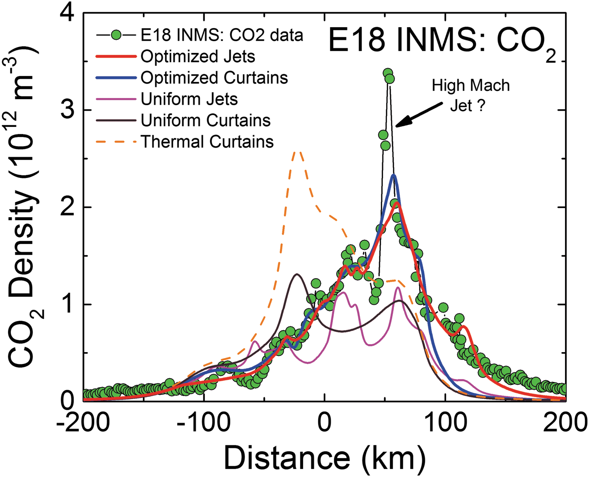
In Figures 3 –9, we compare two end-member models—the continuous emission and nominal 98-jet model—to the INMS E14, 17, and 18 CO2 density measurements and to the UVIS solar occultation H2O column density measurements, and we find that both models succeed in approximating the broad and the fine-scale structures (attributable to localized sources such as individual jets) observed in the gas densities. The gas distributions from the tiger stripes and jets are well blended at Cassini's altitude (e.g., 66 km E17, 18 flybys) due to the angular spread of the emission and, therefore, INMS is to a large degree measuring a summation over multiple tiger stripes and gas jets. We also show in Figure 3 the modeled H2O densities along the E14, 17, 18 trajectories, estimated on the basis of the model fits to CO2, after correcting for the relative mixing ratios of CO2 (0.4% ± 0.1%, depending on the flyby) and H2O (∼90%) and the molecular mass dependence (mH2O/mCO2)1/2 of the thermal Mach number (Hurley et al., 2015; Perry et al., 2015). The significant disagreement of the INMS H2O measurement with the model is due to H2O adsorption in the instrument, which distorts the signal by delaying the transmission of water vapor through the INMS (Teolis et al., 2010). Some features of the data are missed by both the continuous and the jet models, most notably the intense sharp peak in the E17 CO2 density (Figs. 3 and 8), and another at E18 (Figs. 3 and 9), possibly (though not likely) due to an ice grain impact in the INMS not filtered by the data analysis (Perry et al., 2015), or (more likely) due to Cassini directly intercepting individual high Mach number jets. These jets (1) may have been missed by our model as a result of the reported uncertainty (Porco et al., 2014) in the jet pointing directions, due to error inherent in the triangulation, together with a possible contribution of real jet directional variability, or (2) these may be unidentified jets missed by ISS imaging due to stochastic variability in their emission strength as discussed by Porco et al. (2014). Stochastic variability may result from clogged vents blowing open under the build-up of pressure, downward propagating cracks meeting a water-filled crack leading to a violent explosive outgassing, or pressure-driven fluid motion leading to boiling in tidally flexed cracks as discussed below. However, the nominal jet model captures some aspects that continuous emission does not, particularly the outbound CO2 tails in the E14, 17, and 18 INMS data (Figs. 3 and 7 –9). The tails are successfully fit with several of the high-angle (off-normally pointed) (Porco et al., 2014) jets, suggesting that a fraction of the plume gas is ejected (Porco et al., 2014) with significant off-normal bulk velocity components. A model consisting of only jets is sufficient to explain the data, provided the jet sources contain (in addition to the sharp high Mach number emissions) a component of slow, isotropic gas emission, as shown in Figure 10. However, the most plausible interpretation of the UVIS and INMS data is that the plume vapor distribution is at least partially attributable to jets, possibly mixed with continuous interjet emission along the tiger stripes. We reproduce Figure 12 from the work of Porco et al. (2014) showing the highest resolution (80 m/pixel) ISS image mosaic, in which it can be seen that a combination of both (1) numerous off-normal jets and (2) continuous sheets of interjet brightness due to faint particulate sheets most accurately describe the plume source.
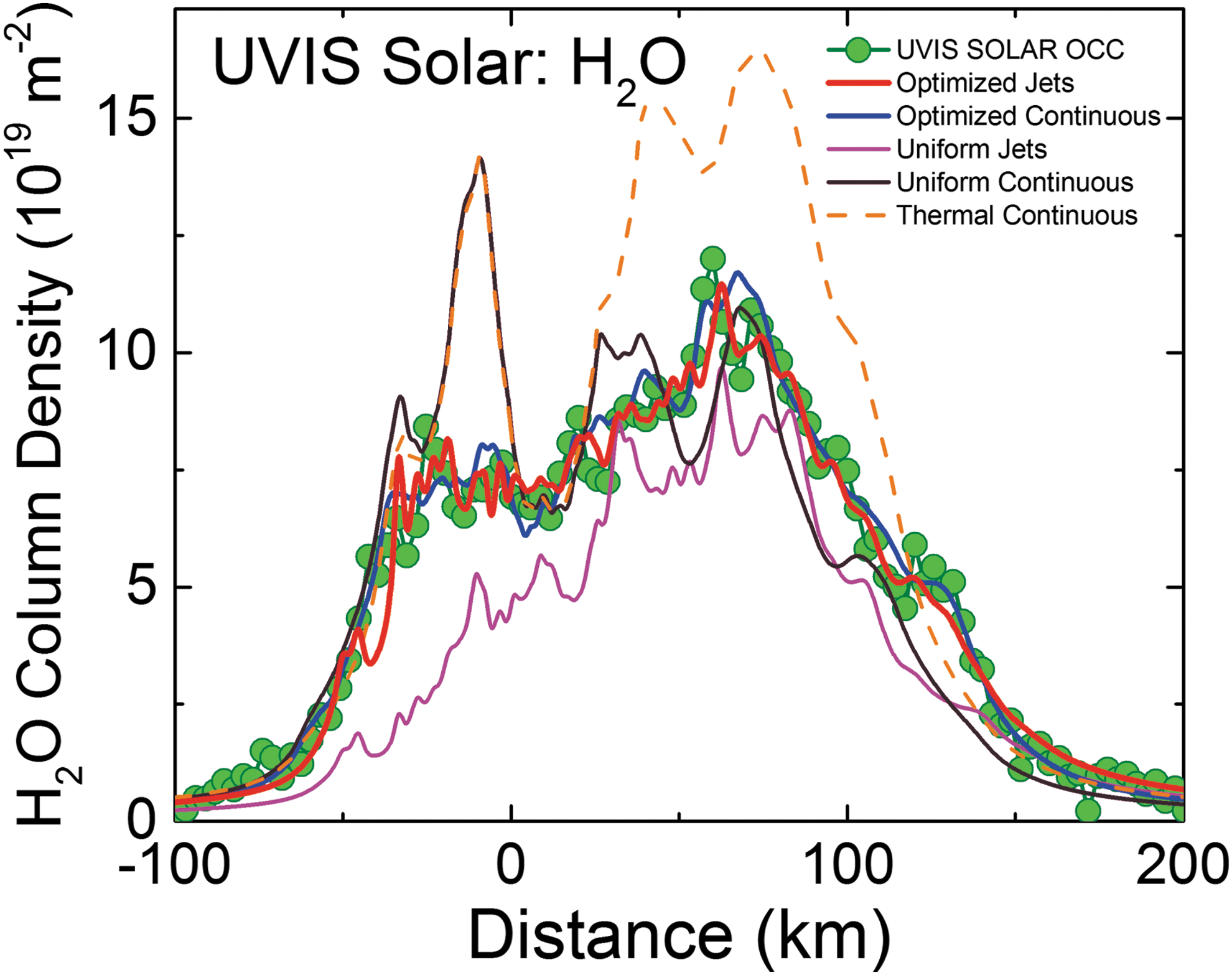
Enceladus plume water vapor column molecular number density measurement from the UVIS 2010 solar occultation (green circles). The x-axis origin is the point of closest approach (CA) of the line-of-sight to the sun to the limb of Enceladus (at 14 km altitude); x-axis gives the minimum distance of the line-of-sight from CA (time increases left to right, see also Figs. 5–6). We used the Hansen et al. (2011) calibration to estimate the H2O column density. Red line: average model solution for the optimized (Porco et al., 2014) jets. Blue line: average solution for continuous emission along the tiger stripes. Magenta line: jets with equal intensity. Brown line: uniformly distributed continuous curtain emission along the tiger stripes; this model predicts four large peaks coincident, from left to right, with the Alexandria, Cairo, Baghdad, and Damascus tiger stripes. Orange dashed line: continuous curtain emission with emission strength dependent on tiger stripe temperature (proportional in this example to Tn
, with n = 7). Color images available online at
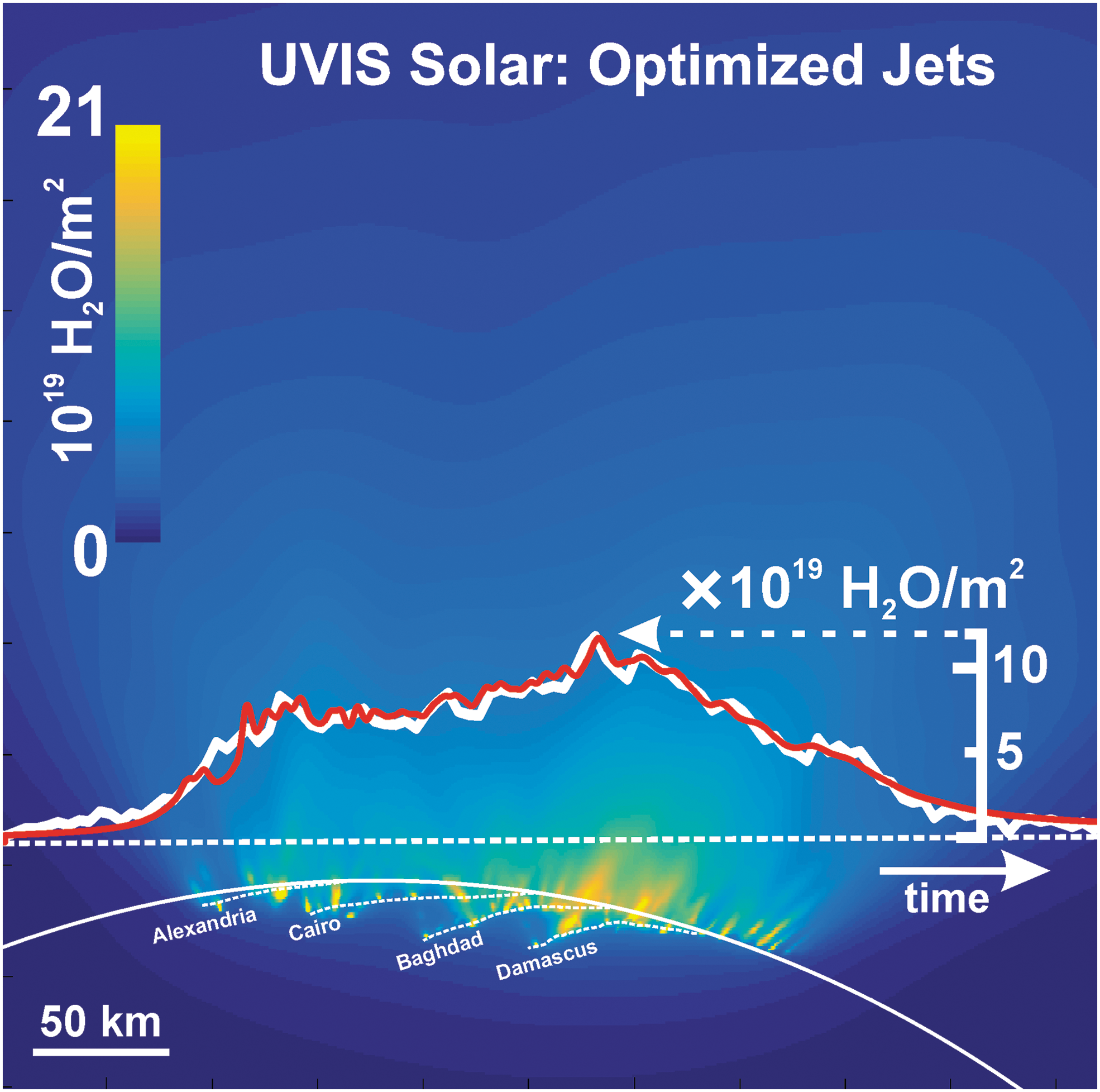
Modeled plume water vapor column density for the optimized (Porco et al., 2014) jets, as viewed along Cassini's line of sight to the sun during the UVIS 2010 solar occultation. Dashed line: line scanned by UVIS, versus time from left to right. White line: H2O column density profile measured by UVIS versus position along the scan line (see scale on right). Red line: modeled H2O column density profile versus position along the scan lines; note coincidence of peak positions with locations of jets along the scan line. Profiles are same as those in Figure 8. Color images available online at
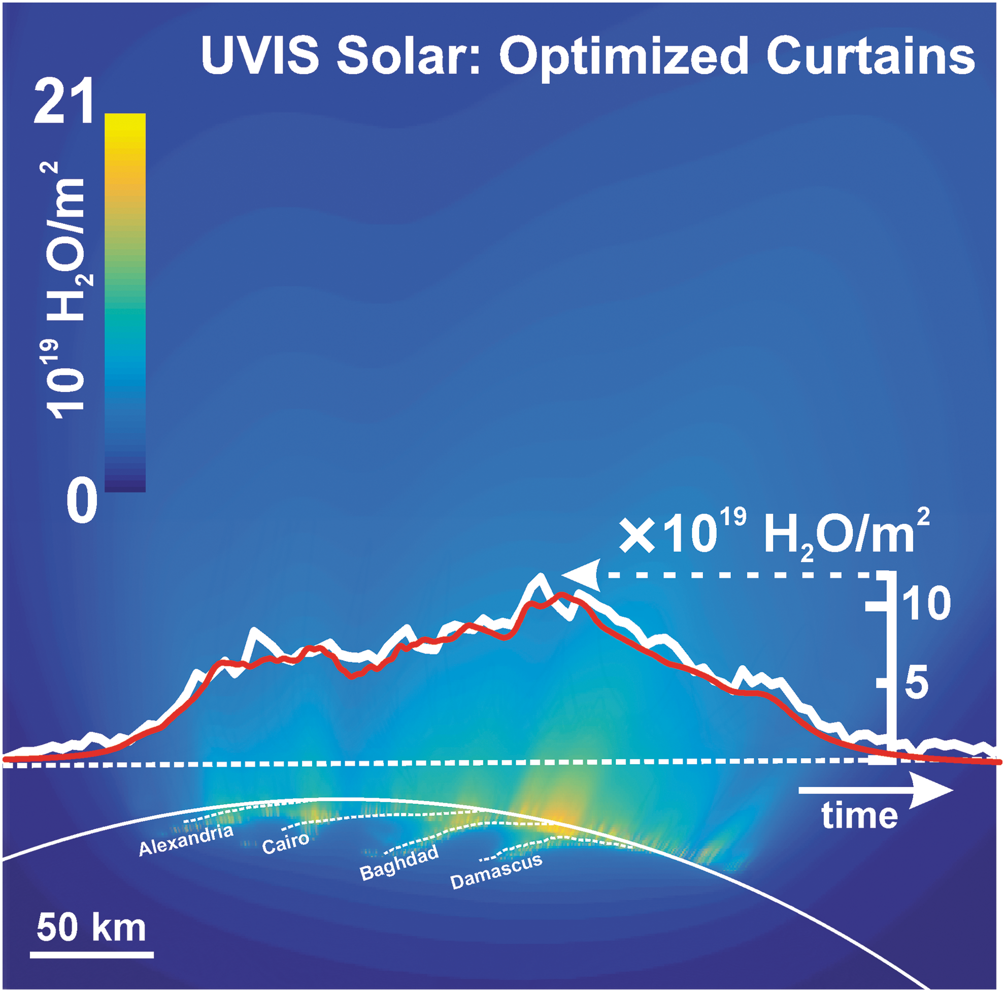
Same as Figure 5 for optimized continuous curtain emission along the tiger stripes, which we approximated by 350 closely (2 km) spaced upward-directed jets along the tiger stripes. Color images available online at
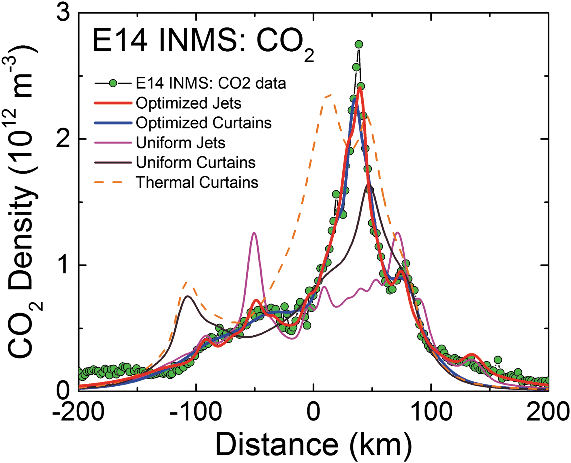
INMS CO2 molecular number density measurement (green circles) along the 90 km altitude E14 flyby trajectory showing structure in the along-track plume density. Results plotted versus distance from closest approach to Enceladus along Cassini's trajectory, with time increasing left to right. Red line: average model solution with the (Porco et al., 2014) jets as the constraint. Blue line: average solution for continuous emission along the tiger stripes. Magenta line: jets with equal intensity. Brown line: uniformly distributed continuous curtain emission along the tiger stripes. Orange dashed line: continuous curtain emission with emission strength dependent on tiger stripe temperature (proportional in this example to Tn
, with n = 7). We used the processed CO2 data from the work of Perry et al. (2015), and the updated INMS neutral density calibration model from the work of Teolis et al. (2015), to estimate the gas density. Note that the average CO2 mixing ratio is measured by INMS to be ∼0.24% in the plume (in terms of molecular density), with H2O vapor comprising most of the remaining gas (∼90%). Color images available online at
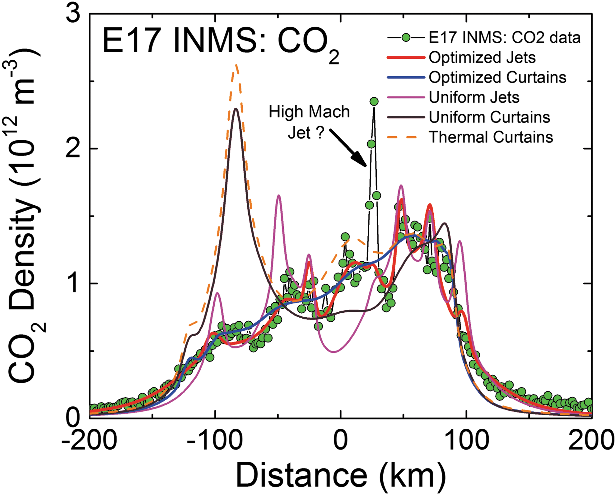
Same as Figure 7 for the 66 km altitude E17 flyby. The CO2 mixing ratio in the plume vapor is measured by INMS to be ∼0.37%. The sharp peak at ∼30 km past closest approach, not captured by the models, may be high Mach jet directly intercepted by Cassini, or (less likely) an ice grain impacting the instrument not filtered by the data processing (Perry et al., 2015). Color images available online at
Same as Figures 7and 8 for the 66 km altitude E18 flyby. The CO2 mixing ratio in the plume vapor is measured by INMS to be ∼0.24%. The sharp peak at ∼50 km past closest approach, not captured by the models, may be high Mach jet directly intercepted by Cassini, or (less likely) an ice grain impacting the instrument not filtered by the data processing (Perry et al., 2015). Color images available online at
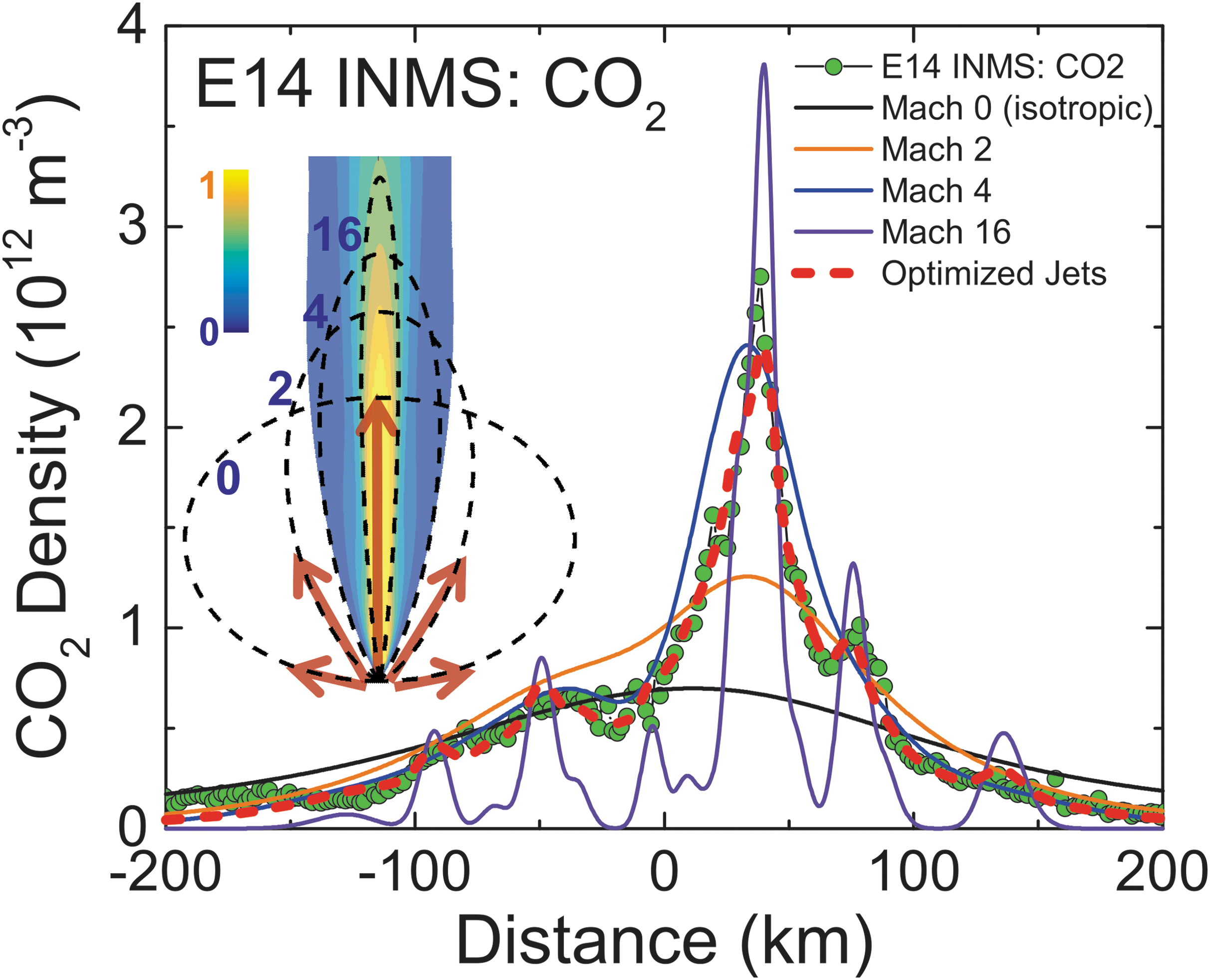
Example (with INMS E14 CO2 data: green points) showing why a Mach number distribution in the gas source is needed to fit data. Red dashed line: model fit using the (Porco et al., 2014) jets, assuming a distribution of Mach number in the normalized jet source flux (ΩM
= S/vM
, see text) with 18%, 18%, 52%, and 12% contributions from thermal Mach numbers 0, 2, 4, and 16, respectively. Solid lines: same model, except that all of the gas flux is at the given Mach number; black: 0, orange: 2, blue: 4, violet: 16. To aid in comparing the curves we have rescaled the Mach 0 and 16 curves by factors 3 and 0.5. Inset: schematic representation showing how the emission flux angular distributions (dashed lines) at different Mach numbers are summed to produce the modeled jet (density cross section contours shown, densities and dimensions to scale in relative units). Color images available online at
ISS high-resolution (400 m/pixel) image mosaic of the gas-propelled ice grain emission along the tiger stripes, showing the plume source to be characterized by numerous normally and non-normally pointed high Mach jets, together with sheets of continuous interjet emission. Note the near-surface brightness in between the jets just beyond (forward of) the terminator, indicating the presence of gas-propelled ice grains in both discrete and continuous, interjet, fissure-like eruptions. Figure reproduced from the work of Porco et al. (2014).
The mixture of both high and low Mach number components in the gas flux escaping the surface fissures, as implied by the UVIS and INMS data (Fig. 10), suggests that the emission may contain two contributions as follows: (1) fast vapor preaccelerated by the pressure gradient along the fissure length (or through nozzle-like throats within the fissure [Schmidt et al., 2008; Yeoh et al., 2015]) and (2) slow thermalized gas, which has either not undergone acceleration in the fissures (e.g., a near-surface liquid or solid [Goguen et al., 2013] sublimation source) or has been rethermalized by friction and/or thermal exchange with the fissure walls. The thermalized component is still at collisional densities of order 1021 molecules/m3 on emergence from the surface vent (Tucker et al., 2015) and thereby undergoes collisional expansion up to a few kilometers from the source (Yeoh et al., 2015). The millimeter gas mean free paths at the surface vent are shorter than the fissure widths, which are possibly tens of centimeters (Schmidt et al., 2008; Yeoh et al., 2015; Kite and Rubin, 2016), and thus the flow may segregate in the channel, with fast (cold) and slow (thermalized) vapor concentrated in the channel center and at a boundary layer near the fissure walls, respectively (Tucker et al., 2015). Gases such as CO2 measured by INMS are entrained in the water vapor flow, both near the walls and channel center, and thereby emerge from the fissures with bulk flow speed approximately equilibrated to that of the water vapor.
A limitation of the INMS (UVIS) gas density (column density) data is that it only provides constraints on the gas thermal Mach number, that is, the ratio of the bulk-to-thermal speed, whereas the gas bulk speed and temperature entering into the ratio are not constrained. The uncertainty is particularly acute in the high Mach number (fast) component of the emission, since it is not clear whether the gas is accelerated purely by passive adiabatic expansion of vapor from a static source (clathrates, or a stationary liquid reservoir at the H2O triple point; 611 Pa and 273 K), or whether the fluid acceleration is augmented by tidally driven compressional stress on the fissures (Kite and Rubin, 2016). Such stress would exert pressure on the fluid, which may flow in response both down into the subsurface ocean (if the fissure connects to the ocean) and transiently up toward the surface (if the fissure connects to the surface). A finite thickness at the top of the rising liquid column may boil as the pressure acting on the liquid falls below its vapor pressure (Porco et al., 2006; Ingersoll and Nakajima, 2016), drawing latent heat from the liquid to form ice near the triple point (possibly a gas-propelled mist of frozen droplets or grains). The gas/liquid/solid mixture may volumetrically expand nonadiabatically, with the expanding water vapor bubbles drawing heat from the liquid, while exerting (together with exsolving bubbles of other gas species: CO2, H2, NH3, or CH4 [Matson et al., 2012; Bouquet et al., 2015]) additional pressure to accelerate the fluid to high speed before arrival at the surface. For the baseline case of a static subsurface reservoir at the triple point, the gas is accelerated purely by the conversion of gas thermal energy to dynamic pressure as discussed by Yeoh et al. (2015) and is thus limited to a maximum ∼1 km/s ultimate adiabatic expansion speed at the fissure exit (Ingersoll and Pankine, 2010). However, if tidally driven flow and boiling also contribute to the acceleration, the speed may be much higher; for example, boiling liquid rising close to the surface may yield vapor escaping to space near 273 K, which (for Mach 16 × (18/44)1/2 ≈ 10 flow as seen by UVIS/INMS) implies a flow speed of ∼6 km/s. This translates to a ∼3 cm/s liquid flow speed in the fissures after dividing by the ∼2 × 10⁵ liquid-to-gas volume expansion factor; this is consistent with the required speed, ≥1.3 cm/s, for water to transit a 10 km thick ice shell (Thomas et al., 2016) within the freezing time scale (∼106 s for w ∼1 m, scales as fissure width squared [Porco et al., 2014]). This speed is a lower limit since some liquid freezes instead of vaporizing, and the remaining liquid may not have sufficient time to fully vaporize before exiting the vent. Hence, higher liquid flow speeds, for example, a few tens of centimeter per second as estimated by Kite and Rubin (2016) for 1 m fissures, could plausibly generate high-speed (∼6 km/s) jets with the thermal Mach numbers seen by UVIS and INMS. However, we note that the plume scale height appears constant in VIMS (with the possible exception of a small range of orbital position around apoapse) (Hedman et al., 2009) and ISS (Nimmo et al., 2014) images, not following the plume strength dependence on mean anomaly, which may be evidence that supports the adiabatic expansion scenario, that is, nozzle choked gas flow limited to the ∼1 km/s ultimate expansion speed, independent of source strength.
Accordingly, we have two limiting cases for the relationship of the gas thermal speed vM
exiting the vent to the thermal Mach number: (1) complete adiabatic expansion
obtained (see Gombosi [1994] Eq. 7.57, also Sutton and Biblarz [2001] Eqs. 3–12) from the definition M = vb
/vM
and by equating the total energy per molecule mvb
2/2 + mβvM
2/2 exiting the vent to the stagnation energy mβv0
2/2 of the subsurface vapor (here v0
= 565 m/s is the mean thermal speed of H2O at 273 K, and β = γ/(γ−1) = 4, with γ = 4/3 the water vapor heat capacity ratio); and (2) pure nonadiabatic acceleration (no expansional cooling):
Substituting into Equation 2 (and using the definition Σ
M
C
M
= 1), we obtain the adiabatic and nonadiabatic plume source rate estimates S
a and S
na:
where, using CM
= [0.18, 0.18, 0.52, 0.12] and M = [0, 2, 4, 16] × (mH2O/mCO2)1/2 for water molecules, we find S
a to be only ∼67% of S
na:
The plume source rate estimate therefore depends on the assumptions regarding the gas temperature and speed in the high Mach gas component of the plume. This is shown in Figure 11, where we plot the INMS- and UVIS-based plume source rate estimates versus Enceladus mean anomaly, for both the S = S a and S = S na limiting cases.
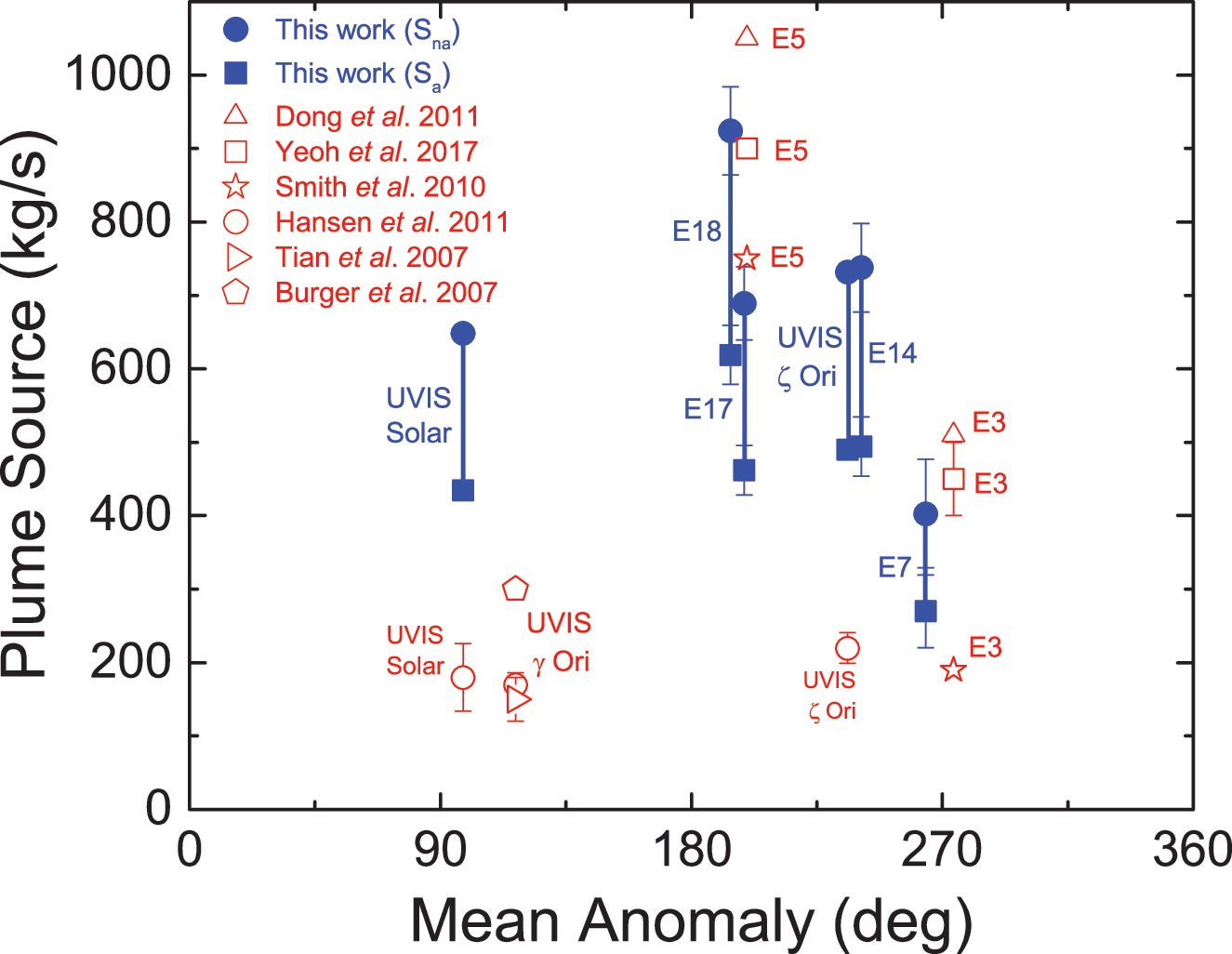
Total plume vapor mass source rates for the UVIS zeta Orionis and solar occultations, and the E14, E17, and E18 flybys, from our modeling (blue symbols), and for E3 and E5 from the works of Dong et al. (2011), Smith et al. (2010), and Yeoh et al. (2017), versus Enceladus mean anomaly at the time of the measurement. For our results, we show both Sna
(solid circles) and Sa
(solid squares) nonadiabatic and adiabatic upper and lower limiting source rates, and vertical lines to show the range of possible source rates. For the UVIS zeta Orionis and solar data, Hansen et al. (2011) used a 450 m/s gas speed (the H2O 170 K thermal speed) to estimate 220 and 180 kg/s source rates; our estimates are at least a factor two higher since our model requires significant high Mach gas flow. The source rate uncertainty and stochasticity, and the scarcity of measurements near periapsis, prevent us from conclusively identifying a mean anomaly trend. Color images available online at
We also contrast in Figures 4 and 7 –9 the continuous emission and jet models, optimized to fit the UVIS and INMS data, with three other (nonoptimized) models: (1) the Porco et al. (2014) jets with equal intensity, (2) continuous emission with uniform intensity along the tiger stripes, and (3) continuous emission correlated to the average tiger stripe temperature as estimated by the CIRS team (Spencer et al., 2013) from the radiated thermal brightness detected by CIRS versus position along the tiger stripes (Howett et al., 2011). As discussed by Spencer et al. (2013), the temperatures and widths of the endogenic tiger stripe emission (modeled with a wide low-temperature Tl , and a narrow high-temperature component TH , as continuous “bands” along the tiger stripes [Spencer et al., 2013]) are optimized to best match the stripe's infrared thermal emission spectra. The most extensive spatial coverage (obtained in March 2008 [Howett et al., 2011]) of the tiger stripes by CIRS FP3 (600–1100 cm−1) and FP4 (1100–1400 cm−1) is used. The FP3/4 sensitivity only allows for constraints on the high-temperature endogenic component and, therefore, the low-temperature component is constrained by a CIRS FP1 (10–600 cm−1) scan across Damascus, Baghdad, and Cairo obtained in August 2010 (Spencer et al., 2013) (their Fig. 1). Since the CIRS spatial resolution does not permit identification of discrete hot spots in most of the tiger stripe system, this model is best suited to modeling a background of continuous or diffuse gas emission along the tiger stripes, rather than individual jets. Our approach was to define an empirical relationship positively correlating gas source rate to the temperature TH (i.e., the high-temperature component, presumably concentrated at the vents), then to adjust parameters to determine whether a fit to the data was possible (as an example we show a power law relationship in Figures 4, and 7 –9).
We found (Figs. 4 and 7 –9) that no choice of functional relationship of source rate to temperature provided a good fit to the observations. Although warm fluid flow (gas and/or liquid) through the fissures is a plausible explanation for surface heating around the surface vents (Matson et al., 2012) (whether by condensation latent heat or direct conduction to the walls), the thermal inertia of the surface material (≥27 Jm−2Ks−1/2 [Howett et al., 2011]) may make the surface temperatures around the vents unresponsive to rapid change (on the order of hours or less) in local emission strength. Therefore, irrespective of the correlation of tiger stripe temperatures to the time-averaged plume activity (Porco et al., 2014), the tiger stripe temperatures may not well approximate the local emission strength at any given moment. Additionally, the relationship of temperature and gas flux may be a function of geometrical considerations at the vent. For a tidally flexed planar fracture, it is possible the fluid flux could vary proportionally to the fracture width, a result consistent with choked gas flow, leaving the contact area between the gas and the fracture wall (and thereby the heat flux) independent of width.
As can be seen by comparing the 3D projections of Figures 13 –16, our model results suggest drastic time variability in the plume sources along the tiger stripes. Using the Porco et al. (2014) jets as the modeling constraint, the model allows, in some cases, identification of specific jets that may have changed between flybys. An example is jets 37 and 59 from the work of Porco et al. (2014); only these jets have the required location and direction to fit the major peak in the E14 CO2 density, suggesting enhanced activity from these jets during E14 (Fig. 14), with source rates ∼10 and ∼12 kg/s, respectively (significantly above the average ∼1.5 kg/s intensity of the other jets). At these intensities, however, jets 37 and 59 would contribute too much signal to the E17 model, that is, the model fit to the E17 data requires these jets to be at low intensity during the flyby (Fig. 15). Many vapor jets appear to change drastically and stochastically between flybys, showing no discernible correlation to the nominal jet sightings in ISS images, or their proxy intensities as reported by Porco et al. (2014). This could be due to inherent and even expected changes, either in the strength or the direction of the jets, between the times the various instruments made their observations. As can be seen in Figure 11, the total plume source rate also exhibits substantial stochastic variability, up to a factor ∼5 between measurements, and most of the measurements are clustered in a small range of mean anomaly just past 180° apoapsis, making any systematic mean anomaly dependence in the vapor emission difficult to discern.
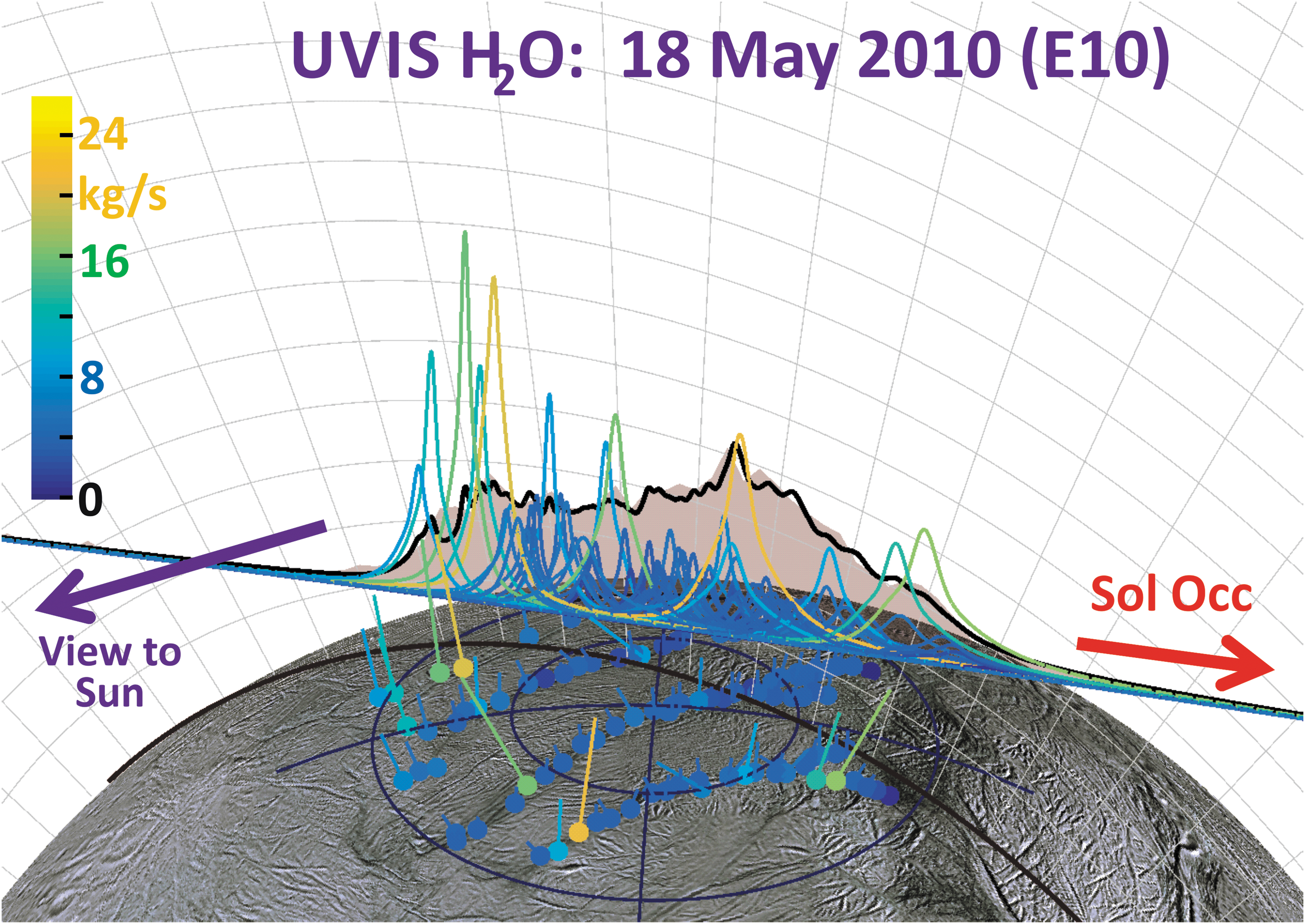
To scale 3D representation of the 2010 Enceladus plume UVIS Solar Occultation with vertical areas representing (in linear scale) the occulted intensity fraction (corresponding to the water vapor column density), and the flat base of the area corresponding to the line of minimum ray height (brown line on surface is the “ground track” of this ray). Cassini's viewpoint onto the plume is from the upper right of the figure, and UVIS is scanned from left to right as shown by the arrow. Dots on surface: (Porco et al., 2014) jet source locations, with straight lines showing jet directions. The colors and jet line lengths are given by the optimized jet strength: orange (blue), long (short) jets represent high (low)-intensity jets. Color bar scale: estimated jet source rates in kilograms per second. Colored curves: line height gives the estimated column density profile of each jet along the UVIS line of sight. Black curve: the best fit total column density after summing the contributions of all jets. Color images available online at
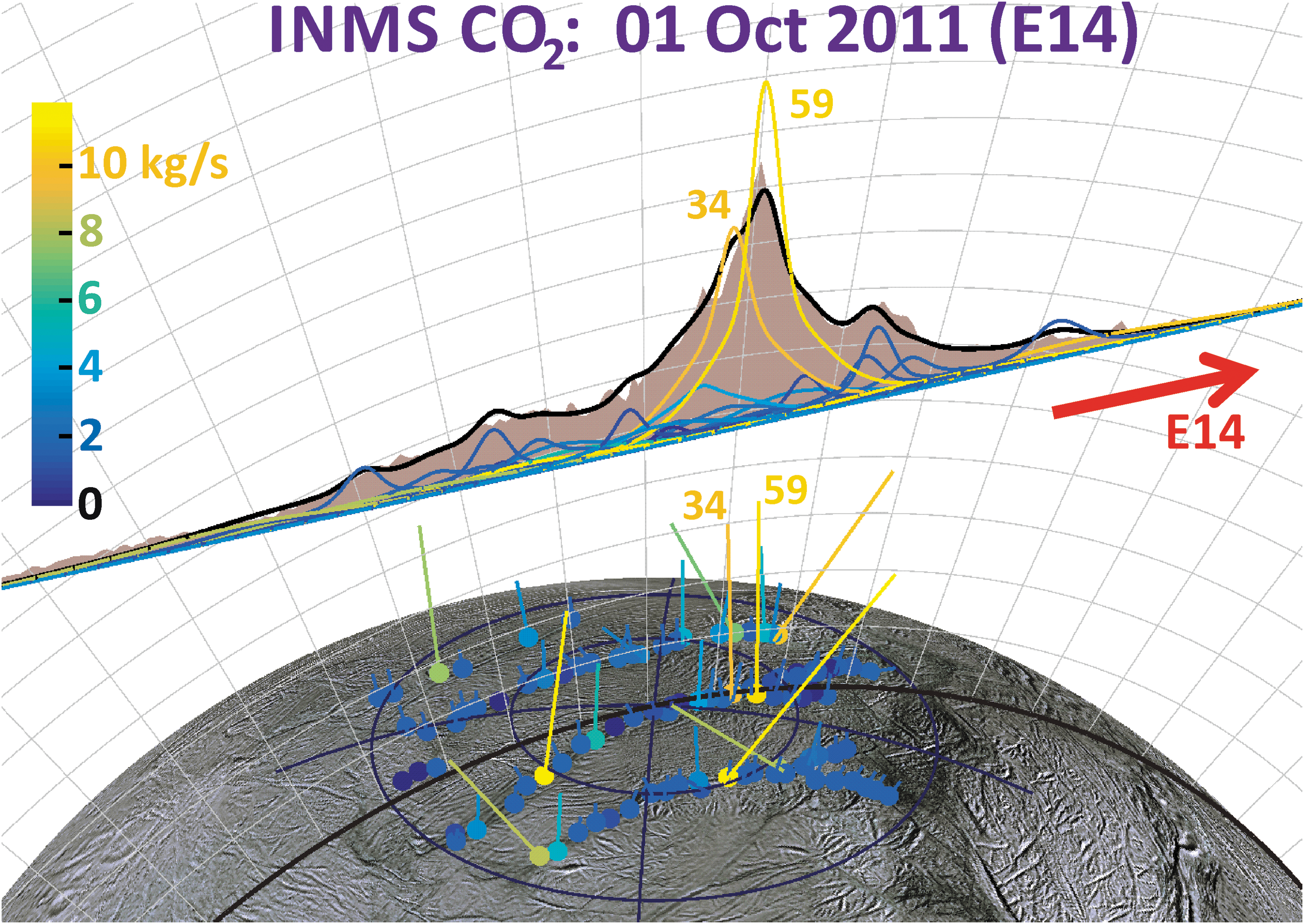
To scale 3D representation of the INMS CO2 data from the 90 km E14 flyby, with vertical areas representing (in linear scale) the mass 44 CO2 signal (corresponding to the CO2 gas density), and the flat base of the area corresponding to Cassini's trajectory (red arrow shows spacecraft direction, brown line on surface is the ground track). Dots on surface: (Porco et al., 2014) jet source locations, with straight lines showing jet directions. The colors and jet line lengths are given by the optimized jet strength: orange (blue), long (short) jets represent high (low)-intensity jets. Color bar scale: estimated jet source rates in kilograms per second, renormalized to correct for the measured 0.24% CO2 mixing ratio in the plume. Colored curves: line height gives the estimated density profile of each jet along the E14 trajectory. Black curve: the best fit total column density after summing the contributions of all jets. The model suggests enhanced emission from jets 34 and 59 (Porco et al., 2014) elevated activity, as these are the only jets with the required location and pointing to fit the intense CO2 density maximum. Color images available online at
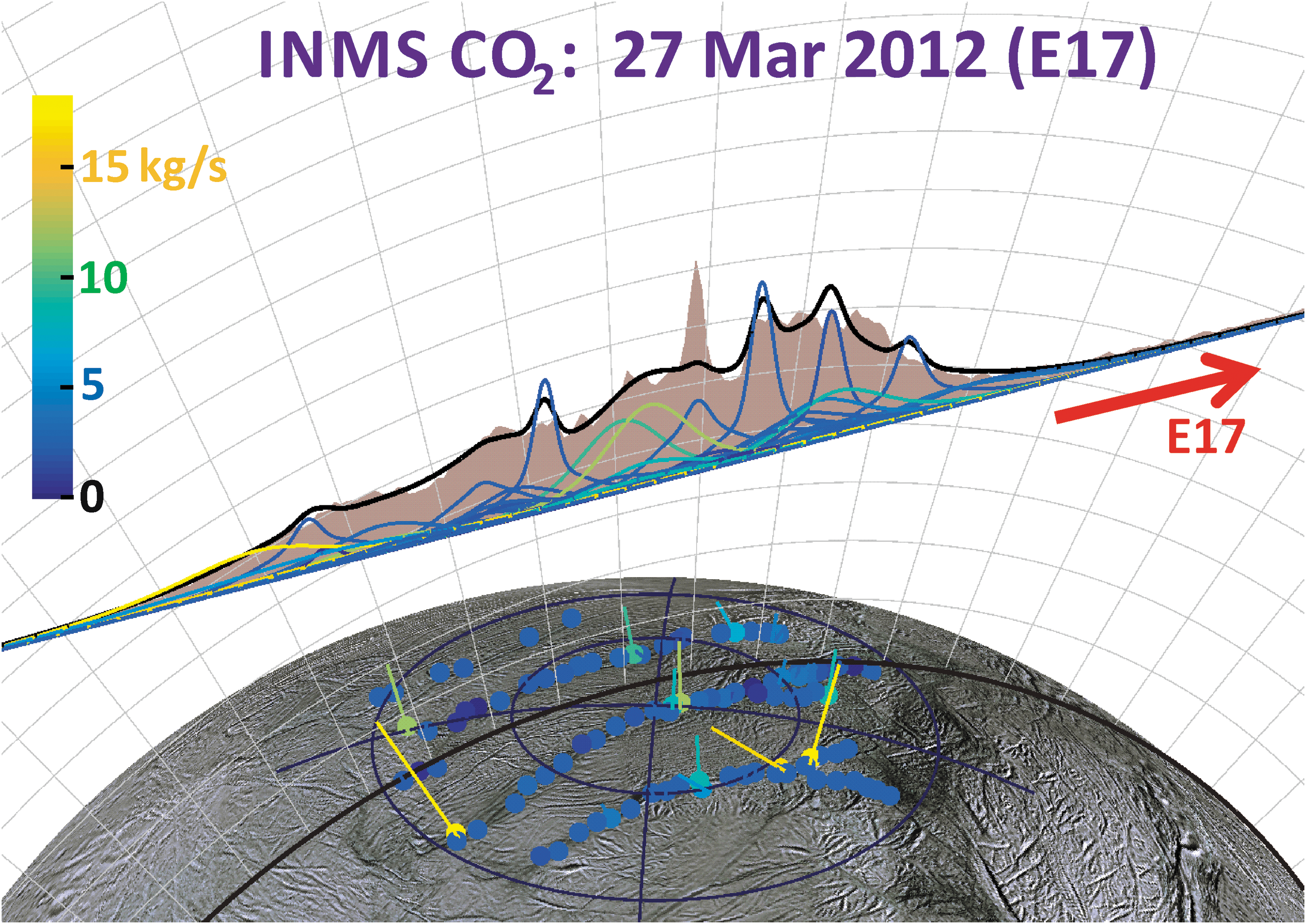
Same as Figure 14 for the 66 km altitude E17 flyby. Color images available online at
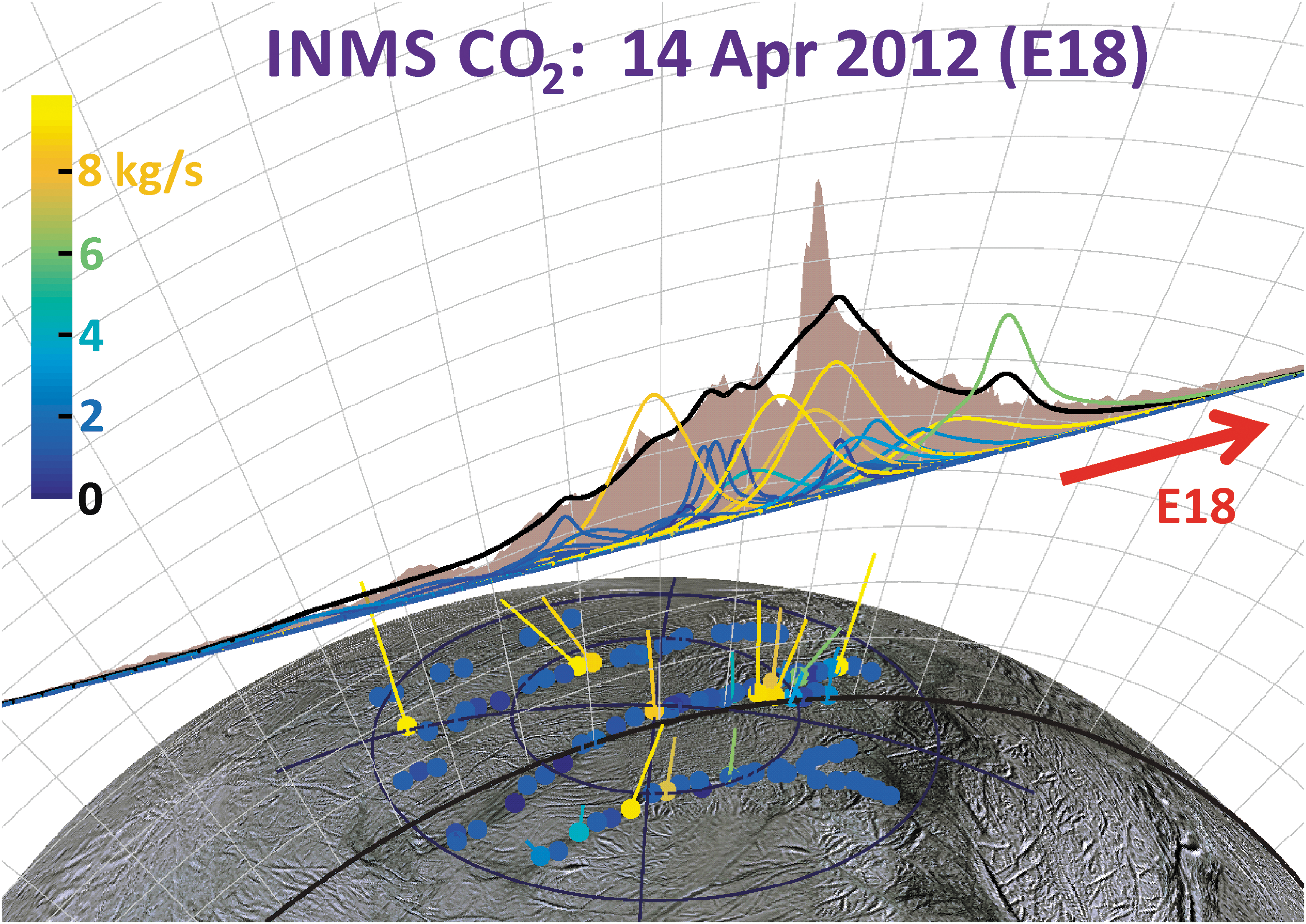
Same as Figures 14 and 15 for the 66 km altitude E18 flyby. Color images available online at
4. Conclusions
The Cassini spacecraft's multiple low-altitude traversals through the Enceladus plume, and the direct capture and high-cadence analysis of gas intercepted by INMS along the spacecraft trajectory, have revealed in high resolution the structurally complex and dynamic vapor cloud emanating from discrete plume sources (tiger stripes, geysers). The extraction from INMS of plume densities, both for minor species and for sticky water vapor, has proved to be a major challenge, spanning many years and multiple flyby attempts and requiring the development of new instrument calibration models (Teolis et al., 2015) and data analysis methods (Teolis et al., 2010; Perry et al., 2015). On the basis of the INMS data, in combination with UVIS stellar and solar occultation measurements of the vapor column density through the entire thickness of the plume, our models reveal that the plume's vapor distribution requires both low and high Mach emission from the surface sources, a result consistent with a mix of (1) high-speed gas emission (e.g., thermal expansion of gas through nozzle-like channels or boiling/pressure-driven acceleration in narrow fissures) and (2) low-speed thermal emission, such as a near surface solid or liquid sublimation source or a thermalized gas layer in contact with the fissure walls. The INMS and UVIS data suggest the presence of multiple discrete and off-normal gas jets, likely combined with continuous interjet emission, a finding consistent with high-resolution images (Porco et al., 2014) (Fig. 12). Combined with observations acquired along closely spaced trajectories but at different times, the modeling also implies drastic and stochastic time variability of the individual gas jets and/or distribution of emission along the tiger stripes, consistent with ISS indications of stochastically time-variable jets (Porco et al., 2014). The total plume intensity, between 100 and 1000 kg/s, is also stochastically variable between Cassini flybys in UVIS and INMS observations, and estimates of the source rate are dependent (by up to ∼30%) on the assumed temperature and speed of the high Mach emission, as determined by the roles of adiabatic and nonadiabatic fluid expansion in accelerating the gas. The confirmation by multiple Cassini instruments of such intricate structure and dynamics in the Enceladus plume is a seminal accomplishment of Cassini's decade-long exploration of this active world, and a compelling basis upon which to elucidate, by way of earth-based studies and future spacecraft exploration, the origin and physics of the Enceladus plume and its physical and compositional relationship to the subsurface ocean.
Footnotes
Acknowledgments
This research was supported by the NASA Cassini Data Analysis and Participating Scientists Program under Grant No. NNX14AD41G.
Author Disclosure Statement
No competing financial interests exist.