
Abstract
We present a framework for studying generic behaviors possible in the interaction between a resource-harvesting technological civilization (an exo-civilization) and the planetary environment in which it evolves. Using methods from dynamical systems theory, we introduce and analyze a suite of simple equations modeling a population which consumes resources for the purpose of running a technological civilization and the feedback those resources drive on the state of the host planet. The feedbacks can drive the planet away from the initial state the civilization originated in and into domains that are detrimental to its sustainability. Our models conceptualize the problem primarily in terms of feedbacks from the resource use onto the coupled planetary systems. In addition, we also model the population growth advantages gained via the harvesting of these resources. We present three models of increasing complexity: (1) Civilization-planetary interaction with a single resource; (2) Civilization-planetary interaction with two resources each of which has a different level of planetary system feedback; (3) Civilization-planetary interaction with two resources and nonlinear planetary feedback (i.e., runaways). All three models show distinct classes of exo-civilization trajectories. We find smooth entries into long-term, “sustainable” steady states. We also find population booms followed by various levels of “die-off.” Finally, we also observe rapid “collapse” trajectories for which the population approaches n = 0. Our results are part of a program for developing an “Astrobiology of the Anthropocene” in which questions of sustainability, centered on the coupled Earth-system, can be seen in their proper astronomical/planetary context. We conclude by discussing the implications of our results for both the coupled Earth system and for the consideration of exo-civilizations across cosmic history. Key Words: Anthropocene—Astrobiology—Civilization—Dynamical system theory—Exoplanets—Population dynamics. Astrobiology 18, 503–518.
1. Introduction
S
But is the situation on Earth unique? In particular, given its global scale, might the transition represented by the Anthropocene be a generic feature of any planet evolving a species that intensively harvests resources for the development of a technological civilization? With the advent of reflex-motion and transit-based exoplanet searches, it is now apparent that most stars harbor families of planets (Seager, 2013). Indeed, many of those planets will be in the stars' habitable zones (Dressing and Charbonneau, 2013; Howard, 2013).
In Frank and Sullivan (2016), the results of exoplanet studies were used to set an empirical limit on the probability that Earth was the only world in cosmic history where such an energy-harvesting species evolved. Their result showed that, unless the probability per habitable zone planet for such “exo-civilization” evolution (P
c) was P
c < 10−22, Earth is not unique. Even if, for example, P
c were as low as 10−19, the number of technological civilizations like our own across the history of the visible Universe would still be large enough (N
c ∼ 1000) for statistically meaningful average properties of exo-civilizations to exist. These average properties include
While there is, of course, no data yet concerning exo-civilizations, our understanding of coupled planetary systems (atmosphere, hydrospheres, cryospheres, lithospheres, and possibly biospheres) has advanced considerably. Studies of Earth and other solar system bodies reveal a host of processes which can be expected to be generic on any planet (Alberti, 2016). Studies of Earth's geological record show a long interaction between the biosphere and other coupled systems which provide a foundation for physicochemical constrained generalizations (Gaidos and Knoll, 2012). Thus, much like physicists extrapolate known laws to explore consequences of new particles, astrobiologists can use what is known from Earth and solar system studies to explore the consequences of an exo-civilization's interaction with its own coupled planetary systems. This can be done by focusing solely on feedbacks from the resources the exo-civilization consumes and eliminating speculation over sociological factors by bundling “choices” into a few well-defined model parameters.
We take a dynamical systems approach to begin the development of such models. Specifically, we are interested in understanding the generic properties of trajectories for an energy-harvesting species developing a global-scale civilization that generates significant forcing/feedback on its host planet. This initial study is intended as a first exploration of such a dynamical systems approach. To this end we formulate and explore a suite of particularly simplified, low-dimensional models. Our family of models is intended to capture the basic features of a population n interacting with a planetary systems environment e through the consumption of some set of resources with different levels of environmental feedback.
We note that our study builds off of, and has similar concerns to, work in a number of fields such as population biology and population ecology. Our study also includes ideas that can be found in the field of ecological economics and work by authors such as Herman E. Daly and N. Georgescu-Roegen. Ecological economics shares our concern with planetary issues of energy use and sustainability, though in that field the concern is solely terrestrial (Costanza et al., 1997). Such issues were also explored in The Limits to Growth (Meadows et al., 1972). We recommend as well the particularly cogent earlier works exploring the Anthropocene from a broader planetary/astrobiological perspective that can be found in Schellnhuber and Wenzel (1998).
We have explicitly designed the models to remove all consideration of exo-civilization sociology. Our goal is to reduce the problem to its basic physicochemical and population-ecological roots with all consideration of agency reduced to simple inputs. In particular there is only a limited set of parameters in our model associated with the civilization's decisions. Since these parameters are set as inputs, they can be sampled randomly. There is no place in the models where we ask about the social dynamics of the decisions. We are not modeling the nature of the decision-making process or dynamics of the societal structures that determine the final decision. In principle our model could be applied to a biosphere with no civilization but with a certain class of feedbacks within the planetary systems. The strong coupling between the evolution of biospheres and other planetary systems is, for example, explored in the context of the evolution of habitability (Chopra and Lineweaver, 2016). When it comes to exo-civilizations, however, it is precisely this emphasis on basic physiochemical and population ecology principles that constitutes the innovation of our approach. We ask questions about exo-civilizations that can be constrained in similar ways that constrain questions about exo-biospheres.
Finally, it should be mentioned that there is a long tradition in astrobiology of using simple mathematical models to explore key issues in both a qualitative and quantitative manner (Jones, 1976; Newman and Sagan, 1981; Landis, 1998). Our work seeks to extend this tradition in a way that also provides some insights into the questions facing human civilization at the advent of its Anthropocene. The use of such models also has a history in the study of the Earth system as in the example of the Daisyworld model (Watson and Lovelock, 1983).
We begin in Section 2 with a description of our approach via population biological concepts and their application to the specific case of Easter Island. In Section 3 we introduce our modeling framework via a pair of basic ordinary differential equations (ODEs) that serves as the basis for all that follows. In Section 4 we present Model 1 representing civilization-planetary interactions via a single resource. In Section 5 we present Model 2 for civilization-planetary interactions with two resources that have different planetary system feedback. Section 6 explores Model 3 for a civilization-planetary interaction with two resources and nonlinear planetary feedback (i.e., runaways). Finally, in Section 7 we present our conclusions and indicate future directions for research.
2. Population Biology, Exo-Civilizations, and the Example of Easter Island
A full treatment of a resource-intensive civilization and its feedback on the host planet will require comprehensive simulations such as those provided by general circulation models (GCMs). GCMs are already being used to explore exoplanets with alternative exo-biospheres (Way et al., 2017). Thus their application to exo-civilizations would represent a natural extension. Given their complexity and cost to run, however, it is worthwhile to begin the exploration with simpler, lower-dimensional models (i.e., ODEs rather than partial differential equations). We note that the eventual inclusion of spatial inhomogeneity in the models may demonstrate interesting new effects such as when spatial diffusion is included in reactive systems. Local spatial imbalances could produce inverse cascades that feedback up to larger scales.
Population biology offers a natural starting point for our explorations since it has a long history of modeling nonlinear interactions among species and their environment. Predator-prey models, models of competition, and models of combat can be used. In particular, the logistic equation for the growth of population n is the classic “0-D” representation (no spatial dependencies) of a population's evolution (Kot, 2011),
where A is the growth rate of the species and K is the carrying capacity of the environment. Populations following the logistic equation show a characteristic S-shaped growth curve. The population initially rises as n ∝ eAt only to flatten out at n = K. The fact that the logistic equation predicts populations equilibrating at the carrying capacity K implies natural levels of resources are available to the species which need not be tracked. More complete models attempt to account for the availability of resources. These models show more complicated behavior for the population including the possibility of collapse or of limit cycles (Kot, 2011).
Such models can also be adapted to questions of the coupled evolution between human civilizations and their environments (Reuveny, 2012; Peretto and Valente, 2015). Easter Island presents a particularly useful example for our own purposes since it is often taken as a lesson for global sustainability (Brander and Taylor, 1998; Bologna and Flores, 2008).
Easter Island is surrounded by more than 1000 miles of ocean in all directions. As described by Basener and Ross (2005), the island was colonized between 400 and 700 AD by a small group of at most 150 humans. Sometime between 1200 and 1500 AD, the population grew to approximately 10,000, and the inhabitants built a culture that was artistically and technologically sophisticated enough to construct and transport their iconic stone statues. While there remains debate about the details of its history, many studies indicate that Easter Island's inhabitants depleted their resources, leading to starvation and termination of the island's civilization (Reuveny, 2012; Rull, 2016).
In the work of Basener and Ross (2005), a model for Easter Island tracked both the population n and a resource r directly related to the island's human carrying capacity (see also Safuan et al., 2012).
In this model the resource is renewable and has its own carrying capacity k. In addition, the resource has an additional “death rate” or sink in the form of human consumption governed by the parameter H. This model captured the qualitative rise and fall of Easter Island's population as it overshot the carrying capacity provided by the island's resources. While the results of Eq. 3 drive too rapid a collapse of the population to fully fit the data for the explicit case of Easter Island, they do provide us with a starting point for our own attempts to develop models capturing the coupled interaction of a species with its environment. In our case, however, the environment represents the physicochemical state of a planet's coupled systems. In the next section we introduce the underlying method and assumptions in our approach via a zeroth-order model.
3. Method
To explicate our approach, let us begin with what might be considered Model 0. These equations will form the basis for all that follows. We first assume the most basic dependence of the population on its environment expressed through the use of the logistic equation for the population with a growth rate A, and an environmentally dependent carrying capacity K(e). In addition, we assume the environment has a natural recovery rate C (see Table 1 for model parameters and their meanings).
In this approach we assume e = 0 is the “natural” state for the environment, with the action of the recovery term Ce bringing the planet back to that state. Note also that e c is the critical value of the environment. This defines the edge of “habitability” for the civilization on the planet such that the carrying capacity K(e) → 0 when e → e c. We note that the formal question of the singularity at K(e) = 0 has been discussed before (Kot, 2011; Safuan et al., 2012) and does not affect the solutions we discuss in what follows.
Note that unlike the model described by Eq. 3 we do not consider the planetary environment to be a resource. Instead we will consider the young civilization to have resources at its disposal which affect the state of the host planetary systems. The effect of the resource will appear in the equations when we add terms for additional “birth benefits.” These come to the population by using the resource. We will also add a “consumption detriment” that models the impact of the resource use on the planetary systems. In what follows, however, we will not explicitly track the time-history of the resource. It may be renewable or not, but for our purposes we consider the resource supply to be infinite. It will be useful in future studies to relax this assumption.
It is also possible that the changes in the planetary environment driven by the civilization might make it more difficult to obtain and use that resource. For example, the extraction of power via wind can alter available free energy in the global circulation, which in turn can disrupt (and therefore reduce) the available wind energy. For instance, it has been demonstrated that large-scale extraction of wind energy from the Earth system would, in fact, deplete this resource as laminar flows are converted into turbulent downstream flows (Miller et al., 2011). As with the case of following resource levels discussed above, we hope to explore these effects in future models.
Our method will follow a classic dynamical systems analysis for the extensions of Model 0. We will first look for equilibria, (n *, e *), in the system of equations. These are determined by the intersection of the “nullclines” of the system given by dn/dt = 0 and de/dt = 0. Once the equilibria have been found, we next determine their stability (by calculating the eigenvalues of their Jacobians). The equilibria may be stable or unstable in a variety of ways leading to solution trajectories that flow or spiral toward or away from (n *, e *). Limits cycles, in which the solutions circulate around the equilibria, are also possible.
In this study we are most interested in the nature of the trajectories for the population. Our questions can be summarized as follows: Under what conditions do the models lead to sustainable trajectories for the civilization (i.e., its population)? By sustainable we mean the ability to maintain a significant population for long times: n
* >> n
o where n
o ∼ 0. Under what conditions do the models lead to trajectories in which the civilization suffers significant overshoot before reaching n
*? By this we mean n
* < fn
peak where f is a number less than 1. We assume that a large die-off (small enough f) will represent a catastrophic event in the history of the civilization. Under what conditions do the equilibria lie in environmentally unstable domains? In our models the carrying capacity K(e) goes to 0 as e approaches e
c. Thus e ∼ e
c is an inherently dangerous regime for the planetary systems relevant to the civilization. The feedback making the planetary environment uninhabitable for the civilizations is likely to contain multiple nonlinear feedbacks that are beyond the current models to describe (though Model 3 contains a simple version of such feedbacks). Thus equilibria where e
* ∼ e
c can be considered dangerous for the long-term sustainability of the population. We therefore consider high n
* and low e
*/e
c to be favorable outcomes of the civilization–planetary systems coevolution. Under what conditions do the models lead to collapse trajectories for the civilization? Collapse implies a rapid evolution to n = 0. Note this may occur because the equilibria of the system has n
* = 0 and e
* ∼ e
c, or it may mean that no equilibria exist and populations head toward n → 0 and e → ∞.
4. Model 1: Civilization–Planetary System Interaction via Single Resource
We now add terms to the model representing consumption of a resource (of infinite supply). This comes in the form of a population growth term Bn produced by the benefit of the consumption of that resource. We also include an environmental cost associated with the consumption of the resource Dn. Note that the Dn term can be considered a form of “heating” in analogy to the forcing of global temperature by the addition of greenhouse gasses. The specific impact Dn represents may, however, be more general than changes in atmospheric composition and would represent any mechanism that pushes the coupled planetary systems from their initial state e
0 = 0.
Upon the introduction of nondimensional variables,
the system reduces to
Table 2 lists all the nondimensional parameters in our models. η is the population normalized by the maximum sustainable population for a resource with no environmental cost. τ is time normalized by the population growth rate including the resource consumption benefit. ε is the environmental state normalized to an environment that cannot sustain any population. γ is the environmental recovery rate normalized to the population growth rate. We will refer to this term as the environmental sensitivity. And δ is essentially the resource consumption detriment normalized by the environment's natural recovery rate. We will refer to this term as the forcing.
4.1. Equilibrium and stability
The population is in equilibrium at
or trivially at η = 0, while the environment is at equilibrium at
The equilibrium points are therefore at
and trivially at (0, 0).
Figure 1 shows a schematic of a typical solution. The line with a slope of −1 is the nullcline for population and represents the solution to the logistic equation given an environmentally dependent carrying capacity and a resource consumption benefit. The line with positive slope (δ) represents the nullcline for the environment and represents a balance between environmental recovery and a population-dependent consumption detriment.
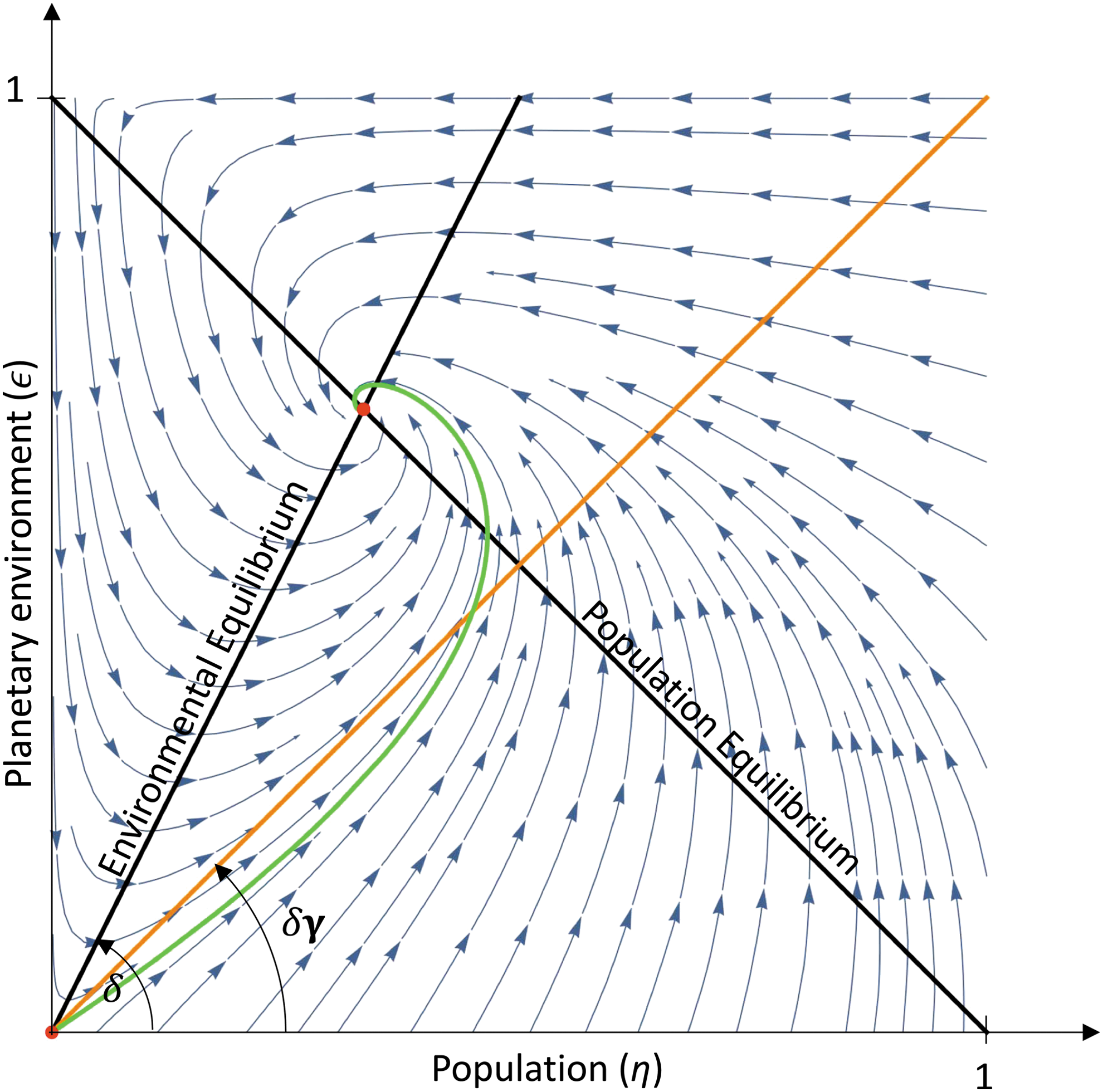
Schematic of a typical phase portrait. η is the nondimensional population, and ε is the nondimensional environmental state. The nullclines for population and environment are shown in black, and the equilibria are shown in red. The population nullcline goes from (0, 1) to (1, 0), while the environmental nullcline leaves the origin with slope δ. Note the saddle at the origin and the spiral sink. Also shown in orange is the tangent to the phase trajectory at the origin whose slope is given by γδ, as well as the trajectory from the origin to the stable equilibrium in green.
Consideration of the eigenvalues and eigenvectors of the Jacobian of the time derivatives given in Eqs. 10 and 11

shows the equilibrium at the origin to be a saddle point with eigenvalues {-γ, 1}, while the nontrivial equilibrium at
Since all the variables are strictly positive, the eigenvalues have a negative real component, and this solution is in general a sink. The behavior of solutions near the sink depends on the sign of the radicand in Eq. 16. When

Phase portrait for γ =
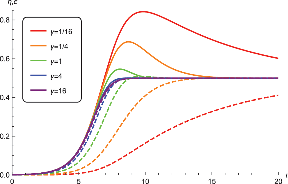
Time-series of population (η, solid line) and environment (ε, dashed line) for δ = 1 and various values for γ. Note that equilibrium for both population and environment for these parameters is at 1/2. When γ << 1, the population overshoots the equilibrium value and undergoes population decline, while for γ >> 1, the population reaches the equilibrium monotonically.
4.2. Parameter dependence
To understand the role of γ (the environmental sensitivity) and δ (the forcing), we consider the behavior of solutions starting near the origin shown by the green line in Fig. 1. In the limit of pristine environment (ε → 0) and very low population (η → 0) we have
Conceptually, for high sensitivity (γ >> 1), the environmental impact and recovery terms are fast, and the environment remains just below equilibrium as the population grows as shown in the right panel of Fig. 2. As the population reaches equilibrium, the environment is already at near equilibrium, so there is little or no overshoot in population. On the other hand, for low sensitivity (γ << 1), the environment is slow to respond, and the population reaches the carrying capacity for an environment well out of equilibrium as seen in the left panel of Fig. 2. This lag in the environmental response leads to a die-off as the carrying capacity decreases as the environment degrades on its way to equilibrium.
While γ determines how far from environmental equilibrium one gets, the forcing δ determines how low the eventual equilibrium population will be, since the equilibrium population will be η
* =
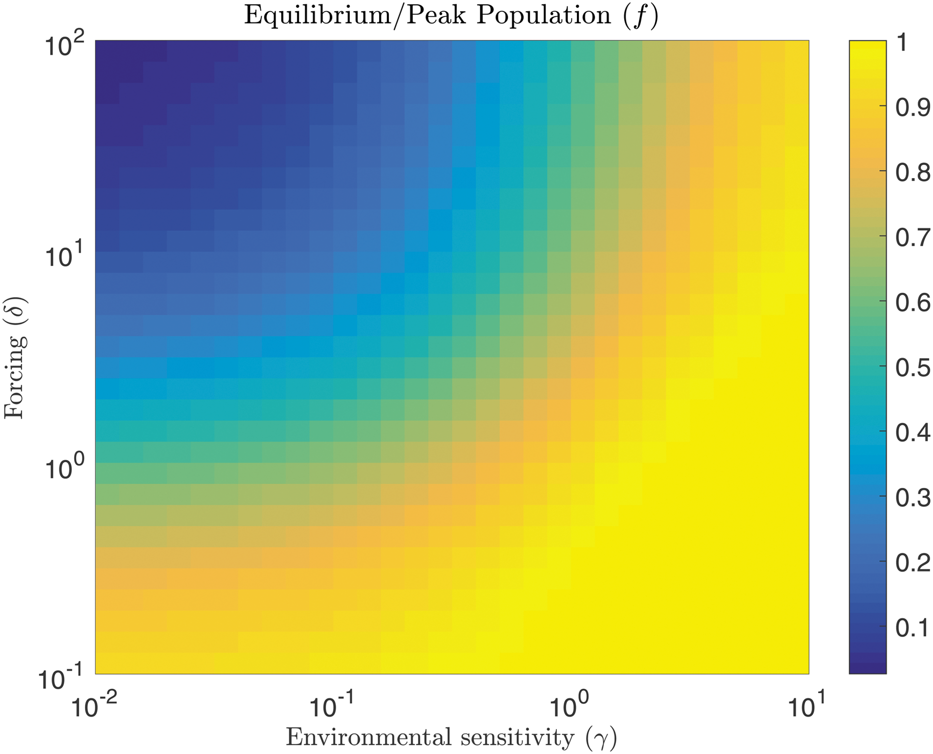
Ratio of equilibrium to peak population for various values of environmental sensitivity (γ) and forcing (δ). For large values of γ or small values of δ there is little to no die-off, while for small values of γ and large values of δ the population can be reduced to <10% of its peak.
5. Model 2: Interaction with Choice between Two Resources
Every resource used will have some degree of environmental impact. Thus we now extend the model by including a transition from use of a high-environmental-impact resource to one with a lower impact. For simplicity we consider the second resource to have no impact but keep the same consumption benefit. The transition occurs when the environment reaches some fraction of critical
This system reduces to
The equations above show the means for representing exo-civilization “sociology” via simple parameterization. Here the complex processes involved in an intelligent technological species recognizing its impact on the host planet's coupled systems and its subsequent moves to deal with those impacts are represented by two parameters. First, Φ represents the degree of departure from the initial planetary state at which the civilization initiates its switch in resource modalities. Thus we consider it to be a measure of the civilization's foresight. Note that low values of Φ correspond to switching resource modes earlier and represent higher degrees of foresight. Second, the term λ represents the speed at which that switch is enacted. Such a methodology can be extended as more details in the model interaction between an exo-civilization and its host planetary systems are included.
We note that in the current model when λ << 1 the behavior is unchanged for ε < Φ, while for ε > Φ the consumption detriment term is cancelled.
Figure 5 shows a typical solution for γ =
Phase portraits for two resource solutions where the transition time between the resources is varied. For the solution on the left, the transition is early enough to avoid risk of population decline (higher foresight). For the solution on the right, the transition is too late to avoid population die-off (lower foresight). The plots correspond to γ =

Time-series of population (η, solid line) and environment (ε, dashed line) for δ = 4, γ =
6. Model 3: Nonlinear Planetary Interaction (Runaway)
Our third model modifies the environmental self-regulation to include a nonlinear “heating” term which leads to runaway environmental degradation for ε >
For simplicity we first ignore the resource transition by dropping the
Figure 7 shows a typical phase diagram. There are two equilibria where the parabola for the environmental nullcline intersects the η = 0 axis at (0, 0) and at (0, 1/ξ). The trivial equilibrium at the origin is still a saddle with eigenvalues 1 and -γ, and the equilibrium at (0, 1/ξ) is an unstable node with eigenvalues 1 and γ. The other two equilibria can be written as

Schematic of a typical phase portrait when there is environmental instability and no resource transition. The nullclines for population and environmental equilibria are shown in black, and the stationary points are shown in red. The population nullcline goes from (0, 1) to (1, 0) while the environmental nullcline leaves the origin with slope δ and then bends back to the null point at (0, 1/ξ). Also shown in orange is the tangent to the phase trajectory at the origin whose slope is given by γδ, as well as the trajectory from the origin to the stable equilibrium in green.
where
The stability of the different equilibria depends on analysis of the parameters' regimes. We present that analysis in Appendix A noting here that the (ξ, δ) plane corresponding to the environment's fragility and the forcing separates the equilibria into distinct regions with different stability properties ranging from stable nodes to unstable foci shown in Figs. 8 and 9. We also note that a bifurcation occurs leading to limit cycles in the solutions.

Plot showing number and type of solutions for different values of δ and ξ for γ < 1.
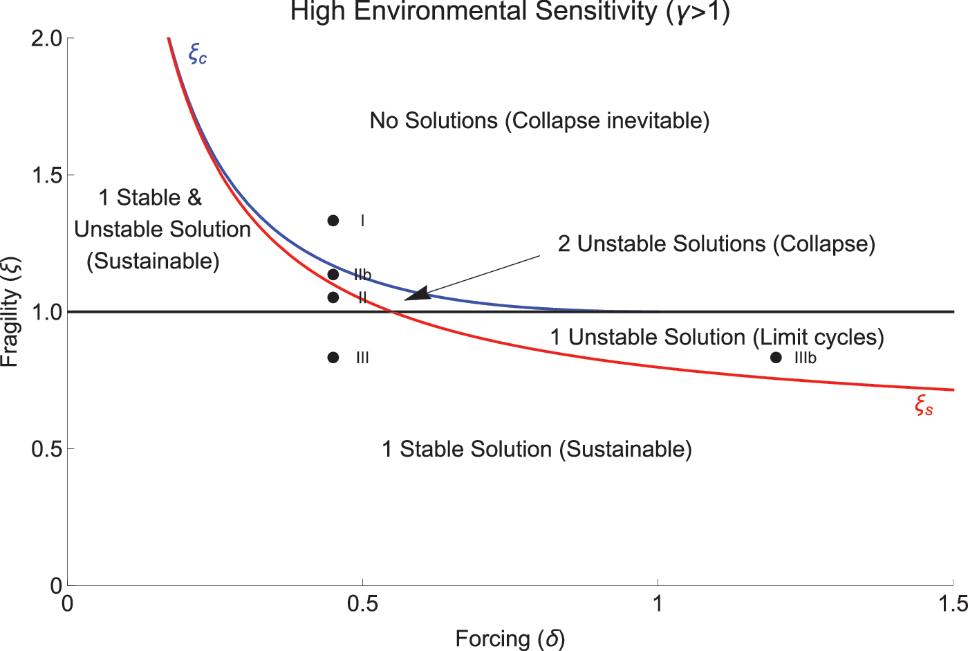
Plot showing number and type of solutions for different values of δ and ξ for γ > 1.
We can define two important regimes for the solutions based on parameters we now introduce: ξ
c is a critical fragility for equilibria to exist, and ξ
s is a critical fragility for those equilibria to be stable. In particular, when
6.1. Model 3 behavior: single resource
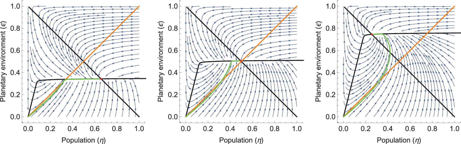
Figure 10 shows phase portraits for various parameter regimes, while Fig. 11 shows time-series for those solutions. We first note the rich behavior seen in those plots. Here we vary the environment's fragility ξ and the resource's environmental forcing δ in regimes where the environment is either slow (low sensitivity γ << 1) or quick (high sensitivity γ >> 1) in responding to changes in population.
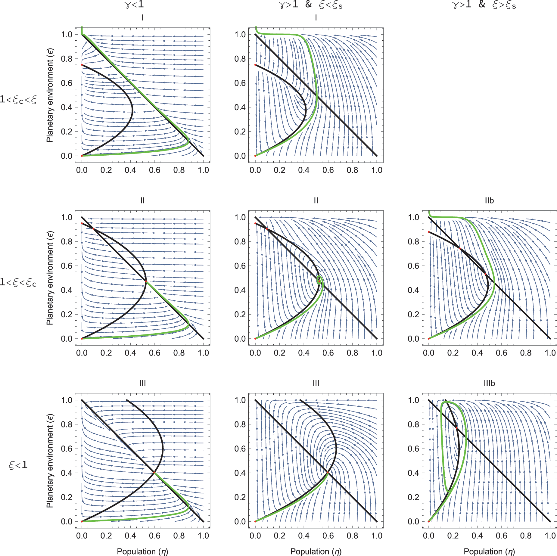
Phase portraits along with trajectories from the origin for the various solutions shown in Figs. 8 and 9. The left column shows the three solutions for γ = .1 (low planetary sensitivity), while the middle and right columns show the solutions for γ = 10 (high planetary environment sensitivity). In the top row, ξ > ξ c, and there are no physical solutions; and regardless of γ, extinction occurs. The second row shows solutions for 1 < ξ < ξ c. The upper solution is always a saddle, but the lower solution can be a stable focus for γ < 1 or for γ > 1 and ξ < ξ s, or it can be an unstable focus for γ > 1 and ξ > ξ s. The bottom row shows solutions for ξ < 1 where there is always just one solution that can also be a stable focus for γ < 1 or for γ > 1 and ξ < ξ s, or it can be an unstable focus for γ > 1 and ξ > ξ s. Note the existence of a limit cycle in the bottom right panel around the unstable focus, while in the middle row, the unstable focus does not produce a limit cycle.
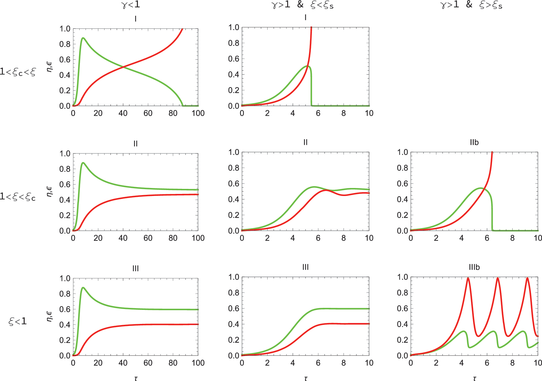
The left column of Fig. 10 shows the solutions for a slowly responding environment (γ = .1), while the middle and right columns show the solutions for a quickly responding environment (γ = 10). In the top row we have ξ > ξ c. Given the forcing in these cases, the environment is too fragile to yield an equilibrium solution with a sustained population. For these solutions, regardless of the value of γ, we see extinction occur as the population declines to η = 0. Consideration of the time-series in Fig. 11 shows the different timescales for extinction to occur. In the top left we see that population reaches its peak and then begins a slow decline to zero as the environment slowly responds to the increased population. In the top middle panel we see the population reach its peak and then quickly drop to zero due to a more rapid environmental runaway. This represents a collapse solution.
The second row of Fig. 10 shows solutions for 1 < ξ < ξ c in which case the parabola representing the environmental nullcline intersects the population nullcline at two points. The upper equilibrium is always an unstable saddle, but the lower solution can be a stable focus for slowly responding environments (γ < 1), or for quickly responding environments (γ > 1) provided the environment is not too fragile (ξ < ξ s). If γ > 1 and ξ > ξ s, the environmental response is too fast (or equivalently the population response is too slow) to avert disaster, and the solution becomes an unstable focus. The time-series in Fig. 11 shows that these solutions correspond to varying degrees of die-off (left middle and central panels) or collapse (right middle panel). Note also that in the central panel we see the beginning of oscillatory behavior.
The bottom row of Fig. 10 shows solutions for ξ < 1 where there is always just one solution that can be a stable focus for γ < 1 or for γ > 1 and ξ < ξ s. It can be an unstable focus for γ > 1 and ξ > ξ s. Note that unlike the case where ξ > 1, the unstable focus now gives rise to a limit cycle shown in the bottom right panel. The time-series in Fig. 11 shows that these solutions correspond to die-off (lower left panel), a smooth approach to sustainability (lower middle panel), or a limit cycle (lower right panel).
6.2. Model 3 behavior: two resources
We now add the switch between resources to Model 3 and consider the case when ξ > ξ c where the environment is too fragile given the initial forcing and there is no stable equilibrium without a resource transition. We note again that we include the possibility of a second resource to model the civilization's attempt to switch to an energy modality that has less impact on the planetary environment (i.e., the civilization is trying to save itself). The second resource introduces a second parabola which is superposed onto the environmental nullcline. The location of the peak of the second parabola now controls the behavior of the solutions. Figure 12 shows phase portraits for various parameter regimes, while Fig. 13 shows time-series for those solutions.

Phase portrait for two-resource model with environmental instability. All plots correspond to the parameter regime without equilibria in single-resource model (type I in Figs. 8 and 9). The addition of the second resource can create new equilibria and prevent collapse. Left column corresponds to a slowly responding environment (low sensitivity). Right column corresponds to rapidly responding environments. Top row corresponds to resource transition made relatively far from critical value of environment (high foresight). In the rows that follow, the transition is made closer to environment's critical value (progressively lower foresight). In terms of parameter values, (δ, ξ) = (1/2, 4/3), with γ = .1 (left column) and γ = 10 (right column) with a quick resource transition λ = .05 near environmental instability Φ ≈ 1/ξ. Thus the top, middle, and bottom rows correspond to varying degrees of foresight in terms of switching resources before reaching ε =

Time-series for two-resource model with environmental instability. Population η is shown in green and the environment ε in red. Left column corresponds to a slowly responding environment (low sensitivity). Right column corresponds to rapidly responding environments. Top row corresponds to resource transition made relatively far from critical value of environment (high foresight). In the rows that follow, the transition is made closer to environment's critical value (progressively lower foresight).
The left column in Figs. 12 and 13 corresponds to an insensitive, slowly responding environment (γ << 1), while the right column in Figs. 12 and 13 corresponds to a quickly responding environment (γ >> 1). In the top row, the resource transition is early enough (high foresight) to avoid collapse, while in the middle row, collapse is only avoided in the γ << 1 regime. For γ >> 1, the population is too far from equilibrium and does not respond fast enough to avoid collapse during the resource transition. And in the bottom row, the resource transition is too late (low foresight), and collapse is inevitable, though in the γ << 1 regime there is a long period of apparent stability as the population sits on the tipping point. This can be seen especially in the bottom left panel of Fig. 13.
Consideration of Figs. 12 and 13 shows that once again we can find a variety of solution types ranging from die-off to collapse. What is noteworthy for some solutions is the delay that occurs when the transition from the high-impact to low-impact resource occurs. In particular the transition can help lead to long-term sustainable trajectories after a relatively small die-off (top right panel), or it can only forestall the eventual collapse (middle right panel). This behavior illustrates that, in principle, our methodology can illustrate how attempts to make the switch between resource types can succeed or fail.
In more detailed and explicit models (explicit in terms of using more realistic planetary response functions) it should be possible to determine the parameter space density of successful strategies available to exo-civilizations when faced with their own versions of an Anthropocene.
7. Discussion and Conclusions
We have used the formalism of dynamical systems theory to explore a highly simplified model for the interaction of a resource-intensive technological species with its host planet. In particular we have developed a set of coupled ODEs for the population and for the environment where the latter term refers to the dynamical state of the coupled planetary systems (atmosphere, hydrosphere, cryosphere, etc.). Our models posit an environmentally dependent carrying capacity K(e) along with population benefits and environmental detriments accruing from resource use. We explore the possibility of switching between resources with different planetary impacts. We also explore the role of nonlinear feedbacks in the form of a term driving runaways in the planetary environment.
We find four distinct classes of trajectories in our models.
Sustainability: For these classes, stable equilibria (n *, e *) exist which can be approached monotonically. The population rises smoothly to a steady-state value. The planetary environment is monotonically perturbed from its initial value e 0 and reaches a new steady state that can support a large population.
Die-off: For these classes, stable equilibria (n *, e *) exist which cannot be approached monotonically. The population overshoots the environment's carrying capacity, reaches a peak, and is forced to decline as the environment reaches its new steady state.
Collapse: For these classes, stable equilibria with nonzero population do not exist. In these cases the population experiences a rapid decline after reaching its peak value. It is noteworthy that collapse can occur even though the population has begun leveling off due to the civilization's switching from high-impact to low-impact energy modalities.
Oscillation: In this class, a stable limit cycle exists rather than an equilibrium. The population and the planetary environment cycle between high and low values.
We first note that our study was specifically intended as a demonstration of the methodology. Our models are a highly simplified representation of the true complexity inherent in the interactions between a civilization (human or otherwise) and the host planetary systems. Thus the different classes of trajectories observed in the models represent an initial exploration of the richness to be expected as we begin building representations that capture higher degrees of veracity in the coupled dynamics of civilizations and their planetary system. What our study demonstrates is that it should be possible to capture essential elements of the interaction between planetary-systems dynamics and civilizations while also reducing the “sociological” aspects of the problem (i.e., agency in the form of decisions made by the species) to model input parameters.
By testing the proposed methodology, we intend to motivate the development of a research program that more realistically represents the planet-civilization interaction. This would include a more complete account of the role of planetary parameters such as orbital radii, atmospheric composition, incident stellar flux, and so on, in particular in terms of how these parameters affect resources needed by civilizations.
More complete models for resource impact would also need to be included. The number of resource modalities for a young civilization species is limited by physical considerations (for instance to energy resources such as biomass, fossil fuels, wind, hydrothermal, tidal, nuclear, etc.). Given a set of planetary and climate parameters, one can in principle calculate climate sensitivity for the use of each form of energy resource. For example, Miller et al. (2011) calculated climate sensitivity for the large-scale wind energy resource.
Solving the equations across the input parameter space volume for planetary system, population, energy modality choices and other agency-dependent parameters, a large ensemble of model civilization trajectories can be established. In this way we will have a trajectory bundle for our ensemble whose properties as a whole can be analyzed. The simplest question to ask of the bundle will be average lifetime of civilizations,
Such a program would be of interest to both astrobiological and Anthropocene studies. For example, as discussed in the introduction,
In addition to building more complete models of planet-civilization interactions, future studies will also have to include more complete consideration of the dynamical possibilities. We note the important role of “tipping points” in considering trajectories for the coevolution of coupled civilization-planet systems. A tipping point is a critical threshold where small perturbations can alter the large-scale state or evolution of a system. In mathematical terms, tipping points arise when bifurcations are seen in the behavior of system properties with respect to system parameters. Bifurcations can drive dynamical systems with slowly varying parameters into a transition to distant attractors.
Tipping points can be found through a variety of analysis methods including bifurcation theory. In the development of future models, particular attention should be paid to the ways in which the development of model equations for planet-civilization interaction will introduce tipping points into their dynamics. This will be particularly true as richer kinds of feedback between the planet and the civilization are added. In our current model, for example, the population's use of a resource only contributed negatively to the state of the resource. The development of sustainable civilizations may, however, include specific attempts to create/evolve cooperative relationships with the biosphere such that some interactions increase the availability of the resource, for example, by greening the desert to increase food production using technology (Kleidon, 2012). Including stochasticity to the models is another possible addition that should be considered to consider the possible effects of extreme events such as disease outbreaks or asteroid impacts.
We note that our models could be generally described as exploring the development material-limited chemoautotrophic/heterotrophic biospheric systems with the civilization being the primary agent for forcing on the other planetary systems. As civilizations begin to have stronger impacts on their planets, they will need to learn to power their activity in ways that lower global forcing. This may always be a material-limited process to some degree, since technologies are always physically instantiated. One can also argue that in switching between energy resources of different levels of forcing there may be a trajectory leading civilizations to an ultimate dependence on solar power. The history of photosynthetic life on Earth shows an interesting progression from one set of limiting resources for global photosynthesis (rare electron donors in the form of materials like iron ions) to an abundant electron donor (water). These evolutionary developments ultimately allowed for the colonization of the land by photosynthesizers. The development of technological civilization may prove to be continuing that trend via an eventual dependence on efficient conversion of solar photons to useful power via photovoltaics or other technologies. No energy modality is free from feedback, however, so relevant to these points, our models will need to explore how the coupled planetary-civilization system responds to transitions between energy modalities (including solar) given specific representations of planetary feedback processes (Frank et al., 2017).
Finally, we return to one of the principle astrobiological motivations for this study: the final factor (L) in Drake's equation. In this work we have developed a simple model for planet-civilization interactions. Our model includes a number of input parameters which, we have seen, control the trajectory of the development of the system (i.e., forcing, sensitivity, fragility, etc.). In principle, we could run the models over an ensemble of combinations of these inputs to create an ensemble of trajectories. This ensemble would yield distributions of key measures from which moments can be derived. In this way an average lifetime for civilizations could be defined and measured. Given the highly simplified nature of the models we present in this study, we have not carried forward such an exploration. Our work can, however, be seen as a first step in creating such average lifetimes which would represent a theoretical estimate of Drake's final factor. The next step would be including a more realistic climate model, empirically based estimates for different resources' forcing, and running the models over a variety of planetary conditions (orbital distance, stellar type, atmospheric composition, etc.). In this way our method would allow meaningful theoretical estimates of Drake's final factor to be calculated. This is a direction we intend to pursue in future work.
As discussed above, such theoretical estimates of L would be novel and would be of interest for studies in both astrobiology and the Anthropocene. Such work would, however, have important caveats. The lifetime so calculated would represent the ability of a civilization to navigate existential crises relevant only to sustainability. Factors such as aggression (nuclear conflict) or random events such as impacts or sterilization by local supernova or gamma-ray bursts would not be included. In addition, there may be other existential threats awaiting civilizations that make it through their versions of the Anthropocene, which cannot be included in our models. Still, given that humanity's current concern focuses exactly on issues of planetary feedback, our method for calculating L could provide some insight into the contours of our own choices and future.
In addition, values of L will be directly relevant to discussions of Fermi's paradox, as very low values could be seen as a solution to the question of “where are they” (the answer being “gone”). Thus if the development of Anthropocenes represents a fundamental bottleneck for civilizations' sustainability, it may be at least one filter that explains Fermi's paradox (Haqq-Misra and Baum, 2009).
The work initiated in this paper might provide connections to studies which aim to search for techno-signatures in exoplanets. A number of authors have begun to explore mechanisms by which civilizations may, through their activity, imprint detectable variations in exoplanet spectra. Proposals have come in the form of greenhouse gases (Lin et al., 2014), transits of artificial structures (Wright et al., 2016), or spectral signatures of such structures (large-scale deployment of surface photovoltaics [Lingam and Loeb, 2017]). The current work may have consequences in guiding the searches for such signatures. In addition, if such artifacts are discovered, they could serve as “input” parameters for the kinds of models we describe in this work.
To summarize, we have developed models of planet-civilization interactions that show that the onset of an Anthropocene-like transition may be a generic outcome of coevolution. Thus we might expect that on some subset of planets evolving exo-civilizations the host planetary system will be pushed out of the state in which the exo-civilization began. Our work opens up the possibility of a quantitative, theoretical Astrobiology of the Anthropocene. Future work can build on the current study by developing more realistic models of the planet-civilization interactions by including basic biogeophysical processes.
Appendix A. Characterization of Model 3 Equilibria Stability
Note for eigenvalues of solutions for Model 3 to be real, we must have a
2 - b > 0 or equivalently
The eigenvalues Γ1 and Γ2 at (η, ε)± are given by
where
At the other nontrivial solution (η, ε)+, since d > 0, the radicand of both eigenvalues will have less magnitude than (c - d), so the real component of both eigenvalues will have the same sign as (c - d). For c > d, the solution will be an unstable focus (or node); for c < d, it will be a stable focus (or node).
Now to have an unstable focus, we must have c > d or ξ
c > ξ > ξ
s
We also show in Fig. 10 the phase space and the evolution from the origin of each of the solutions shown in Figs. 8 and 9.