Abiotic and Biotic Formation of Amino Acids in the Enceladus Ocean

Abstract

The active plume at Enceladus' south pole makes the indirect sampling of its global ocean possible. The partially resolved chemistry of the plume, which points to conditions that are seemingly compatible with life, has made orbital sampling missions a priority. We present a conceptual model of energy flux, hydrothermal H₂ production, and both abiotic and biotic production of amino acids. Based on the energy flux observed at the south pole and the inferred internal hydrothermal activity, we estimate an H₂ production of 0.6–34 mol/s from serpentinization, sufficient to sustain abiotic and biotic amino acid synthesis of 1.6–87 and 1–44 g/s, respectively. Two-dimensional (2D) numerical simulations of the hydrothermal vent suggest that the vent fluids could reach the ice-water boundary in less than 11–55 days for a 50 km deep ocean diluted by ambient ocean water 10 to 1. Concentrations of glycine, alanine, α-amino isobutyric acid, and glutamic acid in the plume and in the ambient ocean could all be above 0.01 μM just due to abiotic production. Biological synthesis, if occurring, could produce a maximum of 90 μM concentrations of amino acids based on a methanogenic ecosystem consuming H₂ and CO₂. Racemization timescales in the ocean are short compared with production timescales. Thus, no enantiomeric excess is expected in the ambient ocean, and if biology is present, enantiomeric excess at the vent fluids is expected to be less than 10% in the plume. From vent H₂ concentrations of 7.8 mM (e.g., Lost City) and assuming complete H₂ use and conversion to chemical energy by methanogens, cell production is estimated. Annual biomass production in the methanogenic-based biology model is 4 × 10⁴–2 × 10⁶ kg/year. This corresponds to cell concentrations ∼10⁹ cells/cm³ in the vents and ∼10⁸ cells/cm³ in the plume, and when diluted into the ambient ocean, we predict cell concentrations of 80–4250 cells/cm³. Key Words: Abiotic organic synthesis—Enceladus—Extraterrestrial life. Astrobiology 17, 862–875.

1. Introduction

The discovery of Enceladus' plume of icy grains and gas by the Cassini mission (Porco et al., 2006; Waite et al., 2009; Postberg et al., 2011) has made this world an exciting target for further missions to the Saturn system. The plume contains salts, organic compounds, and silica nanoparticles, pointing to a subsurface, salty ocean in direct contact with a rocky core, and with ongoing hydrothermal activity (Waite et al., 2009; Postberg et al., 2011; Hsu et al., 2015; Sekine et al., 2015). The active plume emanates from four quasi-linear cracks in the moon's South Polar Terrain (SPT), where the majority of Enceladus' measured thermal flux occurs.

The discovery of volatile aliphatic hydrocarbons in the gas portion of the plume (Waite et al., 2009) and the inferred presence of refractory organics in icy particles, containing aromatic, long-chained, or polar hydrocarbons (e.g., alcohols, acids, nitriles, and amines) (Khawaja et al., 2015; Postberg et al., 2015), point to a certain degree of organic chemical evolution in the Enceladus ocean. In an attempt to further constrain the extent of organic chemical evolution in the system, we focused on possible pathways of amino acid synthesis.

We used the thermal flux observed at the SPT to estimate hydrogen (H₂) production by alkaline low-temperature hydrothermal activity at the ocean-sediment interface. The abiotic and biotic formation of amino acid was then modeled under these conditions, and the development of biomass and their concentrations were determined by the availability of chemical energy and nutrients entering the system. Ocean convection modeling was used to understand the transport of species from the ocean floor to the plumes and their dilution.

2. Materials and Methods

2.1. Thermal energy model

Observations of the SPT using the 10–600 cm⁻¹ spectrum of the Cassini Composite Infrared Spectrometer (CIRS) predict a total heat flux from Enceladus of 15.8 ± 3.1 GW (Howett et al., 2011). The measured heat flux far exceeds the combined energy output of the predicted current radiogenic (∼0.3 GW; Porco et al., 2006) and long-term tidal heating (∼1.1 GW; Meyer and Wisdom, 2007). Averaged over the active terrain below 65° S, the corresponding regional heat flux is ∼400 mW/m² (Bland et al., 2012). Here, it is assumed that the heat flux in the Enceladus ocean is equal to that measured at the surface. We note, however, that Enceladus may undergo periodic fluctuation in heat dissipation (O'Neill and Nimmo, 2010; Hansen et al., 2011), and the regional heat flux has likely changed through time (Bland et al., 2012).

Since the sources that are responsible for the observed heat flux over the SPT are unknown, and the coupling between the ocean and rocky core is unconstrained, three models were developed to estimate the thermal energy available at the ocean-core interface for hydrothermal activity. Each model represents a progressive increase in the heat flux from the core: (1) Model I is typical of a rocky core with radiogenic heating only (∼0.3 GW); (2) Model II is the same as Model I but includes tidal energy dissipation (∼1.1 GW); and (3) Model III is the high-energy end-member case that has a power output equal to that of the current ocean (∼16 GW). Model III assumes that the majority of current thermal flux observed in Enceladus originates from the core. In each case, the distribution of heat flow from the core into the ocean was assumed to occur though hydrothermal activity (34%) and diffusive heat flow (66%), based on the Earth's ocean floor; these figures are comparable to the (1 to 1) ratio assumed for Europa by Lowell and DuBose (2005). The activity and circulation of the global ocean in all three models were assumed to be driven by a convective ocean current focused under the SPT.

2.2. Hydrogen production model

Results from the heat flow models (Table 1) were used to estimate H₂ production by alkaline, low-temperature hydrothermal activity at the ocean-sediment interface. Other abiotic sources of H₂, such as thermal decomposition of alkanes and carboxylic acids and mechanoradical formation on wet fault surfaces (Lin et al., 2005; Hirose et al., 2011), were not considered in the absence of significant tectonic activity in Enceladus. Hydrogen production was calculated by using a simple heat balance (Eq. 1) that was applied to the model heat fluxes, and it was independently estimated by using a mean diffusion distance. The fracture model of Vance et al. (2007) was updated and used to identify the extent of possible serpentinization. Properties reflecting basal temperature were updated to reflect the recent work of Hsu et al. (2015). The throughput of hydrothermal fluids was quantified from a simple heat balance: \documentclass{aastex}\usepackage{amsbsy}\usepackage{amsfonts}\usepackage{amssymb}\usepackage{bm}\usepackage{mathrsfs}\usepackage{pifont}\usepackage{stmaryrd}\usepackage{textcomp}\usepackage{portland, xspace}\usepackage{amsmath, amsxtra}\usepackage{upgreek}\pagestyle{empty}\DeclareMathSizes{10}{9}{7}{6}\begin{document} \begin{align*} Q = { \frac { { H_ { \rm H } } } { { c_ { \rm w } } \Delta T } } \tag { 1 } \end{align*} \end{document}

Table 1.

Model Heat Flux

	Model I 0.3 GW	Model II 1.4 GW	Model III 16 GW
Total averaged flux (mW/m²)	0.72	3.4	38.4
Hydrothermal (mW/m²)	0.25	1.1	13.1
Diffusion (mW/m²)	0.48	2.2	25.4

The average flux is the power averaged over the surface area of the ocean-core interface. R _core = 182 km. The contribution from hydrothermal and diffusive sources is set analogous to the Earth (34% and 66%, respectively) (Stein and Stein, 1994).

where Q is the flux of hydrothermal fluids, ΔT is the temperature difference between ocean water and the core, H _H is the heat output of the specific model, and c _w is the specific heat of water. The temperature difference between ocean water and the core was taken as 90 K, with the lowest estimate by Hsu et al. (2015).

For the hydrothermally carried heat flow, a high-temperature portion (30%) ΔT = 90 K was assumed. The remaining hydrothermal heat (70%) is assumed to be transported by low-temperature flow ΔT = 10 K, where rock-water temperatures have not equalized. This is similar to terrestrial environments where the majority of advective cooling occurs at lower temperatures (Stein and Stein, 1994). Lowell and Dubose (2005) estimated the distribution of high- and low-temperature heat flow on Europa in a similar manner. H _H is the portion of heat transported by high-temperature hydrothermal flow and is taken to be ∼10% of total heat flux. A similar scheme was used by Lowell and Dubose (2005) for estimating the energy output of hydrothermal systems on Europa. Assuming H₂ concentrations to be similar to those of the Lost City vents, 7.8 mM (Konn et al., 2015), a global flux may be calculated.

2.2.1. Serpentinization reactions

We assumed the same peridotite composition used by Vance et al. (2007, 2016) in the modeling of Europa and other small ocean planets, and we used the hydration of forsterite as a measure of total serpentinization. To draw comparisons with these studies, we assumed the core to be olivine rich, similar to an Earth mantle-like composition, while recognizing that Enceladus' rocky core might be more similar to carbonaceous chondrites (Sekine et al., 2015). The hydration of this material to serpentinite produces the stable phases serpentine–((Mg,Fe)₃Si₂O₅(OH)₄), brucite–((Mg,Fe)(OH)₂), and magnetite–(Fe₃O₄). The overall process is moderated by the quartz-fayalite-magnetite buffer (Eq. 2) (Sleep et al., 2004, 2011). \documentclass{aastex}\usepackage{amsbsy}\usepackage{amsfonts}\usepackage{amssymb}\usepackage{bm}\usepackage{mathrsfs}\usepackage{pifont}\usepackage{stmaryrd}\usepackage{textcomp}\usepackage{portland, xspace}\usepackage{amsmath, amsxtra}\usepackage{upgreek}\pagestyle{empty}\DeclareMathSizes{10}{9}{7}{6}\begin{document} \begin{align*} 3{ \rm{F}}{{ \rm{e}}_2}{ \rm{Si}}{{ \rm{O}}_4} + 2{\rm H_2}{\rm O} \leftrightarrow 2{ \rm{F}}{{ \rm{e}}_3}{\rm O_4} + 3{ \rm{Si}}{{ \rm{O}}_2} \left( {{ \rm{aq}}} \right) + 2{\rm H_2} \tag{2} \end{align*} \end{document}

The heat of the reaction for the peridotite-serpentine conversion is ∼41 kJ/mol (Macdonald and Fyfe, 1985; Vance et al., 2007). Serpentinization may be controlled by the diffusion of water from a crack network into the host body. Macdonald and Fyfe (1985) described such a scenario where permeability is controlled by the propagation of episodic fracturing that occurs at an accumulation of stress. In this scenario, the mean diffusion distance, \documentclass{aastex}\usepackage{amsbsy}\usepackage{amsfonts}\usepackage{amssymb}\usepackage{bm}\usepackage{mathrsfs}\usepackage{pifont}\usepackage{stmaryrd}\usepackage{textcomp}\usepackage{portland, xspace}\usepackage{amsmath, amsxtra}\usepackage{upgreek}\pagestyle{empty}\DeclareMathSizes{10}{9}{7}{6}\begin{document}$$\left\langle z \right\rangle$$ \end{document} , (Eq. 3) was used as a benchmark for the progression of reactions. Because the infiltration of water is expected to be relatively homogenous laterally, an extension to the 2D solution would not be appropriate. A diffusion constant (D = 5 × 10⁻⁷ cm²/s) corresponding to a test temperature of 373 K was used (Macdonald and Fyfe, 1985). The progression of the serpentinizing front was used to estimate a volume of lazerite serpenitinized (Eq. 4) and H₂ production (Eq. 5). \documentclass{aastex}\usepackage{amsbsy}\usepackage{amsfonts}\usepackage{amssymb}\usepackage{bm}\usepackage{mathrsfs}\usepackage{pifont}\usepackage{stmaryrd}\usepackage{textcomp}\usepackage{portland, xspace}\usepackage{amsmath, amsxtra}\usepackage{upgreek}\pagestyle{empty}\DeclareMathSizes{10}{9}{7}{6}\begin{document} \begin{align*} \left\langle z \right\rangle = \sqrt {2Dt} \tag{3} \end{align*} \end{document} \documentclass{aastex}\usepackage{amsbsy}\usepackage{amsfonts}\usepackage{amssymb}\usepackage{bm}\usepackage{mathrsfs}\usepackage{pifont}\usepackage{stmaryrd}\usepackage{textcomp}\usepackage{portland, xspace}\usepackage{amsmath, amsxtra}\usepackage{upgreek}\pagestyle{empty}\DeclareMathSizes{10}{9}{7}{6}\begin{document} \begin{align*} V = \frac { 4 } { 3 } \pi \left( { { R^3 } - { { \left( { R - \left\langle z \right\rangle } \right) } ^3 } } \right) \tag { 4 } \end{align*} \end{document} \documentclass{aastex}\usepackage{amsbsy}\usepackage{amsfonts}\usepackage{amssymb}\usepackage{bm}\usepackage{mathrsfs}\usepackage{pifont}\usepackage{stmaryrd}\usepackage{textcomp}\usepackage{portland, xspace}\usepackage{amsmath, amsxtra}\usepackage{upgreek}\pagestyle{empty}\DeclareMathSizes{10}{9}{7}{6}\begin{document} \begin{align*}{N_{{\rm H_2}}} = V*f_{\rm s} \tag{5} \end{align*} \end{document}

where t is the time in seconds, R is the radius of Enceladus' core, V is the serpentinization volume, N _H2 is the moles of hydrogen produced, and f _s is the volume to molar conversion factor. The molar volume of olivine was taken as representative of lherzolite (V _Lhe), which is 43.79 cm³/mol (Macdonald and Fyfe, 1985). Mean diffusion distance over 1 million years (Myr), averaged for a yearly rate, was calculated. By using the composition of lherzolite and noting the ratio of fayalite to H₂ (Eq. 2), a conversion factor f _s (1.06 × 10³ mol/m³) was used to convert a yearly volume of serpentinization to H₂ production (Eq. 5). This conversion factor falls between those used by Vance et al. (2007) (1 × 10³ mol/m³) and Sherwood Lollar et al. (2007) (1.4 ×10⁻³ mol/m³).

2.2.2. Fracturing

We modeled micro-fracturing from the thermal expansion/contraction of mineral grains in partially serpentinized peridotite, to take into account availability of fresh material, which is essential to estimating H₂ generation from water-rock interactions. Thermal expansion anisotropies of silicate grains produce an average stress <σ> along grain boundaries described by the differential equation of Evans and Clarke (1980): \documentclass{aastex}\usepackage{amsbsy}\usepackage{amsfonts}\usepackage{amssymb}\usepackage{bm}\usepackage{mathrsfs}\usepackage{pifont}\usepackage{stmaryrd}\usepackage{textcomp}\usepackage{portland, xspace}\usepackage{amsmath, amsxtra}\usepackage{upgreek}\pagestyle{empty}\DeclareMathSizes{10}{9}{7}{6}\begin{document} \begin{align*}{{d \left\langle \sigma \right\rangle } \over {{ \rm{dT}}}} = {{ \rm{96}} \Omega { \delta _{\rm D}{D_0}E} \over { \sqrt 3 { \rm{k}}{{ \rm{d}}^3}{{dT} \over {dt}}}}{{{e^{{{ - Q} \over {{ \rm{RT}}}}}}} \over T} \left\langle \sigma \right\rangle - {{{ \rm{ \beta {\it E} \Delta \alpha }}} \over {1{ \rm{ + \gamma }}}} \tag{6} \end{align*} \end{document}

The accumulation of stress occurs below the threshold temperature T′, defined as the solution to \documentclass{aastex}\usepackage{amsbsy}\usepackage{amsfonts}\usepackage{amssymb}\usepackage{bm}\usepackage{mathrsfs}\usepackage{pifont}\usepackage{stmaryrd}\usepackage{textcomp}\usepackage{portland, xspace}\usepackage{amsmath, amsxtra}\usepackage{upgreek}\pagestyle{empty}\DeclareMathSizes{10}{9}{7}{6}\begin{document}$$\left\langle { \sigma ( T{\prime} ) } \right\rangle = 0$$ \end{document} . To avoid the need for numerical methods in solving (6), the series approximation (7) was used for the calculation of T′. \documentclass{aastex}\usepackage{amsbsy}\usepackage{amsfonts}\usepackage{amssymb}\usepackage{bm}\usepackage{mathrsfs}\usepackage{pifont}\usepackage{stmaryrd}\usepackage{textcomp}\usepackage{portland, xspace}\usepackage{amsmath, amsxtra}\usepackage{upgreek}\pagestyle{empty}\DeclareMathSizes{10}{9}{7}{6}\begin{document} \begin{align*} T { \prime } \approx \frac { \frac{Q} {R_g} } { { \rm { ln } } \left[ { { \frac { { \rm { 96 } } \Omega { \delta _D } { D_0 } E } { \sqrt 3 { \rm { nk } } { { \rm { d } } ^3 } { \frac { dT } { dt } } } } } \right] } \tag {7} \end{align*} \end{document}

Fractures develop along grain boundaries where the stress (K _I) exceeds a critical toughness (K _IC). The stress normal to a grain boundary—σ_yy(x,T, T′)—with flaw size (x) and grain diameter (d) was modeled as: \documentclass{aastex}\usepackage{amsbsy}\usepackage{amsfonts}\usepackage{amssymb}\usepackage{bm}\usepackage{mathrsfs}\usepackage{pifont}\usepackage{stmaryrd}\usepackage{textcomp}\usepackage{portland, xspace}\usepackage{amsmath, amsxtra}\usepackage{upgreek}\pagestyle{empty}\DeclareMathSizes{10}{9}{7}{6}\begin{document} \begin{align*} \begin{split} { \sigma _ { { \rm { yy } } } } \left( { { { x , T , T { \prime } } } } \right) = { \frac { { \rm { \it E } { \Delta \alpha } } \left( { { { T { \prime } } } - T } \right) } { 2 \pi \left( { 1 - { \gamma ^2 } } \right) } } \left( { { \frac { { d^2 } } { { d^2 } + { { \left( { d - x } \right) } ^2 } } } } \right.\\\left.\quad- { \frac { { d^2 } } { { d^2 } { \rm { + } } { { \rm { x } } ^2 } } } + { \rm { ln } } \left[ { \frac { { d - x } } { x } } \right] - \frac { 1 } { 2 } { \rm { ln } } \left[ { { \frac { { d^2 } + { { \left( { d - x } \right) } ^2 } } { { d^2 } { \rm { + } } { { \rm { x } } ^2 } } } } \right] \right) \end{split}\tag { 8 } \end{align*} \end{document}

Stress intensity is a function of the normal stress, confining pressure P _c and flaw size. The presence of a thermal state that is significantly lower than the material's “freezing” temperature T′ and the absence of a sufficient confining pressure will promote fracturing where K _I exceeds K _IC. \documentclass{aastex}\usepackage{amsbsy}\usepackage{amsfonts}\usepackage{amssymb}\usepackage{bm}\usepackage{mathrsfs}\usepackage{pifont}\usepackage{stmaryrd}\usepackage{textcomp}\usepackage{portland, xspace}\usepackage{amsmath, amsxtra}\usepackage{upgreek}\pagestyle{empty}\DeclareMathSizes{10}{9}{7}{6}\begin{document} \begin{align*} K_{\rm I} = \sqrt {{2 \over {{ \rm{ \pi \it a}}}}} \mathop {\int \limits_0^a} {{{ \sigma _{{ \rm{yy}}}} \left( {{{ x , T , T \prime}}} \right) \sqrt x } \over { \sqrt { \left( {a - x} \right) } }}{ \rm{dx}} - P_{\rm c} \sqrt { \left( {{ \rm{ \pi \it a}}} \right) } \tag{9} \end{align*} \end{document}

Descriptions and values of all aforementioned parameters are listed in Table 2. The flaw size, a, was allowed to extend from the grain boundary (x = 0) to a distance a < d. Where appropriate, the values of parameters were conservatively selected to minimize calculated fracture depth, representing a low-end scenario for available serpentinizing regions and H₂ production. Values of critical fracture toughness (K _IC) of olivine in hydrothermal areas ranging from 0.65 to 2 MPa m^1/2 have been proposed (Demartin et al., 2002; Balme et al., 2004); the upper limit was selected for the model. The flaw size that maximizes K _I was selected from Figure 1 and tabulated for various temperatures. Equation 9 was equated with fracture toughness (K _IC) and solved for P _c at various temperatures to determine conditions at the cracking front.

FIG. 1.

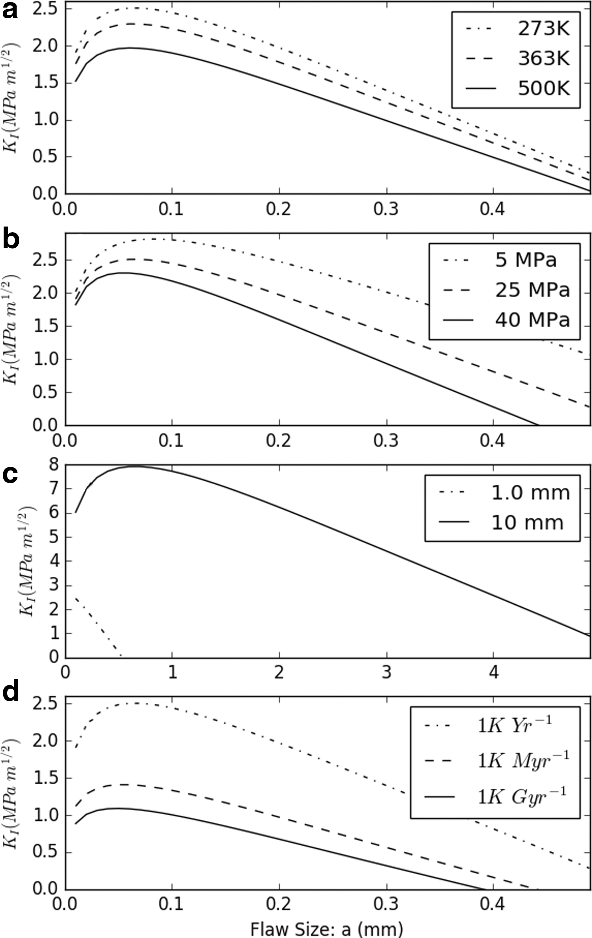
Stress intensity as a function of flaw size. Unless varied d = 1 mm, P_c = 25 Mpa, T = 273 K, T′ = 1 K/year. (a) Effect of temperature, (b) confining pressure, (c) grain size, and (d) cooling rate on stress intensity.

Table 2.

Physical Properties of Enceladus Model

Parameter	Description	Units	Value	Reference
Ω	Atomic volume	m³	1.23 × 10⁻²⁹	Hirth and Kohlstedt (1995)
δ_D D ₀	Grain boundary	m²/s²	1.5 × 10^−0.8	Hirth and Kohlstedt (1995)
E	Young's Modulus	Pa	1.97 × 10¹¹	Vance et al. (2007)
β	Boundary angle	radians	π/6	Vance et al. (2007)
Δα	Thermal expansion anisotropy	K⁻¹	3.1 × 10⁻⁶	Bouhifd et al. (1996)
γ	Poisson's ratio		0.246
Q	Activation enthalpy	J/mol	3.15 × 10⁵	Hirth and Kohlstedt (1995)
R	Radius (core)	m	182 × 10³	Čadek et al. (2016)
z	Thickness of ocean/ice	m	70 × 10³
R _g	Universal gas constant	J/(mol kg)	8.314
k	Boltzmann's constant	J/K	1.38 × 10⁻²³
n	Fitting parameter		23	Vance et al. (2007)
d	Grain size	m
K _I	Stress intensity	Pa m^1/2
K _IC	Critical stress intensity	Pa m^1/2	0.75 × 10⁶	Demartin et al. (2002)
P _c	Confining pressure	Pa
a,x	Flaw size	m
T′	Threshold temperature	K
\documentclass{aastex}\usepackage{amsbsy}\usepackage{amsfonts}\usepackage{amssymb}\usepackage{bm}\usepackage{mathrsfs}\usepackage{pifont}\usepackage{stmaryrd}\usepackage{textcomp}\usepackage{portland, xspace}\usepackage{amsmath, amsxtra}\usepackage{upgreek}\pagestyle{empty}\DeclareMathSizes{10}{9}{7}{6}\begin{document}$$ { \frac { dT } { \rm dt } } $$ \end{document}	Cooling rate	K/s
\documentclass{aastex}\usepackage{amsbsy}\usepackage{amsfonts}\usepackage{amssymb}\usepackage{bm}\usepackage{mathrsfs}\usepackage{pifont}\usepackage{stmaryrd}\usepackage{textcomp}\usepackage{portland, xspace}\usepackage{amsmath, amsxtra}\usepackage{upgreek}\pagestyle{empty}\DeclareMathSizes{10}{9}{7}{6}\begin{document}$$ \rho _{\rm o}$$ \end{document}	Ocean density	kg/m³	1030	Čadek et al. (2016)
\documentclass{aastex}\usepackage{amsbsy}\usepackage{amsfonts}\usepackage{amssymb}\usepackage{bm}\usepackage{mathrsfs}\usepackage{pifont}\usepackage{stmaryrd}\usepackage{textcomp}\usepackage{portland, xspace}\usepackage{amsmath, amsxtra}\usepackage{upgreek}\pagestyle{empty}\DeclareMathSizes{10}{9}{7}{6}\begin{document}$$ \rho _{\rm c}$$ \end{document}	Core density	kg/m³	2400	Iess et al. (2014)

Neveu et al. (2015) concluded that the temperature and pressure dependence of E and γ are negligible in the ranges considered here; they are treated as constant.

Geotherms for Enceladus were calculated for each heat flux model (Section 2.1). A pressure gradient was calculated for a two-layered body by using values in Table 2. The geotherms are representative of a maximum temperature-worst case scenario and do not account for temperature dependences in thermal conductivity that can be significant (Clauser and Huenges, 1995).

2.3. Abiotic production of amino acids

Estimates of vent fluid flux at the ocean-core interface (Table 3) were used to calculate the expected net production of glycine (Gly) (Eq. 10) from abiotic hydrothermal reactions. Gly was chosen because it is the dominant species produced in abiotic serpentinizing experiments at lower (<373 K) temperatures (Islam et al., 2002; Higgs and Pudritz, 2009; Bassez et al., 2012; Kebukawa et al., 2017). A concentration of Gly in the vent fluid of 12.5 μM was used based on a scaled production value from experimental hydrothermal reactions in the presence of formaldehyde (Kebukawa et al., 2017). The initial concentration of formaldehyde in the work of Kebukawa et al. (2017) was ∼20 times that measured by Waite et al. (2009) in the plume. Assuming the plume concentration was representative of the bulk ocean, the Gly production at 90°C (249 μM) from the work of Kebukawa et al. (2017) was suitably reduced. This Gly concentration was scaled by its chondritic abundance (12%) to derive a total production value for the set of amino acids modeled.

Table 3.

Molecular Hydrogen Production

	Model I	Model II	Model III
Based on Heat Balance
H _H (GW) (30% of H _hydro)	0.03	0.14	1.63
Q (kg/s)	81	379	4332
H₂ (mol/s)	0.63	2.95	33.8
Based on Diffusion
Fracture Propagation (mm/yr)		0.0008
Volume of Serpentinization (m³/yr)		3.3 × 10⁵
H₂ (mol/s)		11 mol/s

Hydrothermal flow rate calculated for Models I, II, and III using a heat balance. Hydrogen production rate calculated from fluid diffusion induced cracking rate.

Other amino acid abundances were scaled according to relative abundances observed in the Murchison meteorite, which was considered an abiotic model mixture in thermodynamic equilibrium (Table 4). Two end-member scenarios were used as initial conditions to which abiotic amino acid production (Table 5) was added: (1) An ocean free of amino acids and (2) an ocean with an initial amino acid abundance equivalent to that observed in carbonaceous chondrites (i.e., Murchison) of 12 ppm (∼155 μM). \documentclass{aastex}\usepackage{amsbsy}\usepackage{amsfonts}\usepackage{amssymb}\usepackage{bm}\usepackage{mathrsfs}\usepackage{pifont}\usepackage{stmaryrd}\usepackage{textcomp}\usepackage{portland, xspace}\usepackage{amsmath, amsxtra}\usepackage{upgreek}\pagestyle{empty}\DeclareMathSizes{10}{9}{7}{6}\begin{document} \begin{align*}{\rm 2CO}_{2 \left( {aq} \right) } + NH_4^{ + 1} + 3{H_{2 \left( {aq} \right) }} \rightarrow glycin{e_{ \left( {aq} \right) }} + {H^{ + 1}} + 2{H_2}O \tag{10} \end{align*} \end{document}

Table 4.

Amino Acid Abundances Used in the Abiotic and Biotic Models

	Amino acid	Abundance (ppb) (% of total amino acids) Murchison (Glavin et al., 2010)	Abundance relative to Gly	Enantiomeric ratio (D/L) (Glavin et al., 2010)		Amino Acid	Aquatic relative abundance (%) (Moura et al., 2013)	Abundance relative to Gly
Abiotic	Glutamic (Glu)	1322 (6)	0.51	0.61	Biotic	Glutamic (Glu)	6.29	0.88
	Aspartic (Asp)	470 (2)	0.18	0.67		Aspartic (Asp)	5.39	0.75
	α-Alanine (Ala)	1310 (6)	0.50	0.82		Alanine (Ala)	8.95	1.25
	β-Alanine (Ala)	1081 (5)	0.41	0.82		Serine (Ser)	6.19	0.87
	Glycine (Gly)	2606 (12)	1	—		Glycine (Gly)	7.14	1
	AIB	5124 (24)	1.97	—
	Total	11913 (57)		—		Total	33.96

Amino acids selected represent the most abundant of those species identified in bulk samples. The d,l-enantiomers have been combined from the data of Glavin et al. (2010). Original data contain significant uncertainties that are not included here. Maximum enantiomeric excess (ee) is ∼20%. Abundances are given in parts per billion.

AIB, α-amino isobutyric acid.

Table 5.

Abiotic Amino Acid Concentrations in Hydrothermal Fluids Are Converted to a Total Production Using the Flow Rates in Table 3

	Model I	Model II	Model III
Vent amino acid concentration	103.75 μM
Amino acid production (mmol/s)	8.4	39.3	449.4

2.4. Biotic production of amino acids

The biotic production of amino acids was modeled while assuming synthesis rates by methanogens in alkaline hydrothermal vents. This approach has been used elsewhere for evaluating the potential of Mars and Europa to host a biosphere (Jakosky and Shock, 1998; McCollom, 1999), and it assumes a Gibbs free energy available from the reduction of CO₂ to CH₄ ∼125 kJ/mol. From the H₂ concentration estimated in the hydrothermal fluids (Section 3.2), this corresponds to 0.24 kJ/kg of flow. We used the energy requirement estimates of McCollom and Amend (2005) for the synthesis of biomass. For anoxic environments, ∼14 kJ/g was deemed appropriate; of this assembled biomass, amino acids represent about 60% (dry weight). The concentration of amino acids is given at 5160 μmol/g (McCollom and Amend, 2005). The relative abundance of amino acids in aquatic ecosystems on Earth (Moura et al., 2013) was used to derive the relative amino acid abundance resulting from biotic synthesis on Enceladus. To validate the results, adenosine triphosphate (ATP) production was used as a measure of biomass formation, by using the same initial H₂ concentration. It was assumed that ATP synthesis required 10 kcal/mol (Thauer et al., 1977), and 20 mmol of ATP was required for 1 g of cells (Decker et al., 1970).

2.5. Enantiomeric excess in amino acids

Enantiomeric excess (ee = (L − D)/(L + D)), where L and D are the concentrations of the levorotatory and dextrorotatory isomers, respectively, was estimated for Ala, Glu, and Asp in both the abiotic and biotic source models. An initial ee of 20% was assumed as a conservative case for the abiotic-source model, based on enantiomeric enrichment observed in meteoritic amino acids (Cronin and Pizzarello, 1997; Pizzarello et al., 2006, 2012; Glavin et al., 2012; Pizzarello and Yarnes, 2016). An ee of 100% was assumed for biotic amino acids synthesized de novo. Racemization rates at 273K, 298K, and 323K were used to constrain the amount of time that it would take for the amino acid mixture in the ocean to completely racemize.

The D/L abundance at time t (s) was estimated with (Eq. 14), where Q = (1 + D/L)/(1 − D/L) (Cohen and Chyba, 2000). Increasing temperatures have significant effects on the rate of racemization; a small increase can decrease the time taken by many orders of magnitude. The rate constant (k _ala) of Ala in solution is given by Eq. 11, Asp (Eq. 12), and Glu (Eq. 13); T is the temperature in Kelvin. \documentclass{aastex}\usepackage{amsbsy}\usepackage{amsfonts}\usepackage{amssymb}\usepackage{bm}\usepackage{mathrsfs}\usepackage{pifont}\usepackage{stmaryrd}\usepackage{textcomp}\usepackage{portland, xspace}\usepackage{amsmath, amsxtra}\usepackage{upgreek}\pagestyle{empty}\DeclareMathSizes{10}{9}{7}{6}\begin{document} \begin{align*}{ k_ { \rm ala } } = { e^ { 24.91 - \frac { { 15863 } } { T } } } \tag { 11 } \end{align*} \end{document} \documentclass{aastex}\usepackage{amsbsy}\usepackage{amsfonts}\usepackage{amssymb}\usepackage{bm}\usepackage{mathrsfs}\usepackage{pifont}\usepackage{stmaryrd}\usepackage{textcomp}\usepackage{portland, xspace}\usepackage{amsmath, amsxtra}\usepackage{upgreek}\pagestyle{empty}\DeclareMathSizes{10}{9}{7}{6}\begin{document} \begin{align*}{ k_ { \rm asp } } = { e^ { 23.34 - \frac { { 14725 } } { T } } } \tag { 12 } \end{align*} \end{document} \documentclass{aastex}\usepackage{amsbsy}\usepackage{amsfonts}\usepackage{amssymb}\usepackage{bm}\usepackage{mathrsfs}\usepackage{pifont}\usepackage{stmaryrd}\usepackage{textcomp}\usepackage{portland, xspace}\usepackage{amsmath, amsxtra}\usepackage{upgreek}\pagestyle{empty}\DeclareMathSizes{10}{9}{7}{6}\begin{document} \begin{align*}{ k_ { \rm glu } } = { e^ { 22.56 - \frac { { 15675 } } { T } } } \tag { 13 } \end{align*} \end{document} \documentclass{aastex}\usepackage{amsbsy}\usepackage{amsfonts}\usepackage{amssymb}\usepackage{bm}\usepackage{mathrsfs}\usepackage{pifont}\usepackage{stmaryrd}\usepackage{textcomp}\usepackage{portland, xspace}\usepackage{amsmath, amsxtra}\usepackage{upgreek}\pagestyle{empty}\DeclareMathSizes{10}{9}{7}{6}\begin{document} \begin{align*}{ \left( { \frac { D } { L } } \right) _t } = { \frac { Q { e^ { 2 { k_ { \rm ala } } t } } - 1 } { Q { e^ { 2 { k_ { \rm ala } } t } } + 1 } } \tag { 14 } \end{align*} \end{document}

2.6. Long-term average concentrations of amino acids

The thermal decomposition of amino acids in Enceladus' core was assumed to be the main loss term for amino acids in the ocean, in both the abiotic and biotic models. At temperatures >200°C, amino acids break down to their constituents; depending on the specific amino acid, this threshold temperature may vary (Yablokov et al., 2013). With the presence of mineral catalysts, the rate of decomposition is relatively rapid and the temperature required is reduced (McCollom, 2013). We assumed that amino acids decomposed in the core but remained unaffected in the cooler bulk ocean. To calculate long-term, average concentrations of free amino acids, a 1 kyr mixing time for the ocean was assumed, a value that was comparable to mixing times for the Earth's oceans (∼600 years; Toggweiler and Robert). Changes in species concentrations were derived after each model time step while taking into account the recycling of amino acids due to the ocean circulation into Enceladus' core.

2.7. Ocean convection and mixing model

MITgcm (Adcroft et al., 2004) is a general oceanic and atmospheric numerical model that is designed to run efficient geophysical fluid circulation problems. The model is highly customizable and is capable of handling non-hydrostatic fluid flow problems in 2D or three dimensions. The Enceladus model implemented herein was assumed to be axisymmetric, making a 2D domain a viable representation. The general physical and control parameters used were the same as those outlined by Goodman and Lenferink (2012) for Europa unless body specific; here, they have been updated for Enceladus accordingly. The parameter for Coriolis force corresponds to a plume on the South Pole, a latitude of 90°. The model was implemented over a 100 × 100 regular grid with spacing of 500 or 250 m; this corresponds to a 25–50 km deep ocean. Circulation driven by heating from below was simulated in this calculation by imposing a reduction in density (heat loss) at the top of the column. The density reduction was distributed over three cells at the center of the x axis such that flux for the two simulations corresponds to the entirety of the heat flow assumed for Models II and III: 1.4 and 16 GW, respectively. To estimate mixing during fluid ascent, we used MITgcm's salinity variable as a convenient passive tracer. A salt flux of 1 g/(m²·s) was set along the same three cells as the heat flux. The concentration at the ice shell was then a direct indicator of intervening mixing.

3. Results

3.1. Thermal energy

The distribution of heat flow at the ocean-sediment interface is presented in Table 1 for each Model scenario. The estimated total averaged heat flux over the surface area of the ocean-sediment interface ranged between 0.72 and 38.4 mW/m². Energy transported through high-temperature hydrothermal flow ranged between 0.25 and 13.1 mW/m². The latent heat stored within the Enceladus ocean was calculated from its volume. The average physical dimensions of the core and ice shell as determined by Čadek et al. (2016), an ocean depth of 50 km and a core radius of 182 km, give an ocean volume of ∼2.7 × 10¹⁶ m³.

3.2. Chemical energy

The fracturing model suggests that cracking would extend throughout Enceladus' rocky core. The variable cooling rates and limited grain sizes had the greatest effect on the calculated stress intensity (Fig. 1). Even for unrealistically low cooling rates (1 K/Gyr), the entirety of Enceladus' core was fractured (Fig. 2). The same fracturing model, assuming a cooling rate of 1 K/year, predicted a fracture depth of 5–6 km for the Earth, comparable to measurements from seismic surveys (Vance et al., 2007).

FIG. 2.

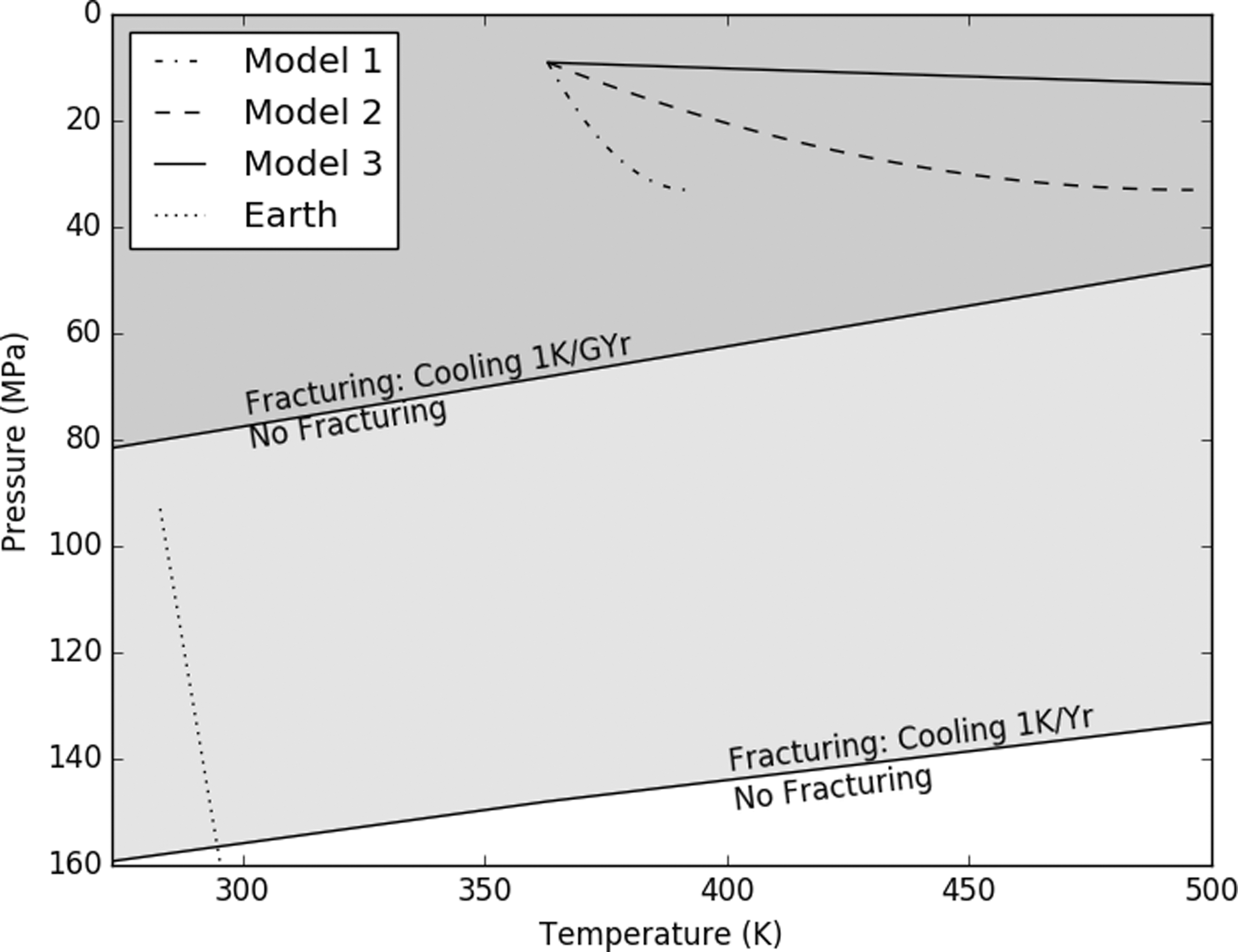
Fracturing fronts for different cooling rates. The pressure-temperature profiles for each Enceladus model are above the most conservative fracture front; micro-fracturing throughout the entire core may occur.

For the heat balance model, estimated rates of H₂ production ranged between 0.63 and 33.8 mol/s (Table 3). When the diffusion approach was considered, the net H₂ production rate was ∼11 mol/s over a shell that represents the serpentinization front at t = 4.6 Gyr. The estimated release of H₂ from olivine (0.047 mol_H2/mol_olv) compared favorably with experimental results of 0.044 mol_H2/mol_olv (Malvoisin et al., 2012). We note, however, that over geological periods, as the serpentinization front moves deeper into Enceladus' rocky core, the production area and the hydrogen flux calculated from it would decrease. H₂ production rates from the heat balance model, constrained by the measurable heat flux, were used to calculate abiotic and biotic amino acid production.

3.3. Abiotic source of amino acids

Amino acid production rates in hydrothermal reactions at the ocean-core interface ranged between 8.4 and 449.4 mmol/s, depending on the assumed heat balance (Table 5). For an initial free amino acid concentration in the ocean equivalent to that reported for the Murchison meteorite (155 μM), the initial concentration was slightly higher than the production value, and the amino acid concentration tended to decrease over time until a steady-state value of 103.8 μM was reached.

3.4. Biotic source of amino acids

The estimated net biotic production of amino acids by a putative methanogenic community (Fig. 3) in hydrothermal vents was 17 mg/kg of vent fluid flow, with a total amino acid concentration of 90 μM in the vent fluid. The estimated ATP production was ∼30 mg/kg for the same hydrogen flux. Considering thermal amino acid recycling due to ocean circulation through the core, the long-term average biotic amino acid concentrations in the ocean ranged between 4.8 μM (Asp) and 8.1 μM (Ala) for the species modeled. Racemization rates are shown in Figure 4 and total concentrations are shown in Figure 5.

FIG. 3.

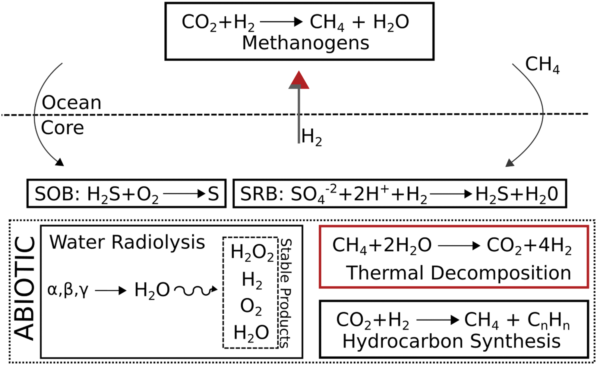
Summary of abiotic and biotic processes and their location in Enceladus. SOB = sulfide-oxidizing bacteria; SRB = sulfate-reducing bacteria.

FIG. 4.

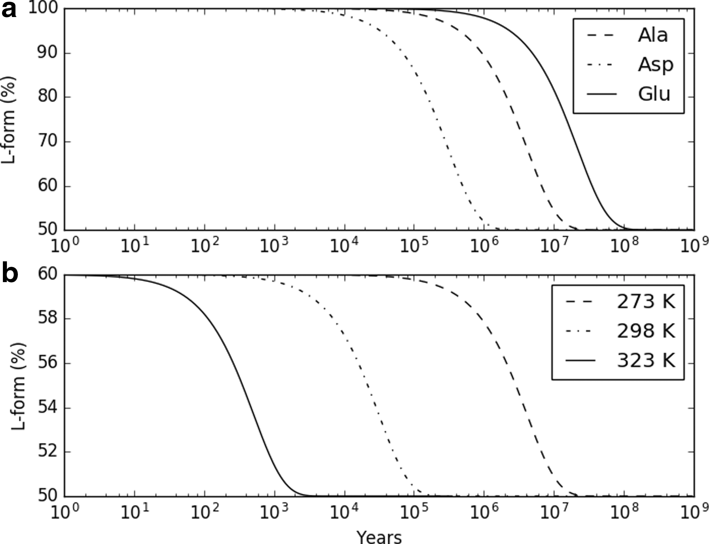
Racemization of aqueous amino acids. (a) Glu, Ala, and Asp with initial L-form concentration representative of biotic origins (b) Initial L-form excess for abiotic model, temperature dependence of alanine racemization.

FIG. 5.

Concentrations and chirality of selected amino acids in abiotic and biotic models as a function of time; production rate used is that of Model III. Top: Initial ocean concentration of zero. Middle: Percentage of L-enantiomer starting with an initial ocean concentration of zero. Bottom: Starting ocean concentration set to a chondritic analogue.

We calculated an annual biomass production of 4 × 10⁴–2 × 10⁶ kg/year. By comparison, the global carbon uptake by the terrestrial biosphere is 10¹⁴ kg/year (Field et al., 1998). Chyba and Phillips (2001) calculated the concentration of cells in an energy-limited europan ocean of 0.1–1 cells/cm³ with cells of mass 2 × 10⁻¹⁴ g. Assuming a similar 1 kyr period of cell destruction, we derived concentrations of 80–4250 cells/cm³ in the ocean and 8.5 × 10⁸ cells/cm³ in the venting fluids. Estimated concentrations in the plume were 8.5 × 10⁷ cells/cm³, diluted by a factor of 10 (Section 3.6) during transport from the hydrothermal vents to plume, significantly higher than both the Earth's aquatic concentration of ∼10⁶ cells/cm³ (Whitman et al., 1998) and Lost City (∼10⁵ cells/cm³; Brazelton et al., 2006). These estimates assume analogous Lost City H₂ concentrations (7.8 mM), which are comparable to the 2–14 mM measured by Brazelton et al. (2006). In our calculations, we assumed 100% usage of H₂ by methanogens to produce chemical energy and biomass, as described in Section 2.6. Cell concentrations in the vent fluid would scale directly with the assumed efficiency of conversion of H₂ to biomass. Timescales and production rates are listed in Table 6.

Table 6.

Summary of Process Timescales and Production Rates Calculated for Enceladus

Process timescales
Residence timescale of silica nanoparticles	∼0.3 year
Hydrothermal vent outflow assent time	∼0.16 year
Mixing of ocean	∼1 kyr
Racemization of amino acids
Aspartic acid	∼1 Myr
Alanine	∼10 Myr
Glutamic acid	∼100 Myr
Ocean latent heat compared with heat loss in jets	∼80 Myr
Complete ocean recycling	∼200 Myr
Serpentinization of entire core	∼Gyr

Hydrothermal vent production (g/s)
H₂ production	1–70
Abiotic amino acids	1.6–87
Maximum biotic amino acids	1–44
Maximum biomass	1.4–74
Silica nanoparticles	24–2600

To summarize this calculation, (1) we have used the thermal energy flux measured over the SPT to estimate a hypothetical hydrothermal circulation in the core, (2) Lost City H₂ concentrations are then applied to this flow to estimate the chemical energy available for biomass production, and (3) this biomass is finally expressed in terms of a cell concentration (Table 7). The use of H₂ by methanogens is assumed to be very efficient; thus, the calculated cell concentration represents an upper limit using our input energy values.

Table 7.

Calculation of Cell Concentration for Vent Fluid

Assumptions
Gibbs-free energy of \documentclass{aastex}\usepackage{amsbsy}\usepackage{amsfonts}\usepackage{amssymb}\usepackage{bm}\usepackage{mathrsfs}\usepackage{pifont}\usepackage{stmaryrd}\usepackage{textcomp}\usepackage{portland, xspace}\usepackage{amsmath, amsxtra}\usepackage{upgreek}\pagestyle{empty}\DeclareMathSizes{10}{9}{7}{6}\begin{document}$$\rm C{O_2} + 4{H_2} \to C{H_4} + 2{H_2}O$$ \end{document} : ΔG∼125 kJ/mol
Ratio of H₂ to CH₄: N _H₂/N _CH₄ = 4
H₂ concentration in hydrothermal flows (Lost City analogy): C _H2 = 7.8 mM
Energy invested in biomolecule synthesis: E _b = 1.4 kJ/g
Efficiency of biomolecule synthesis as a fraction of energy expended on growth (McCollom and Amend, 2005): I _ef = ∼10%
Cell mass: M _cell = 2 × 10⁻¹⁴ g

Calculations
Energy available in vent fluid (kJ/kg):
E _a = C _H₂ × ΔG × (N _CH₄/N _H₂) = 0.24 kJ/kg
Biomass production in hydrothermal flow (mg biomass/kg of vent fluid):
M _b = E _a × I _ef/E _b = 17 mg/kg = 17 μg/g
Cell concentration in vent fluid (cells/cm³):
C _cells = M _b/M _cell = 8.5 × 10⁸ cells/cm³

3.5. Enantiomeric excess

In the abiotic-source model, and assuming an initial mixture with 20% enantiomeric excess, complete racemization occurred after ∼10⁷ years for Asp (Fig. 5). In the biotic-source model, enantiomeric excess decreased below 20% after ∼20 Myr (assuming Asp acid racemization rates) in an ocean with an initial amino acid concentration of zero. Under the chondritic analog initial ocean model, biotic production of amino acids did not result in enantiomeric excess above 20% at any time.

3.6. Ocean convection model

A higher energy flux at the ocean-core interface (16 GW vs. 1.4 GW) resulted in a more turbid flow in the ocean column, as seen in the velocity field diagrams (Fig. 6a, b). The difference was significantly high in the column toward the outflow. Average velocities in the vent outflow ranged between 5 and 10 cm/s, and minimum transport times ranged between 10 and 60 days. This is comparable to the outcome of the europan modeling of Goodman and Lenferink (2012). Flow turbidity correlated inversely with amino acid concentration in the ocean column after transport (Fig. 6c, d). Amino acid concentration of the vent outflow increased over the modeled time frame of 150–600 days. We note that the model does not represent a steady-state solution, which would require a salt sink to simulate ocean recycling. Limited modeling incorporating a salt sink away from the vent locations was conducted and tested for 150 days, with no significant difference in outcomes observed. The purpose of this model was to provide an estimate of the mixing between the vent outflow and the ambient ocean; accordingly, we estimated an initial dilution factor of ∼10.

FIG. 6.

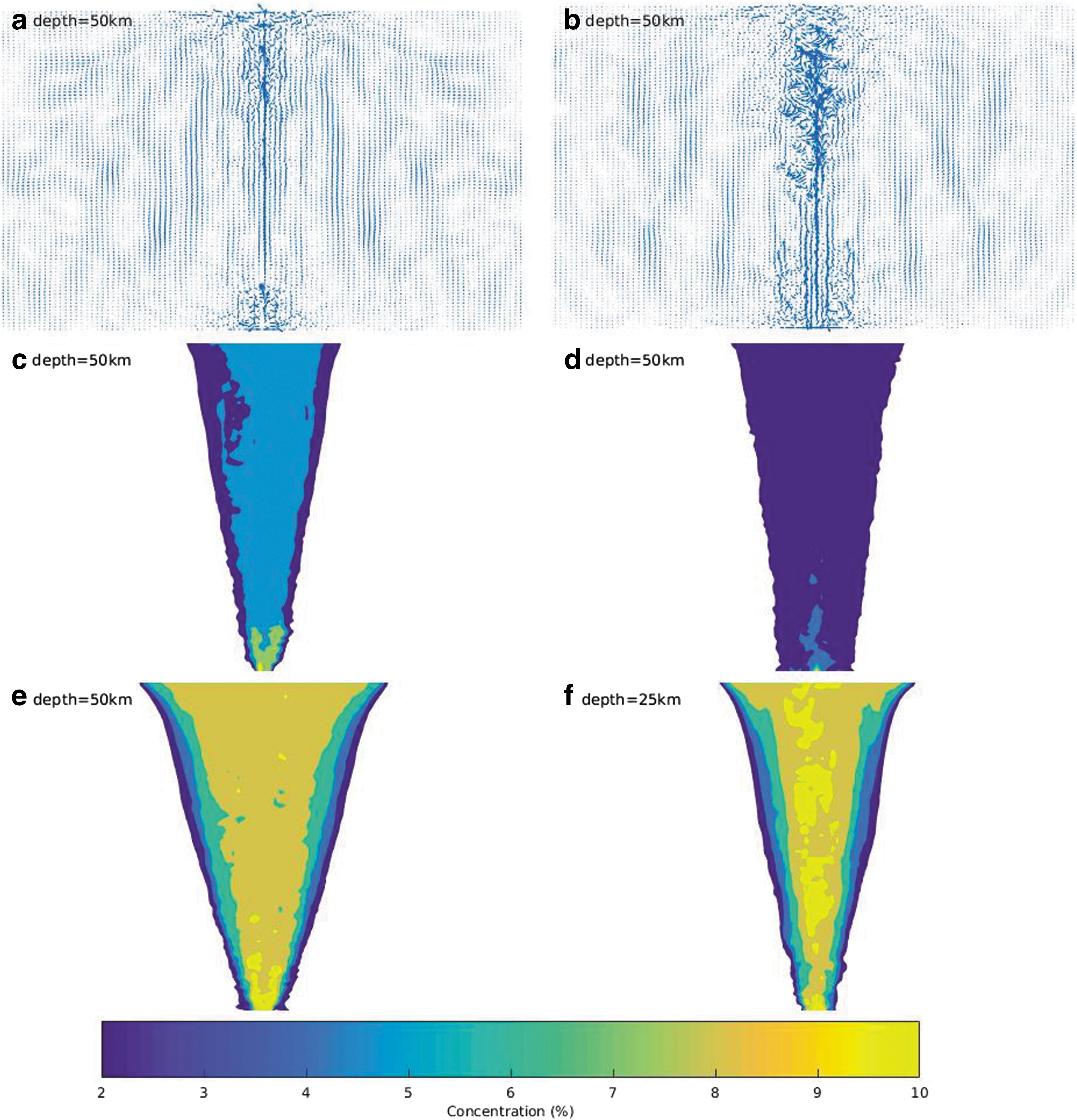
Enceladus ocean hydrothermal vent outflow model. Model domain 50 × 50 km unless specified otherwise. (a) Velocity field, H = 1.4 GW, t = 16 days; (b) Velocity field, H = 16 GW, t = 16 days; (c) Concentration, H = 1.4 GW, t = 150 days; (d) Concentration, H = 16 GW, t = 150 days; (e) Concentration, H = 1.4 GW, t = 600 days; (f) Concentration, H = 1. 4 GW, t = 150 days, Depth = 25 km.

4. Discussion

Enceladus is one of the most active bodies in the outer Solar System, with an endogenic power output close to 16 GW (Howett et al., 2011). The heat flux is primarily concentrated along the four tiger stripes and in the SPT (Spencer et al., 2006), and the power output averaged over this region is ∼400 mW/m² (Bland et al., 2012), which is almost an order of magnitude greater than the ∼50 mW/m² for the old (>50 Myr) oceanic crust on the Earth, or the 20 mW/m² calculated for the surface of Europa (Stein and Stein, 1994; Hussmann et al., 2002). Away from this region, in lower temperature areas, the endogenic heat contribution of Enceladus' surface is difficult to distinguish from passive surface heating by sunlight, and the globally averaged heat flux is estimated at 7 mW/m² (O'Neill and Nimmo, 2010; Howett et al., 2011). Cassini data suggest that the heat radiated from the SPT is drawn from the ocean below, and the release of latent heat may be the proximate energy source for the plumes (Porco et al., 2014). Temperatures measured exclude the possibility of a shallow frictional origin of this heat (Porco et al., 2014).

We assumed that the heat flux in the SPT is ultimately associated with hydrothermal activity at the ocean-core interface (Hsu et al., 2015; Sekine et al., 2015). Such hydrothermal systems are of significant astrobiological interest because they could be sites for the synthesis of organic compounds such as amino acids and nucleobases (Orgel, 2004); sugars (Ritson and Sutherland, 2012); and hydrocarbons and carboxylic acids (McCollom and Seewald, 2007), from molecules such as HCN, CH₄, and NH₃, which have been identified in plume materials (Waite et al., 2009). Alkaline hydrothermal vents have also been proposed as a possible site for the origin of life (Corliss et al., 1981; Russell et al., 1993; Martin et al., 2008). An origin of life in the Enceladus ocean may have given rise to light-independent, chemotrophic microbial communities that are associated to the vents, with methanogenic microorganisms that use CO₂ and H₂ derived from rock-water reactions (McKay et al., 2008) analogous to those that are known to thrive on the geochemical system of hydrothermal vents in the Earth's deep oceans (Stevens and McKinley, 1995; Chapelle et al., 2002). In the Earth's pre-photosynthetic biosphere, methanogen niches were most abundant where CO₂ rich ocean water flowed through serpentine (Sleep and Bird, 2007). Some of the abiotic and biotic processes that may be possible in Enceladus are summarized in Figure 3.

The availability of fresh material and its rate of alteration are essential for estimating H₂ generation in Enceladus. Our calculations indicate that serpentinization can occur globally. Malamud and Prialnik (2013) suggested that the complete differentiation of Enceladus was partially fueled by early serpentinization in the first several million years. It is recognized that the current composition of Enceladus is likely more similar to that of carbonaceous chondrites than a massive peridotitic core (Sekine et al., 2015). Unless significant heating and melting occurred during the early evolution of the satellite, these olivine rocks would not have been formed within the core. Sekine et al. (2015) experimentally demonstrated that a core similar to carbonaceous chondrites is required for the formation of nanosilica particles. The olivine-rich peridotitic composition would represent an upper limit on H₂ production.

The predicted ocean pH suggests that serpentinization might be occurring or has been occurring in the recent past (Glein et al., 2015). The presence of both H₂ and CO₂ in the plume suggests that their uptake by methanogens is not 100% efficient if biotic processes are occurring. The CO₂ suggests that the core is not well exposed to ocean circulation as (Ca,Mg)CO₃ would precipitate out.

Calculated H₂ fluxes assuredly contain a degree of uncertainty: (1) The recycling of methane could be a significant additional source of H₂ if regions of sufficient temperature exist such that it is thermodynamically favored; (2) if the extent of serpentinization is much greater than accounted for, the assumed concentration of H₂ in vent fluid would be higher; or (3) if the presence of radiolytically produced H₂ is significantly higher than in terrestrial analogues and is of significant effect on the calculated total (Lin et al., 2005, 2006). Bouquet et al. (2017) estimated radiolytic H₂ production at 0–10% of that produced by serpentinization in the current epoch.

We can compare our calculations with reported H₂/H₂O measurements in the plume of 0.4% to 1.4% (Waite et al., 2017). In our biotic model, virtually all H₂ is consumed to produce biomass, and hence, the predicted level of H₂ is at the threshold of consumption of methanogens (∼10 ppm; Kral et al., 1998). For the abiotic case, the only loss of H₂ is through the plume since, unlike organics, H₂ will not be lost due to thermal processes in the core. The measurements by Waite et al. (2017) correspond to H₂ loss rates of 1–5 × 10⁹ mol/year. Our abiotic H₂ production rates are comparable, 0.02–1 × 10⁹ mol/year from serpentinization. Thus, the measurements by Waite et al. (2017) are consistent with an abiotic ocean.

We predicted the abundance of amino acids, a proxy for the extent of organic chemical evolution in the Enceladus ocean, assuming abiotic and biotic sources. Results of the abiotic model (Fig. 5) yielded concentrations of individual amino acids up to 25 μM and total concentrations of 103.8 μM in the steady-state ocean. Abiotic processes could be further limited in their production under Enceladus' hydrothermal conditions. The study (Kebukawa et al., 2017) used to estimate production incorporated reactant concentrations that were higher than measured for Enceladus. Yanagawa and Kobayashi (1992) noted that amino acid yields would be expected to increase for reactions carried out in flow reactors where the products would be removed from the threat of thermal decomposition.

Long-term amino acid concentrations resulting from biotic sources (Fig. 5) were slightly lower than those corresponding to abiotic contributions. If biotic or abiotic sources were present, concentrations in the bulk ocean could reach a micromolar range after tens of millions of years from an initially barren ocean. Hydrolyzable amino acid concentrations of >15 and <1 μM have been reported in white smokers and the surrounding seawater, respectively, and deep ocean concentrations of ∼0.1 μM have been measured (Lee and Bada, 1977; Fuchida et al., 2014). These values are low in comparison to the estimated 90 μM steady-state concentration resulting from biotic sources in Enceladus bulk ocean water. The inferred ATP production (∼30 mg/kg) was also higher than the 5 mg/kg calculated for martian biomass production (Jakosky and Shock, 1998), and our estimates of biomass production (17 mg/kg of vent fluid) were comparable to the ∼13 mg/kg estimated for Europa (McCollom, 1999).

We also estimated an annual biomass production of 4 × 10⁴–2 × 10⁶ kg/year, and long-term average cell concentrations of 80–4250 cells/cm³, which were significantly higher than similar estimates for the Europa ocean (0.1–1 cells/cm³; Chyba and Phillips, 2001). The highly efficient biotic production assumed here (100% of the hydrothermally produced H₂), and the smaller volume of the Enceladus ocean (∼100 times less than Europa's), could account for this difference. This reasoning would also apply to the differences between amino acid, ATP, and biomass estimates for Enceladus and the values observed in terrestrial oceans. The magnitude of the biomass production that we calculated for Enceladus depends primarily on the efficiency of conversion between hydrogen and biomass. In nature, use of the hydrothermally produced hydrogen by biotic processes within the vents is unlikely to approach the 100% used here, and it may actually represent a small fraction of this total. McCollom and Shock (1997) calculated that terrestrial submarine vents provide ∼0.01 kJ/kg for methanogenesis; this is ∼5% of the 0.24 kJ/kg value that we have used.

There are at least two characteristics of amino acids that could be used to differentiate between abiotic and biotic sources: enantiomeric excess and their relative abundance with respect to glycine (Davila and McKay, 2014; Creamer et al., 2016). In the terrestrial biosphere, amino acids used in protein synthesis are l-chiral. In abiotic sources, equal production of l- and d-amino acids is expected, although enantiomeric enrichment in individual amino acids up to 15–20% has been observed in some meteorites (Cronin and Pizzarello, 1997; Pizzarello et al., 2006, 2012; Glavin et al., 2012; Pizzarello and Yarnes, 2016). The greatest enantiomeric excess measured in carbonaceous chondrites (∼20%) defines a conservative upper limit for enantiomeric excess in a pure abiotic-source scenario. Our results suggest that the initial state of the ocean will be critical in extracting a conclusive signal from enantiomeric excess.

If already populated with abiotic amino acids, then new biotic production might not bring enantiomeric excess above the abiotic baseline of ∼20%; racemization dominates new production, diluting its effect. However, racemization would be insignificant in the shortest transportation timescales from the ocean-core interface to the plume sources (Table 6). In the biotic model, unless concentrations of new vent fluid are >20% (a dilution factor <5 compared with the ∼10 calculated) in vent flow after transport to the ocean-shell interface—and preserved into the plume—the chirality of the measured solution might still lie below the abiotic threshold. For an initially amino acid-barren ocean, a chiral signature could be detected before 1–100 Myr of production, depending on the racemization rate of the specific amino acid considered.

Elevated relative concentrations of Gly are also indicative of a dominant abiotic source of amino acids, whereas over-representations of more complex amino acids such as Asp, Glu, Ser, or Val can be indicative of biotic ones (Davila and McKay, 2014; Creamer et al., 2016). Biogenic Gly production as a portion of total amino acid synthesis was ∼7%, lower than in the abiotic source (12%). Abundances relative to Gly are found from their production ratios (Table 4), with a significant difference between abiotic (0.18) and biotic (0.75) Asp relative abundances in the model. Relatively elevated concentrations of more complex amino acids (e.g., Glu, Asp) compared with Gly in plume materials could be a suitable approach to life detection.

The ocean convection model suggests that Enceladus' plume materials could be fairly representative of hydrothermal vent materials, a prediction supported by the observation that abundances of CO₂, CH_4, C₂H₂, and C₂H₄ in the plume are in excess of their aqueous solubilities (Waite et al., 2009). The ascent of the fluid column from the ocean-sediment interface may be bubble driven as well as thermally driven. The effect of this would be a shortened transport time. The estimated travel time of hydrothermal vent materials to plume sources (10–60 days) was comparable with the estimates by Hsu et al. (2015) as the maximum residence time for the nanosilica particles measured in the E-ring. The limit placed on the nanosilica mass fraction in the E-ring was ∼150–3000 ppm.

The accumulation of a dissolved silica concentration is determined experimentally and calculated theoretically by Sekine et al. (2015) under hydrothermal conditions. Under the highest pH conditions (pH >10) and temperatures of 373 K, silica concentrations of 5–10 μM (300–600 ppm) are possible. When applying the dilution factor estimated for an Enceladus ocean vent outflow, the nanosilica concentrations predicted in the plume would be 30–60 ppm. These do not overlap with, but are on the same order of, the E-ring nanosilica concentrations reported.

Due to the low circulation rates (∼10⁸ m³/year) and a relatively large ocean volume (∼10¹⁶ m³), new production is slow to be of a discernible effect on bulk ocean concentrations. The relative timescales for ocean processes are listed in Table 6. Amino acids present in the plume will be a combination of new production mixed with the background ocean; the relative concentrations of the individual species remain unchanged through mixing. The enantiomeric excess of the mixture will increase for any chiral molecules present in the new hydrothermal production. We did not take into account the effect on the concentration of bubble formation in creating the plume particles. Porco et al. (2017) have suggested that the process of bubble scrubbing could lead to significant enhancements in concentrations—by factors of 100 to 1000 s—in the plume's organic and cellular content with respect to the ocean values computed here.

5. Conclusions

We developed a model of hydrothermal production of H₂ on Enceladus and estimated the possible production of organics by both abiotic and biotic processes. We considered heat flows of 0.3 to 16 GW. The hydrological system of the ocean was represented as a vent outflow emanating from the subsurface flowing toward the SPT. This outflow was diluted by the bulk ocean. We computed the concentration of amino acids both in the bulk ocean and in the vent outflow. From these model calculations, we reached the following conclusions:

(1) Hydrothermal production of H₂ at the present time is predicted to be 0.6–34 mol/s.

(2) The concentration of amino acids in an abiotic steady-state ocean would be 104 and 90 μM in a biotic ocean scenario based on methanogens. Racemization would be complete.

(3) In the ocean hydrothermal vent outflow, only 10% of new production reaches the plume sources due to entrainment with the bulk ocean.

(4) The concentration of biotic amino acids in the plume (assuming a 10% vent contribution and a 90% bulk ocean contribution) would be 90 μM. The enantiomeric excess is <10%. Similarly, cell concentrations of ∼8.5 × 10⁷ cells/cm³ in the plume are expected.

(5) Amino acids of an exclusively abiotic origin (α-amino isobutyric acid) should reach detectable levels within the plume.

(6) For both biotic and abiotic sources, Gly is a major product. Biogenic Gly production as a portion of total amino acid synthesis was ∼7%, which was lower than from an abiotic source (12%).

The values just cited apply to the ocean. Processes that enhance the organic and cellular content in the material ascending from the ocean through the ice shell, such as bubble scrubbing, could increase the values (above) in the plume by factors of 100 to 1000 s (Porco et al., 2017). Under all models presented, total organic production was orders of magnitude lower than terrestrial production. Further experimental work to constrain the efficiency of abiotic and biogenic hydrogen conversion would be invaluable to refining the estimates used here.

Footnotes

Author Disclosure Statement

No competing financial interests exist.

Abbreviations Used

References

Adcroft

, Hill

, Campin

J.-M.

, Marshall

, and Heimbach

(2004) Overview of the formulation and numerics of the MIT GCM. In Proceedings of the ECMWF Seminar Series on Numerical Methods, Recent Developments in Numerical Methods for Atmosphere and Ocean Modelling. The European Centre for Medium-Range Weather Forecasts (ECMWF), Reading, UK; pp. 139–149.

Balme

M.R.

, Rocchi

, Jones

, Sammonds

P.R.

, Meredith

P.G.

, and Boon

(2004) Fracture toughness measurements on igneous rocks using a high-pressure, high-temperature rock fracture mechanics cell. J Volcanol Geotherm Res, 132:159–172.

Bassez

M.-P.

, Takano

, and Kobayashi

(2012) Prebiotic organic microstructures. Orig Life Evol Biosph, 42:307–316.

Bland

M.T.

, Singer

K.N.

, McKinnon

W.B.

, and Schenk

P.M.

(2012) Enceladus' extreme heat flux as revealed by its relaxed craters. Geophys Res Lett, 39:L17204; doi:10.1029/2012GL052736.

Bouhifd

M.A.

, Andrault

, Fiquet

, and Richet

(1996) Thermal expansion of forsterite up to the melting point. Geophys Res Lett, 23:1143–1146.

Bouquet

, Glein

C.R.

, Wyrick

, and Waite

J.H.

(2017) Alternative energy: production of H2 by radiolysis of water in the rocky cores of icy bodies. Astrophys J Lett. 840.

Brazelton

W.J.

, Schrenk

M.O.

, Kelley

D.S.

, and Baross

J.A.

(2006) Methane-and sulfur- metabolizing microbial communities dominate the Lost City hydrothermal field ecosystem. Appl Environ Microbiol, 72:6257–6270.

Čadek

, Tobie

, Van Hoolst

, Massé

, Choblet

, Lefèvre

, Mitri

, Baland

R.-M.

, Běhounková

, Bourgeois

, et al. (2016) Enceladus's internal ocean and ice shell constrained from Cassini gravity, shape, and libration data. Geophys Res Lett, 43:5653–5660.

Chapelle

F.H.

, O'neill

, Bradley

P.M.

, Methé

B.A.

, Ciufo

S.A.

, Knobel

L.L.

, and Lovley

D.R.

(2002) A hydrogen-based subsurface microbial community dominated by methanogens. Nature, 415:312–315.

10.

Chyba

C.F.

, and Phillips

C.B.

(2001) Possible ecosystems and the search for life on Europa. Proc Natl Acad Sci U S A, 98:801–804.

11.

Clauser

, and Huenges

(1995) Thermal conductivity of rocks and minerals. In Rock Physics & Phase Relations: A Handbook of Physical Constants, edited by Ahrens

T.J.

; American Geophysical Union, Washington, D.C., doi: 10.1029/RF003p0105; pp. 105–126.

12.

Cohen

B.A.

, and Chyba

C.F.

(2000) Racemization of meteoritic amino acids. Icarus, 145:272–281.

13.

Corliss

J.B.

, Baross

J.A.

, and Hoffman

S.E.

(1981) An hypothesis concerning the relationships between submarine hot springs and the origin of life on earth. Oceanol Acta, (special issue 6)::59–69.

14.

Creamer

J.S.

, Mora

M.F.

, and Willis

P.A.

(2016) Enhanced resolution of chiral amino acids with capillary electrophoresis for biosignature detection in extraterrestrial samples. Anal Chem, 89:1329–1337.

15.

Cronin

J.R.

, and Pizzarello

(1997) Enantiomeric excesses in meteoritic amino acids. Science, 275:951–955.

16.

Davila

A.F.

, and McKay

C.P.

(2014) Chance and necessity in biochemistry: implications for the search for extraterrestrial biomarkers in Earth-like environments. Astrobiology, 14:534–540.

17.

Decker

, Jungermann

, and Thauer

R.K.

(1970) Energy production in anaerobic organisms. Angew Chem Int Ed Engl, 9:138–158.

18.

Demartin

, Hirth

, and Evans

(2002) Experimental constraints on thermal cracking of peridotite at mid-ocean ridges. In: AGU Fall Meeting Abstracts. American Geophysical Union, Washington, D.C.

19.

Evans

A.G.

, and Clarke

D.R.

(1980) Residual stresses and microcracking induced by thermal contraction inhomogeneity. In International Conference on Thermal Stresses in Materials and Structures in Severe Thermal Environments, Blacksburg, VA, March 19–21, 1980.

20.

Field

C.B.

, Behrenfeld

M.J.

, Randerson

J.T.

, and Falkowski

(1998) Primary production of the biosphere: integrating terrestrial and oceanic components. Science, 281:237–240.

21.

Fuchida

, Mizuno

, Masuda

, Toki

, and Makita

(2014) Concentrations and distributions of amino acids in black and white smoker fluids at temperatures over 200°C. Org Geochem, 66:98–106.

22.

Glavin

D.P.

, Callahan

M.P.

, Dworkin

J.P.

, and Elsila

J.E.

(2010) The effects of parent body processes on amino acids in carbonaceous chondrites. Meteorit Planet Sci, 45:1948–1972.

23.

Glavin

D.P.

, Elsila

J.E.

, Burton

A.S.

, Callahan

M.P.

, Dworkin

J.P.

, Hilts

R.W.

, and Herd

C.D.

(2012) Unusual nonterrestrial l-proteinogenic amino acid excesses in the Tagish Lake meteorite. Meteorit Planet Sci, 47:1347–1364.

24.

Glein

C.R.

, Baross

J.A.

, and Waite

J.H.

(2015) The pH of Enceladus' ocean. Geochim Cosmochim Acta, 162:202–219.

25.

Goodman

J.C.

, and Lenferink

(2012) Numerical simulations of marine hydrothermal plumes for Europa and other icy worlds. Icarus, 221:970–983.

26.

Hansen

C.J.

, Shemansky

D.E.

, Esposito

L.W.

, Stewart

A.I.F.

, Lewis

B.R.

, Colwell

J.E.

, Hendrix

A.R.

, West

R.A.

, Waite

J.H.

Jr. , Teolis

, and Magee

B.A.

(2011) The composition and structure of the Enceladus plume. Geophys Res Lett, 38:L11202; doi:10.1029/2011GL047415.

27.

Higgs

P.G.

, and Pudritz

R.E.

(2009) A thermodynamic basis for prebiotic amino acid synthesis and the nature of the first genetic code. Astrobiology, 9:483–490.

28.

Hirose

, Kawagucci

, and Suzuki

(2011) Mechanoradical H2 generation during simulated faulting: implications for an earthquake-driven subsurface biosphere. Geophys Res Lett, 38:L17303; doi:10.1029/2011GL048850.

29.

Howett

C.J.A.

, Spencer

J.R.

, Pearl

, and Segura

(2011) High heat flow from Enceladus' south polar region measured using 10–600 cm-1 Cassini/CIRS data. J Geophys Res Planets. 116.

30.

Hsu

H.-W.

, Postberg

, Sekine

, Shibuya

, Kempf

, Horányi

, Juhász

, Altobelli

, Suzuki

, Masaki

, et al. (2015) Ongoing hydrothermal activities within Enceladus. Nature, 519:207–210.

31.

Hussmann

, Spohn

, and Wieczerkowski

(2002) Thermal equilibrium states of Europa's ice shell: implications for internal ocean thickness and surface heat flow. Icarus, 156:143–151.

32.

Iess

, Stevenson

D.J.

, Parisi

, Hemingway

, Jacobson

R.A.

, Lunine

J.I.

, Nimmo

, Armstrong

J.W.

, Asmar

S.W.

, Ducci

, and Tortora

(2014) The gravity field and interior structure of Enceladus. Science, 344,(6179)::78–80.

33.

Islam

M.N.

, Kaneko

, and Kobayashi

(2002) Determination of amino acids formed in a supercritical water flow reactor simulating submarine hydrothermal systems. Anal Sci, 17:i1631–i1634.

34.

Jakosky

B.M.

, and Shock

E.L.

(1998) The biological potential of Mars, the early Earth, and Europa. J Geophys Res Planets, 103:19359–19364.

35.

Kebukawa

, Chan

Q.H.

, Tachibana

, Kobayashi

, and Zolensky

M.E.

(2017) One-pot synthesis of amino acid precursors with insoluble organic matter in planetesimals with aqueous activity. Sci Adv, 3:p.e1602093.

36.

Khawaja

, Postberg

, Reviol

, Nölle

, Klenner

, and Srama

(2015) Identification of organics in ice grains from Enceladus. In: AGU Fall Meeting Abstracts. American Geophysical Union, Washington, D.C.

37.

Konn

, Charlou

J.-L.

, Holm

N.G.

, and Mousis

(2015) The production of methane, hydrogen, and organic compounds in ultramafic-hosted hydrothermal vents of the Mid-Atlantic ridge. Astrobiology, 15:381–399.

38.

Kral

T.A.

, Brink

K.M.

, Miller

S.L.

, and McKay

C.P.

(1998) Hydrogen consumption by methanogens on the early Earth. Orig Life Evol Biosph, 28:311–319.

39.

Lee

, and Bada

J.L.

(1977) Dissolved amino acids in the equatorial Pacific, the Sargasso Sea, and Biscayne Bay1. Limnol Oceanogr, 22:502–510.

40.

Lin

L.-H.

, Hall

, Lippmann-Pipke

, Ward

J.A.

, Sherwood Lollar

, DeFlaun

, Rothmel

, Moser

, Gihring

T.M.

, Mislowack

, and Onstott

T.C.

(2005) Radiolytic H2 in continental crust: nuclear power for deep subsurface microbial communities. Geochem Geophys Geosystems, 6:Q07003.

41.

Lin

L.-H.

, Wang

P.-L.

, Rumble

, Lippmann-Pipke

, Boice

, Pratt

L.M.

, Lollar

B.S.

, Brodie

E.L.

, Hazen

T.C.

, Andersen

G.L.

, et al. (2006) Long-term sustainability of a high-energy, low-diversity crustal biome. Science, 314:479–482.

42.

Lowell

R.P.

, and DuBose

(2005) Hydrothermal systems on Europa. Geophys Res Lett. 32.

43.

Macdonald

A.H.

, and Fyfe

W.S.

(1985) Rate of serpentinization in seafloor environments. Tectonophysics, 116:123–135.

44.

Malamud

, and Prialnik

(2013) Modeling serpentinization: applied to the early evolution of Enceladus and Mimas. Icarus, 225:763–774.

45.

Malvoisin

, Carlut

, and Brunet

(2012) Serpentinization of oceanic peridotites: 1. A high-sensitivity method to monitor magnetite production in hydrothermal experiments. J Geophys Res, 117:B01104; doi: 10.1029/2011JB008612.

46.

Martin

, Baross

, Kelley

, and Russell

M.J.

(2008) Hydrothermal vents and the origin of life. Nat Rev Microbiol, 6:805–814.

47.

McCollom

T.M.

(1999) Methanogenesis as a potential source of chemical energy for primary biomass production by autotrophic organisms in hydrothermal systems on Europa. J Geophys Res Planets, 104:30729–30742.

48.

McCollom

T.M.

(2013) The influence of minerals on decomposition of the n-alkyl-α-amino acid norvaline under hydrothermal conditions. Geochim Cosmochim Acta, 104:330–357.

49.

McCollom

T.M.

, and Amend

J.P.

(2005) A thermodynamic assessment of energy requirements for biomass synthesis by chemolithoautotrophic micro-organisms in oxic and anoxic environments. Geobiology, 3:135–144.

50.

McCollom

T.M.

, and Seewald

J.S.

(2007). Abiotic synthesis of organic compounds in deep-sea hydrothermal environments. Chem Rev, 107:382–401.

51.

McCollom

T.M.

, and Shock

E.L.

(1997) Geochemical constraints on chemolithoautotrophic metabolism by microorganisms in seafloor hydrothermal systems. Geochim Cosmochim Acta, 61:4375–4391.

52.

McKay

C.P.

, Porco

C.C.

, Altheide

, Davis

W.L.

, and Kral

T.A.

(2008) The possible origin and persistence of life on Enceladus and detection of biomarkers in the plume. Astrobiology, 8:909–919.

53.

Meyer

, and Wisdom

(2007) Tidal heating in Enceladus. Icarus, 188:535–539.

54.

Moura

, Savageau

M.A.

, and Alves

(2013) Relative amino acid composition signatures of organisms and environments. PLoS One, 8:e77319.

55.

Neveu

, Desch

S.J.

, and Castillo-Rogez

J.C.

(2015) Core cracking and hydrothermal circulation can profoundly affect Ceres' geophysical evolution. J Geophys Res Planets, 120:123–154.

56.

O'Neill

, and Nimmo

(2010) The role of episodic overturn in generating the surface geology and heat flow on Enceladus. Nat Geosci, 3:88–91.

57.

Orgel

L.E.

(2004) Prebiotic chemistry and the origin of the RNA world. Crit Rev Biochem Mol Biol, 39:99–123.

58.

Pizzarello

, and Yarnes

C.T.

(2016) Enantiomeric excesses of chiral amines in ammonia-rich carbonaceous meteorites. Earth Planet Sci Lett, 443:176–184.

59.

Pizzarello

, Cooper

G.W.

, and Flynn

G.J.

(2006) The nature and distribution of the organic material in carbonaceous chondrites and interplanetary dust particles. In Meteorites and the Early Solar System II, 1, edited by Lauretta

D.S.

and McSween

H.Y.

, University of Arizona Press, Tucson; pp. 625–651.

60.

Pizzarello

, Schrader

D.L.

, Monroe

A.A.

, and Lauretta

D.S.

(2012) Large enantiomeric excesses in primitive meteorites and the diverse effects of water in cosmochemical evolution. Proc Natl Acad Sci U S A, 109:11949–11954.

61.

Porco

, DiNino

, and Nimmo

(2014) How the geysers, tidal stresses, and thermal emission across the south polar terrain of Enceladus are related. Astron J, 148:45.

62.

Porco

, Dones

, and Mitchell

(2017) Could it be snowing microbes on Enceladus? Assessing conditions in its plume and implications for future missions. Astrobiology, 17:876–901.

63.

Porco

C.C.

, Helfenstein

, Thomas

P.C.

, Ingersoll

A.P.

, Wisdom

, West

, Neukum

, Denk

, Wagner

, Roatsch

, et al. (2006) Cassini observes the active south pole of Enceladus. Science, 311:1393–1401.

64.

Postberg

, Khawaja

, Hsu

H.W.

, Sekine

, and Shibuya

(2015) Refractory organic compounds in Enceladus' ice grains and hydrothermal activity. In AGU Fall Meeting Abstracts. American Geophysical Union, Washington, D.C.

65.

Postberg

, Schmidt

, Hillier

, Kempf

, and Srama

(2011) A salt-water reservoir as the source of a compositionally stratified plume on Enceladus. Nature, 474:620–622.

66.

Ritson

, Sutherland

J.D.

, 2012. Prebiotic synthesis of simple sugars by photoredox systems chemistry. Nat Chem, 4, 895–899.

67.

Russell

M.J.

, Daniel

R.M.

, and Hall

A.J.

(1993) On the emergence of life via catalytic iron-sulphide membranes. Terra Nova, 5:343–347.

68.

Sekine

, Shibuya

, Postberg

, Hsu

H.-W.

, Suzuki

, Masaki

, Kuwatani

, Mori

, Hong

P.K.

, Yoshizaki

, Tachibana

, and Sirono

(2015) High-temperature water–rock interactions and hydrothermal environments in the chondrite-like core of Enceladus. Nat Commun, 6:8604; doi:10.1038/ncomms9604.

69.

Sherwood Lollar

, Voglesonger

, Lin

L.-H.

, Lacrampe-Couloume

, Telling

, Abrajano

T.A.

, Onstott

T.C.

, and Pratt

L.M.

(2007). Hydrogeologic controls on episodic H2 release from Precambrian fractured rocks—energy for deep subsurface life on Earth and Mars. Astrobiology, 7:971–986.

70.

Sleep

N.H.

, and Bird

D.K.

(2007) Niches of the pre-photosynthetic biosphere and geologic preservation of Earth's earliest ecology. Geobiology, 5:101–117.

71.

Sleep

N.H.

, Bird

D.K.

, and Pope

E.C.

(2011) Serpentinite and the dawn of life. Philos Trans R Soc Lond B Biol Sci, 366:2857–2869.

72.

Sleep

N.H.

, Meibom

, Fridriksson

, Coleman

R.G.

, and Bird

D.K.

(2004) H2-rich fluids from serpentinization: geochemical and biotic implications. Proc Natl Acad Sci U S A, 101:12818–12823.

73.

Spencer

J.R.

, Pearl

J.C.

, Segura

, Flasar

F.M.

, Mamoutkine

, Romani

, Buratti

B.J.

, Hendrix

A.R.

, Spilker

L.J.

, and Lopes

R.M.C.

(2006). Cassini encounters Enceladus: background and the discovery of a south polar hot spot. Science, 311:1401–1405.

74.

Stein

C.A.

and Stein

(1994) Constraints on hydrothermal heat flux through the oceanic lithosphere from global heat flow. J Geophys Res, 99:3081–3095.

75.

Stevens

T.O.

, and McKinley

J.P.

(1995) Lithoautotrophic microbial ecosystems in deep basalt aquifers. Science, 270:450.

76.

Thauer

R.K.

, Jungermann

, and Decker

(1977) Energy conservation in chemotrophic anaerobic bacteria. Bacteriol Rev, 41:100.

77.

Toggweiler

J.R.

, and Robert

M.K.

(2001) Ocean circulation/thermohaline circulation. In Encyclopedia of Atmospheric Sciences, Vol. 4. Academic Press, San Diego, pp.1549–1555.

78.

Vance

, Harnmeijer

, Kimura

, Hussmann

, DeMartin

, and Brown

J.M.

(2007) Hydrothermal systems in small ocean planets. Astrobiology, 7:987–1005.

79.

Vance

S.D.

, Hand

K.P.

, and Pappalardo

R.T.

(2016) Geophysical controls of chemical disequilibria in Europa. Geophys Res Lett, 43:4871–4879.

80.

Waite

J.H.

, Glein

C.R.

, Perryman

R.S.

, Teolis

B.D.

, Magee

B.A.

, Miller

, Grimes

, Perry

M.E.

, Miller

K.E.

, Bouquet

, and Lunine

J.I.

(2017) Cassini finds molecular hydrogen in the Enceladus plume: evidence for hydrothermal processes. Science, 356:155–159.

81.

Waite

J.H.

Jr , Lewis

W.S.

, Magee

B.A.

, Lunine

J.I.

, McKinnon

W.B.

, Glein

C.R.

, Mousis

, Young

D.T.

, Brockwell

, Westlake

, et al. (2009) Liquid water on Enceladus from observations of ammonia and 40Ar in the plume. Nature, 460:487–490.

82.

Whitman

W.B.

, Coleman

D.C.

, and Wiebe

W.J.

(1998) Prokaryotes: the unseen majority. Proc Natl Acad Sci U S A, 95:6578–6583.

83.

Yablokov

V.A.

, Smel'tsova

I.L.

, and Faerman

V.I.

(2013) Thermal stability of amino acids. Russ J Gen Chem, 83:476–480.

84.

Yanagawa

, and Kobayashi

(1992) Chapter 8 an experimental approach to chemical evolution in submarine hydrothermal systems. Orig Life Evol Biosph, 22:147–159.