The ability to support a replicator population in an extremely hostile environment is considered in a simple model of a prebiotic cell. We explore from a classical approach how the replicator viability changes as a function of the cell radius. The model includes the interaction between two different species: a substrate that flows from the exterior and a replicator that feeds on the substrate and is readily destroyed in the environment outside the cell. According to our results, replicators in the cell only exist when the radius exceeds some critical value \documentclass{aastex}\usepackage{amsbsy}\usepackage{amsfonts}\usepackage{amssymb}\usepackage{bm}\usepackage{mathrsfs}\usepackage{pifont}\usepackage{stmaryrd}\usepackage{textcomp}\usepackage{portland, xspace}\usepackage{amsmath, amsxtra}\usepackage{upgreek}\pagestyle{empty}\DeclareMathSizes{10}{9}{7}{6}\begin{document}$$\left( {{R_{ \rm{C}}} \le R} \right)$$ \end{document} being, in general, a function of the substrate concentration, the diffusion constant of the replicator species, and the reproduction rate coefficient. Additionally, the influence of other parameters on the replicator population is also considered. The viability of chemical replicators under such drastic conditions could be crucial in understanding the origin of the first primitive cells and the ulterior development of life on our planet. Key Words: Prebiotic cell—Chemical replicator—Environment—Reproduction rate. Astrobiology 18, 403–411.
1. Introduction
Contemporary forms of life are an outcome of a very long process of evolution that began relatively early on ancient Earth. Among natural phenomena, contemporary life differs noticeably from other nonliving processes that have taken place on Earth and has shown fascinating diversity and a noticeable degree of complexity (Schrödinger, 1967; Lazcano, 2008). Intrinsic features such as the ability to self-replicate, to be self-sustained, and to experience Darwinian evolution locate it in a special place in the universe of all known physicochemical processes.
However, despite the inner complexity displayed by contemporary cells, it is presumable that the first rudimentary forms of life were extremely simple compared to extant life-forms at present. This idea opens the possibility of exploring some nonliving systems of minimal complexity, namely, “infrabiological systems,” which could be key to understanding genesis on Earth and the ulterior development of life. Regrettably, even though many different hypotheses and theories have been proposed (King, 1982; Maynard-Smith, 1979; Wächtershäuser, 2007; Schrum et al.,2010; Robertson and Joyce, 2012), there is no consensus in the scientific community as to how this process of abiogenesis took place.
As a rule, most of the theories about the origin of life emphasize one or another element of the life phenomenon relegating the relevance of the others. This is the case for well-known theories such as those that have to do with the RNA world and “metabolism first” (Gilbert, 1986; Bartel and Unrau, 1999; Anet, 2004; Robertson and Joyce, 2012). Issues such as the abiotic synthesis of organic compounds (Ferris, 2005; Brack, 2007; Ehrenfreund et al.,2011), the origin of the first replicator systems (Szathmáry and Demeter, 1987; Czárán and Szathmáry, 2000; Szathmáry, 2006; Hernandez and Grover, 2013), and associated thermodynamic requirements (Kleidon, 2010; Boiteau and Pascal, 2011; Dobovišek et al.,2011; England, 2013) have become recurrent topics in these studies. In the same way, a considerable number of works have focused on the specific role played by primitive membranes and the processes of vesicle formation in the structures that preceded the emergence of the first forms of life (Morowitz et al.,1988; Martín et al.,2009; Schrum et al.,2010; Könnyű and Czárán, 2013; Walde et al.,2014; Sakuma and Imai, 2015). Beyond differences among respective approaches, they all represent a notable effort in the search for what we could call the essence of the life phenomenon (Benner, 2010; Chodasewicz, 2014; Ma, 2016).
In our case, we are interested in the potential of organic vesicles to harbor a population of an elemental chemical replicator, a process that could be considered as a very early step in the process of abiogenesis (Ma and Feng, 2015). In some way, this scenario combines two distinctive elements of contemporary life: on one hand, the existence of a membranous cell boundary delimiting the cell shape and controlling the exchange of metabolites and energy between the cell and the environment; on the other hand, the necessity of continued replication as the way to preserve the cell in a dynamics steady state (Pross, 2005b). This last feature is essential for preserving the functioning of cellular structures against the impact of many different processes like the consumption associated with metabolism or, simply, molecular degradation.
In general, the idea to confine the process of chemical replication to the interior of a vesicle raises many different questions. Is a replicator population inside a vesicle always viable? Which are the key factors that control this process? How may the availability of nutrients affect the overall process? These are some of the basic questions that have driven the development of this work.
2. The Model
As a model of the prebiotic cell, we considered a spherical vesicle delimited by a selective membrane. The vesicle is immersed in a medium where the content of nutrients remains constant. Two different chemical species are considered in our analysis. On one hand, a substrate \documentclass{aastex}\usepackage{amsbsy}\usepackage{amsfonts}\usepackage{amssymb}\usepackage{bm}\usepackage{mathrsfs}\usepackage{pifont}\usepackage{stmaryrd}\usepackage{textcomp}\usepackage{portland, xspace}\usepackage{amsmath, amsxtra}\usepackage{upgreek}\pagestyle{empty}\DeclareMathSizes{10}{9}{7}{6}\begin{document}$$\left( u \right)$$ \end{document} that flows by diffusion into the cell from the exterior; on the other hand, a replicator \documentclass{aastex}\usepackage{amsbsy}\usepackage{amsfonts}\usepackage{amssymb}\usepackage{bm}\usepackage{mathrsfs}\usepackage{pifont}\usepackage{stmaryrd}\usepackage{textcomp}\usepackage{portland, xspace}\usepackage{amsmath, amsxtra}\usepackage{upgreek}\pagestyle{empty}\DeclareMathSizes{10}{9}{7}{6}\begin{document}$$\left( v \right)$$ \end{document} that feeds on the substrate and is readily destroyed in the external medium surrounding the vesicle. The model does not include an explicit coupling between the vesicle and the replication process that occurs in the cell interior. In this sense, the vesicle environment acts as a small reactor limiting the replication process to the inner volume (Ma and Feng, 2015). The equations governing the dynamics of the system are the following:\documentclass{aastex}\usepackage{amsbsy}\usepackage{amsfonts}\usepackage{amssymb}\usepackage{bm}\usepackage{mathrsfs}\usepackage{pifont}\usepackage{stmaryrd}\usepackage{textcomp}\usepackage{portland, xspace}\usepackage{amsmath, amsxtra}\usepackage{upgreek}\pagestyle{empty}\DeclareMathSizes{10}{9}{7}{6}\begin{document} \begin{align*}{ \frac { \partial u } { \partial t } } = { D_1 } \left( { { \frac { { \partial ^2 } u } { \partial { r^2 } } } + \frac { 2 } { r } { \frac { \partial u } { \partial r } } } \right) - a \;uv = 0 \tag { 1 } \end{align*} \end{document}\documentclass{aastex}\usepackage{amsbsy}\usepackage{amsfonts}\usepackage{amssymb}\usepackage{bm}\usepackage{mathrsfs}\usepackage{pifont}\usepackage{stmaryrd}\usepackage{textcomp}\usepackage{portland, xspace}\usepackage{amsmath, amsxtra}\usepackage{upgreek}\pagestyle{empty}\DeclareMathSizes{10}{9}{7}{6}\begin{document} \begin{align*}{ \frac { \partial v } { \partial t } } = { D_2 } \left( { { \frac { { \partial ^2 } v } { \partial { r^2 } } } + \frac { 2 } { r } { \frac { \partial v } { \partial r } } } \right) + a \;uv - { d_n } \; { v^n } = 0 \quad \quad n = 1 , \;2 \tag { 2 } \end{align*} \end{document}
where D1 and D2 are the diffusion constants for each species and the parameters a and \documentclass{aastex}\usepackage{amsbsy}\usepackage{amsfonts}\usepackage{amssymb}\usepackage{bm}\usepackage{mathrsfs}\usepackage{pifont}\usepackage{stmaryrd}\usepackage{textcomp}\usepackage{portland, xspace}\usepackage{amsmath, amsxtra}\usepackage{upgreek}\pagestyle{empty}\DeclareMathSizes{10}{9}{7}{6}\begin{document}$${d_n} = \left\{ {{d_1} , {d_2}} \right\} $$ \end{document} are the reproduction and mortality (first and second order) rate constants, respectively. Two different alternatives were considered in modeling the decay of the replicator population according to the value of n used in Eq. 2. When \documentclass{aastex}\usepackage{amsbsy}\usepackage{amsfonts}\usepackage{amssymb}\usepackage{bm}\usepackage{mathrsfs}\usepackage{pifont}\usepackage{stmaryrd}\usepackage{textcomp}\usepackage{portland, xspace}\usepackage{amsmath, amsxtra}\usepackage{upgreek}\pagestyle{empty}\DeclareMathSizes{10}{9}{7}{6}\begin{document}$$n = 1$$ \end{document}, a linear decay of the form \documentclass{aastex}\usepackage{amsbsy}\usepackage{amsfonts}\usepackage{amssymb}\usepackage{bm}\usepackage{mathrsfs}\usepackage{pifont}\usepackage{stmaryrd}\usepackage{textcomp}\usepackage{portland, xspace}\usepackage{amsmath, amsxtra}\usepackage{upgreek}\pagestyle{empty}\DeclareMathSizes{10}{9}{7}{6}\begin{document}$$( - {d_1}v )$$ \end{document} is assumed, representing the intrinsic degradation rate of the replicator. A linear decay is presumably the right choice for such replicator systems where the spontaneous, thermal, or photolytic decomposition plays a major role. On the other hand, a nonlinear decay of the form \documentclass{aastex}\usepackage{amsbsy}\usepackage{amsfonts}\usepackage{amssymb}\usepackage{bm}\usepackage{mathrsfs}\usepackage{pifont}\usepackage{stmaryrd}\usepackage{textcomp}\usepackage{portland, xspace}\usepackage{amsmath, amsxtra}\usepackage{upgreek}\pagestyle{empty}\DeclareMathSizes{10}{9}{7}{6}\begin{document}$$( - {d_2} \;{v^2} )$$ \end{document} when \documentclass{aastex}\usepackage{amsbsy}\usepackage{amsfonts}\usepackage{amssymb}\usepackage{bm}\usepackage{mathrsfs}\usepackage{pifont}\usepackage{stmaryrd}\usepackage{textcomp}\usepackage{portland, xspace}\usepackage{amsmath, amsxtra}\usepackage{upgreek}\pagestyle{empty}\DeclareMathSizes{10}{9}{7}{6}\begin{document}$$n = 2$$ \end{document} is associated with the underlying chemistry of the system. In this particular case, we presume the formation of a new inactive chemical species in the reaction of two replicator molecules. Nowadays, the processes that lead to new polymeric species (dimers, trimers, and so on) are considered relevant in the process of augmenting the complexity that preceded the emergence of the first forms of life (Sandars, 2003; Walker et al.,2012). However, only a reduced number of polymers that likely formed at very early stages represent an evolutionary advantage, with most of them being nonfunctional species. Hereinafter, we denominate as the M1 model when the decay law in Eq. 2 is linear \documentclass{aastex}\usepackage{amsbsy}\usepackage{amsfonts}\usepackage{amssymb}\usepackage{bm}\usepackage{mathrsfs}\usepackage{pifont}\usepackage{stmaryrd}\usepackage{textcomp}\usepackage{portland, xspace}\usepackage{amsmath, amsxtra}\usepackage{upgreek}\pagestyle{empty}\DeclareMathSizes{10}{9}{7}{6}\begin{document}$$\left( {n = 1} \right)$$ \end{document} and the M2 model when the considered decay is nonlinear \documentclass{aastex}\usepackage{amsbsy}\usepackage{amsfonts}\usepackage{amssymb}\usepackage{bm}\usepackage{mathrsfs}\usepackage{pifont}\usepackage{stmaryrd}\usepackage{textcomp}\usepackage{portland, xspace}\usepackage{amsmath, amsxtra}\usepackage{upgreek}\pagestyle{empty}\DeclareMathSizes{10}{9}{7}{6}\begin{document}$$\left( {n = 2} \right).$$ \end{document}
The boundary conditions assume that the substrate concentration remains constant at the cell radius \documentclass{aastex}\usepackage{amsbsy}\usepackage{amsfonts}\usepackage{amssymb}\usepackage{bm}\usepackage{mathrsfs}\usepackage{pifont}\usepackage{stmaryrd}\usepackage{textcomp}\usepackage{portland, xspace}\usepackage{amsmath, amsxtra}\usepackage{upgreek}\pagestyle{empty}\DeclareMathSizes{10}{9}{7}{6}\begin{document}$$\left( {u \left( R \right) = {u_0}} \right)$$ \end{document}, whereas the replicator concentration is null \documentclass{aastex}\usepackage{amsbsy}\usepackage{amsfonts}\usepackage{amssymb}\usepackage{bm}\usepackage{mathrsfs}\usepackage{pifont}\usepackage{stmaryrd}\usepackage{textcomp}\usepackage{portland, xspace}\usepackage{amsmath, amsxtra}\usepackage{upgreek}\pagestyle{empty}\DeclareMathSizes{10}{9}{7}{6}\begin{document}$$\left( {v \left( R \right) = 0} \right)$$ \end{document} as a consequence of the hostile environment outside the cell membrane. Also, it is assumed that both species remain finite at the vesicle center \documentclass{aastex}\usepackage{amsbsy}\usepackage{amsfonts}\usepackage{amssymb}\usepackage{bm}\usepackage{mathrsfs}\usepackage{pifont}\usepackage{stmaryrd}\usepackage{textcomp}\usepackage{portland, xspace}\usepackage{amsmath, amsxtra}\usepackage{upgreek}\pagestyle{empty}\DeclareMathSizes{10}{9}{7}{6}\begin{document}$$\left( \frac{\partial u} {\partial r } {\vert _ { r= 0 } } = { \frac {\partial v } { \partial r } {{ \vert _ { r = 0} } = 0 }} \right).$$ \end{document} In fact, the second assumption \documentclass{aastex}\usepackage{amsbsy}\usepackage{amsfonts}\usepackage{amssymb}\usepackage{bm}\usepackage{mathrsfs}\usepackage{pifont}\usepackage{stmaryrd}\usepackage{textcomp}\usepackage{portland, xspace}\usepackage{amsmath, amsxtra}\usepackage{upgreek}\pagestyle{empty}\DeclareMathSizes{10}{9}{7}{6}\begin{document}$$\left( {v \left( R \right) = 0} \right)$$ \end{document} determines an extreme limit where the molecules of replicators are quickly degraded or inhibited due to a variety of physical and chemical agents present in the external medium. In this sense, the vesicle plays a major role in stabilizing physical conditions (for instance, reducing the UV levels) and impeding the input of strange compounds that are able to interrupt the replication mechanism inside the cell (Del Bianco and Mansy, 2012). This last feature could be crucial in preserving the integrity of the replication mechanism inside the cell, taking into account the large number of different chemicals that can be produced (King, 1982; Patel et al.,2015) as a consequence of the complexity of the chemical network and the continuous stochastic fluctuations of the environmental conditions. For milder scenarios, the replicator concentrations may fall exponentially beyond the vesicle radius, increasing the possibility of disseminating in the medium.
Basically, we are interested in the possibilities of the former system (with the M1 or M2 model) of having additional steady states where \documentclass{aastex}\usepackage{amsbsy}\usepackage{amsfonts}\usepackage{amssymb}\usepackage{bm}\usepackage{mathrsfs}\usepackage{pifont}\usepackage{stmaryrd}\usepackage{textcomp}\usepackage{portland, xspace}\usepackage{amsmath, amsxtra}\usepackage{upgreek}\pagestyle{empty}\DeclareMathSizes{10}{9}{7}{6}\begin{document}$$\left\{ {v \left( r \right) > 0} \right\} $$ \end{document} as an alternative to the null solution. For the sake of simplicity, we nondimensionalize the former system, introducing the following transformations:\documentclass{aastex}\usepackage{amsbsy}\usepackage{amsfonts}\usepackage{amssymb}\usepackage{bm}\usepackage{mathrsfs}\usepackage{pifont}\usepackage{stmaryrd}\usepackage{textcomp}\usepackage{portland, xspace}\usepackage{amsmath, amsxtra}\usepackage{upgreek}\pagestyle{empty}\DeclareMathSizes{10}{9}{7}{6}\begin{document} \begin{align*} u = { C_0 } { \frac { { { \widetilde u } _r } } { \widetilde r } } ; \;v = { C_0 } ^ { 3 - n } \frac { a } { { { d_n } } } { \frac { { { \widetilde v } _r } } { \; \widetilde r { \rm { \; } } } } ; \;r\, = { \left( { { \frac { { D_2 } } { a \; { C_0 } \; } } } \right) ^ { \frac { 1 } { 2 } } } \; \widetilde r \tag { 3 } \end{align*} \end{document}
Where \documentclass{aastex}\usepackage{amsbsy}\usepackage{amsfonts}\usepackage{amssymb}\usepackage{bm}\usepackage{mathrsfs}\usepackage{pifont}\usepackage{stmaryrd}\usepackage{textcomp}\usepackage{portland, xspace}\usepackage{amsmath, amsxtra}\usepackage{upgreek}\pagestyle{empty}\DeclareMathSizes{10}{9}{7}{6}\begin{document}$${ \widetilde u_r} , \,\;\;{ \widetilde v_r}$$ \end{document} are auxiliary variables, the ratios \documentclass{aastex}\usepackage{amsbsy}\usepackage{amsfonts}\usepackage{amssymb}\usepackage{bm}\usepackage{mathrsfs}\usepackage{pifont}\usepackage{stmaryrd}\usepackage{textcomp}\usepackage{portland, xspace}\usepackage{amsmath, amsxtra}\usepackage{upgreek}\pagestyle{empty}\DeclareMathSizes{10}{9}{7}{6}\begin{document}$$\widetilde u = { \frac { \textstyle { { \widetilde u } _r } } { \textstyle\widetilde r } } $$ \end{document} and \documentclass{aastex}\usepackage{amsbsy}\usepackage{amsfonts}\usepackage{amssymb}\usepackage{bm}\usepackage{mathrsfs}\usepackage{pifont}\usepackage{stmaryrd}\usepackage{textcomp}\usepackage{portland, xspace}\usepackage{amsmath, amsxtra}\usepackage{upgreek}\pagestyle{empty}\DeclareMathSizes{10}{9}{7}{6}\begin{document}$$\widetilde v = { \textstyle \frac { { { \widetilde v } _r } } { \textstyle \widetilde r } } $$ \end{document} are the corresponding nondimensional concentrations, whereas the new term C0 codifies the unit of concentration used in the analysis. Thus, the system of Eqs. 1 and 2 can be written as\documentclass{aastex}\usepackage{amsbsy}\usepackage{amsfonts}\usepackage{amssymb}\usepackage{bm}\usepackage{mathrsfs}\usepackage{pifont}\usepackage{stmaryrd}\usepackage{textcomp}\usepackage{portland, xspace}\usepackage{amsmath, amsxtra}\usepackage{upgreek}\pagestyle{empty}\DeclareMathSizes{10}{9}{7}{6}\begin{document} \begin{align*} \left( { { \frac { { D_1 } } { { D_2 } } } } \right) \left( { { \frac { { d_n } } { a \; { C_0 } ^ { 2 - n } } } } \right) \; { \frac { { \partial ^2 } { { \widetilde u } _r } } { \partial { { \widetilde r } ^2 } } } - \; { \frac { { { \widetilde u } _r } { { \widetilde v } _r } } { \widetilde r } } = 0 \tag { 4 } \end{align*} \end{document}\documentclass{aastex}\usepackage{amsbsy}\usepackage{amsfonts}\usepackage{amssymb}\usepackage{bm}\usepackage{mathrsfs}\usepackage{pifont}\usepackage{stmaryrd}\usepackage{textcomp}\usepackage{portland, xspace}\usepackage{amsmath, amsxtra}\usepackage{upgreek}\pagestyle{empty}\DeclareMathSizes{10}{9}{7}{6}\begin{document} \begin{align*}{ \frac { { \partial ^2 } \widetilde v } { \partial { { \widetilde r } ^2 } } } + \; { \frac { { { \widetilde u } _r } { { \widetilde v } _r } } { \widetilde r } } - { \left( { { \frac { { d_n } } { a \; { C_0 } } } } \right) ^ { 2 - n } } { \widetilde v_r } ^n = 0 \quad \quad { \rm with } \ n = 1 , \; 2 \tag { 5 } \end{align*} \end{document}
The boundary conditions consistent with the new parameterization are the following:\documentclass{aastex}\usepackage{amsbsy}\usepackage{amsfonts}\usepackage{amssymb}\usepackage{bm}\usepackage{mathrsfs}\usepackage{pifont}\usepackage{stmaryrd}\usepackage{textcomp}\usepackage{portland, xspace}\usepackage{amsmath, amsxtra}\usepackage{upgreek}\pagestyle{empty}\DeclareMathSizes{10}{9}{7}{6}\begin{document} \begin{align*}{ \widetilde u_r} \left( { \widetilde R} \right) = { \widetilde u_0}; \;{ \widetilde v_r} \left( { \widetilde R} \right) = 0 \tag{6} \end{align*} \end{document}\documentclass{aastex}\usepackage{amsbsy}\usepackage{amsfonts}\usepackage{amssymb}\usepackage{bm}\usepackage{mathrsfs}\usepackage{pifont}\usepackage{stmaryrd}\usepackage{textcomp}\usepackage{portland, xspace}\usepackage{amsmath, amsxtra}\usepackage{upgreek}\pagestyle{empty}\DeclareMathSizes{10}{9}{7}{6}\begin{document} \begin{align*}{ \widetilde u_r} \left( 0 \right) = 0; \;{ \widetilde v_r} \left( 0 \right) = 0 \tag{7} \end{align*} \end{document}
Additionally, for completeness, we also consider a limiting case in the context of the M2 model, when the diffusion rate of the substrate is considered infinity. In this specific case, the system (Eqs. 4 and 5 for \documentclass{aastex}\usepackage{amsbsy}\usepackage{amsfonts}\usepackage{amssymb}\usepackage{bm}\usepackage{mathrsfs}\usepackage{pifont}\usepackage{stmaryrd}\usepackage{textcomp}\usepackage{portland, xspace}\usepackage{amsmath, amsxtra}\usepackage{upgreek}\pagestyle{empty}\DeclareMathSizes{10}{9}{7}{6}\begin{document}$$n = 2$$ \end{document}) is reduced formally to the Fisher-Kolmogorov equation (Fisher, 1930) (hereinafter the F-K equation), which determines the dynamics of the replicator species (Eq. 8)\documentclass{aastex}\usepackage{amsbsy}\usepackage{amsfonts}\usepackage{amssymb}\usepackage{bm}\usepackage{mathrsfs}\usepackage{pifont}\usepackage{stmaryrd}\usepackage{textcomp}\usepackage{portland, xspace}\usepackage{amsmath, amsxtra}\usepackage{upgreek}\pagestyle{empty}\DeclareMathSizes{10}{9}{7}{6}\begin{document} \begin{align*}{ \frac { { \partial ^2 } { { \widetilde v } _r } } { \partial { { \widetilde r } ^2 } } } + { \widetilde u_0 } \; { \widetilde v_r } - { \frac { { { \widetilde v } _r } ^2 } { \widetilde r } } = 0 \tag { 8 } \end{align*} \end{document}
where the concentration of substrate in the medium \documentclass{aastex}\usepackage{amsbsy}\usepackage{amsfonts}\usepackage{amssymb}\usepackage{bm}\usepackage{mathrsfs}\usepackage{pifont}\usepackage{stmaryrd}\usepackage{textcomp}\usepackage{portland, xspace}\usepackage{amsmath, amsxtra}\usepackage{upgreek}\pagestyle{empty}\DeclareMathSizes{10}{9}{7}{6}\begin{document}$${ \widetilde u_0}$$ \end{document} behaves as an effective reproduction rate constant. The boundary conditions in this new situation remain unchanged (equations in 7). The F-K equation has been broadly applied to the modeling in very different contexts, including genetics (Fisher, 1930; Pigolotti et al.,2012), ecology (Artiles et al.,2008; Giometto et al.,2014), and chemistry (Schwartz and Solomon, 2008).
Our basic program includes two main steps. Firstly, we explore the existence of a critical radius \documentclass{aastex}\usepackage{amsbsy}\usepackage{amsfonts}\usepackage{amssymb}\usepackage{bm}\usepackage{mathrsfs}\usepackage{pifont}\usepackage{stmaryrd}\usepackage{textcomp}\usepackage{portland, xspace}\usepackage{amsmath, amsxtra}\usepackage{upgreek}\pagestyle{empty}\DeclareMathSizes{10}{9}{7}{6}\begin{document}$${ \widetilde R_{ \rm{C}}}$$ \end{document} for both models (M1 and M2) under which the population of replicators is no longer viable inside the vesicle. Secondly, we examine how an already established population of replicators could be affected by plausible changes in the values of the parameters. Basically, we are going to consider the impact of possible differences in the diffusion rate constants between both species \documentclass{aastex}\usepackage{amsbsy}\usepackage{amsfonts}\usepackage{amssymb}\usepackage{bm}\usepackage{mathrsfs}\usepackage{pifont}\usepackage{stmaryrd}\usepackage{textcomp}\usepackage{portland, xspace}\usepackage{amsmath, amsxtra}\usepackage{upgreek}\pagestyle{empty}\DeclareMathSizes{10}{9}{7}{6}\begin{document}$$\big ( { { \frac { { D_1 } } { { D_2 } } } } \big )$$ \end{document}, changes in the balance between death and birth processes \documentclass{aastex}\usepackage{amsbsy}\usepackage{amsfonts}\usepackage{amssymb}\usepackage{bm}\usepackage{mathrsfs}\usepackage{pifont}\usepackage{stmaryrd}\usepackage{textcomp}\usepackage{portland, xspace}\usepackage{amsmath, amsxtra}\usepackage{upgreek}\pagestyle{empty}\DeclareMathSizes{10}{9}{7}{6}\begin{document}$$ \left( \displaystyle { { \frac { { d_n } } { a \; { C_0 } ^ { 2 - n } } } } \right)$$ \end{document}, the availability of the substrate at the cell boundary \documentclass{aastex}\usepackage{amsbsy}\usepackage{amsfonts}\usepackage{amssymb}\usepackage{bm}\usepackage{mathrsfs}\usepackage{pifont}\usepackage{stmaryrd}\usepackage{textcomp}\usepackage{portland, xspace}\usepackage{amsmath, amsxtra}\usepackage{upgreek}\pagestyle{empty}\DeclareMathSizes{10}{9}{7}{6}\begin{document}$$( { \widetilde u_0} )$$ \end{document}, and the size of the cell \documentclass{aastex}\usepackage{amsbsy}\usepackage{amsfonts}\usepackage{amssymb}\usepackage{bm}\usepackage{mathrsfs}\usepackage{pifont}\usepackage{stmaryrd}\usepackage{textcomp}\usepackage{portland, xspace}\usepackage{amsmath, amsxtra}\usepackage{upgreek}\pagestyle{empty}\DeclareMathSizes{10}{9}{7}{6}\begin{document}$$\left( { \widetilde R} \right)$$ \end{document}. The main similarities and differences between the results obtained from the application of the M1 or M2 model are discussed in all studied cases.
3. Results and Analysis
3.1. Factors conditioning the existence of a critical radius \documentclass{aastex}\usepackage{amsbsy}\usepackage{amsfonts}\usepackage{amssymb}\usepackage{bm}\usepackage{mathrsfs}\usepackage{pifont}\usepackage{stmaryrd}\usepackage{textcomp}\usepackage{portland, xspace}\usepackage{amsmath, amsxtra}\usepackage{upgreek}\pagestyle{empty}\DeclareMathSizes{10}{9}{7}{6}\begin{document}$${{{\widetilde R}}_{C}}$$ \end{document}
Firstly, we examine the effects of the substrate concentration \documentclass{aastex}\usepackage{amsbsy}\usepackage{amsfonts}\usepackage{amssymb}\usepackage{bm}\usepackage{mathrsfs}\usepackage{pifont}\usepackage{stmaryrd}\usepackage{textcomp}\usepackage{portland, xspace}\usepackage{amsmath, amsxtra}\usepackage{upgreek}\pagestyle{empty}\DeclareMathSizes{10}{9}{7}{6}\begin{document}$${ \widetilde u_0}$$ \end{document} in the medium for each considered model (M1, M2, and F-K equation). Each model was numerically explored as a function of the radius of the vesicle \documentclass{aastex}\usepackage{amsbsy}\usepackage{amsfonts}\usepackage{amssymb}\usepackage{bm}\usepackage{mathrsfs}\usepackage{pifont}\usepackage{stmaryrd}\usepackage{textcomp}\usepackage{portland, xspace}\usepackage{amsmath, amsxtra}\usepackage{upgreek}\pagestyle{empty}\DeclareMathSizes{10}{9}{7}{6}\begin{document}$$\left( { \widetilde R} \right)$$ \end{document} for 17 nondimensional concentration values ranging from \documentclass{aastex}\usepackage{amsbsy}\usepackage{amsfonts}\usepackage{amssymb}\usepackage{bm}\usepackage{mathrsfs}\usepackage{pifont}\usepackage{stmaryrd}\usepackage{textcomp}\usepackage{portland, xspace}\usepackage{amsmath, amsxtra}\usepackage{upgreek}\pagestyle{empty}\DeclareMathSizes{10}{9}{7}{6}\begin{document}$${10^{ - 3}}$$ \end{document} to \documentclass{aastex}\usepackage{amsbsy}\usepackage{amsfonts}\usepackage{amssymb}\usepackage{bm}\usepackage{mathrsfs}\usepackage{pifont}\usepackage{stmaryrd}\usepackage{textcomp}\usepackage{portland, xspace}\usepackage{amsmath, amsxtra}\usepackage{upgreek}\pagestyle{empty}\DeclareMathSizes{10}{9}{7}{6}\begin{document}$${10^4}$$ \end{document}. The ranges for the other parameters included in the models were set to \documentclass{aastex}\usepackage{amsbsy}\usepackage{amsfonts}\usepackage{amssymb}\usepackage{bm}\usepackage{mathrsfs}\usepackage{pifont}\usepackage{stmaryrd}\usepackage{textcomp}\usepackage{portland, xspace}\usepackage{amsmath, amsxtra}\usepackage{upgreek}\pagestyle{empty}\DeclareMathSizes{10}{9}{7}{6}\begin{document}$$\left\{ { 0.5 \le \left( { { \frac { { D_1 } } { { D_2 } } } } \right) \le 2 } \right\} $$ \end{document}; \documentclass{aastex}\usepackage{amsbsy}\usepackage{amsfonts}\usepackage{amssymb}\usepackage{bm}\usepackage{mathrsfs}\usepackage{pifont}\usepackage{stmaryrd}\usepackage{textcomp}\usepackage{portland, xspace}\usepackage{amsmath, amsxtra}\usepackage{upgreek}\pagestyle{empty}\DeclareMathSizes{10}{9}{7}{6}\begin{document}$$\left\{ { { { 10 } ^ { - 1 } } \le { \frac { { d_n } } { a \; { C_0 } ^ { 2 - n } } } \le 10 } \right\} .$$ \end{document} Note that the reduction of the number of effective free parameters is one of the advantages of using the nondimensional approach (Eqs. 4 and 5) instead of the dimensional ones (Eqs. 1 and 2). Also, note that the number of these parameters in the nondimensional approach varies from one model to another. For instance, whereas the M1 model has two effective parameters \documentclass{aastex}\usepackage{amsbsy}\usepackage{amsfonts}\usepackage{amssymb}\usepackage{bm}\usepackage{mathrsfs}\usepackage{pifont}\usepackage{stmaryrd}\usepackage{textcomp}\usepackage{portland, xspace}\usepackage{amsmath, amsxtra}\usepackage{upgreek}\pagestyle{empty}\DeclareMathSizes{10}{9}{7}{6}\begin{document}$$\left( { { \frac { { D_1 } } { { D_2 } } } } \right)$$ \end{document} and \documentclass{aastex}\usepackage{amsbsy}\usepackage{amsfonts}\usepackage{amssymb}\usepackage{bm}\usepackage{mathrsfs}\usepackage{pifont}\usepackage{stmaryrd}\usepackage{textcomp}\usepackage{portland, xspace}\usepackage{amsmath, amsxtra}\usepackage{upgreek}\pagestyle{empty}\DeclareMathSizes{10}{9}{7}{6}\begin{document}$$\left( { { \frac { { d_1 } } { a \; { C_0 } } } } \right)$$ \end{document}, the M2 model has only one in the integrated form \documentclass{aastex}\usepackage{amsbsy}\usepackage{amsfonts}\usepackage{amssymb}\usepackage{bm}\usepackage{mathrsfs}\usepackage{pifont}\usepackage{stmaryrd}\usepackage{textcomp}\usepackage{portland, xspace}\usepackage{amsmath, amsxtra}\usepackage{upgreek}\pagestyle{empty}\DeclareMathSizes{10}{9}{7}{6}\begin{document}$$\left( { {\frac{ { D_1 } } { { D_2 } } }} \right) \left( { \frac { { { d_2 } } } { a } } \right)$$ \end{document}. On the other hand, the variant based on the F-K equation is parameter free (see Eq. 8).
Here, we summarize the main results obtained from the analyses of the nondimensional version of the three models (Eqs. 5–8) considered during this work.
(1) For the three models, we find the existence of a critical radius \documentclass{aastex}\usepackage{amsbsy}\usepackage{amsfonts}\usepackage{amssymb}\usepackage{bm}\usepackage{mathrsfs}\usepackage{pifont}\usepackage{stmaryrd}\usepackage{textcomp}\usepackage{portland, xspace}\usepackage{amsmath, amsxtra}\usepackage{upgreek}\pagestyle{empty}\DeclareMathSizes{10}{9}{7}{6}\begin{document}$${ \widetilde R_{ \rm{C}}}$$ \end{document} under which the replicator population is no longer viable.
(2) Furthermore, the three studied models display approximately the same tendency when the critical radius \documentclass{aastex}\usepackage{amsbsy}\usepackage{amsfonts}\usepackage{amssymb}\usepackage{bm}\usepackage{mathrsfs}\usepackage{pifont}\usepackage{stmaryrd}\usepackage{textcomp}\usepackage{portland, xspace}\usepackage{amsmath, amsxtra}\usepackage{upgreek}\pagestyle{empty}\DeclareMathSizes{10}{9}{7}{6}\begin{document}$${ \widetilde R_{ \rm{C}}}$$ \end{document} correlates with the substrate concentration in the medium.
(3) The \documentclass{aastex}\usepackage{amsbsy}\usepackage{amsfonts}\usepackage{amssymb}\usepackage{bm}\usepackage{mathrsfs}\usepackage{pifont}\usepackage{stmaryrd}\usepackage{textcomp}\usepackage{portland, xspace}\usepackage{amsmath, amsxtra}\usepackage{upgreek}\pagestyle{empty}\DeclareMathSizes{10}{9}{7}{6}\begin{document}$${ \widetilde R_{ \rm{C}}}$$ \end{document} value is independent of the ratio deaths/births excepting the M1 model.
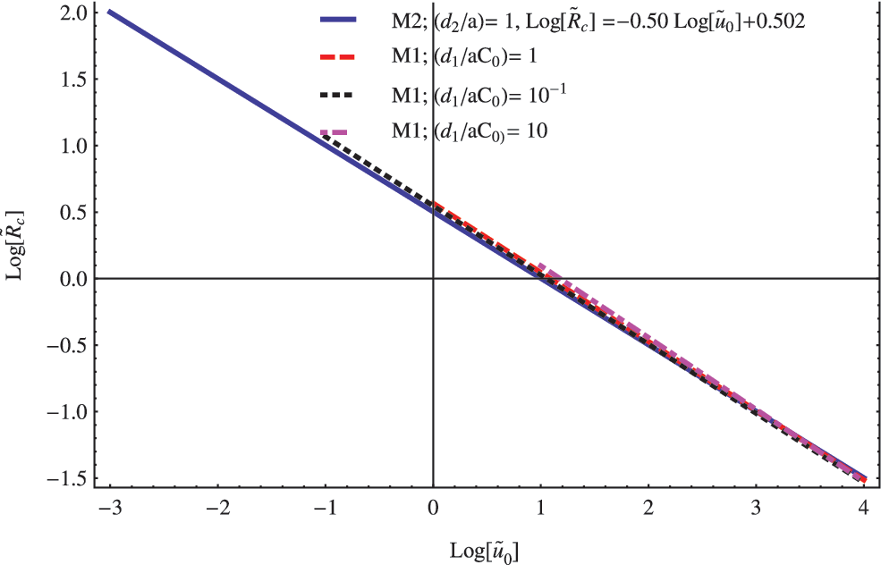
In general, we find that only large-enough vesicles with \documentclass{aastex}\usepackage{amsbsy}\usepackage{amsfonts}\usepackage{amssymb}\usepackage{bm}\usepackage{mathrsfs}\usepackage{pifont}\usepackage{stmaryrd}\usepackage{textcomp}\usepackage{portland, xspace}\usepackage{amsmath, amsxtra}\usepackage{upgreek}\pagestyle{empty}\DeclareMathSizes{10}{9}{7}{6}\begin{document}$$\left( {{{ \widetilde R}_{ \rm{C}}} < \widetilde R} \right)$$ \end{document} are able to support a non-null steady population of the replicator. Also, we find that the value of the critical radius \documentclass{aastex}\usepackage{amsbsy}\usepackage{amsfonts}\usepackage{amssymb}\usepackage{bm}\usepackage{mathrsfs}\usepackage{pifont}\usepackage{stmaryrd}\usepackage{textcomp}\usepackage{portland, xspace}\usepackage{amsmath, amsxtra}\usepackage{upgreek}\pagestyle{empty}\DeclareMathSizes{10}{9}{7}{6}\begin{document}$${ \widetilde R_{ \rm{C}}}$$ \end{document} is similar in the three models and varies approximately as the inverse of the square root of substrate concentration in the medium. Four different correlation functions obtained during these analyses are shown in Fig. 1. The value of the correlation coefficient was greater than (\documentclass{aastex}\usepackage{amsbsy}\usepackage{amsfonts}\usepackage{amssymb}\usepackage{bm}\usepackage{mathrsfs}\usepackage{pifont}\usepackage{stmaryrd}\usepackage{textcomp}\usepackage{portland, xspace}\usepackage{amsmath, amsxtra}\usepackage{upgreek}\pagestyle{empty}\DeclareMathSizes{10}{9}{7}{6}\begin{document}$${r^2} > 0.99$$ \end{document}) in all considered cases.
For both models, the critical radius \documentclass{aastex}\usepackage{amsbsy}\usepackage{amsfonts}\usepackage{amssymb}\usepackage{bm}\usepackage{mathrsfs}\usepackage{pifont}\usepackage{stmaryrd}\usepackage{textcomp}\usepackage{portland, xspace}\usepackage{amsmath, amsxtra}\usepackage{upgreek}\pagestyle{empty}\DeclareMathSizes{10}{9}{7}{6}\begin{document}$${ \widetilde R_{ \rm{C}}} \;$$ \end{document} scales approximately as the inverse of the square root of substrate concentration at the cell boundary.
On the other hand, despite these similarities, there are noticeable asymmetries between the predictions derived from the M1 and M2 models. For instance, whereas the integrated parameter \documentclass{aastex}\usepackage{amsbsy}\usepackage{amsfonts}\usepackage{amssymb}\usepackage{bm}\usepackage{mathrsfs}\usepackage{pifont}\usepackage{stmaryrd}\usepackage{textcomp}\usepackage{portland, xspace}\usepackage{amsmath, amsxtra}\usepackage{upgreek}\pagestyle{empty}\DeclareMathSizes{10}{9}{7}{6}\begin{document}$$\left( { { \frac { { D_1 } } { { D_2 } } } } \right) \left ( { \frac { { { d_2 } } } { a } } \right )$$ \end{document} is not relevant in the value of the critical radius \documentclass{aastex}\usepackage{amsbsy}\usepackage{amsfonts}\usepackage{amssymb}\usepackage{bm}\usepackage{mathrsfs}\usepackage{pifont}\usepackage{stmaryrd}\usepackage{textcomp}\usepackage{portland, xspace}\usepackage{amsmath, amsxtra}\usepackage{upgreek}\pagestyle{empty}\DeclareMathSizes{10}{9}{7}{6}\begin{document}$${ \widetilde R_{ \rm{C}}}$$ \end{document} in the context of the M2 model, this is not the case of the parameter \documentclass{aastex}\usepackage{amsbsy}\usepackage{amsfonts}\usepackage{amssymb}\usepackage{bm}\usepackage{mathrsfs}\usepackage{pifont}\usepackage{stmaryrd}\usepackage{textcomp}\usepackage{portland, xspace}\usepackage{amsmath, amsxtra}\usepackage{upgreek}\pagestyle{empty}\DeclareMathSizes{10}{9}{7}{6}\begin{document}$$\left( { { \frac { { d_1 } } { a \; { C_0 } } } } \right)$$ \end{document} in the context of the M1 model. In this particular case, the ratio \documentclass{aastex}\usepackage{amsbsy}\usepackage{amsfonts}\usepackage{amssymb}\usepackage{bm}\usepackage{mathrsfs}\usepackage{pifont}\usepackage{stmaryrd}\usepackage{textcomp}\usepackage{portland, xspace}\usepackage{amsmath, amsxtra}\usepackage{upgreek}\pagestyle{empty}\DeclareMathSizes{10}{9}{7}{6}\begin{document}$$\left( { { \frac { { d_1 } } { a \; { C_0 } } } } \right)$$ \end{document} determined the lowest bound for the substrate concentration expressed in a nondimensional form. To check the above statement, we rewrite Eq. 6 for \documentclass{aastex}\usepackage{amsbsy}\usepackage{amsfonts}\usepackage{amssymb}\usepackage{bm}\usepackage{mathrsfs}\usepackage{pifont}\usepackage{stmaryrd}\usepackage{textcomp}\usepackage{portland, xspace}\usepackage{amsmath, amsxtra}\usepackage{upgreek}\pagestyle{empty}\DeclareMathSizes{10}{9}{7}{6}\begin{document}$$n = 2$$ \end{document} but considering that \documentclass{aastex}\usepackage{amsbsy}\usepackage{amsfonts}\usepackage{amssymb}\usepackage{bm}\usepackage{mathrsfs}\usepackage{pifont}\usepackage{stmaryrd}\usepackage{textcomp}\usepackage{portland, xspace}\usepackage{amsmath, amsxtra}\usepackage{upgreek}\pagestyle{empty}\DeclareMathSizes{10}{9}{7}{6}\begin{document}$$\widetilde u = \displaystyle { \frac { { { \widetilde u } _r } } { \widetilde r } } = { \frac { { d_1 } } { a \; { C_0 } } } $$ \end{document}. After that, Eq. 6 is simply reduced to\documentclass{aastex}\usepackage{amsbsy}\usepackage{amsfonts}\usepackage{amssymb}\usepackage{bm}\usepackage{mathrsfs}\usepackage{pifont}\usepackage{stmaryrd}\usepackage{textcomp}\usepackage{portland, xspace}\usepackage{amsmath, amsxtra}\usepackage{upgreek}\pagestyle{empty}\DeclareMathSizes{10}{9}{7}{6}\begin{document} \begin{align*}{ \frac { { \partial ^2 } { { \widetilde v } _r } } { \partial { { \widetilde r } ^2 } } } = 0 \tag { 9 } \end{align*} \end{document}
where the solutions are always linear. According to that, it is easy to see that the null solution is the only one that satisfies the boundary conditions expressed in Eqs. 6–7. Once again, we would like to emphasize that the specific choice for the term C0 does not affect our estimations. In the former expressions, the term appears only as a unit correction factor, taking into account that the parameters d1 and d2 are not dimensionally equivalent.
Now, according to the information displayed in Fig. 1, we derive a dimensional expression for the critical radius \documentclass{aastex}\usepackage{amsbsy}\usepackage{amsfonts}\usepackage{amssymb}\usepackage{bm}\usepackage{mathrsfs}\usepackage{pifont}\usepackage{stmaryrd}\usepackage{textcomp}\usepackage{portland, xspace}\usepackage{amsmath, amsxtra}\usepackage{upgreek}\pagestyle{empty}\DeclareMathSizes{10}{9}{7}{6}\begin{document}$${R_{ \rm{C}}}$$ \end{document}. By combining the scale transformation (last equation in 4) and the expression for \documentclass{aastex}\usepackage{amsbsy}\usepackage{amsfonts}\usepackage{amssymb}\usepackage{bm}\usepackage{mathrsfs}\usepackage{pifont}\usepackage{stmaryrd}\usepackage{textcomp}\usepackage{portland, xspace}\usepackage{amsmath, amsxtra}\usepackage{upgreek}\pagestyle{empty}\DeclareMathSizes{10}{9}{7}{6}\begin{document}$${ \widetilde R_{ \rm{C}}}$$ \end{document} obtained for the M2 model, it is possible to rewrite the expression of the critical radius \documentclass{aastex}\usepackage{amsbsy}\usepackage{amsfonts}\usepackage{amssymb}\usepackage{bm}\usepackage{mathrsfs}\usepackage{pifont}\usepackage{stmaryrd}\usepackage{textcomp}\usepackage{portland, xspace}\usepackage{amsmath, amsxtra}\usepackage{upgreek}\pagestyle{empty}\DeclareMathSizes{10}{9}{7}{6}\begin{document}$${R_{ \rm{C}}} \;$$ \end{document} expressed in the original dimensional system as follows:\documentclass{aastex}\usepackage{amsbsy}\usepackage{amsfonts}\usepackage{amssymb}\usepackage{bm}\usepackage{mathrsfs}\usepackage{pifont}\usepackage{stmaryrd}\usepackage{textcomp}\usepackage{portland, xspace}\usepackage{amsmath, amsxtra}\usepackage{upgreek}\pagestyle{empty}\DeclareMathSizes{10}{9}{7}{6}\begin{document} \begin{align*}{ R_ { \rm { C } } } = 3.181 \; { \left( { { \frac { { D_2 } } { a \; { u_0 } \; } } } \right) ^ { \frac { 1 } { 2 } } } \tag { 10 } \end{align*} \end{document}
This last expression shows explicitly the three main factors \documentclass{aastex}\usepackage{amsbsy}\usepackage{amsfonts}\usepackage{amssymb}\usepackage{bm}\usepackage{mathrsfs}\usepackage{pifont}\usepackage{stmaryrd}\usepackage{textcomp}\usepackage{portland, xspace}\usepackage{amsmath, amsxtra}\usepackage{upgreek}\pagestyle{empty}\DeclareMathSizes{10}{9}{7}{6}\begin{document}$$\left\{ {{D_2} , a , {u_0}} \right\} $$ \end{document} that determine the habitability of a vesicle in the context of the M2 model. Furthermore, we do not find differences when the expression is derived directly from the F-K equation, with the exception of a slightly lower value in the numerical factor (3.15 instead of 3.18), probably as a consequence of numerical uncertainties. In this sense, both models are equivalent without evidencing any dependence on the additional parameters included in our model. Furthermore, the former expression (Eq. 10) is also an acceptable approximation in the case of the M1 model (see Fig. 1 for details). The exponents, in this case, were slightly different, varying from 0.52 to 0.54 instead of 0.5 obtained for the M2 model. However, as we have already discussed, in this case the range of permissible substrate concentrations is restricted to be greater than \documentclass{aastex}\usepackage{amsbsy}\usepackage{amsfonts}\usepackage{amssymb}\usepackage{bm}\usepackage{mathrsfs}\usepackage{pifont}\usepackage{stmaryrd}\usepackage{textcomp}\usepackage{portland, xspace}\usepackage{amsmath, amsxtra}\usepackage{upgreek}\pagestyle{empty}\DeclareMathSizes{10}{9}{7}{6}\begin{document}$$\left( { { u_0 } > { u_ { { \rm { min } } } } = { \frac { { d_1 } } { a \; } } } \right)$$ \end{document}. This is equivalent to the existence of a maximum critical radius of the vesicle \documentclass{aastex}\usepackage{amsbsy}\usepackage{amsfonts}\usepackage{amssymb}\usepackage{bm}\usepackage{mathrsfs}\usepackage{pifont}\usepackage{stmaryrd}\usepackage{textcomp}\usepackage{portland, xspace}\usepackage{amsmath, amsxtra}\usepackage{upgreek}\pagestyle{empty}\DeclareMathSizes{10}{9}{7}{6}\begin{document}$${R_{{ \rm{Cmax}}}}$$ \end{document} determined by the ratio between the diffusion constant of the replicator D2 and the first-order rate constant of lethality d1,\documentclass{aastex}\usepackage{amsbsy}\usepackage{amsfonts}\usepackage{amssymb}\usepackage{bm}\usepackage{mathrsfs}\usepackage{pifont}\usepackage{stmaryrd}\usepackage{textcomp}\usepackage{portland, xspace}\usepackage{amsmath, amsxtra}\usepackage{upgreek}\pagestyle{empty}\DeclareMathSizes{10}{9}{7}{6}\begin{document} \begin{align*}{ R_ { { \rm { Cmax } } } } \approx 3.181 \; { \left( { { \frac { { D_2 } } { a \; { u_ { { \rm { min } } } } \; } } } \right) ^ { \frac { 1 } { 2 } } } = 3.181 \; { \left( { { \frac { { D_2 } } { { d_1 } \; } } } \right) ^ { \frac { 1 } { 2 } } } \tag { 11 } \end{align*} \end{document}
According to Eq. 11, habitable vesicles for replicators with linear decay are constrained to have \documentclass{aastex}\usepackage{amsbsy}\usepackage{amsfonts}\usepackage{amssymb}\usepackage{bm}\usepackage{mathrsfs}\usepackage{pifont}\usepackage{stmaryrd}\usepackage{textcomp}\usepackage{portland, xspace}\usepackage{amsmath, amsxtra}\usepackage{upgreek}\pagestyle{empty}\DeclareMathSizes{10}{9}{7}{6}\begin{document}$$\left( {{R_{ \rm{C}}} < {R_{{ \rm{Cmax}}}}} \right)$$ \end{document}. Such a feature is unique in the context of the M1 model and does not appear in the other two models considered here.
Now, we discuss the relevance of the parameters included in the \documentclass{aastex}\usepackage{amsbsy}\usepackage{amsfonts}\usepackage{amssymb}\usepackage{bm}\usepackage{mathrsfs}\usepackage{pifont}\usepackage{stmaryrd}\usepackage{textcomp}\usepackage{portland, xspace}\usepackage{amsmath, amsxtra}\usepackage{upgreek}\pagestyle{empty}\DeclareMathSizes{10}{9}{7}{6}\begin{document}$${R_{ \rm{C}}}$$ \end{document} expression (Eq. 10). In the first place, we find that the critical radius decreases as the ability of the replicator to diffuse also decreases. In general, the diffusion constant D2 diminishes as the molecular weight of the replicator increases depending also on its chemical nature. Typical biological values for the diffusion constant range from \documentclass{aastex}\usepackage{amsbsy}\usepackage{amsfonts}\usepackage{amssymb}\usepackage{bm}\usepackage{mathrsfs}\usepackage{pifont}\usepackage{stmaryrd}\usepackage{textcomp}\usepackage{portland, xspace}\usepackage{amsmath, amsxtra}\usepackage{upgreek}\pagestyle{empty}\DeclareMathSizes{10}{9}{7}{6}\begin{document}$${10^{ - 9}} \;{{ \rm{m}}^2} \;{{ \rm{s}}^{ - 1}}$$ \end{document} to \documentclass{aastex}\usepackage{amsbsy}\usepackage{amsfonts}\usepackage{amssymb}\usepackage{bm}\usepackage{mathrsfs}\usepackage{pifont}\usepackage{stmaryrd}\usepackage{textcomp}\usepackage{portland, xspace}\usepackage{amsmath, amsxtra}\usepackage{upgreek}\pagestyle{empty}\DeclareMathSizes{10}{9}{7}{6}\begin{document}$${10^{ - 11}}{ \rm{ \;}}{{ \rm{m}}^2} \;{{ \rm{s}}^{ - 1}}$$ \end{document}, being lower in the cases of very large biomolecules such as proteins or nucleic acids. However, even when we do not know what kind of replicators were successful in the environments of early Earth, it makes sense to search in the set of organic compounds with light or middle molecular weights (King, 1982, 1986), respectively. These types of replicators could have better chances of success in a chemical environment of limited complexity.
In the second place, we find that the availability of substrate in the medium is a key factor in determining the critical radius \documentclass{aastex}\usepackage{amsbsy}\usepackage{amsfonts}\usepackage{amssymb}\usepackage{bm}\usepackage{mathrsfs}\usepackage{pifont}\usepackage{stmaryrd}\usepackage{textcomp}\usepackage{portland, xspace}\usepackage{amsmath, amsxtra}\usepackage{upgreek}\pagestyle{empty}\DeclareMathSizes{10}{9}{7}{6}\begin{document}$${ \widetilde R_{ \rm{C}}}$$ \end{document} under which the replicator population is not viable. From this point of view, the potential habitability of small vesicles to harbor a replicator species could be seriously limited in a medium where the nutrient content is rather low. According to our results, only vesicles with enough size could be able to support a steady population of replicator under such conditions. Furthermore, the problem of the nutrient shortage is even more drastic in the context of the M1 model. In this case, the habitability is only possible when the concentration of substrate exceeds a well-determined threshold. These kinds of dependencies could be crucial for the ulterior destiny of life on Earth. The availability of organic material in early Earth rises as a problematic issue in the most accepted scenarios for the origin of life. The role of the atmosphere as a source of organic material appears to be rather limited (Trainer, 2013). However, we cannot discard at all the existence of potential microhabitats where the content of nutrients could reach high levels. Probably such conditions hold in the environment of some hydrothermal vents (Martin et al.,2008; Ehrenfreund et al.,2011), in submerged caves, or simply in small cavities formed in rock in marine environments (Hanczyc et al.,2007). In the same way, we cannot discard the possibility of recycling the waste products in the external medium driven by a solar or geothermal energy source. This kind of process may contribute, at least to some extent, to regenerate the levels of substrate concentration in the medium. The role of recycling as an effective way to preserve organic matter in the origin of life was envisioned early on by King (1982, 1986).
On the other hand, we must take into account another problematic question. Habitable vesicles must increase their size when the substrate concentration in the medium decreases; however, the increases of the vesicle surface demand an increment of the organic matter needed to make the vesicle itself. We must take into account that in spherical vesicles the surface increases as \documentclass{aastex}\usepackage{amsbsy}\usepackage{amsfonts}\usepackage{amssymb}\usepackage{bm}\usepackage{mathrsfs}\usepackage{pifont}\usepackage{stmaryrd}\usepackage{textcomp}\usepackage{portland, xspace}\usepackage{amsmath, amsxtra}\usepackage{upgreek}\pagestyle{empty}\DeclareMathSizes{10}{9}{7}{6}\begin{document}$${R^2}$$ \end{document}. It is probably the case that a compromise is involved between both factors. Regardless, the possibilities for establishing steady-state populations of replicators inside vesicles under these conditions are rather small. The existence of active transport across the membrane could help circumvent this limitation. However, active transport appears to be a complex strategy developed during biological evolution to deal with the scarcity of nutrients in the medium. Consequently, the existence of such a mechanism in the incipient forms of life driven basically by diffusion is highly improbable.
Finally, we find that the overall process also depends on the value of the reproduction rate constant a. As the replication rate increases, the critical radius is reduced, which favors the habitability of smaller vesicles. From the molecular point of view, the value of this constant expresses the efficiency of the interaction between both species, the replicator on the substrate in the process to make copies of itself. The typical values of a are system dependent, being conditioned, in most cases, by steric and energetic requirements. In principle, these values could change as a consequence of stochastic fluctuations in the environment (Mulkidjanian et al.,2003; Lincoln and Joyce, 2009; Martín and Horvath, 2013; Robertson and Joyce, 2014). This is particularly important when the replicator's species are able to evolve as is the case of nucleic acids: DNA and especially RNA (Lincoln and Joyce, 2009; Robertson and Joyce, 2014). In these cases, the paradigm of survival of the fittest, the essence of Darwinian evolution, enhances the potential to colonize smaller vesicles over the course of time.
On the other hand, the existence of a critical radius reinforces the idea of considering the phenomenon of life from a system perspective (Ruiz-Mirazo et al.,2014; de la Escosura et al.,2015) rather than the outcome of molecular replication processes in a relatively rich chemical scenario. Note that the success or failure of a particular family of replicator inside a vesicle is not totally determined by its own potential but also for the vesicle size. In this case, the lack of plasticity is strongly linked with the impossibility of the system to compensate for the continued degradation imposed to the replicators outside the vesicle. In the context of the work of Piedrafita et al. (2012), Eq. 10 provides, under a very particular set of conditions, the theoretical bounds where the self-suffocation of the replication mechanisms inside the vesicle arises. However, in this case the self-suffocation is driven not only by a limited source of nutrients but also by the harmful environmental influence on the products. Similar changes of plasticity are also discussed in other works (Piedrafita et al.,2010, 2017); however, in these cases the changes are more linked with the choice and robustness of the proto-metabolic networks considered during these studies.
Additionally, there are other elements that could be connected with the former scenarios. For instance, even when we are not considering explicitly a coupling between the membrane and the inner metabolism (see for instance Piedrafita et al. [2017] as an example of such coupling in a milder environment), an inhabited vesicle may increase its size as a consequence of the osmotic gradient due to the accumulation of end products with low permeability. Probably, this situation is applicable to the M2 model where the form of the decay term \documentclass{aastex}\usepackage{amsbsy}\usepackage{amsfonts}\usepackage{amssymb}\usepackage{bm}\usepackage{mathrsfs}\usepackage{pifont}\usepackage{stmaryrd}\usepackage{textcomp}\usepackage{portland, xspace}\usepackage{amsmath, amsxtra}\usepackage{upgreek}\pagestyle{empty}\DeclareMathSizes{10}{9}{7}{6}\begin{document}$$( - {d_2} \;{v^2} \; )$$ \end{document} implies the formation of a new species v2 with higher molecular mass as a consequence of the reaction between two molecules of the replicator.
Furthermore, we also explore in a very preliminary way how the subsequent polymerization of this species to form dimers, trimers, and so on might affect the \documentclass{aastex}\usepackage{amsbsy}\usepackage{amsfonts}\usepackage{amssymb}\usepackage{bm}\usepackage{mathrsfs}\usepackage{pifont}\usepackage{stmaryrd}\usepackage{textcomp}\usepackage{portland, xspace}\usepackage{amsmath, amsxtra}\usepackage{upgreek}\pagestyle{empty}\DeclareMathSizes{10}{9}{7}{6}\begin{document}$${R_{ \rm{C}}}$$ \end{document} value. To this end, we included the reaction diffusion of the polymeric species in the original system (Eqs. 1–2):\documentclass{aastex}\usepackage{amsbsy}\usepackage{amsfonts}\usepackage{amssymb}\usepackage{bm}\usepackage{mathrsfs}\usepackage{pifont}\usepackage{stmaryrd}\usepackage{textcomp}\usepackage{portland, xspace}\usepackage{amsmath, amsxtra}\usepackage{upgreek}\pagestyle{empty}\DeclareMathSizes{10}{9}{7}{6}\begin{document} \begin{align*}{ \frac { \partial { v_2 } } { \partial t } } = { D_3 } \left( { { \frac { { \partial ^2 } { v_2 } } { \partial { r^2 } } } + \frac { 2 } { r } { \frac { \partial { v_2 } } { \partial r } } } \right) + { d_2 } { v^2 } - { d_3 } { v_2 } v = 0 \tag { 12 } \end{align*} \end{document}
where D3 is the corresponding diffusion coefficient and d2 and d3 are the step-growth rate coefficients for dimer and trimer production, respectively. In this case, we considered only the production of dimers v2, even when the lost term \documentclass{aastex}\usepackage{amsbsy}\usepackage{amsfonts}\usepackage{amssymb}\usepackage{bm}\usepackage{mathrsfs}\usepackage{pifont}\usepackage{stmaryrd}\usepackage{textcomp}\usepackage{portland, xspace}\usepackage{amsmath, amsxtra}\usepackage{upgreek}\pagestyle{empty}\DeclareMathSizes{10}{9}{7}{6}\begin{document}$$( - {v_{2 \;}}v )$$ \end{document} in the dynamics implicitly included the trimer production. Additionally, we assumed that \documentclass{aastex}\usepackage{amsbsy}\usepackage{amsfonts}\usepackage{amssymb}\usepackage{bm}\usepackage{mathrsfs}\usepackage{pifont}\usepackage{stmaryrd}\usepackage{textcomp}\usepackage{portland, xspace}\usepackage{amsmath, amsxtra}\usepackage{upgreek}\pagestyle{empty}\DeclareMathSizes{10}{9}{7}{6}\begin{document}$$( {d_2} = {d_3} )$$ \end{document} and the diffusion coefficient for the dimer D3 is similar to that used for the other two species.
However, the numerical exploration of the system including explicitly the possibility of subsequent polymerization of the replicator (Eq. 12) did not alter our previous estimations of the \documentclass{aastex}\usepackage{amsbsy}\usepackage{amsfonts}\usepackage{amssymb}\usepackage{bm}\usepackage{mathrsfs}\usepackage{pifont}\usepackage{stmaryrd}\usepackage{textcomp}\usepackage{portland, xspace}\usepackage{amsmath, amsxtra}\usepackage{upgreek}\pagestyle{empty}\DeclareMathSizes{10}{9}{7}{6}\begin{document}$${R_{ \rm{C}}}$$ \end{document} value. In this sense, the potential to increase molecular complexity and self-organization from the elemental replicator species in our scenario appears to be constrained to the same expression for the \documentclass{aastex}\usepackage{amsbsy}\usepackage{amsfonts}\usepackage{amssymb}\usepackage{bm}\usepackage{mathrsfs}\usepackage{pifont}\usepackage{stmaryrd}\usepackage{textcomp}\usepackage{portland, xspace}\usepackage{amsmath, amsxtra}\usepackage{upgreek}\pagestyle{empty}\DeclareMathSizes{10}{9}{7}{6}\begin{document}$${R_{ \rm{C}}}$$ \end{document}. However, a better comprehension of these processes may require the development of a more exhaustive study. For instance, the progressive increase of the molecular weight of some polymeric species (macromolecules) together with a gradual decrease in their concentrations inside the vesicle may require the use of a stochastic approach rather than the deterministic one used during this work.
In a more practical sense, Eqs. 10 and 11 also give us the possibility to explore the kinetic requirements of a replicator adjusted to the conditions of our models. For instance, consider the radius of a typical vesicle of about \documentclass{aastex}\usepackage{amsbsy}\usepackage{amsfonts}\usepackage{amssymb}\usepackage{bm}\usepackage{mathrsfs}\usepackage{pifont}\usepackage{stmaryrd}\usepackage{textcomp}\usepackage{portland, xspace}\usepackage{amsmath, amsxtra}\usepackage{upgreek}\pagestyle{empty}\DeclareMathSizes{10}{9}{7}{6}\begin{document}$$R = 1 \;{{ \mu {\rm m}}}$$ \end{document} as an estimation of the \documentclass{aastex}\usepackage{amsbsy}\usepackage{amsfonts}\usepackage{amssymb}\usepackage{bm}\usepackage{mathrsfs}\usepackage{pifont}\usepackage{stmaryrd}\usepackage{textcomp}\usepackage{portland, xspace}\usepackage{amsmath, amsxtra}\usepackage{upgreek}\pagestyle{empty}\DeclareMathSizes{10}{9}{7}{6}\begin{document}$${R_{ \rm{C}}}$$ \end{document} value, a diffusion constant of \documentclass{aastex}\usepackage{amsbsy}\usepackage{amsfonts}\usepackage{amssymb}\usepackage{bm}\usepackage{mathrsfs}\usepackage{pifont}\usepackage{stmaryrd}\usepackage{textcomp}\usepackage{portland, xspace}\usepackage{amsmath, amsxtra}\usepackage{upgreek}\pagestyle{empty}\DeclareMathSizes{10}{9}{7}{6}\begin{document}$${D_2} = {10^{ - 11}} \;{{ \rm{m}}^2} \;{{ \rm{s}}^{ - 1}}$$ \end{document}, and a substrate concentration of the order \documentclass{aastex}\usepackage{amsbsy}\usepackage{amsfonts}\usepackage{amssymb}\usepackage{bm}\usepackage{mathrsfs}\usepackage{pifont}\usepackage{stmaryrd}\usepackage{textcomp}\usepackage{portland, xspace}\usepackage{amsmath, amsxtra}\usepackage{upgreek}\pagestyle{empty}\DeclareMathSizes{10}{9}{7}{6}\begin{document}$${u_0} = 1 \;{\hbox{u {\rm mol d}}}{{ \rm{m}}^{ - 3}}$$ \end{document}. Solving Eq. 10 for the reproduction parameter and evaluating it, we find an extremely high value for the reproduction parameter \documentclass{aastex}\usepackage{amsbsy}\usepackage{amsfonts}\usepackage{amssymb}\usepackage{bm}\usepackage{mathrsfs}\usepackage{pifont}\usepackage{stmaryrd}\usepackage{textcomp}\usepackage{portland, xspace}\usepackage{amsmath, amsxtra}\usepackage{upgreek}\pagestyle{empty}\DeclareMathSizes{10}{9}{7}{6}\begin{document}$$\left( {a \approx {{10}^8} \;{ \rm{d}}{{ \rm{m}}^3}{ \rm{ \;mo}}{{ \rm{l}}^{ - 1}}{ \rm{ \;}}{{ \rm{s}}^{ - 1}}} \right)$$ \end{document}, just in the diffusion-controlled limit for a chemical reaction \documentclass{aastex}\usepackage{amsbsy}\usepackage{amsfonts}\usepackage{amssymb}\usepackage{bm}\usepackage{mathrsfs}\usepackage{pifont}\usepackage{stmaryrd}\usepackage{textcomp}\usepackage{portland, xspace}\usepackage{amsmath, amsxtra}\usepackage{upgreek}\pagestyle{empty}\DeclareMathSizes{10}{9}{7}{6}\begin{document}$$( {10^8} \;{ \rm{to}} \;{10^9} \;{ \rm{d}}{{ \rm{m}}^3} \;{ \rm{mo}}{{ \rm{l}}^{ - 1}}{ \rm{ \;}}{{ \rm{s}}^{ - 1}} )$$ \end{document}. Fulfilling such a demanding biotic chemistry. However, considering a larger vesicle of about \documentclass{aastex}\usepackage{amsbsy}\usepackage{amsfonts}\usepackage{amssymb}\usepackage{bm}\usepackage{mathrsfs}\usepackage{pifont}\usepackage{stmaryrd}\usepackage{textcomp}\usepackage{portland, xspace}\usepackage{amsmath, amsxtra}\usepackage{upgreek}\pagestyle{empty}\DeclareMathSizes{10}{9}{7}{6}\begin{document}$$R = 10 \;{{ \mu {\rm m}}}$$ \end{document} and a substrate concentration of \documentclass{aastex}\usepackage{amsbsy}\usepackage{amsfonts}\usepackage{amssymb}\usepackage{bm}\usepackage{mathrsfs}\usepackage{pifont}\usepackage{stmaryrd}\usepackage{textcomp}\usepackage{portland, xspace}\usepackage{amsmath, amsxtra}\usepackage{upgreek}\pagestyle{empty}\DeclareMathSizes{10}{9}{7}{6}\begin{document}$${u_0} = 10 \;{{ \mu\hbox{mol d}}}{{ \rm{m}}^{ - 3}}$$ \end{document}, we find that \documentclass{aastex}\usepackage{amsbsy}\usepackage{amsfonts}\usepackage{amssymb}\usepackage{bm}\usepackage{mathrsfs}\usepackage{pifont}\usepackage{stmaryrd}\usepackage{textcomp}\usepackage{portland, xspace}\usepackage{amsmath, amsxtra}\usepackage{upgreek}\pagestyle{empty}\DeclareMathSizes{10}{9}{7}{6}\begin{document}$$a \approx {10^5} \;{ \rm{d}}{{ \rm{m}}^3} \;{ \rm{mo}}{{ \rm{l}}^{ - 1}}{ \rm{ \;}}{{ \rm{s}}^{ - 1}}$$ \end{document}, a value that coincides with the average of the catalytic efficiencies displayed by contemporary enzymes (Bar-Even et al., 2011).
3.2. Factors affecting the population of replicators
According to the concept of kinetic stability introduced by Pross (Pross, 2005a, 2011; Pross and Khodorkovsky, 2004), the size of replicator population at steady state could be considered as a direct measure of the robustness of the system. Here, we discuss briefly how the different parameters influence the population according to the different models, even when some of them do not have a direct impact on the \documentclass{aastex}\usepackage{amsbsy}\usepackage{amsfonts}\usepackage{amssymb}\usepackage{bm}\usepackage{mathrsfs}\usepackage{pifont}\usepackage{stmaryrd}\usepackage{textcomp}\usepackage{portland, xspace}\usepackage{amsmath, amsxtra}\usepackage{upgreek}\pagestyle{empty}\DeclareMathSizes{10}{9}{7}{6}\begin{document}$${R_{ \rm{C}}}$$ \end{document} value. In this case, as both the dimensional and nondimensional concentrations scale linearly, most of the analyses in this section considered dimensionless concentrations, with the exception of one case where its use could be confusing for the reader.
3.2.1. The size of the cell
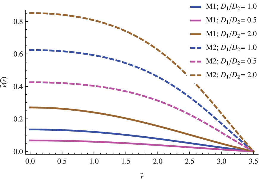
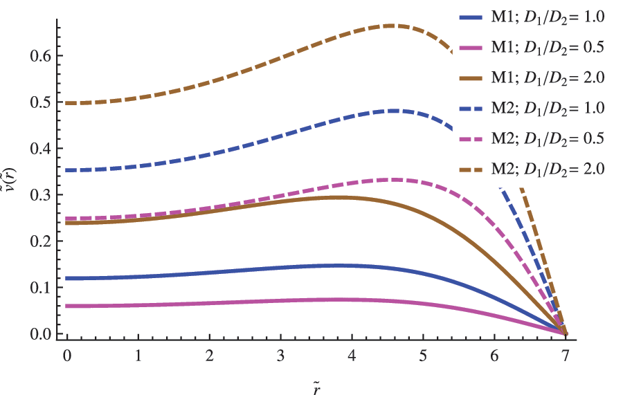
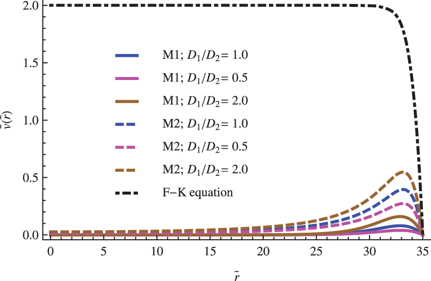
The size of the vesicle R becomes an important parameter when modeling the replicator's population inside the vesicle. In general, and independent of the model used in the analysis, as the size of the vesicle increases, noticeable changes occur in the radial profile of concentrations. For vesicles with radius R close to the critical radius \documentclass{aastex}\usepackage{amsbsy}\usepackage{amsfonts}\usepackage{amssymb}\usepackage{bm}\usepackage{mathrsfs}\usepackage{pifont}\usepackage{stmaryrd}\usepackage{textcomp}\usepackage{portland, xspace}\usepackage{amsmath, amsxtra}\usepackage{upgreek}\pagestyle{empty}\DeclareMathSizes{10}{9}{7}{6}\begin{document}$${R_{ \rm{C}}}$$ \end{document}, the replicator concentrations exhibit a maximum in the central region of the vesicle (see Fig. 2). With the exception of the behavior obtained from the F-K equation, the maximum is shifted to the exterior region as the radius increases to larger values, which decreases the concentration in the central region (see Figs. 3 and 4). For the largest cells, \documentclass{aastex}\usepackage{amsbsy}\usepackage{amsfonts}\usepackage{amssymb}\usepackage{bm}\usepackage{mathrsfs}\usepackage{pifont}\usepackage{stmaryrd}\usepackage{textcomp}\usepackage{portland, xspace}\usepackage{amsmath, amsxtra}\usepackage{upgreek}\pagestyle{empty}\DeclareMathSizes{10}{9}{7}{6}\begin{document}$${R_{ \rm{C}}} \;\gg\, R$$ \end{document}, the population peaks close to the cell boundary (see Fig. 4), whereas the concentration in the center becomes negligible, which confirms a limited diffusion and a prevalence of a kinetic control determining the overall process. A similar criterion was used by Catling et al. (2005) and Newton-Harvey (1928) to infer the size of the largest aerobic cell as a function of the oxygen levels in the atmosphere. In that case, the availably of a substrate (oxygen) near the center of the cell becomes the limiting condition, a plausible restriction taking into account that this species provides the energetic requirements to support the cellular machinery functioning.
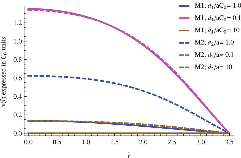
The influence of the \documentclass{aastex}\usepackage{amsbsy}\usepackage{amsfonts}\usepackage{amssymb}\usepackage{bm}\usepackage{mathrsfs}\usepackage{pifont}\usepackage{stmaryrd}\usepackage{textcomp}\usepackage{portland, xspace}\usepackage{amsmath, amsxtra}\usepackage{upgreek}\pagestyle{empty}\DeclareMathSizes{10}{9}{7}{6}\begin{document}$$\left( { { \frac { { D_1 } } { { D_2 } } } } \right)$$ \end{document} ratio in the nondimensional concentration profile for the replicator. The other parameters were set to \documentclass{aastex}\usepackage{amsbsy}\usepackage{amsfonts}\usepackage{amssymb}\usepackage{bm}\usepackage{mathrsfs}\usepackage{pifont}\usepackage{stmaryrd}\usepackage{textcomp}\usepackage{portland, xspace}\usepackage{amsmath, amsxtra}\usepackage{upgreek}\pagestyle{empty}\DeclareMathSizes{10}{9}{7}{6}\begin{document}$$\left\{ { \widetilde R = 3.5; \; \left( { { \frac { { d_n } } { a \; { C_0 } ^ { 2 - n } } } } \right) = 1; { \hbox { } } { { \widetilde u } _0 } = 2 } \right\} $$ \end{document}.
The influence of the \documentclass{aastex}\usepackage{amsbsy}\usepackage{amsfonts}\usepackage{amssymb}\usepackage{bm}\usepackage{mathrsfs}\usepackage{pifont}\usepackage{stmaryrd}\usepackage{textcomp}\usepackage{portland, xspace}\usepackage{amsmath, amsxtra}\usepackage{upgreek}\pagestyle{empty}\DeclareMathSizes{10}{9}{7}{6}\begin{document}$$\left( { { \frac { { D_1 } } { { D_2 } } } } \right)$$ \end{document} ratio in the nondimensional concentration profile for the replicator. The other parameters were set to \documentclass{aastex}\usepackage{amsbsy}\usepackage{amsfonts}\usepackage{amssymb}\usepackage{bm}\usepackage{mathrsfs}\usepackage{pifont}\usepackage{stmaryrd}\usepackage{textcomp}\usepackage{portland, xspace}\usepackage{amsmath, amsxtra}\usepackage{upgreek}\pagestyle{empty}\DeclareMathSizes{10}{9}{7}{6}\begin{document}$$\left\{ { \widetilde R = 7; \; \left( { { \frac { { d_n } } { a \; { C_0 } ^ { 2 - n } } } } \right) = 1; { \hbox { } } { { \widetilde u } _0 } = 2 } \right\} $$ \end{document}.
The influence of the \documentclass{aastex}\usepackage{amsbsy}\usepackage{amsfonts}\usepackage{amssymb}\usepackage{bm}\usepackage{mathrsfs}\usepackage{pifont}\usepackage{stmaryrd}\usepackage{textcomp}\usepackage{portland, xspace}\usepackage{amsmath, amsxtra}\usepackage{upgreek}\pagestyle{empty}\DeclareMathSizes{10}{9}{7}{6}\begin{document}$$\left( { { \frac { { D_1 } } { { D_2 } } } } \right)$$ \end{document} ratio in the nondimensional concentration profile for the replicator. The other parameters were set to \documentclass{aastex}\usepackage{amsbsy}\usepackage{amsfonts}\usepackage{amssymb}\usepackage{bm}\usepackage{mathrsfs}\usepackage{pifont}\usepackage{stmaryrd}\usepackage{textcomp}\usepackage{portland, xspace}\usepackage{amsmath, amsxtra}\usepackage{upgreek}\pagestyle{empty}\DeclareMathSizes{10}{9}{7}{6}\begin{document}$$\left\{ { \widetilde R = 35; \; \left( { { \frac { { d_n } } { a \; { C_0 } ^ { 2 - n } } } } \right) = 1; { \hbox { } } { { \tilde u } _0 } = 2 } \right\} $$ \end{document}.
Additionally, we also find that the mean concentration of the replicator in the vesicle changes as a function of the vesicle radius. We find the existence of an optimum volume of the vesicle, where the mean value of the replicator concentration reaches a maximum. For instance, for the M2 model and considering that all terms are normalized \documentclass{aastex}\usepackage{amsbsy}\usepackage{amsfonts}\usepackage{amssymb}\usepackage{bm}\usepackage{mathrsfs}\usepackage{pifont}\usepackage{stmaryrd}\usepackage{textcomp}\usepackage{portland, xspace}\usepackage{amsmath, amsxtra}\usepackage{upgreek}\pagestyle{empty}\DeclareMathSizes{10}{9}{7}{6}\begin{document}$$\left\{ { \left( { { \frac { { D_1 } } { { D_2 } } } } \right) = \left( { \frac { d } { a } } \right) = { u_0 } = 1 } \right\} $$ \end{document}, the optimum volume of the vesicle takes place at \documentclass{aastex}\usepackage{amsbsy}\usepackage{amsfonts}\usepackage{amssymb}\usepackage{bm}\usepackage{mathrsfs}\usepackage{pifont}\usepackage{stmaryrd}\usepackage{textcomp}\usepackage{portland, xspace}\usepackage{amsmath, amsxtra}\usepackage{upgreek}\pagestyle{empty}\DeclareMathSizes{10}{9}{7}{6}\begin{document}$$\widetilde R{ \;_{{ \rm{opt}}}} \approx 3{ \widetilde R_{ \rm{C}}}$$ \end{document} reaching the mean concentration, a value that is approximately 4 times greater than the same value estimated at \documentclass{aastex}\usepackage{amsbsy}\usepackage{amsfonts}\usepackage{amssymb}\usepackage{bm}\usepackage{mathrsfs}\usepackage{pifont}\usepackage{stmaryrd}\usepackage{textcomp}\usepackage{portland, xspace}\usepackage{amsmath, amsxtra}\usepackage{upgreek}\pagestyle{empty}\DeclareMathSizes{10}{9}{7}{6}\begin{document}$${ \widetilde R_{ \rm{C}}}$$ \end{document}. For a larger radius, the mean values fall asymptotically, which confirms that the replicator population is diluted in a greater volume.
Figures 2–4 also show a systematic difference in the estimations from M1 and M2 models. In all previous cases, the M2 model estimates larger replicator populations than the M1 model. However, this tendency remains only when the concentration of the substrate in the medium is rather low (\documentclass{aastex}\usepackage{amsbsy}\usepackage{amsfonts}\usepackage{amssymb}\usepackage{bm}\usepackage{mathrsfs}\usepackage{pifont}\usepackage{stmaryrd}\usepackage{textcomp}\usepackage{portland, xspace}\usepackage{amsmath, amsxtra}\usepackage{upgreek}\pagestyle{empty}\DeclareMathSizes{10}{9}{7}{6}\begin{document}$${ \widetilde u_0} = 2$$ \end{document} in this parameterization). More details about the impact of the substrate concentration for both models will be discussed in the next sections.
On the other hand, a very different behavior is indicated by the concentration profiles derived from the F-K equation (see Fig. 4). In all studied cases, the F-K equation overestimates the levels of replicator population inside the vesicle. The differences between these estimations increase as the cell radius becomes greater. We find that, for vesicles with a radius comparable with \documentclass{aastex}\usepackage{amsbsy}\usepackage{amsfonts}\usepackage{amssymb}\usepackage{bm}\usepackage{mathrsfs}\usepackage{pifont}\usepackage{stmaryrd}\usepackage{textcomp}\usepackage{portland, xspace}\usepackage{amsmath, amsxtra}\usepackage{upgreek}\pagestyle{empty}\DeclareMathSizes{10}{9}{7}{6}\begin{document}$${R_{ \rm{C}}}$$ \end{document}, both profiles exhibit the same tendency. However, contrary to our model, the profile derived from the F-K equation tends to saturate for larger vesicles that show unexpected high values of the replicator concentration in the central region of the vesicle (see Fig. 4). Such a tendency is a clear consequence of the unrealistic assumption of an infinite diffusion rate, a limitation that becomes more remarkable as the size of the vesicles increases (\documentclass{aastex}\usepackage{amsbsy}\usepackage{amsfonts}\usepackage{amssymb}\usepackage{bm}\usepackage{mathrsfs}\usepackage{pifont}\usepackage{stmaryrd}\usepackage{textcomp}\usepackage{portland, xspace}\usepackage{amsmath, amsxtra}\usepackage{upgreek}\pagestyle{empty}\DeclareMathSizes{10}{9}{7}{6}\begin{document}$${R_{ \rm{C}}}\, \gg\, R$$ \end{document}).
3.2.2. Differences in the ability to diffuse between substrate and replicator
Diffusive differences between both species are codified in the first factor \documentclass{aastex}\usepackage{amsbsy}\usepackage{amsfonts}\usepackage{amssymb}\usepackage{bm}\usepackage{mathrsfs}\usepackage{pifont}\usepackage{stmaryrd}\usepackage{textcomp}\usepackage{portland, xspace}\usepackage{amsmath, amsxtra}\usepackage{upgreek}\pagestyle{empty}\DeclareMathSizes{10}{9}{7}{6}\begin{document}$$\left( { { \frac { { D_1 } } { { D_2 } } } } \right)$$ \end{document} of Eq. 4. If we assume that the substrate and replicator share the same chemical nature and similar molecular weights, it makes sense to consider approximate values close to the unity for the former ratio \documentclass{aastex}\usepackage{amsbsy}\usepackage{amsfonts}\usepackage{amssymb}\usepackage{bm}\usepackage{mathrsfs}\usepackage{pifont}\usepackage{stmaryrd}\usepackage{textcomp}\usepackage{portland, xspace}\usepackage{amsmath, amsxtra}\usepackage{upgreek}\pagestyle{empty}\DeclareMathSizes{10}{9}{7}{6}\begin{document}$$\left( { { \frac { { D_1 } } { { D_2 } } } } \right) \approx 1$$ \end{document}. However, in any case, we do not expect extremely large fluctuations from the unity, taking into account that typical values of the diffusion constant of biomolecules of approximately the same molecular weight are roughly of the same order. In Figs. 2–4, the impact of both possibilities in the concentration profile of a replicator is shown for different vesicles' radius.
3.2.3. Changes in the birth/death ratio
Here, we explore how the parameter \documentclass{aastex}\usepackage{amsbsy}\usepackage{amsfonts}\usepackage{amssymb}\usepackage{bm}\usepackage{mathrsfs}\usepackage{pifont}\usepackage{stmaryrd}\usepackage{textcomp}\usepackage{portland, xspace}\usepackage{amsmath, amsxtra}\usepackage{upgreek}\pagestyle{empty}\DeclareMathSizes{10}{9}{7}{6}\begin{document}$$\left( { { \frac { { d_n } } { a \; { C_0 } ^ { 2 - n } } } } \right)$$ \end{document} affects the dynamics of the system (see Fig. 5) for the M1 and M2 models.
The influence of the death/birth ratio in the dimensional concentration profile for the replicator. The other parameters were set to \documentclass{aastex}\usepackage{amsbsy}\usepackage{amsfonts}\usepackage{amssymb}\usepackage{bm}\usepackage{mathrsfs}\usepackage{pifont}\usepackage{stmaryrd}\usepackage{textcomp}\usepackage{portland, xspace}\usepackage{amsmath, amsxtra}\usepackage{upgreek}\pagestyle{empty}\DeclareMathSizes{10}{9}{7}{6}\begin{document}$$\left\{ { \widetilde R = 3.5; { \hbox { } } \left( { { \frac { { D_1 } } { { D_2 } } } } \right) = { { \widetilde u } _0 } = 2 } \right\} $$ \end{document}.
In general, we find that, as the ratio \documentclass{aastex}\usepackage{amsbsy}\usepackage{amsfonts}\usepackage{amssymb}\usepackage{bm}\usepackage{mathrsfs}\usepackage{pifont}\usepackage{stmaryrd}\usepackage{textcomp}\usepackage{portland, xspace}\usepackage{amsmath, amsxtra}\usepackage{upgreek}\pagestyle{empty}\DeclareMathSizes{10}{9}{7}{6}\begin{document}$$\left( { \frac { d } { a } } \right)$$ \end{document} augments, the replicator's population inside the cell diminishes. This tendency affects the establishment of an appreciable replicator population being particularly important in the case of very large vesicles. Additionally, as we have already observed, such augments also impose a serious restriction on the availability of substrate in the specific context of the M1 model. This is the reason for the null solution in Fig. 5 when the parameter was set to \documentclass{aastex}\usepackage{amsbsy}\usepackage{amsfonts}\usepackage{amssymb}\usepackage{bm}\usepackage{mathrsfs}\usepackage{pifont}\usepackage{stmaryrd}\usepackage{textcomp}\usepackage{portland, xspace}\usepackage{amsmath, amsxtra}\usepackage{upgreek}\pagestyle{empty}\DeclareMathSizes{10}{9}{7}{6}\begin{document}$$\left( { { \frac { { d_1 } } { a \; { C_0 } } } = 10 } \right)$$ \end{document}. Additionally, we also find that the estimations from both models tend to converge when this parameter is smaller.
On the other hand, it could be difficult to constrain the range of permissible values of this parameter. In principle, as its value responds to specificities in the molecular interaction, the range of permissible values appears less constrained than in the diffusion case. The uncertainties could be greater for the M1 model, taking into account that the rate constants a and d1 have a different nature.
3.2.4. The impact of substrate concentration
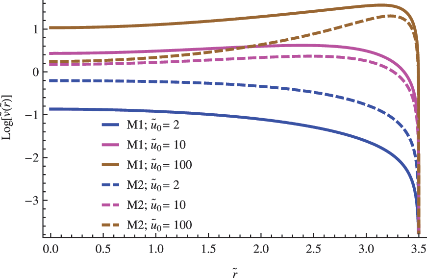
In addition to the observed impact on the critical radius, substrate concentration is another important element that affects the replicator's population. In general, we find that large substrate concentrations favor high levels of replicator's concentration (see Figs. 6 and 7). Once again, this tendency reinforces the fundamental role played by the nutrient availability on the successful establishment of a replicator population.
The influence of substrate concentration in the concentration profile for the replicator species. The other parameters were set to \documentclass{aastex}\usepackage{amsbsy}\usepackage{amsfonts}\usepackage{amssymb}\usepackage{bm}\usepackage{mathrsfs}\usepackage{pifont}\usepackage{stmaryrd}\usepackage{textcomp}\usepackage{portland, xspace}\usepackage{amsmath, amsxtra}\usepackage{upgreek}\pagestyle{empty}\DeclareMathSizes{10}{9}{7}{6}\begin{document}$$\left\{ { \widetilde R = 7; { \hbox { } } \left( { { \frac { { D_1 } } { { D_2 } } } } \right) = \left ( { \frac { d } { a } } \right) = 1 } \right\} $$ \end{document}.
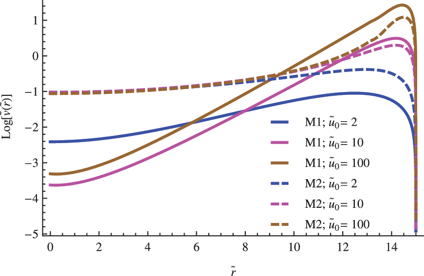
The influence of substrate concentration in the concentration profile for the replicator species. The other parameters were set to \documentclass{aastex}\usepackage{amsbsy}\usepackage{amsfonts}\usepackage{amssymb}\usepackage{bm}\usepackage{mathrsfs}\usepackage{pifont}\usepackage{stmaryrd}\usepackage{textcomp}\usepackage{portland, xspace}\usepackage{amsmath, amsxtra}\usepackage{upgreek}\pagestyle{empty}\DeclareMathSizes{10}{9}{7}{6}\begin{document}$$\left\{ { \widetilde R = 15; { \hbox { } } \left( { { \frac { { D_1 } } { { D_2 } } } } \right) = \left ( { \frac { d } { a } } \right) = 1} \right\} $$ \end{document}.
Figures 6 and 7 also show noticeable differences between the estimations derived from M1 and M2 models. Firstly, whereas the M2 model estimates the largest values of the replicator population when the substrate concentration is low, the situation changes when the availability of nutrients increases. In these cases, the largest estimations correspond to the M1 model. Secondly, we find that the estimations of the replicator population in the central region of the vesicle decrease faster for M1 than for the M2 model as the size of the vesicle increases (comparing Figs. 6 and 7). In general, both tendencies are driven by the differences in the contribution of the decays' terms contained in both models when the substrate concentration changes from low to high levels. Whereas the nonlinear decay included in the M2 model prevails when the substrate content in the medium is high, the linear decay included in the M1 model plays a major role when the substrate content is low.
4. Conclusions
The ability of a chemical replicator to inhabit a vesicle in extreme environments may be considered as an early stage of prebiotic systems. As we have seen throughout this work, such capabilities are determined in our minimal scenario by three main parameters: the availability of substrate, the diffusion constant of the replicator species, and the effectiveness of the replication process codified in the reproduction rate constant. These three parameters determine the existence of a critical radius of the vesicle under which the replicator population is no longer viable. In the case of a replicator model with linear decay, the ratio between deaths/births determines the required minimum value of substrate concentration above which the replicator population is always viable. Once again, even when our dynamic approach about the cell size differs from the classical ones (Newton-Harvey, 1928; Catling et al.,2005), the availability of substrates emerges as a central problem in a prebiotic scenario. Additionally, our results suggest that it is also improbable to inhabit extremely large vesicles partially due to a substantial dilution of the replicator species in the inner volume. According to Pross (2005a), the ratios between the diffusion constants substrate/replicator and the balance between birth/death processes can contribute positively (both are greater than the unity) or negatively (both are lower than the unity) to the robustness of the system.
Also, comparing our results with the Fisher-Kolgomorov estimations (F-K equation), we find that, even when both estimate the same values for the critical radius, this last model overestimates the concentrations of the replicator's populations in all studied cases. Such discrepancies are linked to an unrealistic assumption of an infinite diffusion rate of the substrate implicit in the F-K model.
In general, the idea of a replicator confined to a vesicle, even when it is not the only alternative (see for instance Walker et al. [2012]), is revealed as a promising research area. The processes of compartmentalization are usually considered as an effective mechanism of entropy reduction and self-organization in a biological system (Marín et al.,2009; Davies et al.,2013). However, according to our results, the effectiveness of these processes in extremely hostile environments could be limited at some minimal-length scale, with the system being unable to support the relatively complex chemical network involved in the replication. We must emphasize that the existence of a limiting size in our case is just the theoretical limit of self-suffocation of the replication mechanism inside the vesicle (Piedrafita et al.,2012), assuming idealistic conditions (without diffusive limitations across the membrane and the quick destruction of the replicator in the external medium). In any case, more detailed modeling is needed with the aim of building more realistic scenarios. The study of specific replicator systems, the inclusion of the transport processes across the cell boundary similar to that indicated by Piedrafita et al. (2017), and a relaxation of the environmental conditions used comprise some of these topics. Other important issues such as the origin of homochirality (Sandars, 2003) or the genetic code could be studied in a similar scenario. Much more work will need to be done to fully understand this amazing phenomenon that is life. Undoubtedly, it is a difficult task that will continue to inspire an entire generation of new researchers.
Footnotes
Acknowledgments
Y.L. acknowledges the support of this research by the Dirección de Investigación y Extensión Académica de la Universidad de Tarapacá under project No. 4729-16. C.G.-J. acknowledges the Pontificia Universidad Católica de Ecuador Sede Esmeraldas for financial support of the research.
Author Disclosure Statement
The authors declare no competing financial interests.
References
1.
AnetF.A.L. (2004) The place of metabolism in the origin of life. Curr Opin Chem Biol, 8:654–659.
2.
ArtilesW., CarvalhoP.G.S., and KraenkelR.A. (2008) Patch-size and isolation effects in the Fisher–Kolmogorov equation. J Math Biol, 57, doi:10.1007/s00285-008-0174-2.
3.
Bar-EvenA., NoorE., SavirY., LiebermeisterW., DavidiD., TawfikD.S., and MiloR. (2011) The moderately efficient enzyme: evolutionary and physicochemical trends shaping enzyme parameters. Biochemistry, 50:4402–4410.
4.
BartelD.P. and UnrauP.S. (1999) Constructing an RNA world. Trends Genet, 15, doi:10.1016/S0168-9525(99)01898-3.
5.
BennerS.A. (2010) Defining life. Astrobiology, 10:1021–1030.
6.
BoiteauL. and PascalR. (2011) Energy sources, self-organization, and the origin of life. Orig Life Evol Biosph, 41, doi:10.1007/s11084-010-9209-y.
7.
BrackA. (2007) From interstellar amino acids to prebiotic catalytic peptides: a review. Chem Biodivers, 4:665–679.
8.
CatlingD.C., GleinC.R., ZahnleK.J., and McKayC.P. (2005) Why O2 is required by complex life on habitable planets and the concept of planetary “oxygenation time.”. Astrobiology, 5:415–438.
9.
ChodasewiczK. (2014) Evolution, reproduction and definition of life. Theory Biosci, 133:39–45.
10.
CzáránT. and SzathmáryE. (2000) Coexistence of replicators in prebiotic evolution. In The Geometry of Ecological Interactions, edited by DieckmannU., LawR., and MetzJ.A.J., IIASA and Cambridge University Press, Cambridge, UK, pp 116–134.
11.
DaviesP.C.W., RieperE., and TuszynskiJ.A. (2013) Self-organization and entropy reduction in a living cell. Biosystems, 111:1–10.
12.
de la EscosuraA., BrionesC., and Ruiz-MirazoK. (2015) The systems perspective at the crossroads between chemistry and biology. J Theor Biol, 381:11–22.
13.
Del BiancoC. and MansyS.S. (2012) Nonreplicating protocells. Acc Chem Res, 45:2125–2130.
14.
DobovišekA., ŽupanovićP., BrumenM., Bonačić-LošićŽ., KuićD., and JuretićD. (2011) Enzyme kinetics and the maximum entropy production principle. Biophys Chem, 154:49–55.
15.
EhrenfreundP., SpaansM., and HolmN.G. (2011) The evolution of organic matter in space. Philos Trans A Math Phys Eng Sci, 369, doi:10.1098/rsta.2010.0231.
FerrisJ.P. (2005) Catalysis and prebiotic synthesis. Reviews in Mineralogy and Geochemistry, 59:187–210.
18.
FisherR.A. (1930) The Genetical Theory of Natural Selection, Oxford University Press, Oxford.
19.
GilbertW. (1986) Origin of life: the RNA world. Nature, 319, doi:10.1038/319618a0.
20.
GiomettoA., RinaldoA., CarraraF., and AltermattF. (2014) Emerging predictable features of replicated biological invasion fronts. Proc Natl Acad Sci USA, 111:297–301.
21.
HanczycM.M., MansyS.S., and SzostakJ.W. (2007) Mineral surface directed membrane assembly. Orig Life Evol Biosph, 37, doi:10.1007/s11084-006-9018-5.
22.
HernandezA.F. and GroverM.A. (2013) A necessary condition for coexistence of autocatalytic replicators in a prebiotic environment. Life, 3:403–420.
23.
KingG.A.M. (1982) Recycling, reproduction, and life's origins. Biosystems, 15:89–97.
24.
KingG.A.M. (1986) Was there a prebiotic soup?. J Theor Biol, 123:493–498.
25.
KleidonA. (2010) Life, hierarchy, and the thermodynamic machinery of planet Earth. Phys Life Rev, 7:424–460.
26.
KönnyűB. and CzáránT. (2013) Spatial aspects of prebiotic replicator coexistence and community stability in a surface-bound RNA world model. BMC Evol Biol, 13, doi:10.1186/1471-2148-13-204.
27.
LazcanoA. (2008) What is life? A brief historical overview. Chem Biodivers, 5, doi:10.1002/cbdv.200890001.
28.
LincolnT.A. and JoyceG.F. (2009) Self-sustained replication of an RNA enzyme. Science, 323:1229–1232.
29.
MaW. (2016) The essence of life. Biol Direct, 11, doi:10.1186/s13062-016-0150-5.
30.
MaW. and FengY. (2015) Protocells: at the interface of life and non-life. Life, 5:447–458.
31.
MarínD., MartínM., and SabaterB. (2009) Entropy decrease associated to solute compartmentalization in the cell. Biosystems, 98:31–36.
32.
MartínO. and HorvathJ.E. (2013) Biological evolution of replicator systems: towards a quantitative approach. Orig Life Evol Biosph, 43:151–160.
33.
MartínO., PeñateL., AlvaréA., CárdenasR., and HorvathJ.E. (2009) Some possible dynamical constraints for life's origin. Orig Life Evol Biosph, 39:533–544.
34.
MartinW., BarossJ., KelleyD., and RussellM.J. (2008) Hydrothermal vents and the origin of life. Nat Rev Microbiol, 6:805–814.
35.
Maynard-SmithJ. (1979) Hypercycles and the origin of life. Nature, 280, doi:10.1038/280445a0.
36.
MorowitzH.J., HeinzB., and DeamerD.W. (1988) The chemical logic of a minimum protocell. Orig Life Evol Biosph, 18:281–287.
37.
MulkidjanianA.Y., CherepanovD.A., and GalperinM.Y. (2003) Survival of the fittest before the beginning of life: selection of the first oligonucleotide-like polymers by UV light. BMC Evol Biol, 3, doi:10.1186/1471-2148-3-12.
38.
Newton-HarveyE. (1928) The oxygen consumption of luminous bacteria. J Gen Physiol, 11:1927–1928.
39.
PatelB.H., PercivalleC., RitsonD.J., DuffyColmD., and SutherlandJ.D. (2015) Common origins of RNA, protein and lipid precursors in a cyanosulfidic protometabolism. Nat Chem, 7:301–307.
40.
PiedrafitaG., MonteroF., MoránF., CárdenasM.L., and Cornish-BowdenA. (2010) A simple self-maintaining metabolic system: robustness, autocatalysis, bistability. PLoS Computat Biol, 6, doi:10.1371/journal.pcbi.1000872.
41.
PiedrafitaG., Ruiz-MirazoK., MonnardP.-A., Cornish-BowdenA., and MonteroF. (2012) Viability conditions for a compartmentalized protometabolic system: a semi-empirical approach. PLoS One, 7, doi:10.1371/journal.pone.0039480.
42.
PiedrafitaG., MonnardP.-A., MavelliF., and Ruiz-MirazoK. (2017) Permeability-driven selection in a semi-empirical protocell model: the roots of prebiotic systems evolution. Sci Rep, 7, doi:10.1038/s41598-017-02799-6.
43.
PigolottiS., BenziR., JensenM.H., and NelsonD.R. (2012) Population genetics in compressible flows. Phys Rev Lett, 108:128102.
44.
ProssA. (2005a) On the emergence of biological complexity: life as a kinetic state of matter. Orig Life Evol Biosph, 35:151–166.
45.
ProssA. (2005b) Stability in chemistry and biology: life as a kinetic state of matter. Pure Appl Chem, 77, doi:10.1351/pac200577111905.
46.
ProssA. (2011) Toward a general theory of evolution: extending Darwinian theory to inanimate matter. J Syst Chem, 2, doi:10.1186/1759-2208-2-1.
47.
ProssA. and KhodorkovskyV. (2004) Extending the concept of kinetic stability: toward a paradigm for life. J Phys Org Chem, 17:312–316.
48.
RobertsonM.P. and JoyceG.F. (2012) The origins of the RNA world. Cold Spring Harb Perspect Biol, 4, doi:10.1101/cshperspect.a003608.
WächtershäuserG. (2007) On the chemistry and evolution of the pioneer organism. Chem Biodivers, 4, doi:10.1002/cbdv.200790052.
60.
WaldeP., UmakoshiH., StanoP., and MavelliF. (2014) Emergent properties arising from the assembly of amphiphiles. Artificial vesicle membranes as reaction promoters and regulators. Chem Commun, 50:10177–10197.
61.
WalkerS.I., GroverM.A., and HudN.V. (2012) Universal sequence replication, reversible polymerization and early functional biopolymers: a model for the initiation of prebiotic sequence evolution. PLoS One, 7, doi:10.1371/journal.pone.003416.