
Abstract
The nearby exoplanet Proxima Centauri b will be a prime future target for characterization, despite questions about its retention of water. Climate models with static oceans suggest that Proxima b could harbor a small dayside surface ocean despite its weak instellation. We present the first climate simulations of Proxima b with a dynamic ocean. We find that an ocean-covered Proxima b could have a much broader area of surface liquid water but at much colder temperatures than previously suggested, due to ocean heat transport and/or depression of the freezing point by salinity. Elevated greenhouse gas concentrations do not necessarily produce more open ocean because of dynamical regime transitions between a state with an equatorial Rossby–Kelvin wave pattern and a state with a day–night circulation. For an evolutionary path leading to a highly saline ocean, Proxima b could be an inhabited, mostly open ocean planet with halophilic life. A freshwater ocean produces a smaller liquid region than does an Earth salinity ocean. An ocean planet in 3:2 spin–orbit resonance has a permanent tropical waterbelt for moderate eccentricity. A larger versus smaller area of surface liquid water for similar equilibrium temperature may be distinguishable by using the amplitude of the thermal phase curve. Simulations of Proxima Centauri b may be a model for the habitability of weakly irradiated planets orbiting slightly cooler or warmer stars, for example, in the TRAPPIST-1, LHS 1140, GJ 273, and GJ 3293 systems.
1. Introduction
T
In contrast, Proxima b closely orbits a red dwarf star. This would probably have driven it into a runaway greenhouse state during the star's luminous premain sequence phase, and even today would subject it to X-ray and extreme ultraviolet fluxes and stellar winds that might lead to catastrophic atmospheric and surface water loss (Ribas et al., 2016; Airapetian et al., 2017; Barnes et al., 2017; Dong et al., 2017; MacGregor et al., 2018). Nonetheless, Proxima b has a poorly constrained and potentially complex evolutionary history. Depending on its initial water inventory, the presence of an initial shielding hydrogen envelope, velocities of previous impacts, and whether it migrated to its current position from a greater distance, scenarios exist by which the planet could be habitable (Ribas et al., 2016; Barnes et al., 2017; Zahnle and Catling, 2017).
It is, thus, worthwhile to use existing constraints to assess whether hypothetical atmospheres for Proxima b are conducive to life. Meadows et al. (2018) simulated a broad range of 1-D photochemically consistent climates for Proxima b. Turbet et al. (2016) used a 3-D general circulation model (GCM) with a dry land surface, ice surface, or static thermodynamic ocean. They found “eyeball Earth” climates (Pierrehumbert, 2011) with substellar warm liquid water for an atmosphere similar to modern Earth's if Proxima b synchronously rotates, but required elevated CO2 to maintain an equatorial waterbelt if the planet is in 3:2 spin–orbit resonance. Boutle et al. (2017) used a different GCM with an atmosphere bounded by a 2.4 m liquid surface and irradiated by a slightly lower stellar flux than that used by Turbet et al. (2016). [The 881.7 W/m2 used by Boutle et al. (2017) matches the best estimate of Anglada-Escudé et al. (2016), but the 956 W/m2 used by Turbet et al. (2016) is within the uncertainties.] Their model produces similar climates to those of Turbet et al. (2016) but with cooler dayside and much colder nightside temperatures. Boutle et al. (2017) found that if spin–orbit resonance occurs with significant eccentricity, two eyeball regions of surface liquid water exist on opposite sides of the planet, the sides that face the star at successive periastrons (Dobrovolskis, 2007; Brown et al., 2014).
The assumption of a static ocean is computationally convenient (and is thus the standard for GCM exoplanet studies), but does not capture much of the physics by which oceans modulate climate. Hu and Yang (2014) coupled a dynamic ocean to an exoplanet GCM to show that ocean heat transport broadens the region of surface liquid water. Yang et al. (2014) used dynamic ocean, sea ice, and land ice models to explore water trapping on the nightside of a synchronously rotating planet. Cullum et al. (2016) used an ocean GCM to emphasize the role that varying salinity might play in determining exoplanet climates.
In this article, we present the first simulations of potential Proxima Centauri b climates using an atmospheric GCM coupled to a dynamic ocean GCM. We consider shallow all-ocean “aquaplanets” and planets with a modern Earth-like land–ocean distribution. Section 2 describes our model and experiments, and the resulting climates are analyzed in Section 3. The implications for Proxima Centauri b, and for exoplanet habitability in general, are discussed in Section 4.
2. Methods
2.1. Model description
We use the ROCKE-3D (Resolving Orbital and Climate Keys of Earth and Extraterrestrial Environments with Dynamics) GCM (Way et al., 2017), a planetary adaptation of the NASA Goddard Institute for Space Studies (GISS) Model E2 Earth GCM. ROCKE-3D has been used to simulate a potential habitable ancient Venus (Way et al., 2016), the climate response to long-term evolution of planetary eccentricity (Way and Georgakarakos, 2017), factors controlling the onset of moist greenhouse stratospheric conditions on aquaplanets (Fujii et al., 2017), and possible snowball periods in Earth's past (Sohl and Chandler, 2007).
For the experiments described here, ROCKE-3D was run with an atmosphere at 4° × 5° latitude–longitude resolution and 40 vertical layers with a top at 0.1 hPa. This resolution should be adequate, given the rotation period of Proxima Centauri b (11.2 days for synchronous rotation, 7.5 days for 3:2 spin–orbit resonance), near or beyond the threshold at which baroclinic eddies reach planetary size and the atmospheric dynamics transitions from a rapidly rotating to a slowly rotating regime (Del Genio and Suozzo, 1987; Edson et al., 2011).
We use the SOCRATES (
Wavelength Ranges (μm) for the Archean Simulations Using 29 Shortwave and 12 Longwave Bands
Wavelength Ranges (μm) for the Control-Thick Simulation Using 43 Shortwave and 15 Longwave Bands
Wavelength Ranges (μm) for the Pure CO2 Simulation Using 42 Shortwave and 17 Longwave Bands
Description of General Circulation Model Simulations
Simulations with an * use 29/12 shortwave/longwave radiation bands; that with a # uses 43/15 shortwave/longwave bands; and that with a + uses 42 shortwave and 17 longwave bands; all others use 6/9 shortwave/longwave bands. Simulations with a @ use the MT_CKD 3.0 continuum.
e, eccentricity; S o, stellar constant; S, salinity.
ROCKE-3D also employs a mass flux cumulus parameterization with two updraft plumes of differing entrainment rates, convective downdrafts, and interactive lifting and detrainment of convective condensate into anvil clouds; a stratiform cloud scheme with prognostic condensate, diagnostic cloud fraction, and cloud optical properties based on simulated liquid and ice water contents and a temperature-dependent ice crystal effective size (Edwards et al., 2007); and a dry turbulent boundary layer scheme with nonlocal turbulence effects, all described further by Way et al. (2017).
Tian and Ida (2015) found that ocean planets and desert planets are more likely to exist than planets with partially exposed land in systems orbiting low-mass stars. Nonetheless, given Proxima b's unknown history, we consider several possible scenarios. For most simulations, the atmosphere is bounded by a dynamic aquaplanet ocean having the same horizontal resolution as the atmosphere and nine layers extending to 900 m depth, much shallower than the ∼3700 m mean depth of Earth's oceans. This is primarily done for computational convenience—even with a fairly shallow ocean, our experiments can require ∼1000–5000 orbits (∼30–150 Earth years) to reach equilibrium. Nonetheless, even at 900 m depth, the ocean heat capacity (which is proportional to depth) implies a thermal response time to radiative forcing that is much longer than the rotation period of Proxima b. This is important for asynchronously rotating scenarios.
Isopycnal transport by unresolved ocean eddies is parameterized by a unified Redi/Gent-McWilliams (GM) scheme (Redi, 1982; Gent and McWilliams, 1990; Gent et al., 1995). A background diapycnal vertical diffusion with diffusivity 0.3 cm2/s is based on the KPP (K-Profile Parameterization) scheme (Large et al., 1994). For Earth, unresolved eddies matter for ocean meridional overturning and the Antarctic Circumpolar Current (Hallberg and Gnanadesikan, 2006; Bryan et al., 2014; Marshall et al., 2017). The coarse ocean resolution we use here was employed in the terrestrial version of the GISS GCM as recently as in the work of Hansen et al. (2007), who found that it satisfactorily represented the ocean overturning circulation but was inadequate for tropical intraseasonal variability.
It is not known how applicable such approaches are for oceans on slowly rotating planets, where the spatial scale of the relevant eddies should differ from those on Earth. If the ocean eddy scale is set by the baroclinic Rossby radius of deformation (L or), which is inversely proportional to rotation (in the extratropics) or its square root (in the tropics), the relevant eddies should be ∼3–10 times larger on Proxima Centauri b due to its slow (11.2 days) rotation period. On Earth, L or ∼150–250 km in the equatorial region and ∼10–30 km at high latitudes (Chelton et al., 1998). Thus, in the equatorial region at least, eddies may be resolved by the model, even more so on the dayside because of the strong stabilization of the upper ocean by the fixed stellar heating. The GM transport in our experiments is two to three orders of magnitude weaker than the resolved transport, suggesting that at our slow rotation eddies are not a controlling factor. A sensitivity test that replaces the nominal 1200 m2/s GM diffusivity with a much lower value (100 m2/s) changes maximum and minimum surface temperatures by no more than half a degree. Unlike Earth, however, where eddy-resolving models provide a benchmark for assessing coarser resolution GCMs, only a few studies of ocean circulation exist yet for planets with different rotation periods (Vallis and Farneti, 2009; Cullum et al., 2014; Hu and Yang, 2014), and none to our knowledge focus on how mesoscale eddies respond to a change of rotation.
Ocean albedo is spectrally dependent and varies with solar zenith angle and wind speed. Typical substellar values for the diffuse/direct components are 0.072/0.039 for wavelengths λ < 0.770 μm and 0.056/0.032 at longer λ, respectively. Absorption beneath the ocean surface is parameterized with a red/near-IR component with e-folding penetration depth of 1.5 m and a shorter wavelength component with e-folding depth of 20 m, weighted by the solar spectrum for an average turbidity of seawater.
The ocean model includes a dynamic sea ice parameterization (see Way et al., 2017) with albedos in one visible and five near-IR spectral intervals that vary with ice thickness, the presence, depth, age, and type (dry or wet) of snow, the presence of melt ponds, and zenith angle. Seawater freezes at a temperature that depends on salinity. Fractional gridbox sea ice cover is permitted.
For simulations with continents, the land surface has an albedo of 0.2, typical of a terrestrial desert. The soil texture is assumed to be a mixture with sand/silt/clay fractions of 0.5/0.0/0.5 (as in Way et al., 2016), giving a porosity of 0.4855 pore volume over soil volume. The GISS land surface model has a depth of 3.5 m, so with this soil texture, maximum soil water content is 1699 kg/m2. Given the lack of seasons in our simulations, soil moisture memory that could arise from different soil textures does not have an influence on our climate. Land areas can accumulate snow up to a specified limit of 2 m water equivalent, with amounts above this transported to the ocean; land ice dynamics are not included. Lakes form when input from soil runoff and river inflow exceeds output from river outflow. Soil runoff is from the surface when precipitation exceeds infiltration and from subsurface runoff from soil with a nonzero slope. A formed lake also has inputs from precipitation and losses from evaporation. Lake size is dynamic according to the balance of these inputs and outputs. The ocean in these partially exposed land experiments is assumed to have flat bathymetry, with no islands.
Planetary properties for Proxima b are identical to those used by Turbet et al. (2016): gravity = 10.98 m/s2 and radius = 7127.335 km, based on assumptions that the planet mass M p = 1.4 M⊕ and the planet density ρ = ρ⊕ = 5.513 g/cm3. We use the Proxima Centauri stellar spectrum created by the Virtual Planetary Laboratory and described by Meadows et al. (2018).
2.2. Experiments
Table 4 describes our simulations. Our baseline experiment, Control, assumes a 0.984 bar atmosphere (Earth's mean surface pressure), primarily N2 but with 376 ppmv CO2, an aquaplanet dynamic ocean, synchronous rotation (11.2 days period), and the instellation value of Boutle et al. (2017). Salinity is initialized at a typical Earth value of 35.4 psu (practical salinity units, equivalent to grams of salt per kilogram of water, or 35.4 g/L, or 3.54%). Other experiments use Control as the baseline unless otherwise specified. To isolate the effect of the dynamic ocean, we perform a simulation with a 100 m thermodynamic ocean with no ocean heat transport (Thermo). Control-High uses the higher instellation value assumed by Turbet et al. (2016). Three Archean simulations assume a 0.984 bar N2-dominated atmosphere with elevated greenhouse gas concentrations based on previous studies of Archean Earth. Archean Med assumes the CO2 and CH4 abundances of Case A of Charnay et al. (2013). Archean Low assumes CO2 and CH4 levels half way between those of Control and Archean Med. Archean High has CO2 and CH4 concentrations identical to those indicated by Charnay et al. (2013) Case B. In addition, we perform one experiment with a pure 0.984 CO2 atmosphere (Pure CO2 ). Sensitivity to atmospheric thickness is tested in simulations Control-Thin (0.1 bars N2) and Control-Thick (10 bars N2), while the effect of ocean depth is explored in Control-Shallow (158 m depth) and Control-Deep (2052 m depth).
Two experiments test the effect of ocean salinity (S), based on the study of Cullum et al. (2016): S = 0 psu (Zero Salinity) and S = 230 psu (High Salinity), a value almost as high as that of the Dead Sea and in the range for extreme halophiles (Ollivier et al., 1994; Oren, 2002). The 230 psu value is a bit less than that used by Cullum et al. (2016) since our simulations are for a colder planet; it is slightly smaller than the 233 psu eutectic point value for an NaCl–H2O mixture, ensuring that our ocean remains below salt saturation. We explore climates for a 3:2 spin–orbit resonance planet with orbital eccentricity e = 0 (3:2e0) and e = 0.30 (3:2e30). Two experiments assume Earth-like continents, one with the substellar point over the dateline (180°) and thus dayside heating of a mostly enclosed ocean basin (Day-Ocean), and another with the substellar point at 30°E longitude and thus dayside heating of Africa and parts of Eurasia (Day-Land).
3. Results
Table 5 lists relevant climate variables for each simulation. All except one produce a regionally habitable surface climate as judged by the presence of areas with time mean temperature above the freezing point of seawater. Despite this, the planetary mean surface temperature for each simulation except one is below freezing, in some cases by tens of degrees. Thus, judged by traditional 1-D surface habitable zone criteria, most of the planets would not be considered habitable. Maximum surface temperatures in the substellar region differ by 34°C among the simulations, due to factors other than instellation or atmospheric composition differences. The global sea ice (or sea ice+snow for simulations with land) cover ranges from 0% to 80%. Minimum temperatures vary more (by 96°C), reflecting the control of nightside temperatures by heat and moisture transports (Yang and Abbot, 2014), as well as noncondensing greenhouse gases, which vary considerably (by design) among the experiments.
Climate Variables for Each Experiment: Maximum, Minimum, and Mean Surface Temperature (T surf), Fraction of Surface Not Covered by Sea Ice or Snow (f hab), Equilibrium Temperature (T eq), Planetary Albedo (A p), Maximum Water Vapor Volume Mixing Ratio at p = 0.1 p surf (H2O)
Ocean freezing points are 0°C for S = 0 psu, −1.9°C for S = 35.4 psu, and −19°C for S = 230 psu.
3.1. Synchronously rotating aquaplanets with an Earth-like ocean and atmosphere
Figures 1a and 2a show the surface temperature and sea ice cover, respectively, for Control. These differ greatly from the “eyeball” pattern of substellar liquid water found by Turbet et al. (2016) and Boutle et al. (2017). Control instead produces a “lobster” pattern of open ocean water that is characteristic of simulations of synchronously rotating planets with a dynamic ocean. As explained by Hu and Yang (2014), this is a realization of the Matsuno (1966) and Gill (1980) pattern of atmospheric response to a stationary heat source. Such a heat source generates a Rossby wave-induced cyclonic circulation on either side of the equator west of the heat source and an equator-straddling Kelvin wave east of the heat source (Fig. 3a). The Rossby wave circulation moves warm substellar water away from the equator (Fig. 3b), keeping temperatures above freezing at higher latitudes. East of the substellar point, the Kelvin wave, a circulation in the longitude-altitude plane, produces no corresponding meridional heat advection. This produces the asymmetric pattern of surface temperature and open ocean about the substellar point. The surface wind converges near the instellation maximum (Fig. 3a), away from the equator in the Rossby wave region and near the equator in the Kelvin wave region, leading to rising motion and the onset of moist convection and thick clouds (Section 4b) that shield the surface from incident starlight (Yang et al., 2013) but also provide LW warming.

Surface temperature distributions (°C) for

As in Figure 1 but for sea ice cover (%).
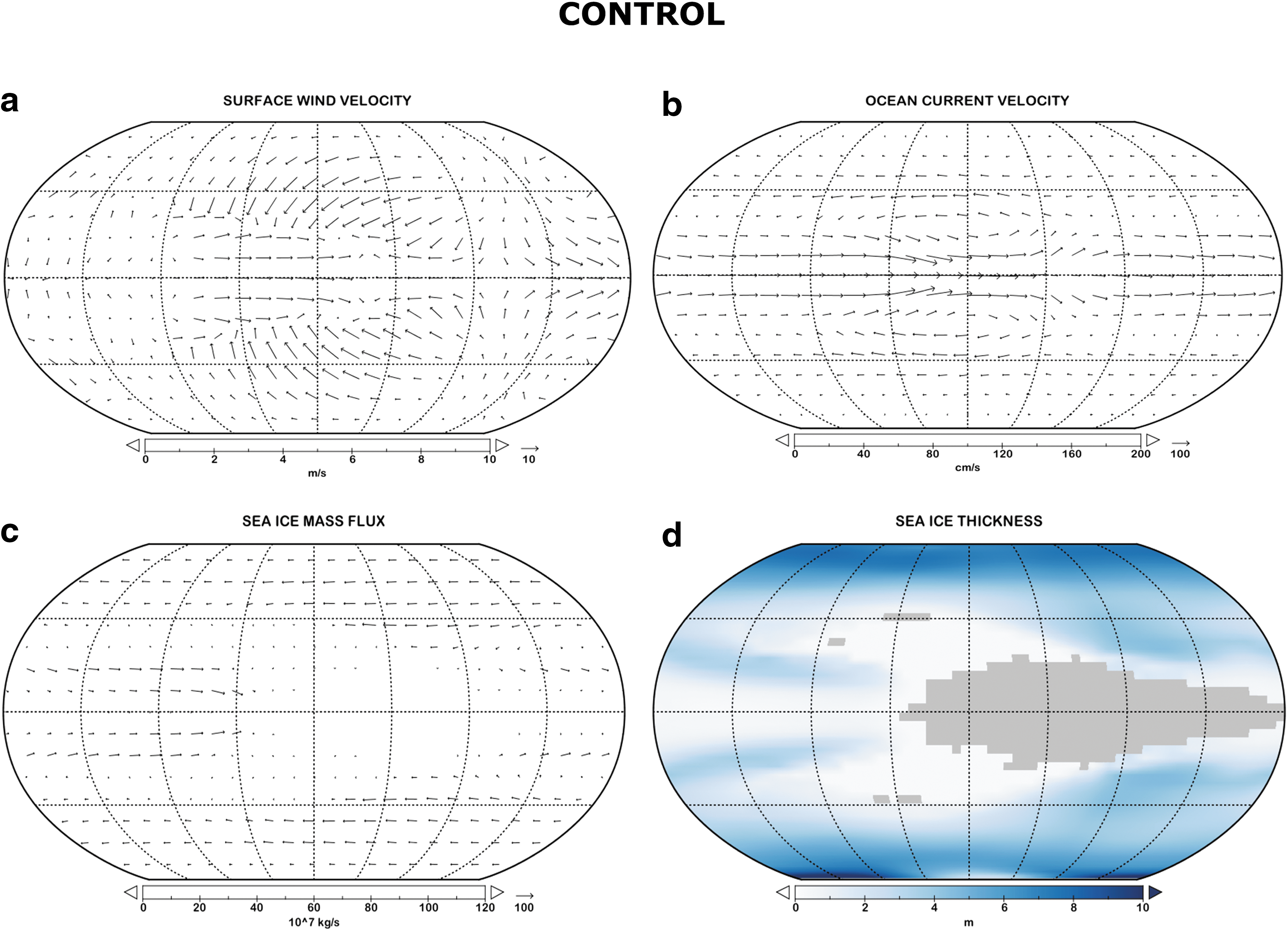
Control experiment distributions of
The near-surface ocean in Control develops a mostly westerly equatorial current (Fig. 3b) that advects warm water downstream (and away from the equator near the substellar point), and keeps the equatorial ocean at least partly ice free all the way to the antistellar point and beyond. Our result is similar to that of Hu and Yang (2014), but for their bigger, more slowly rotating planet, the westerly current does not maintain above-freezing equatorial temperatures over all longitudes. Upstream of the instellation peak, strong advection of sea ice into the substellar region (Fig. 3c) and subsequent melting keep equatorial temperatures slightly cooler than on either side of the equator. The ocean is completely ice free only in a tropical region near the evening terminator (Fig. 3d). Because of the night-to-day sea ice mass flux, sea ice thickness on the nightside remains below 10 m (Fig. 3d). The net result of the atmospheric, oceanic, and sea ice transports is a peak dayside surface temperature (3°C) that is much cooler than the ∼27°C found by Turbet et al. (2016) for the same atmospheric composition but a slightly higher instellation and thermodynamic ocean. The liquid water-sustaining fraction of the surface f hab, defined here as the fraction without sea ice (or sea ice+snow, for the experiments with land described later), is 0.42.
Figures 1b and 2b show surface temperature and sea ice, respectively, for the static ocean case Thermo. The maximum temperature (19°C) is much warmer than that of Control despite identical atmospheric composition, and its minimum is even more dramatically colder, due to the absence of ocean heat transport. Our dayside maximum is comparable with that of Boutle et al. (2017) but ∼10°C colder than that of Turbet et al. (2016) who used an instellation 74.3 W/m2 larger. Our dynamic ocean simulation with the higher (Turbet et al. 2016) instellation value (Control-High) has a dayside maximum only 3°C warmer than Control with a similar pattern of surface temperature and sea ice but a larger area of open ocean due to the stronger instellation (Figs. 1c and 2c), which illustrates the damping effect of a dynamic ocean on the climate response to external forcing. Larger differences occur on the nightside: Our minimum temperature decreases by 30°C without ocean heat transport and increases by 8°C when instellation is increased, but in neither case do we approach the very cold nightside temperatures (−123°C) found by Boutle et al. (2017).
Our simulations start from a warm (285 K) isothermal atmosphere initial condition. Ferreira et al. (2011) and Popp et al. (2016) found that atmosphere-ocean GCMs can exhibit hysteresis behavior depending on whether the model is given a “warm start” or “cold start.” To test this, we used an instellation half that for Proxima Centauri b (440.9 W/m2) to create a snowball planet, and then reran Control with the cold start initial condition. Surface temperature, liquid water area fraction, and planetary albedo in equilibrium for this simulation are virtually identical to those in Control, as is the spatial pattern of open ocean. This is in agreement with the work of Checlair et al. (2017) who argued that bistability does not occur for synchronously rotating planets due to their unique spatial pattern of instellation.
3.2. Effect of elevated greenhouse gas concentrations
Our Archean experiments are not surprisingly warmer than Control (Table 5), but the progression in surface temperature as greenhouse gases increase from Low to Med to High is not monotonic except for the nightside minimum. The added dayside surface warming from CO2 and CH4 is weak (only 2–3°C warmer peak temperatures). In other respects, the Archean simulations differ from others in surprising ways. For example, despite being globally warmer, Archean Med is actually colder at the equator away from the substellar region (Fig. 1d). Its sea ice cover is slightly greater than Control (Fig. 2d) and much greater than Archean Low (Table 5), and it thus has a smaller liquid water fraction (f hab = 0.38) despite higher greenhouse gas concentrations. Archean Med has somewhat more ice-free area than Control at high latitudes, but lacks the equatorial band of open ocean water on the nightside.
This seemingly counterintuitive behavior is due to competition between the radiative effect of increasing greenhouse gases and changes in the atmospheric dynamical response to instellation from a cool star as the composition changes. Table 6 summarizes some of the relevant aspects of this competition. Instellation is identical in Control and the Archean simulations, but atmospheric absorption of the mostly near-IR flux of Proxima Centauri by the addition of CH4 in the Archean simulations increases. Thus, progressively less SW is absorbed at the surface at the dayside peak and more at high altitude. Combined with the added LW greenhouse effect, the result is an increasingly statically stable substellar temperature profile from Control to Archean Low to Archean Med to Archean High. Figure 4 shows this for Control versus Archean Med.
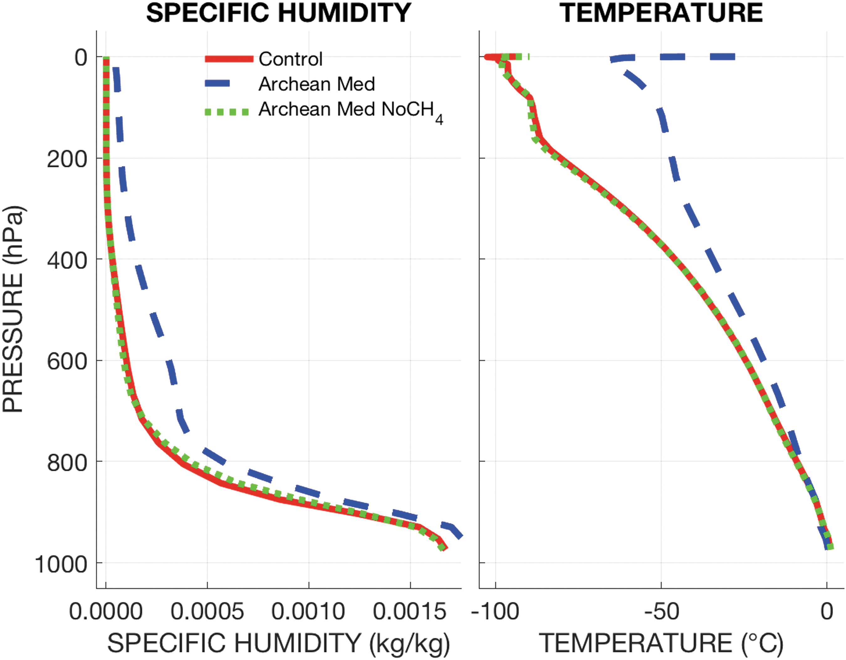
Substellar point vertical profiles of (left) specific humidity (kg H2O kg air−1) and (right) temperature (°C) for the Control, Archean Med, and Archean Med NoCH4 simulations.
Parameters Related to the Dynamical Regime Shift from the Control Simulation to the Four Archean Simulations
Several previous studies have explored the effect of rotation on the atmospheric dynamics of synchronously rotating rocky planets. Noda et al. (2017) identified a transition at ∼20 days rotation period between a dynamical regime dominated by a day–night circulation with weak zonal winds at longer periods and a regime characterized by a Matsuno–Gill Rossby–Kelvin wave response to the substellar heating and equatorial super-rotating winds at somewhat shorter periods. Edson et al. (2011) found a similar transition at ∼4–5 days rotation. Neither study is a direct analogue of ours; for example, neither assumes a dynamic ocean or a cool star spectrum. Nonetheless, the regime transition in both studies may be relevant to the differences between our Control and Archean climates.
Control is clearly in the Rossby–Kelvin regime. The upper troposphere has a strong wavenumber 1 standing oscillation (Fig. 5a) with the anticyclone centered near/downwind of the substellar region and cyclones at high latitudes on the nightside (see Fig. 6b, c of Noda et al., 2017). The NW–SE tilt of the flow in the northern hemisphere and SW–NE tilt in the southern hemisphere downstream of the substellar point create a strong equatorward flux of zonal momentum by eddies (Fig. 5c), similar to that seen for slowly rotating hot Jupiters (Showman et al., 2015, their Fig. 7a). This produces strong (∼60 m/s) nightside equatorial super-rotation (Fig. 5e and Table 6), as predicted by Showman and Polvani (2010, 2011). Between the evening terminator and antistellar point fairly strong subsidence (not shown), the downward branch of the Kelvin wave, advects potentially warm air from the dayside downward. This extends the super-rotation to the surface (Fig. 5e), helping to maintain above-freezing equatorial ocean temperatures there.

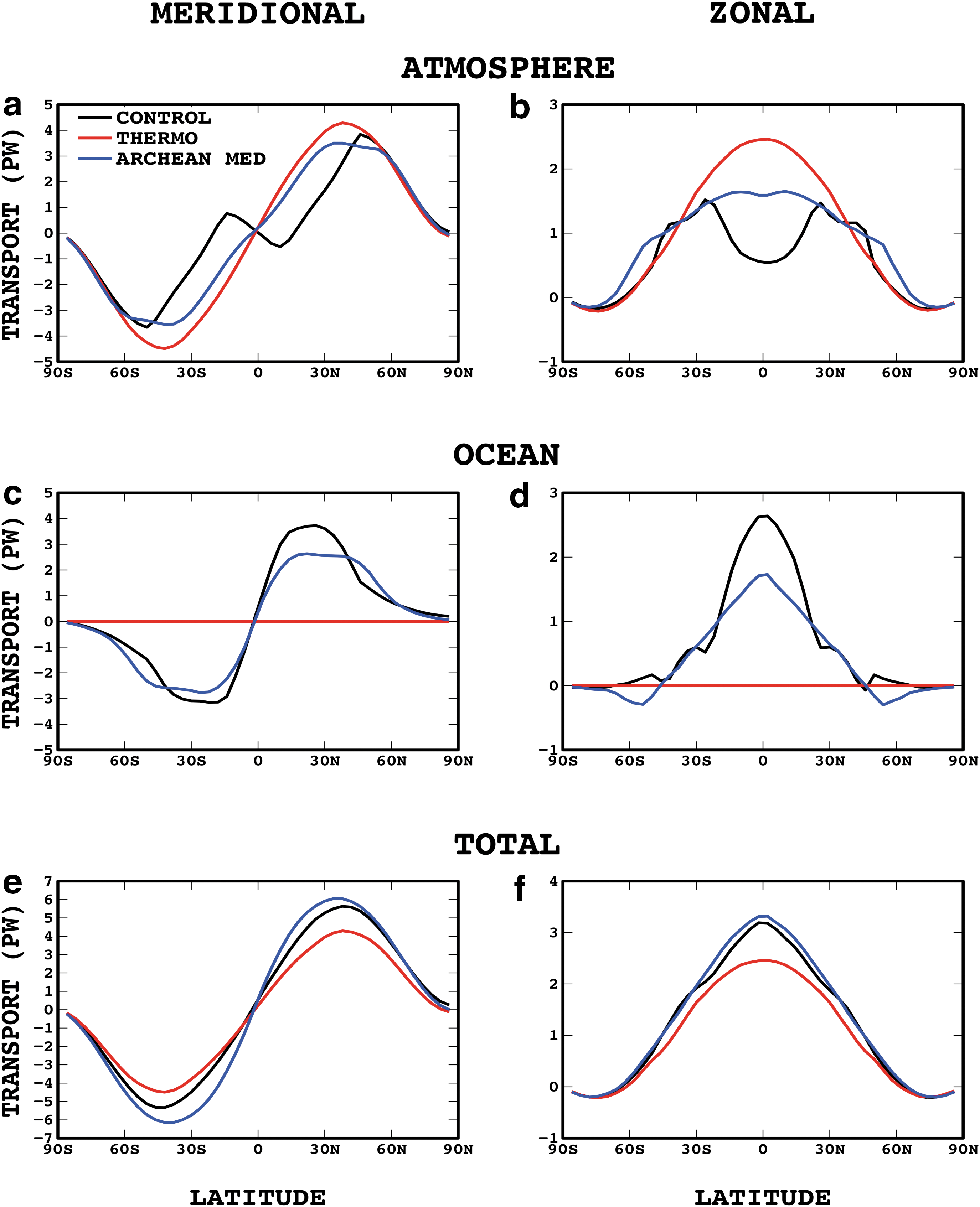
Vertically integrated (left) meridional and (right) zonal heat transports in petawatts PW (where 1 PW = 1015 W) by the
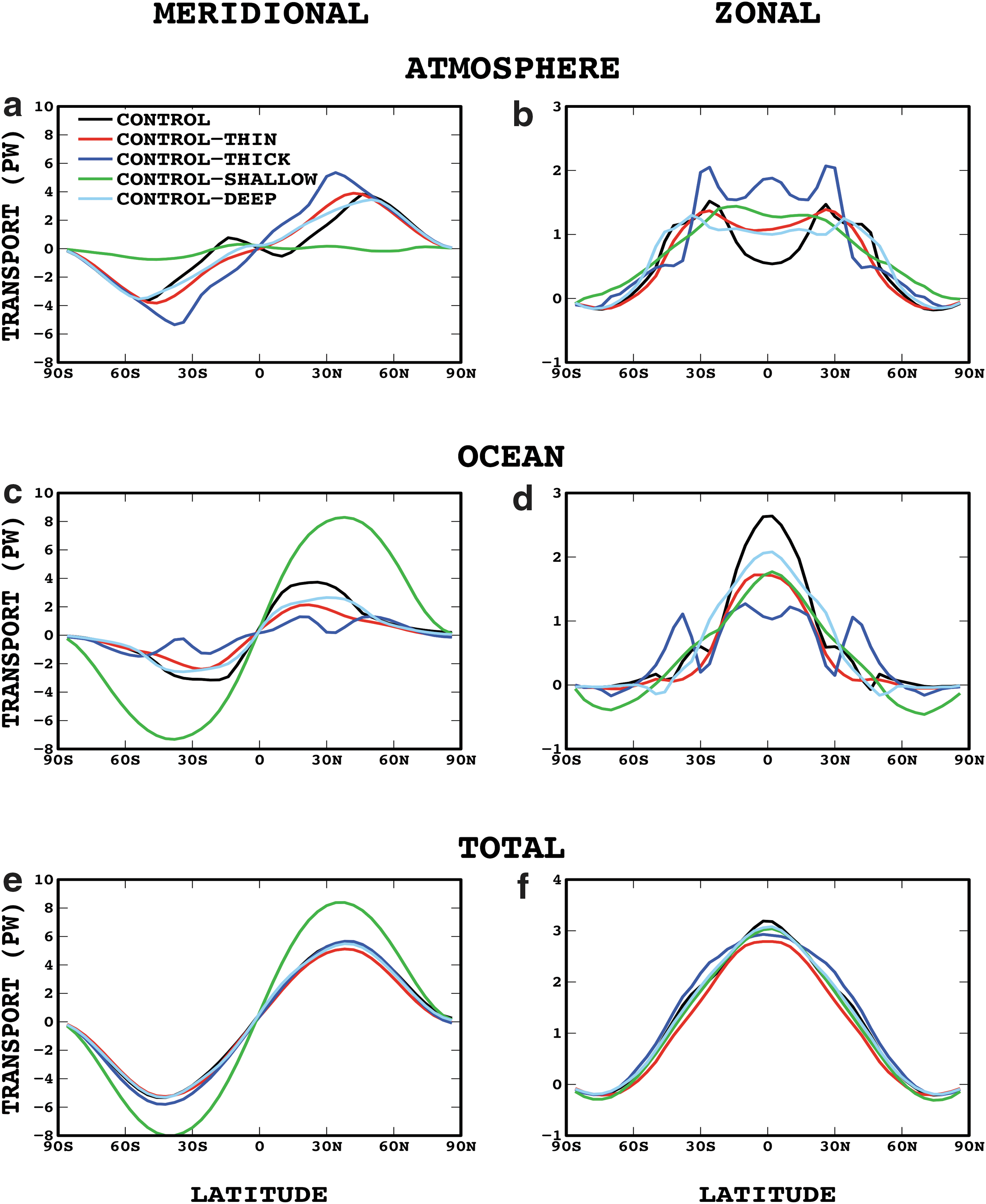
As in Figure 6 but for experiments Control, Control-Thin, Control-Thick, Control-Shallow, and Control-Deep.
The Archean simulations also appear to be in the Rossby–Kelvin regime, but barely so; Figure 5 shows analogous fields for Archean Med. Relative to Control, Archean Med exhibits only a weak stationary wave (Fig. 5b), much weaker equatorward eddy momentum transports (Fig. 5d), and consequently weaker (∼30 m/s) super-rotation (Fig. 5f and Table 6). Near the surface, Archean Med exhibits a pure day–night circulation more like that of the almost nonrotating regime of Noda et al. (2017) (see their Fig. 5a) and much weaker nightside subsidence. Thus, there is less adiabatic warming of descending air and no transport of dayside near-surface air to the nightside. As a result, the equatorial ocean surface remains frozen on the nightside and into the morning on the dayside, increasing sea ice cover. Archean Low and Archean High show similarly weak eddy momentum fluxes and equatorial super-rotation (Table 6).
Edson et al. (2011) argued that the regime transition from Rossby–Kelvin to day–night occurs as the atmospheric Rossby radius of deformation approaches the radius of the planet. For equatorial waves, the deformation radius is L d = (NH/β)1/2, where N = [(g/Θ)∂Θ/∂z]1/2 is the Brunt–Väisälä frequency, g is gravity, Θ is potential temperature, z is altitude, H is the scale height, β = 2Ω/a is the meridional gradient of the Coriolis parameter at the equator, Ω is the rotational angular frequency, and a is the planet radius. In the experiments of Edson et al. (2011) and Noda et al. (2017), the regime transition is accomplished by increasing the rotation period (thus increasing L d by decreasing β). In our synchronous rotation simulations, the rotation period is fixed. L d changes instead because the temperature and lapse rate change as greenhouse gases increase (Fig. 4), as seen in other studies of M star planets (Shields et al., 2013; Rugheimer et al., 2015). For our Proxima Centauri b simulations, a = 7127 km. We estimate that L d <a for Control and L d >a for Archean Low, Med, and High, although by modest amounts (Table 6). Furthermore, for Archean Med and Archean High, although the simulations are in equilibrium when averaged over sufficiently long timescales, significant variability remains on timescales of ∼3–8 Earth years, with global surface temperature fluctuating by up to ∼5°C and sea ice fraction by up to ∼15% (absolute). In addition, we find that small changes in model physics such as removing the spectral dependence of sea ice albedo can cause the Archean Med climate and circulation to change significantly. This supports our impression that the Archean climates are close to the regime transition and may exhibit bistable behavior, as Edson et al. (2011) found near the transition point.
Archean Med has higher maximum and minimum temperatures than Control but more sea ice (Table 5). Thus, it must be the dynamical response to the static stability change caused by CH4, rather than the direct radiative effect of CH4, that explains these results. We performed an experiment that removes the CH4 from the Archean Med atmosphere (Archean Med NoCH4 ). The substellar temperature profile in this simulation is almost identical to that in Control (Fig. 4), as are the circulation diagnostics analogous to those in Figure 5 and Table 6.
In the lower stratosphere, the Archean climates are tens of degrees warmer than Control due to the presence of CH4. This allows stratospheric H2O to build up to levels two orders of magnitude greater than in our other simulations, which does not occur when CH4 is removed (Fig. 4 and Table 5). This is still ∼10 times smaller than the traditional moist greenhouse water loss limit (Kasting et al., 1993), but it suggests that regardless of an early superluminous phase or XUV (X−rays + extreme ultraviolet) irradiation of the planet from its star, an aquaplanet Proxima Centauri b with sufficiently higher CH4 abundance may experience significant water loss by the traditional diffusion-limited escape mechanism.
We performed an additional simulation with a pure 1 bar CO2 atmosphere (Pure CO2 ). This simulation includes CO2–CO2 collisionally induced absorption following the works of Gruszka and Borysow (1998), Baranov et al. (2004), and Wordsworth et al. (2010), and CO2 sub-Lorentzian line shapes from the works of Perrin and Hartmann (1989) and Wordsworth et al. (2010). Turbet et al. (2016) found that such a planet has surface temperatures above freezing planet-wide even with a static ocean. Our results with a dynamic ocean are fairly similar (Table 5): A minimum temperature of 6°C and the highest mean surface temperature of any of our experiments (11°C). However, with ocean heat transport and the lower instellation value we use, the maximum temperature (18°C) is only comparable with or cooler than several other simulations and much colder than those found by Turbet et al. (2016).
Figure 6 shows profiles of meridional and zonal heat transport in the atmosphere, ocean, and their sum for Control, Thermo, and Archean Med. Stone (1978) argued that total meridional heat transport is mostly invariant to changes in the atmosphere and ocean, depending on external parameters such as the solar constant, planet radius, and obliquity, and peaks at ∼35° latitude. The one internal parameter that affects the transport in his theory is planetary albedo, as also found by Enderton and Marshall (2009) for cold planets with significant sea ice.
Figure 6 (and companion Figures 7 and 11 for other simulations) shows that the partitioning between atmosphere and ocean heat transport, and between meridional and zonal transport, varies considerably among the experiments, but the total transport is remarkably invariant with only a couple of exceptions and peaks near the latitude predicted by Stone (1978). The invariance holds separately for the meridional and zonal components of transport. One exception is Thermo, which has a higher albedo than all but one experiment (Table 5) and weaker total transport meridionally and zonally; that is, the lack of ocean transport is not fully compensated by the atmosphere. In contrast, Control and Archean Med, despite occupying different dynamical regimes, have almost identical total transports meridionally and zonally. The different fractional area of open water in these experiments is due to stronger equatorial ocean heat transport in Control.

As in Figure 6 but for experiments Control, Zero Salinity, High Salinity, Day-Ocean, and 3:2e30.
3.3. Effect of atmospheric thickness
Figures 1e and 2e show surface temperature and sea ice cover for simulation Control-Thin. This planet has an N2 atmosphere with 376 ppmv CO2, as in Control, but with a total surface pressure of only 0.1 bar. Likewise, Control-Thick (Figs. 1f and 2f) differs from Control only by having a total pressure of 10 bars. We keep the CO2 mixing ratio constant in these experiments rather than the partial pressures, so these planets, relative to Control, have a weaker/stronger greenhouse effect due to the lesser/greater amount and pressure broadening of CO2, although this is slightly offset by the lesser/greater atmospheric Rayleigh scattering.
Control-Thin is, thus, a cooler, brighter planet with little open ocean on the nightside, little upstream of the substellar point (compare Figs. 3e and 3a) and smaller liquid water area overall (Table 5), though its dayside temperature and sea ice retain the asymmetry caused by the Rossby–Kelvin wave pattern. Control-Thick is a warmer, darker planet with a planet-wide tropical band of liquid water. Atmospheric thickness has fairly little effect on total meridional or zonal transport (Fig. 7), only on its partitioning: Thick transports more heat in the atmosphere, but this is mostly compensated by the stronger oceanic transport in Thin. Control is something of an outlier: Because it maintains a thin equatorial liquid water band, it has efficient zonal ocean heat transport and weaker atmospheric zonal transport.
Control-Thin has much more stratospheric H2O than any other simulation (Table 5). This has been explained by Turbet et al. (2016), who found a qualitatively similar result with a different GCM, although our mixing ratios are somewhat lower than theirs presumably because of our cooler dayside temperatures. As pointed out by Turbet et al., this implies that water loss should be more rapid on planets with thin atmospheres.
3.4. Effect of ocean depth
Making the ocean shallower (158 m, Control-Shallow) and deeper (2052 m, Control-Deep) has only a small effect on globally averaged climate properties, producing a planet that is slightly cooler and with slightly less open ocean in both cases than that of Control (Table 5).
Regionally, though, changes in temperature, sea ice, and heat transport distributions are more interesting (Figs. 7 and 8). In some respects, Control-Shallow may be considered intermediate between Control and Thermo. Its ocean transports less heat zonally than Control because of its smaller heat content but more than Thermo (which transports none). Its open ocean is longitudinally restricted because of that and its smaller thermal inertia (Fig. 8a, b). But with a dynamic ocean, the strongly heated water in the substellar region is transported poleward by the Rossby gyre wind-driven circulations, creating above-freezing open ocean at high latitudes on the dayside. Almost all this transport is in the ocean: meridional atmospheric heat transport is very weak while ocean transport is larger than in other experiments (Fig. 7c), and this is one of the few cases in which total meridional transport departs from the canonical value (Fig. 7e).

(Left) surface temperature (°C) and (right) sea ice cover (%) for experiments
A deeper ocean produces more modest changes: Slightly weaker ocean heat transport than Control in both directions (Fig. 7c, d), slightly stronger atmospheric transport (Fig. 7a, b), and total transport similar to the majority of experiments (Fig. 7e, f). The resulting temperature and sea ice patterns (Fig. 8c, d) resemble the Control “lobster” pattern but are more limited in longitude.
3.5. Fresh and salty ocean planets
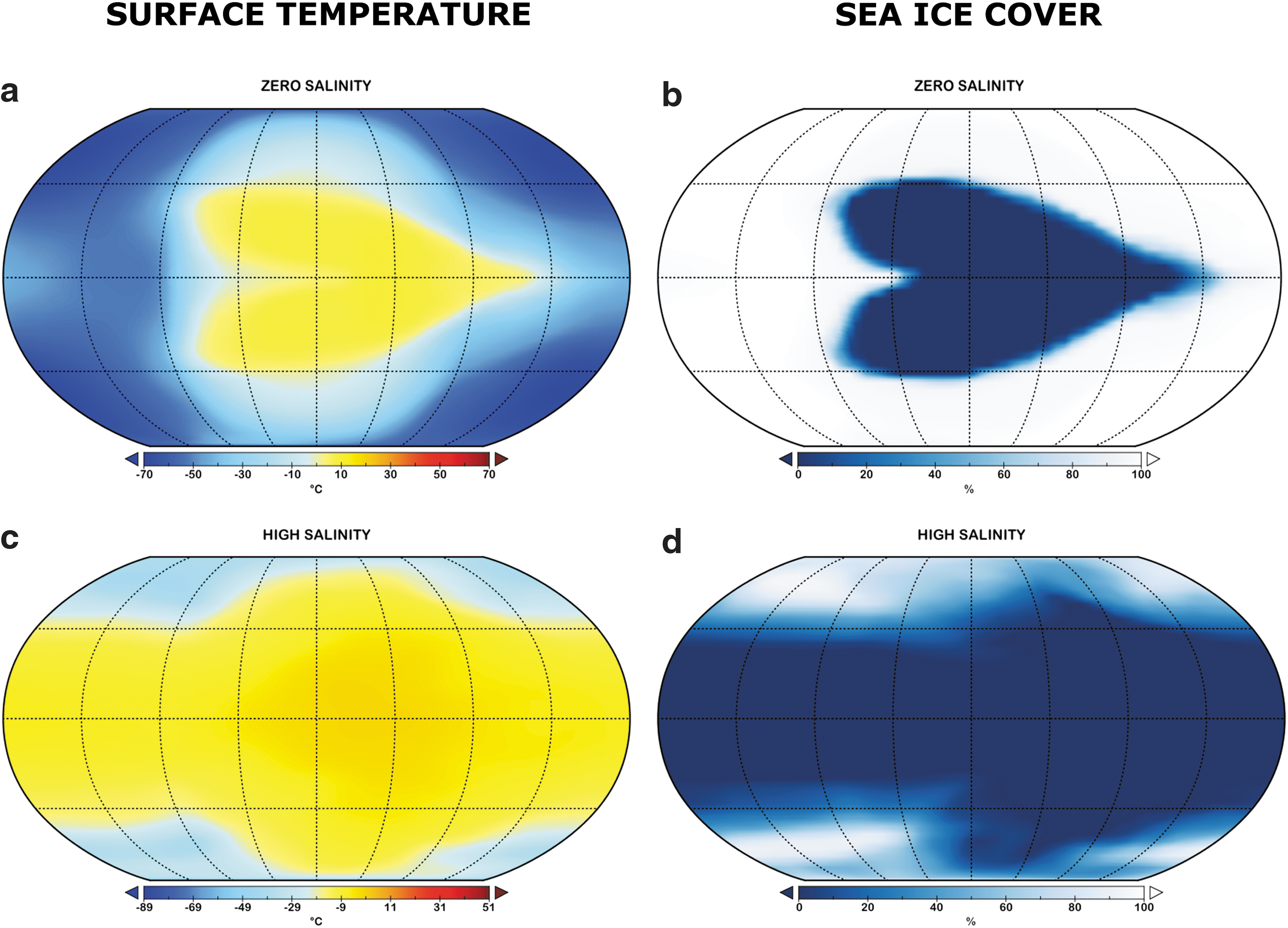
A wide range of Proxima b interior compositions are consistent with the observational constraint on its mass, including a significant water mass underlain by high-pressure ices and a negligible water mass fraction with a partly silicate mantle below (Brugger et al., 2016). Given our lack of knowledge of how much water was originally delivered to Proxima b, the nature of its source, and the history of its escape, an ocean-covered Proxima b could have a wide range of salinities. As discussed by Cullum et al. (2016), this has two implications for climate: (1) changes in the density-driven thermohaline ocean circulation and thus ocean heat transport, and (2) changes in the freezing point depression of seawater and thus the temperature threshold for surface liquid water.
Our experiments Zero Salinity (S = 0 psu) and High Salinity (S = 230 psu), patterned loosely after the work of Cullum et al. (2016), test this effect. For S = 0, the freezing point of seawater is 0°C (as opposed to −1.9°C in Control, for which S = 35.4), while for S = 230 psu seawater freezes at −19°C, several degrees warmer than the eutectic point temperature. The ocean model in ROCKE-3D uses an equation of state (Fotonoff and Millard, 1983) intended for Earth's ocean and linearly extrapolates the density of seawater for S > 40 psu, including the pressure dependence of the thermal expansion and haline contraction coefficients. At our coldest realized upper ocean temperature of −12.6°C (at which the local S = 232.8 psu) in High Salinity, this equation of state predicts a seawater density of ∼1230 kg/m3. By comparison, Sharqawy et al. (2010) presented a polynomial fit for seawater density at atmospheric pressure valid to within 0.1% up to S = 160 psu and down to 0°C; extrapolating to 232.8 psu and −12.6°C gives a density of 1192 kg/m3, 3% less than ROCKE-3D. Our primary interest, though, is the effect of the depression of the freezing point rather than the details of the ocean circulation.
Figure 9 shows surface temperature and sea ice cover for Zero Salinity and High Salinity. Compared with Control, the spatial patterns of warm temperatures and open ocean are very different: In Zero Salinity, the “lobster” has no extended tail, producing a less asymmetric pattern about the substellar longitude. In High Salinity, broad regions of open ocean extend into the extratropics, with only a weak remnant of the lobster pattern. More important for habitability is that the peak dayside temperature for Zero Salinity (High Salinity) is 7°C warmer (3°C colder) than Control, although the global mean temperatures are colder (warmer), respectively. The effects on sea ice cover and thus fractional planet habitability are more dramatic, with 10% less ice-free surface area in Zero Salinity (f hab = 0.32) and an almost ice-free planet (f hab = 0.87) in High Salinity despite surface temperatures on the latter planet that never exceed 0°C. The difference in remotely detectable equilibrium temperature between these two extreme planet scenarios, though, is only 6°C (Table 5).
As in Figure 8 but for experiments
In all three simulations, surface downwelling occurs in a narrow band near and upstream of the substellar point where the wind-driven circulation associated with the Rossby gyres converges; upwelling is concentrated in a narrow equatorial band east of the substellar region. In Zero Salinity, salinity forcing of the density-driven circulation (due to regional imbalances between surface evaporation E and precipitation P) is absent, and peak surface ocean current velocities are about half those in Control. The primary density-driven circulation is downwelling near the sea ice margins, due to the unique property of fresh water that its density peaks at 4°C. The equatorial westerly current seen in Control is almost absent in Zero Salinity except in the substellar region; most horizontal ocean heat transport takes place in the wind-driven subtropical gyres.
In High Salinity, nearly ice-free conditions are due primarily to the freezing point depression of the very salty water. The Rossby–Kelvin wave surface wind circulation still exists and produces surface ocean current convergence and downwelling of the ocean circulation at the equator, but the primary westerly surface ocean current extends to midlatitudes upstream of the substellar point. This is associated with an equator–pole density gradient that occurs upstream of the substellar region near the ocean surface but becomes almost zonal at depth, with cold, saltier water in the polar regions.
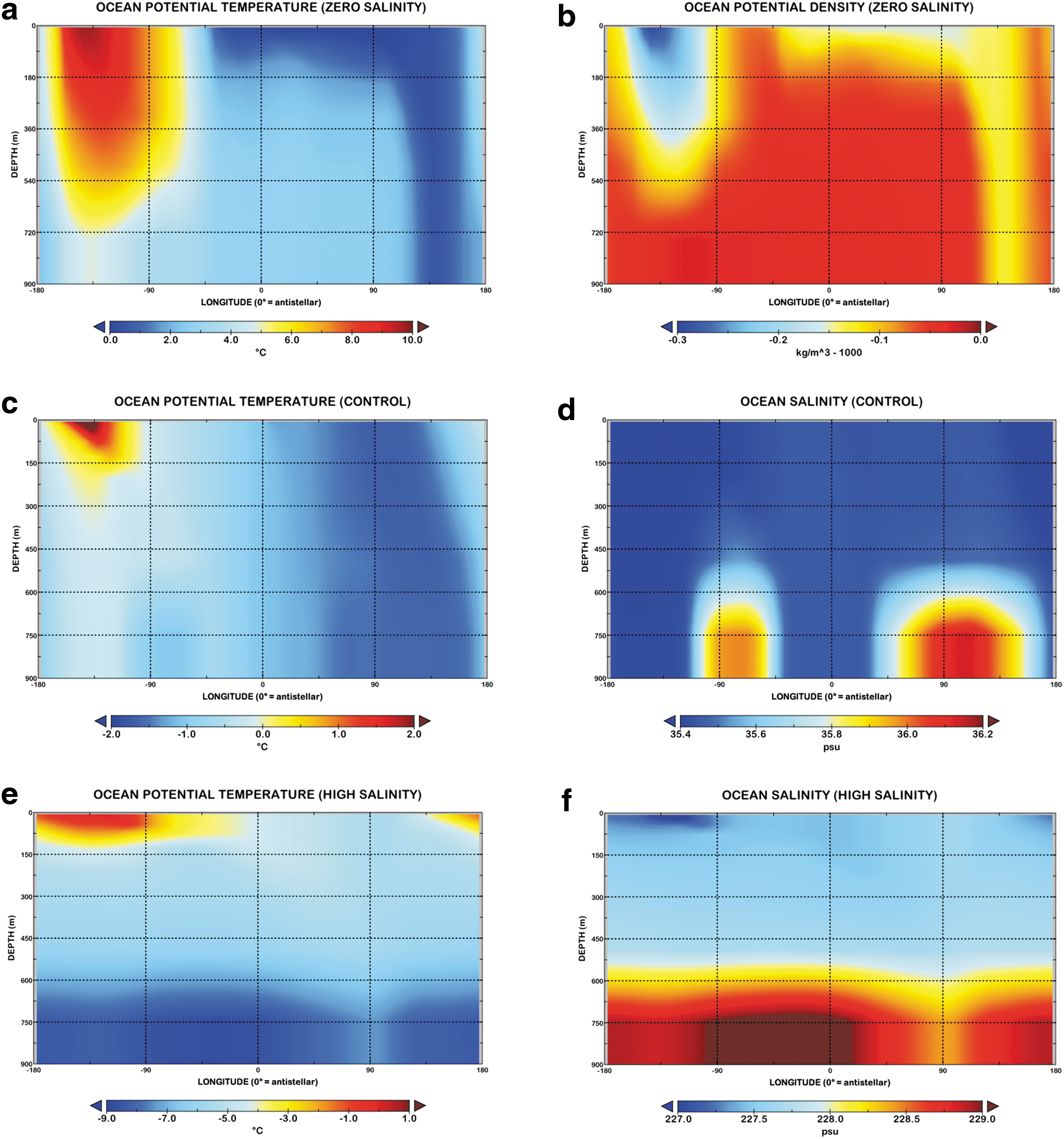
Figure 10 shows the ocean vertical structure along the equator for the three experiments with different salinities. In Zero Salinity, stratification is due to temperature differences alone (Fig. 10a), so the potential density structure (Fig. 10b) resembles that of potential temperature. For Control and High Salinity, potential density is controlled mostly by salinity differences, so we show the salinity structure instead. In Zero Salinity the ocean near and downstream of the substellar point is warm and stably stratified (potential density increasing downward), more weakly stratified on the nightside, and almost neutrally stratified upstream of the substellar point (Fig. 10a, b). In Control, warm water is more concentrated near the ocean surface downstream of the substellar point (Fig. 10c), with vertically uniform salinity there (Fig. 10d). In both Control and High Salinity, salty water collects at the bottom near both terminators, with fresher (i.e., lower salinity) water near the substellar and antistellar points. The salty water is due to sea ice formation, brine rejection, and downwelling of the resulting dense salty water at the sea ice margins at ∼10–30° latitude, which spreads toward the equator. This is interrupted, though, in the substellar and antistellar convergence regions where P > E and the water that sinks is fresher than elsewhere. The longitudinal contrasts in bottom water salinity are smaller in High Salinity because its more uniform surface temperatures produce weaker P–E differences.
Depth-longitude profiles at the equator of
Figure 11 compares the atmosphere and ocean heat transports in Zero Salinity and High Salinity with those in Control. Zero Salinity has the weakest and most tropically confined ocean transport of the three simulations but partly compensates with stronger atmospheric transports. High Salinity is just the opposite, with very weak atmospheric transport and stronger, more broadly distributed ocean transports. The total transports are nonetheless very similar to those in Control.
3.6. 3:2 spin–orbit resonance aquaplanets
As pointed out by Ribas et al. (2016), Proxima b may be in a 3:2 spin–orbit resonance rather than synchronous rotation. We conducted two experiments to explore the habitability of such states. The first (3:2e0) assumes eccentricity e = 0. This is done only for comparison with the work of Turbet et al. (2016), since a 3:2 resonance requires nonzero eccentricity (Goldreich and Peale, 1966; Ribas et al., 2016). The second (3:2e30) assumes e = 0.30, between the most likely estimate of e = 0.25 (Brown, 2017) and the upper limit of e = 0.35 (Anglada-Escudé et al., 2016).
Figure 12 shows incident SW radiation at the top of the atmosphere, surface temperature, and sea ice cover for these simulations. For e = 0, all longitudes receive the same time-mean instellation (Fig. 1 2a). The resulting atmospheric circulation is similar to that of a moderately slowly rotating Earth (Del Genio and Suozzo, 1987), with a Hadley cell in each hemisphere that extends most of the way to the pole, rather than the day–night circulation of synchronously rotating planets. This produces upper level westerly jets in midlatitudes and easterly trade winds at low latitudes in the near-surface Hadley cell return flow but a very weak westerly equatorial surface ocean current.
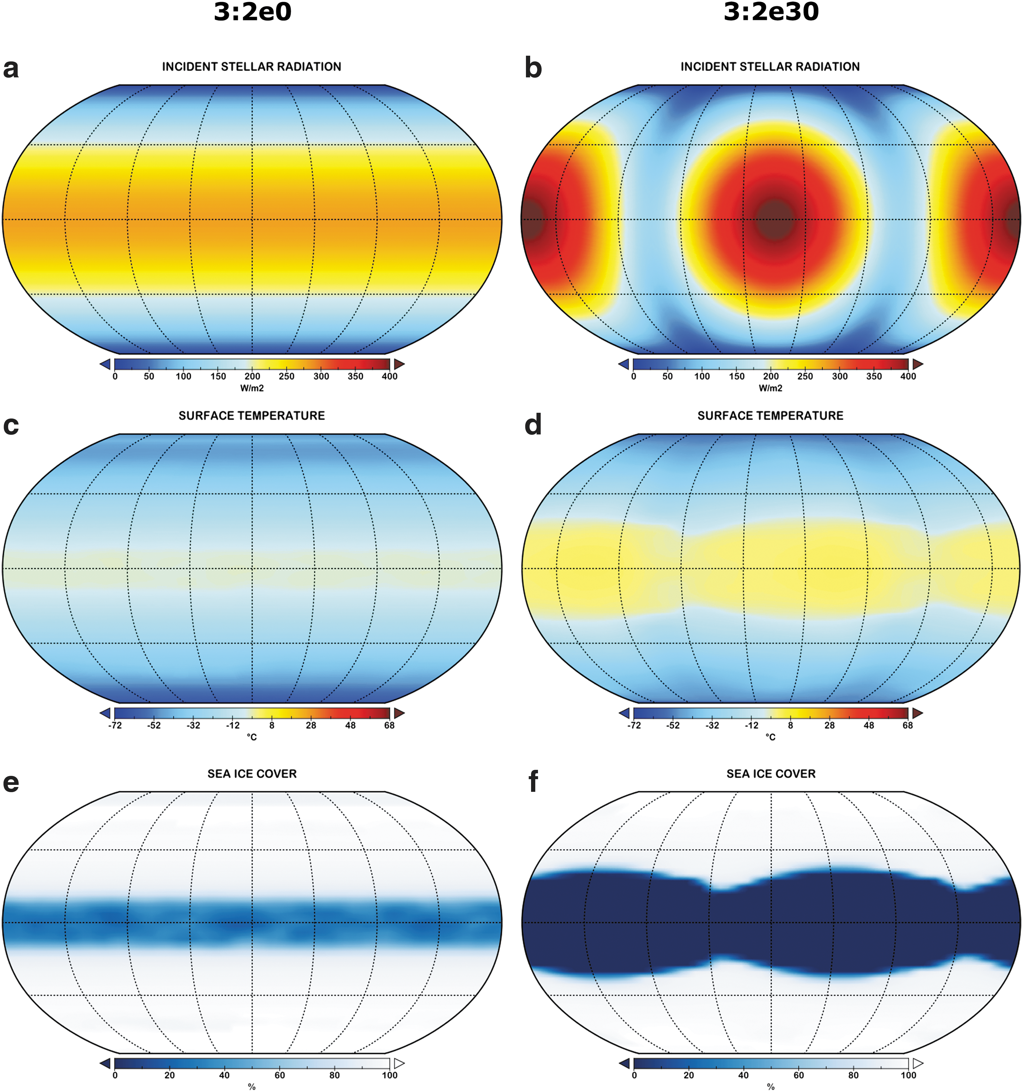
In 3:2 resonance, for which the rotation period is 7.5 days, the stellar day is 22.4 days, much shorter than the several Earth-year thermal response times of the 900 m ocean. This prevents thick sea ice from building up at low latitudes where instellation is greatest. But the thin (12 m) first ocean layer is able to partially freeze at night, with ∼20–30% sea ice cover (Fig. 1 2e) of 0.2–0.3 m thickness and otherwise open ocean with sea surface temperature at the freezing point near the equator in the time mean (although the surface air temperature is several degrees colder, Fig. 1 2c). This planet has the smallest liquid water area (f hab = 0.21) of all our dynamic ocean scenarios. Our result is fairly similar to that reported by Turbet et al. (2016), but theirs is achieved with an instellation 74 W/m2 higher than ours. Boutle et al. (2017) obtained an equatorial waterbelt using the same instellation we use, but only when they assumed a dark surface albedo; with a brighter albedo, their model produces transient open ocean conditions.
Of more interest is nonzero eccentricity, which is much more likely for an asynchronously rotating planet. In this case the stellar heating pattern has two maxima on opposite sides of the planet and weak heating at longitudes in between (Fig. 1 2b), as shown by Dobrovolskis (2007) and Brown et al. (2014). In the Boutle et al. (2017) model this leads to “eyeball” liquid water regions on either side of the planet and ice in between. In our simulations, though, the tropical ocean remains above freezing with no sea ice even at weakly irradiated longitudes that receive only 133 W/m2 instellation in the time mean (Fig. 1 2d). This climate is reminiscent of past “slushball” periods on Earth (Sohl and Chandler, 2007). The Proxima b tropical waterbelt however is zonally asymmetric (Fig. 1 2d), retaining some memory of the preferentially heated longitudes. Peak open ocean occurs slightly downstream of peak instellation due to weak eastward ocean heat transport at the most strongly heated longitudes. In fact atmosphere and ocean heat transports in both the meridional and zonal directions are weaker in 3:2e30 than in most other simulations (Fig. 11). This planet has somewhat larger liquid water area (f hab = 0.51) than the synchronously rotating Control (f hab = 0.42). For both asynchronous planets, T max and T min in Table 5 refer to equatorial and polar temperatures rather than dayside and nightside.
3.7. Earth-like land–ocean planets
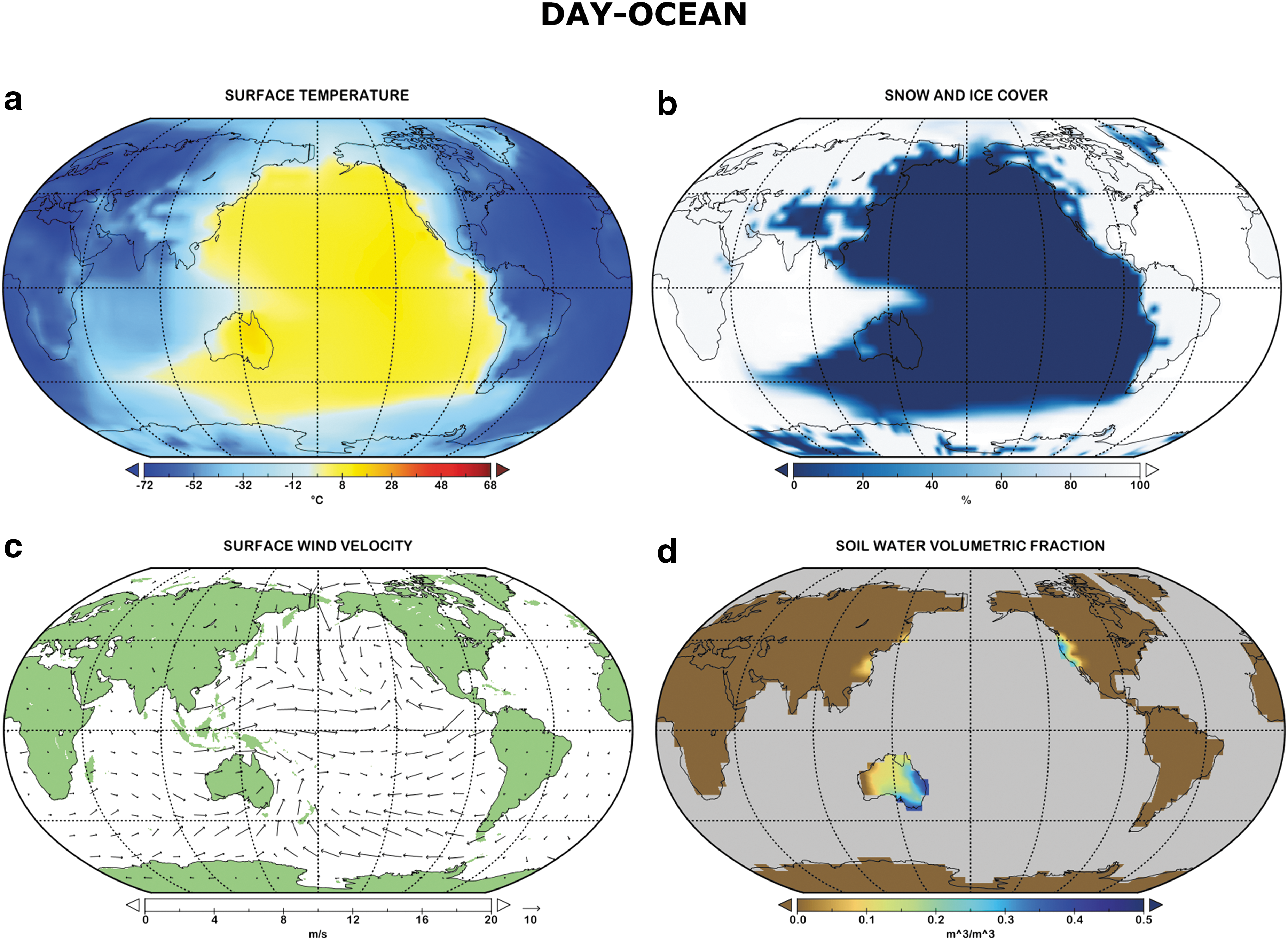
Moderate CO2 concentrations as assumed in most of our simulations may be more likely if some land is exposed to stabilize the climate through the carbonate–silicate cycle (Walker et al., 1981; Abbot et al., 2012). We conducted two experiments with synchronous rotation but modern Earth continents, differing only in substellar longitude. Experiment Day-Ocean places the substellar point at the dateline (180°), so that the strongest heating is over the Pacific Ocean. Day-Land has the substellar point at 30°E, over the African and Eurasian continents.
In many respects these two simulations most closely resemble our Thermo experiment, which ignores ocean heat transport (Table 5). Warm temperatures and surface liquid water (Figs. 13a, b and 14a, b) are restricted to the dayside in a pattern not too different from the eyeball Earth configuration of Thermo. The difference is that for Thermo, the eyeball pattern is produced artificially by excluding a process (ocean heat transport) that operates in nature. In Day-Ocean and Day-Land, it is due to the continental configuration of Earth, which is dominated by two large land masses oriented primarily north-south. This produces partly enclosed ocean basins that largely limit ocean heat transport to the nightside. In Day-Ocean, the southern hemisphere Rossby gyre advects heat around Australia, keeping some of the Indian Ocean ice free beyond the terminator. In Day-Land, the southern Rossby gyre is interrupted by South America, diverted south, and flows poleward through the Drake Passage, bringing warmer water to the coast of Antarctica that continues to flow westward and leaves a more significant nightside ice-free band adjacent to Antarctica.
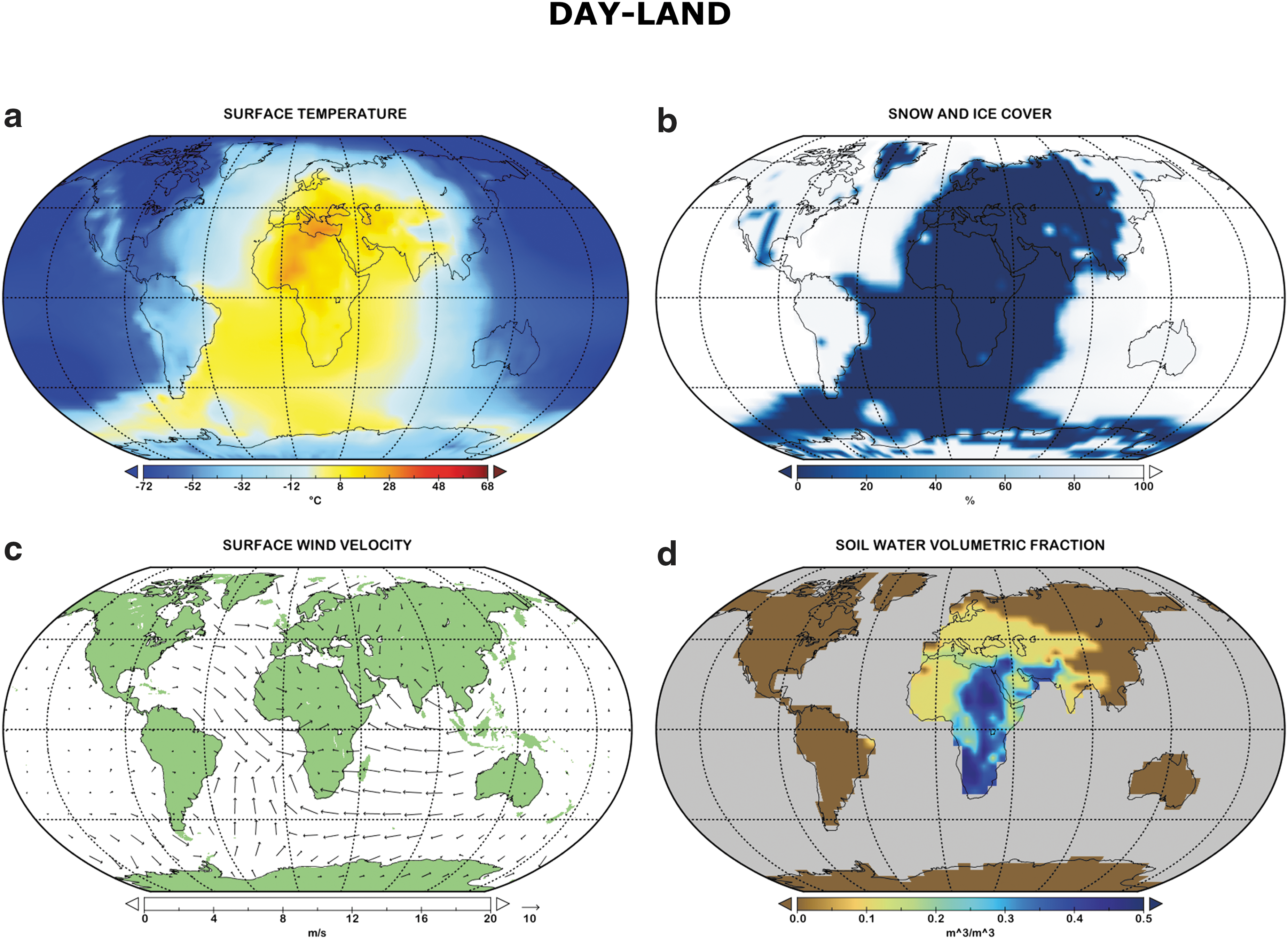
As in Figure 13 but for experiment Day-Land.
For Day-Ocean, zonal ocean transport is very weak relative to the aquaplanet experiments (Fig. 11), as expected, but this is compensated for by strong meridional ocean and atmosphere heat transport, as well as strong atmospheric zonal heat transport. Atmospheric transport in the southern hemisphere in fact more than compensates, giving a total transport in that hemisphere that is larger than most other experiments.
The Day-Ocean and Day-Land climates and circulations bear some resemblance to terrestrial winter and summer monsoons, respectively. In Day-Ocean, the near-surface flow (Fig. 13c) is generally directed offshore toward the central Pacific instellation peak, where convergence (and heavy precipitation, not shown) occurs in several bands determined partly by the influence of the Rossby–Kelvin wave pattern and partly by details of the continental distribution. In Day-Land, the flow is primarily onshore toward the African continent (Fig. 14c), where convergence and heavy precipitation occur. Subsurface liquid water reservoir levels (Fig. 14d, volume liquid soil water per volume of soil), an indicator of land surface habitability, are highest in Day-Land in a band where the near-surface convergence occurs. Areas with >0.3 volumetric fraction (0.4855 m3/m3 is the saturation value for our assumed soil mix and depth) are comparable with the wettest, most heavily vegetated places on Earth. This is surrounded by a broader dayside continental region where subsurface water volumetric fractions are 0.10–0.15, typical of annual means for semiarid to arid terrestrial climates. In Day-Ocean, the only habitable land areas are in coastal regions between the substellar longitude and the terminators (Fig. 13d) that are moderately wet, despite being far from the mid-Pacific convergence zone (Fig. 13c).
Elsewhere in Day-Ocean and Day-Land, land is snow covered. After 15,000 orbits (460 Earth years), net radiation, surface temperature, and planetary albedo have reached equilibrium. Snow depth artificially reaches equilibrium because the model places an upper limit on snow accumulation and returns any excess to the ocean. Yang et al. (2014) estimated from an offline land ice model that for a planet similar to ours, ice sheets of O (1 km) thickness should form on the nightside, though dayside water would remain for an inventory > ∼10% of Earth's oceans. Thus, we might expect the ocean in Day-Ocean and Day-Land to partly but not completely migrate to the nightside if ROCKE-3D could run to complete water cycle equilibrium (which would require tens of thousands of years or more, well beyond the capabilities of GCMs).
4. Discussion and Conclusions
We have shown that with a dynamic ocean, a hypothetical ocean-covered Proxima Centauri b with an atmosphere similar to modern Earth's can have a habitable climate with a broad region of open ocean, extending to the nightside at low latitudes. This is true for both synchronous rotation and a 3:2 spin–orbit resonance with moderate eccentricity. Because of its weak instellation, however, Proxima Centauri b's climate is unlikely to resemble modern Earth's. “Slushball” episodes in Earth's distant past with cold but above-freezing tropical oceans (Sohl and Chandler, 2007) are better analogues. The extent of open ocean depends on the salinity assumed. Moderately elevated greenhouse gas concentrations produce some additional warming, but this is limited for any M-star planet by the reduced penetration of near-IR starlight to the surface, and for Proxima b in particular, by its existence near a possible dynamical regime transition. “Eyeball Earth” scenarios with a warm substellar region do not occur in reality because of ocean heat transport, unless exposed land that creates a partially enclosed dayside ocean basin is present. We consider further implications of our results below.
4.1. Implications for the habitable zone concept
The nominal equilibrium temperature reported by exoplanet observers [e.g., by Anglada-Escudé et al. (2016) for Proxima b] and used to define the habitable zone is based on instellation and an assumed Earth-like planetary (Bond) albedo of 0.3. This is an unreliable indicator of habitability, since albedo and eccentricity vary among planets (Barnes et al., 2015), and planetary albedo varies with stellar spectral type (Kopparapu et al., 2013). The nominal equilibrium temperature (228 K) is identical in all our experiments except Control-High, yet mean (maximum) surface temperatures vary among the experiments by 47 (34) °C, and the ice/snow-free fraction of the surface varies from 0.20 to 1.0, largely because planetary albedo varies from 0.161 to 0.310 (Table 5). Only one of our simulations (Control-Thin) reaches the 0.3 Earth value of planetary albedo, because of absorption of the enhanced near-IR incident starlight by greenhouse gases and the reduced Rayleigh scattering of the atmosphere, as found in previous studies of M-star planets (Kasting et al., 1993; Kopparapu et al., 2013; Shields et al., 2013; Rugheimer et al., 2015).
The actual planetary equilibrium temperature (determined by the absorbed stellar flux), however, is a moderately good predictor of surface temperature in our N2- or CO2-dominated atmospheres, even though it is determined by emission primarily from the midtroposphere—there is a 0.41 correlation (significant at the ∼0.05 level) between T eq and T mean in Table 5. Thus, constraints on Bond albedo, for example, from SW phase curves, combined with knowledge of incident stellar flux, would be of some help in identifying a subset of promising planets from a large statistical sample of detected planet candidates for further study. The primary limitation of T eq is that it is relatively insensitive to variations in greenhouse gas amounts that can produce large differences in T surf. We return to this question in the next section.
Our High Salinity planet does not fit the traditional notion of habitability, since its time mean surface temperature never exceeds 0°C anywhere. Nonetheless, bodies of water on Earth such as the Dead Sea with conditions near 230 psu salinity are extensively inhabited by halophilic life (e.g., Fendrihan et al., 2006). Although these examples are at warm temperatures, Mykytczuk et al. (2012, 2013) reported that the bacterium Planococcus halocryophilus strain Or1 grows and divides in 180 psu water at temperatures as low as −15°C, not far from the ocean conditions in High Salinity, and is metabolically active down to −25°C.
The lower temperature limit of life is not yet defined (De Maayer et al., 2014). Standard cryopreservation temperatures for microbial cultures can be as low as −196°C in a cryoprotectant to maintain viable if not active cultures (Kirsop and Doyle, 1991). In nature, psychrophilic (or cryophilic) organisms have been observed to support metabolic functions in a hypersaline Antarctic spring as low as −20°C at 220–260 psu (Lamarche-Gagnon et al., 2015). All of the domains of life (Archaea, Bacteria, and Eucaryo) include halotolerant, halophilic, and haloextremophiles able to live or requiring environments with a range of salinities. These range through freshwater/seawater interfaces, typical seawater at 35 psu, and up to 359 psu at NaCl saturation, from extreme cold to hot temperatures (Oren, 2002).
Thus, if we think more broadly about what constitutes a habitable planet (Cullum et al., 2016), it is reasonable to imagine a cold but inhabited Proxima Centauri b with a very salty shallow remnant of an earlier extensive ocean in which halophilic bacteria are the dominant life-form, especially if the ocean is in contact with a silicate seafloor (Glein and Shock, 2010). We note that Jupiter's moon Europa, an object of interest in the search for life in our solar system, may have an ocean nearly saturated with salt (Hand and Chyba, 2007). Objects with subsurface oceans such as Europa and Saturn's moon Enceladus have been considered irrelevant to the search for life in other stellar systems because of the challenge of remotely detecting subsurface life, but they may be a useful analogue for water-rich, weakly irradiated tidally locked exoplanets that maintain a small region of substellar or equatorial surface liquid water that may be detectable.
Abbot et al. (2012) argued that an aquaplanet cannot support a carbonate–silicate cycle to stabilize climate, because the seafloor is insufficiently exposed to the temperature changes needed for weathering feedbacks. However, Charnay et al. (2017) found seafloor weathering to be an effective control on CO2 in Archean Earth simulations. The CO2 cycle has an unstable feedback due to temperature-dependent ocean dissolution of CO2 (Kitzmann et al., 2015; Levi et al., 2017). 3-D processes might counteract such tendencies if increased solubility in cold ocean regions offsets the effect of decreased solubility in the substellar region, with recycling following transport of colder ocean water back to the substellar region. Simulating the pattern of CO2 transport in a coupled ocean-atmosphere model and identifying the instellation and stellar temperature required for a stable cycle would help constrain long-term prospects for life on planets such as Proxima b.
SW radiation incident on the ocean surface in ROCKE-3D penetrates beneath the ocean surface to much shallower depths in the red/near-IR than at shorter wavelengths, but the partitioning in the model does not recognize changes in stellar spectrum. To test the sensitivity to the spectrum we performed a variation on Control attenuating the entire Proxima Centauri spectrum with the 1.5 m e-folding depth used for the red/near-IR, since 99.4% of the star's SW is in the red/near-IR versus 40% for the Sun. Because of the small amount of starlight reaching the ocean surface and the 12 m thickness of our first ocean layer, global mean surface temperature is within a degree of Control. Local deviations can be larger but only on the nightside. Subsurface temperatures are within 0.3°C almost everywhere. Local increases/decreases of sea ice cover of a few percent occur along the sea ice margin. Despite this, the impact on life underwater could be dramatic. The photic zone where photosynthetic life could be supported, assuming useful radiation at 400–1100 nm and a photon flux cutoff similar to the low-light limit in the Black Sea (Overmann et al., 1992), is effectively <10 m in this experiment versus 80 m on Earth, and even shallower at higher zenith angle.
4.2. The role of clouds
Terrestrial GCMs are traditionally categorized by their climate sensitivity; that is, the change in surface temperature per unit change in external radiative forcing (e.g., a change in greenhouse gas concentrations or insolation). For most models, the sensitivity lies in the range ∼0.5–1.5°C-m2/W (Andrews et al., 2012).
Following the work of Boutle et al. (2017), we estimate Proxima b climate sensitivity by comparing Control and Control-High. The latter has 18.6 W/m2 more global mean instellation and its mean surface temperature is 8°C warmer, yielding a climate sensitivity of 0.53°C-m2/W given the 0.234 Bond albedo of Control. This is greater than the ∼0.27°C-m2/W sensitivity found by Boutle et al. (2017) for a model with the same radiation scheme but different parameterizations of clouds, convection, and surface albedo, but similar to the ∼0.6°cm2/W sensitivity of our parent Earth GCM to a doubling of CO2 (Schmidt et al., 2014).
Boutle et al. (2017) suggested that low sensitivity occurs for a synchronously rotating planet because low-level clouds occur primarily on the nightside and do not affect reflected sunlight. Low clouds generally decrease in response to warming in Earth climate change simulations (Zelinka et al., 2016), decreasing planetary albedo and creating a positive feedback. A simple although imperfect measure of the effect of clouds on climate is the cloud radiative forcing (CRF), defined as the difference in SW and LW radiative flux with versus without clouds, the latter calculated offline in parallel with the actual model integration. Positive CRF means that the planet is warmer with clouds than without them. Thus usually SWCRF <0 because clouds are brighter than most planet surfaces, while LWCRF >0 because most clouds have a greenhouse effect.
In Control, the planet is nearly overcast (Fig. 15a). The nightside has almost ubiquitous low cloud (Fig. 15b), similar to the findings of Boutle et al. (2017), and has moderate to large middle (Fig. 15c) and high (Fig. 15d) cloud cover as well, but these are optically thin (vertically integrated liquid + ice water contents <40 g/m2 everywhere and <5 g/m2 in most locations). On the dayside, however, optically thick clouds (integrated ice+liquid water contents of 100–300 g/m2) generated by moist convection and large-scale upwelling in response to the direct stellar heating occur, as predicted by Yang et al. (2013) and other GCM studies for synchronously rotating planets. The dayside has >90% cloud fraction everywhere except for a small region near the low latitude morning terminator, where cloudiness is closer to 80%. Small clear to partly cloudy regions do occur occasionally on timescales of an orbit or more, but primarily near the terminators and at high latitudes. If this is typical of synchronously rotating exoplanets with extensive surface oceans, detection of surface biosignatures or even the ocean itself will be difficult. Analysis of the stochastic properties of these clouds would be needed to quantify the detectability of such features from different viewing angles and phases as may be observed by future direct imaging missions.

Control
Figure 16 shows the response of these clouds to the instellation increase from Control to Control-High. Increased instellation produces regional increases and decreases in low-cloud fraction (Fig. 16a) but no systematic day or night change. High-cloud fraction increases weakly in the substellar region and to a greater extent in the equatorial region on the nightside (Fig. 16b). More important is the dayside strengthening (i.e., becoming more negative) of SWCRF (Fig. 16e). This appears to be due partly to increasing cloud optical thickness associated with an increase in cloud water path, much of it in high ice clouds but some in the liquid phase in lower altitude clouds as well (Fig. 16c, d). This results in a more negative SWCRF there; that is, a negative SW cloud feedback over the dark substellar ocean. Significant increases in LWCRF also occur on both the dayside and nightside over open ocean; this may slightly underestimate the true LW cloud feedback since the cloud forcing approach conflates the effects of cloud changes with collocated noncloud feedbacks (Soden et al., 2004).

Changes in
Table 7 shows global mean and dayside maximum values of SWCRF and LWCRF, as well as the global mean clear-sky greenhouse effect <Ga > = <σTsurf 4 > – <σTeq 4 > – <LWCRF> (where the brackets indicate that the fluxes are area averaged), for each simulation. In general, the warmer the peak substellar temperature T max, the stronger (more negative) SWCRF is, but this only explains part of the variance in SWCRF (correlation coefficient −0.69).
Maximum and Global Mean SWCRF and LWCRF, Ratio of Maximum LWCRF to −SWCRF (R), and Global Mean Clear-Sky Atmospheric Greenhouse Effect (G a) for Each Experiment
All fluxes are reported in W/m2.
LWCRF, longwave cloud radiative forcing; SWCRF, shortwave cloud radiative forcing.
<SWCRF> and <LWCRF> values for the experiments are uncorrelated with each other across our ensemble, but their maximum values in the substellar convection region are highly correlated (−0.74), as they are in tropical deep convective regions on Earth (Kiehl, 1994). Unlike Earth, however, where Kiehl (1994) found that SWCRF and LWCRF nearly offset each other (R = −LWCRF/SWCRF ∼ 1) to produce near-zero net cloud forcing in convective regions, substellar LWCRF is considerably smaller than SWCRF in our Proxima b simulations (R = 0.10–0.59, Table 7).
This appears to occur for several reasons: the day–night circulation in our synchronously rotating cases, the height of convective cloud systems, and noncondensing greenhouse gas concentrations. Unlike Earth's tropics, where thick high clouds are common but variable in time due to propagating disturbances and not strongly correlated with time of day, on a synchronously rotating planet such clouds are usually present and coincident with strong instellation. Consequently, peak SWCRF exceeds that on Earth. Second, the Proxima b convective clouds are not as deep as Earth's, because of the weak instellation relative to the peak daytime value that Earth receives from the Sun and the stronger near-IR absorption by H2O, CO2, and CH4 that stabilizes our Proxima b troposphere (Fig. 4). Especially low values (R = 0.10–0.19) occur for Pure CO2 and the three Archean simulations, which have among the weakest peak LWCRF (Table 7) due to the elevated greenhouse gas concentrations that reduce the opacity contrast between clear and cloudy sky.
Our synchronous rotation experiments support the nightside “radiator fin” analogy to Earth's subtropics discussed by Yang and Abbot (2014). The best predictor of nightside minimum surface temperature in our simulations is the clear-sky greenhouse effect Ga (correlation 0.94), which is much larger than LWCRF (Table 7). Although total day–night transport is relatively invariant across the ensemble, Ga is weak for experiments whose total heat transport (Figs. 6, 7, and 11) is slightly weaker than average (Thermo, Control-Thin, Zero Salinity, and Day-Ocean), all of which are quite cold on the nightside, whereas Control, Control-High, and High Salinity have slightly larger total transport, higher Ga values, and more moderate nightside climates. The warmest nightside conditions (in addition to High Salinity) are for Pure CO2 , Control-Thick, and several of the Archean simulations, due to those experiments' elevated CO2 and/or CH4 levels. The common thread linking all the experiments is that an optically thicker nightside atmosphere, whether due to evaporated or transported water vapor or to higher concentrations of spatially uniform noncondensing greenhouse gases, helps sustain warmer nightside temperatures.
A very strong correlation exists between f hab and <Ga > for synchronously rotating planets across our ensemble (0.87). The correlation between <Ga > and the difference ΔF between maximum and minimum emitted thermal radiation is almost as large (−0.78). For example, <Ga > = 52 W/m2 and ΔF = 118 W/m2 for Control, which has a modern Earth-like atmosphere, versus <Ga > = 186 W/m2 and ΔF = 24 W/m2 for Pure CO2 , which is more of an ancient Mars analogue. This suggests that the amplitude of flux variations in thermal phase curves can be used qualitatively to distinguish “maximum greenhouse”-type planets with thick atmospheres and higher surface temperature from more Earth-like planets. Given such information, T eq can potentially provide more useful inferences about T surf.
Our Zero Salinity and High Salinity simulations raise the question of how cloud particles are nucleated on exoplanets. On Earth, sea salt is a significant component of the aerosol and cloud condensation nucleus population over remote ocean areas, especially when strong surface winds are present. It is conceivable that exoplanet oceans with higher salinities than Earth's ocean might form somewhat brighter clouds than our or any GCM predicts due to greater sea salt availability, though this effect is probably secondary to dynamical and surface differences that influence cloud fraction. A more difficult question is how a planet like Zero Salinity would nucleate clouds at all, given the absence of continental sources of naturally occurring aerosol. Such a planet might require external sources of particles from meteoric debris or internally produced photochemical hazes to nucleate clouds, as probably occurs on several solar system planets.
4.3. Relevance to other known exoplanets
Our simulations are specific to best estimate parameters for Proxima Centauri b and assume an atmospheric composition, water inventory, and land/ocean distribution that are at present unknown, but the results should be at least qualitatively applicable to similar recently discovered potentially rocky planets orbiting other very cool M stars. For example, the TRAPPIST-1 system of planets (Gillon et al., 2017) orbits a star of temperature 2519 K (Van Grootel et al., 2017), about 500 K colder than Proxima Centauri. Similar concerns about water loss exist for this system as for Proxima Centauri b (Bolmont et al., 2017), but given the unknown evolutionary path of the system planets that retain water cannot be ruled out. One planet (TRAPPIST-1 e) is 0.918 times the radius of Earth, receives an incident stellar flux 0.662 times the flux incident on Earth, very close to that received by Proxima b, and has a synchronous rotation period of 6.1 days, slightly more than half that of Proxima b. Simulations of TRAPPIST-1 e by Wolf (2017) and Turbet et al. (2018) with a thermodynamic ocean aquaplanet and a 1 bar N2 atmosphere with a modest CO2 concentration yield a cold but partly habitable “eyeball” planet with mean surface temperature similar to our Thermo simulation. Thus, our Control simulation might be a useful analogue for this planet if it has an Earth-like atmosphere, or Pure CO2 if it is ancient Mars-like.
Astudillo-Defru et al. (2017) announced nine new nearby planets observed by the HARPS spectrograph. One of these (GJ 273 b) orbits a 3382 K M star, receives 1.06 times the solar flux received by Earth, is 2.89 or more times the mass of Earth, and has an orbital period of 18.6 days. If the actual mass is close to the minimum mass and/or the density is greater than Earth's, GJ 273 b could be a rocky planet. If so, the instellation and ΔF synchronous rotation values are close enough to those of our simulations for us to anticipate a GJ 273 b climate somewhat warmer than (and thus having more habitable surface area than) but otherwise similar to our Proxima b Control-High case, given the same type of atmosphere. [For example, Fujii et al. (2017) simulated substellar temperatures of ∼290–295 K for an Earth-sized planet with a static ocean orbiting the stars GJ 876 and Kepler-186, which are somewhat cooler and warmer, respectively, than GJ 273.] Another planet, GJ 3293 d, orbits a 3480 K star, receives 0.59 times the solar flux incident on Earth, has a minimum mass 7.6 times that of Earth, and orbits once every 48.1 days; depending on its actual mass and density, it may or may not be a rocky planet. If it is, its climate could be similar to those described here for Proxima b given a similar atmosphere, but it is more likely to be in the slowly rotating day–night dynamical regime than the Rossby–Kelvin regime.
Most recently, Dittman et al. (2017) reported a planet orbiting a 3131 K M star, LHS 1140 b, which is 1.4 times the radius and 6.6 times the mass of Earth, and receives 0.46 times the instellation that Earth receives. This level of stellar heating makes it marginal for habitability. Using a GCM with a static ocean, Fujii et al. (2017) found that for GJ 876, a star similar in temperature to LHS 1140, an Earth-sized planet with a 1 bar N2 atmosphere and a minimal amount of CO2 (1 ppmv) has a substellar surface temperature of ∼262 K (and is thus ice covered) for instellation 0.4 times Earth's; the temperature is ∼281 K for instellation 0.6 times Earth's. This suggests that with larger greenhouse gas concentrations more like our Archean High or Pure CO2 case and a dynamic ocean, scenarios may exist in which LHS 1140 b can be habitable, especially if any ocean is saltier than Earth's.
The population of potentially habitable rocky exoplanets in M star systems has now suddenly reached the point at which it will soon be possible to assess the demographics of this class of planet. Future research will benefit from the context provided by climate model studies of this class as a whole in anticipation of efforts to begin detecting and characterizing their atmospheres. Several such general GCM studies have already occurred (Bolmont et al., 2016; Kopparapu et al., 2016; Fujii et al., 2017; Wolf et al., 2017; Carone et al., 2018; Turbet et al., 2018), but exploration of the parameter space of factors that influence the climates of these planets has only just begun.
Footnotes
Acknowledgments
We are grateful to Andrew Lincowski, Giada Arney, Eddie Schwieterman, Jacob Lustig-Yeager, and Vikki Meadows of VPL, who created the Proxima Centauri stellar spectrum and generously shared it with us for this article. We thank Bill Kovari for assistance with figures. We also thank three reviewers for constructive comments that helped us improve the article. This work was supported by the NASA Astrobiology Program through collaborations arising from our participation in the Nexus for Exoplanet System Science, and by the NASA Planetary Atmospheres Program. Computing resources for this work were provided by the NASA High-End Computing (HEC) Program through the NASA Center for Climate Simulation (NCCS) at Goddard Space Flight Center.
Author Disclosure Statement
No competing financial interests exist.