Spatial Spectroscopic Models for Remote Exploration

Abstract

Ancient hydrothermal systems are a high-priority target for a future Mars sample return mission because they contain energy sources for microbes and can preserve organic materials (Farmer, 2000; MEPAG Next Decade Science Analysis Group, 2008; McLennan et al., 2012; Michalski et al., 2017). Characterizing these large, heterogeneous systems with a remote explorer is difficult due to communications bandwidth and latency; such a mission will require significant advances in spacecraft autonomy. Science autonomy uses intelligent sensor platforms that analyze data in real-time, setting measurement and downlink priorities to provide the best information toward investigation goals. Such automation must relate abstract science hypotheses to the measurable quantities available to the robot. This study captures these relationships by formalizing traditional “science traceability matrices” into probabilistic models. This permits experimental design techniques to optimize future measurements and maximize information value toward the investigation objectives, directing remote explorers that respond appropriately to new data. Such models are a rich new language for commanding informed robotic decision making in physically grounded terms. We apply these models to quantify the information content of different rover traverses providing profiling spectroscopy of Cuprite Hills, Nevada. We also develop two methods of representing spatial correlations using human-defined maps and remote sensing data. Model unit classifications are broadly consistent with prior maps of the site's alteration mineralogy, indicating that the model has successfully represented critical spatial and mineralogical relationships at Cuprite. Key Words: Autonomous science—Imaging spectroscopy—Alteration mineralogy—Field geology—Cuprite—AVIRIS-NG—Robotic exploration. Astrobiology 18, 934–954.

1. Introduction

Ancient hydrothermal systems are a high-priority target for a future Mars sample return mission because they contained energy sources for microbes and can preserve organic materials (Farmer, 2000; MEPAG Next Decade Science Analysis Group, 2008; McLennan et al., 2012; Michalski et al., 2017). Two candidate landing sites (Northeast Syrtis Major and Gusev Crater) for the Mars 2020 rover have evidence for alteration at elevated temperatures (Squyres et al., 2008; Bramble et al., 2017). Determining their fluid temperature, chemical composition, pH, Eh, and volume will be key to understanding both their habitability and biosignature preservation potential. Much of this knowledge is ascertained from the mineral assemblages and sequences of minerals that result from the hydrothermal circulation. However, these hydrothermal systems are difficult to explore remotely. They are often spatially heterogeneous and may only be visible at isolated surface locations across the area of interest. While a field geologist can investigate sites using as many field observations and laboratory analyses as necessary, a rover on another planet is more limited. Finite mission lifetimes and slow communications cadence reduce the amount of data that can be acquired, making effective time allocation critical to the overall science return. New operations models will be important for future planetary missions searching for biosignatures, seeking to understand whether environments were ever habitable, or collecting samples to return to Earth.

One promising solution is to engage the remote system as a more active participant in science data analysis. Historically, most missions have favored simple scriptlike measurement and action sequences that are transmitted to the remote explorer for rote execution (Fong, 2017). The robot completes the plan and transmits the resulting science data back for analysis and after some delay receives new commands. This is simple but inefficient; it often requires a day or more for each decision, limiting the finite mission's science yield. The failure of any one activity in the sequence costs additional time as the agent pauses and waits for new instructions. For many missions, downlink bandwidth accommodates a tiny fraction of the potential data (Jasper and Xaypraseuth, 2017). More flexible autonomy will be important to overcome these limits and enable critical emerging astrobiology investigations for outer planet exploration (Lorenz and Cabrol, 2018), high-volume instruments (Thompson et al., 2013, 2015a; Bekker et al., 2014), and wide-area adaptive sensing (Fink et al., 2005; McGuire et al., 2014; Woods et al., 2014). Such platforms must move beyond rote execution of command sequences to actively respond and adapt to the latest data in a more flexible collaboration with the operators.

A fundamental challenge of robotic science autonomy is encoding the best response to an infinite set of potential measurements. Prior science autonomy systems deployed to space, such as AEGIS (Estlin et al., 2012; Francis et al., 2017), EO-1 (Chien et al., 2005), and those in active development at the time of this writing (Thompson et al., 2015c; Doran et al., 2016), constrain the challenge by responding to specific triggers in instrument data. It is difficult to automate more fundamental autonomy based on abstract properties that are not directly measurable, such as geologic unit classifications.

Several aspects of abstract science interpretations are particularly challenging to encode. First, they often hinge on prior knowledge of the environment and preexisting remote sensing measurements (Thompson et al., 2015b). Second, human scientists continually reinterpret their measurements with a growing contextual knowledge of the environment; and, contrary to most artificial intelligence applications, real missions involve frequent reformulation of objectives throughout the investigation (Hock et al., 2007). Third, science decisions must consider complementary information from multiple sensing modalities and multiscale spatial relationships (Thompson et al., 2011).

These factors are all relevant for hydrothermal systems, since biosphere-relevant formation conditions are abstract geophysical processes that are far removed from the instrument data values available to the robot. Autonomous science decisions require a quantitative model relating hypotheses to instrument data, in order to calculate the information content. It is not typically feasible to encode rich scientific knowledge that would enable true robotic understanding. However, it is possible to describe statistical relationships between abstract hypotheses and measurable data (Thompson et al., 2011). This could drive principled experimental design decisions that adapt the measurement plan (Shewry and Wynn, 1987). Such models can relate collected data to the investigation questions without having to capture all the scientists' knowledge.

This article develops the approach with a case study involving remote in situ exploration of a hydrothermal system. The Cuprite Hills contain lithologies formed within active hydrothermal systems with a variety of fluid temperatures and compositions, and this site has been well characterized with both traditional geologic field methods and high spatial and spectral resolution remote sensing (Swayze et al., 2014), providing ground truth for this study. While we focus on a hydrothermally altered site, these methods are equally applicable to other sites where water was present, including paleolakes, deltas, and sites of low-temperature weathering, which could also have hosted and preserved life (McLennan et al., 2012).

We simulate a robotic spacecraft mission using three general sources of data: (1) geologic maps published from previous studies; (2) a broadband remote sensing system with capabilities similar to the Advanced Spaceborne Thermal Emission and Reflection Radiometer, ASTER (Rowan et al., 2003); and (3) an in situ robot with a profiling spectrometer measuring from 0.35 to 2.5 μm, the visible shortwave infrared (VSWIR) interval that captures diagnostic features of alteration minerals. We simulate the profiling spectrometer with traverses of data from NASA's Next Generation Airborne Visible/Infrared Imaging Spectrometer, AVIRIS-NG (Hamlin et al., 2011; Thompson et al., 2018). The high-resolution AVIRIS-NG data provides complete coverage of the site so that we can simulate any possible robot sampling strategy and path. For in situ robotic spectroscopy, we use Tetracorder analyses which identify the minerals and other materials found in each spectrum. Such an identification system could be employed on a rover, providing real-time materials identification. A probabilistic spatial model relates mineral identifications to investigation objectives, enabling adaptive information-driven exploration planning (Arora et al., 2017; Candela et al., 2017) while the robot is out of touch with operators. In the context of a human scientist and robotic explorer working together, this transforms the co-robotic relationship from one in which the scientist plots a path into a collaboration in which the human and robot work together to fill in gaps in knowledge and make discoveries.

2. Approach

The Cuprite Hills are located about 200 km northwest of Las Vegas, Nevada (Fig. 1). They show diverse relict hydrothermal alteration minerals formed over specific pH and temperature ranges. The surface minerals can indicate a range of geologic conditions and processes. Many passive remote sensing instruments can identify these minerals, making Cuprite an important test site for remote measurement algorithms. Studies began with the first broadband remote sensing instruments (Rowan et al., 1974; Abrams et al., 1977) and later included imaging spectrometers in the visible, shortwave, and thermal infrared regimes (Goetz and Srivastava, 1985; Kruse et al., 1990). This section describes our simulation of a remote surface investigation at Cuprite. We formalize exploration objectives using a statistical model with spatial extent. This defines the distribution of mineralogical information throughout the site and the information value of new measurement data with respect to science hypotheses.

FIG. 1.

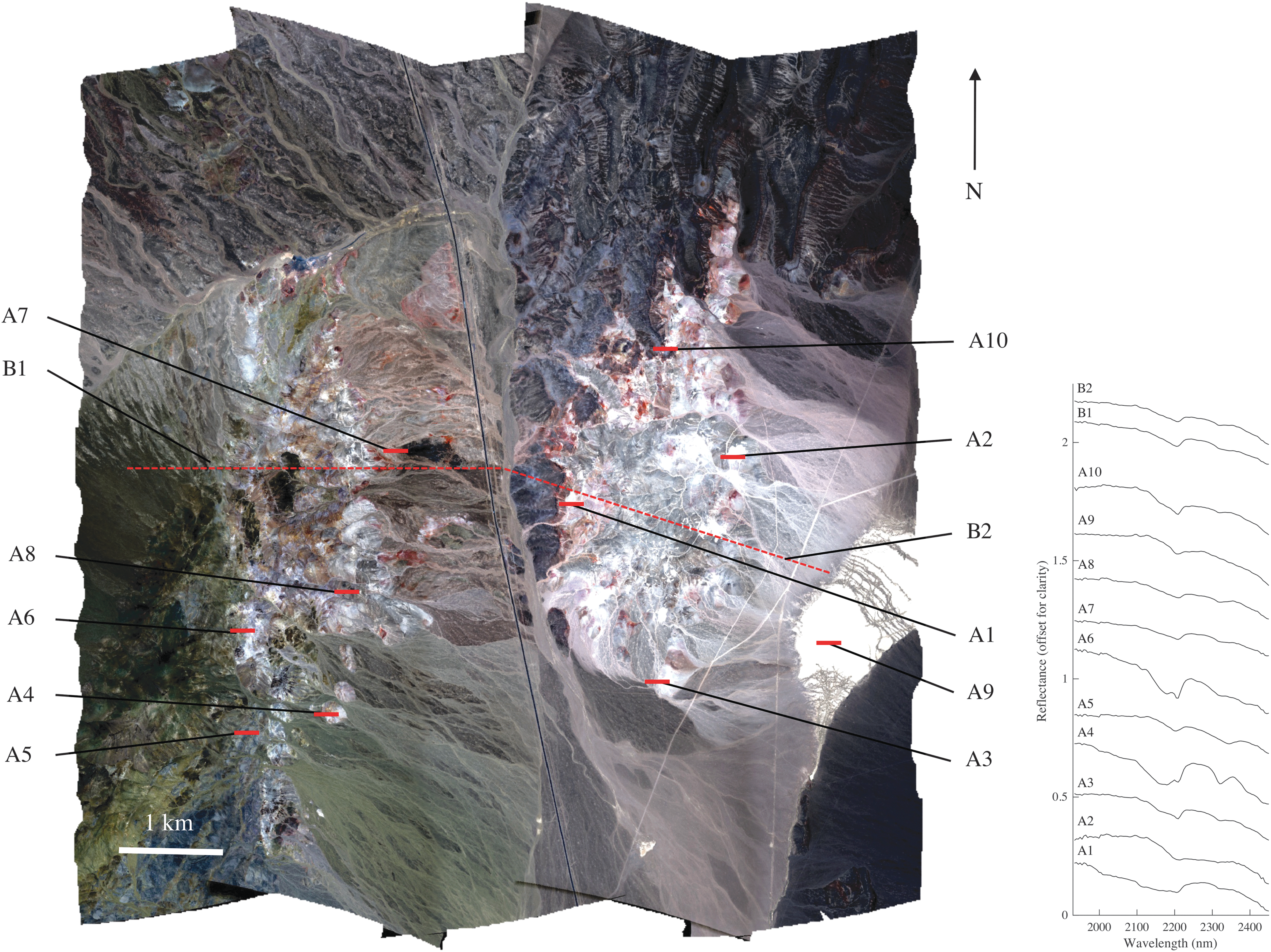
Left: Visible wavelength mosaic of Cuprite Hills, Nevada, as seen by the AVIRIS-NG sensor during an overflight in June 2014. Annotations indicate red lines showing transects of interest in Table 3. Right: Average reflectance spectra from each transect.

2.1. Science traceability

Conventionally, modern NASA missions use a Science Traceability Matrix (STM—Tables 1 and 2) to relate fundamental investigation questions to measurable physical quantities and thence to instrument requirements. Our case study uses a simple STM corresponding to investigation objectives, physical properties, and measurements. We consider two alternative missions with different objectives. Objective I emulates early reconnaissance on a planetary surface with little advance knowledge. Here, investigators seek a coarse geologic classification of the major surface units using broad classes such as Lacustrine, Metamorphic/Hydrothermal, Igneous, and so on. We begin with an overcomplete list including classes like Evaporitic that have not been observed at Cuprite (Swayze et al., 2014). Each of these originating processes is associated with one or more specific detectable minerals in the second column. Minerals are typically consistent with multiple geologic unit classifications, and vice versa. The third column shows measurements that can detect the minerals by using distinctive combination absorption features in surface reflectance from 2 to 2.5 μm (Kruse, 2009; Van Der Meer, 2004). Example signatures appear in the right panel of Fig. 1. These are average reflectance spectra drawn from reference transects A1–A10 and B1–B2, which we will reference throughout this study. Even these summary averages reveal clear differences in the spectral shape, indicating compositional variability or the presence of relevant minerals at small abundances (Swayze et al., 2014). Broadband instruments cannot resolve specific minerals in this manner, but they do indicate coarse differences in geologic units. Consequently, a multiband instrument with wide coverage could allow the mission to extrapolate in situ spectroscopic classifications over wide areas, though with a lower level of confidence than with direct spectroscopic measurements (Kruse et al., 2009; Thompson et al., 2013).

Table 1.

Science Traceability Matrix (STM) for Objective I: Broad Area Geologic Classification

Objective I	Physical properties	Measurements
Determine the dominant origin of major geologic units in Cuprite:	Presence of key minerals including	Remote surface reflectance, 450–2500 nm over 9 representative channels at 30 m spatial resolution and >300 signal-to-noise ratio (SNR)
1. Lacustrine/Marine	1. Alteration minerals
2. Evaporitic	2. Hydrated minerals
3. Metamorphic/Hydrothermal	3. Carbonates
4. Pedogenic/Diagenetic	4. Sulfates
5. Igneous	5. Phyllosilicates	In situ surface reflectance, 450–2500 nm at 10 nm spectral resolution and >300 SNR
6. Biogenic	6. Other
7. Other

Table 2.

Science Traceability Matrix (STM) for Objective II: Assessment of Alteration State

Objective II	Physical properties	Measurements
For each of the hydrothermally altered areas, determine the spectrally dominant Swayze (Swayze et al., 2014) alteration type:	Presence of alteration minerals including
	1. Chalcedony
	2. Opal	Remote surface reflectance, 450–2500 nm over 9 representative channels at 30 m spatial resolution and >300 signal-to-noise ratio (SNR)
	3. Alunites
	4. Dickite
	5. Well-ordered Kaolinite
1. Silica	6. Halloysite
2. Alunite	7. White Mica
3. Kaolinite	8. Chlorite
4. White Mica ± Montorillonite	9. Buddingtonite ± Smectite	In situ surface reflectance, 450–2500 nm at 10 nm spectral resolution and >300 SNR
5. Chlorite	10. Hematite
6. Adularia-smectite	11. Jarosite
	12. Goethite
	13. Others

Table 2 describes our second objective, an in-depth investigation of hydrothermally altered regions. The alteration scale of Swayze et al. (2014) associates alteration zones at Cuprite with the presence of one or more detectable minerals. These alteration zones represent different regimes of temperature, pressure, and pH, linking Cuprite's mineralogy to two overlapping hydrothermal systems: (1) an earlier adularia-sericite system where buddingtonite is found and (2) a later overprinting advanced argillic system. The younger system is most widespread in the eastern center. Erosion is greater in the western center and exposes more of the adularia-sericite alteration. Here we use the alteration scale of Swayze et al. (2014) as an intermediate classification that captures the relevant zones of alteration minerals present on the surface and directly visible to spectroscopy. Some minerals indicate very specific alteration zones; for example, chlorite is spectrally dominant in the zone that bears its name and uniquely identifies it. In contrast, other minerals like jarosite appear in many alteration zones. The names of the zones generally indicate the spectrally dominant minerals. While Objective II is more refined than Objective I, the measurement strategy is similar. Wide-area multiband images of the site can delineate different unit areas, while small-scale surface spectroscopy can detect specific minerals.

2.2. Geospatial data sets

We use a probabilistic map as a structure in which human scientists initially describe their understanding about the world and in which the understanding evolves as the robotic explorer collects information. These maps represent hypothesized arrangements and classifications of properties of an environment with corresponding probabilities. This expressive representation captures spatial structure at many scales, with the potential to incorporate categorical, continuous, and multivariate data. Maps are intuitive and close to the way that working hypotheses are already expressed in Earth and planetary exploration (Wray et al., 2009; Milliken et al., 2010). Robots can use them as a guide to explore efficiently without the tedium of operator micromanagement or the need for low-latency communications. By focusing on maps as a medium for both data understanding and planning, we play to the advantages of both human (domain expertise) and robot (formal optimality and immediate responses to new data).

Geologic maps represent spatial relationships—the correlations between measurements, minerals, and geologic classes at different locations and scales. We consider two formulations that could capture these relationships to estimate complete maps from point measurements. The first strategy, which we will call partitioning, ascribes geologic classifications to contiguous predefined spatial units. Measurements within each partition are treated as Independent, Identically Distributed (IID) draws from a common underlying distribution. Consequently, the measurements within each predefined partition all contribute equally to the common classification. The second strategy, which we will call remote sensing, uses the natural correlations across spatial locations that appear in wide-area remote measurement data. Remote sensing reveals spatially continuous properties of the environment. A mission can incorporate this data into the model as an additional observable and learn to interpret it during exploration by assimilating the in situ data as a reference. The resulting maps will be spatially smooth; nearby locations will generally have similar remote measurements and as a consequence similar classifications.

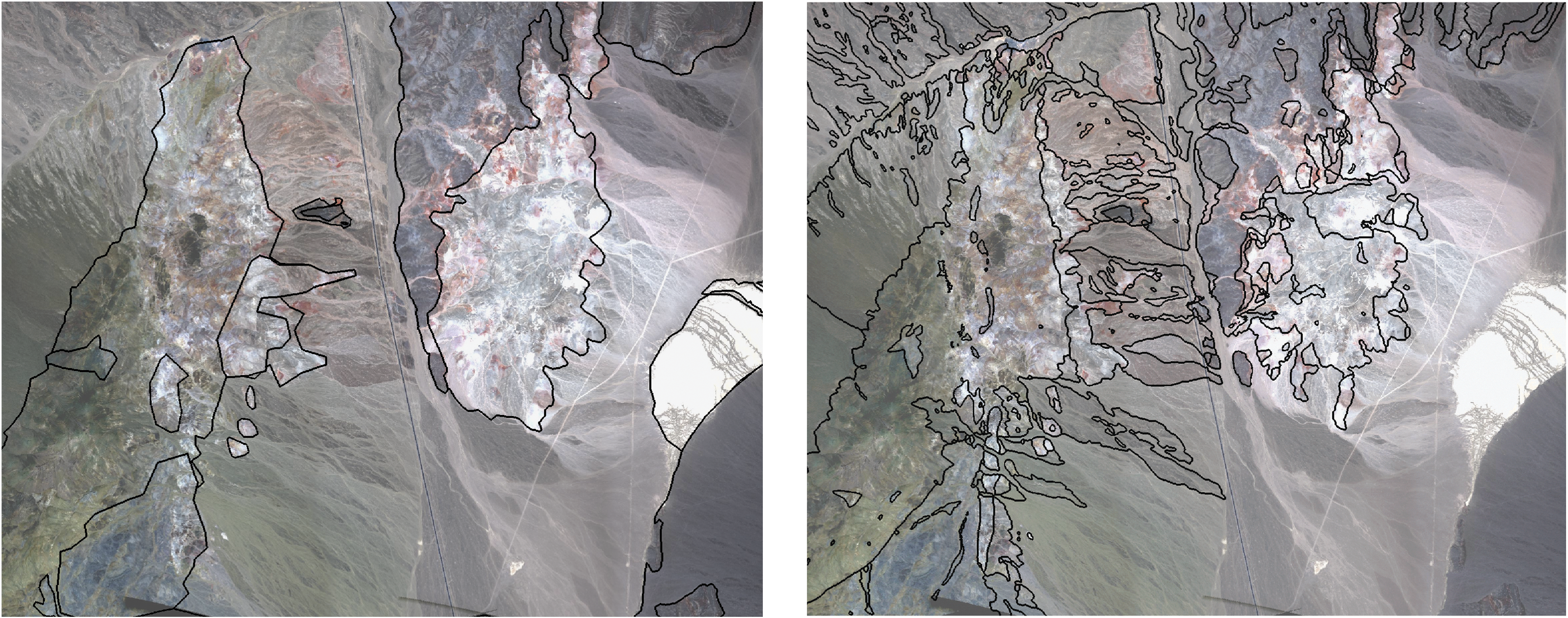
Our partitioned model uses spatial labelings of the scene created by geologic experts. These partitions are based on expert domain knowledge about the location of likely unit boundaries. Each unit could have a different geologic classification, and they are treated independently. Figure 2 shows some possible partitionings of Cuprite. The left panel uses geologic units delineated by a geologist analyzing high-resolution visible wavelength satellite data. The regions are taken to have different surface compositions based on visual cues, though their proper classifications are initially unknown. The right panel shows units described by Albers and Stewart (1972) and Ashley and Abrams (1980) and modified in Swayze et al. (2014). These unit boundaries and classifications are an expert assessment of extensive ground truth campaigns, in situ fieldwork, rich isotopic measurements, dating, and remote spectroscopy. The true classification of these units into their geologic origin and alteration states is withheld during the simulation and used as ground truth for comparing measurement strategies. We also rely on alteration maps reproduced in Figs. 4 and 17(A) of (Swayze et al., 2014), which show the locations of the different Cuprite alteration zones.

FIG. 2.

Left: Photogeologic unit boundaries drawn by hand using high spatial resolution visible wavelength data. Right: Alteration unit boundaries drawn by hand during detailed geologic surveys, courtesy of Albers and Stewart (1972), Ashley and Abrams (1980), and Swayze et al. (2014).

FIG. 4.

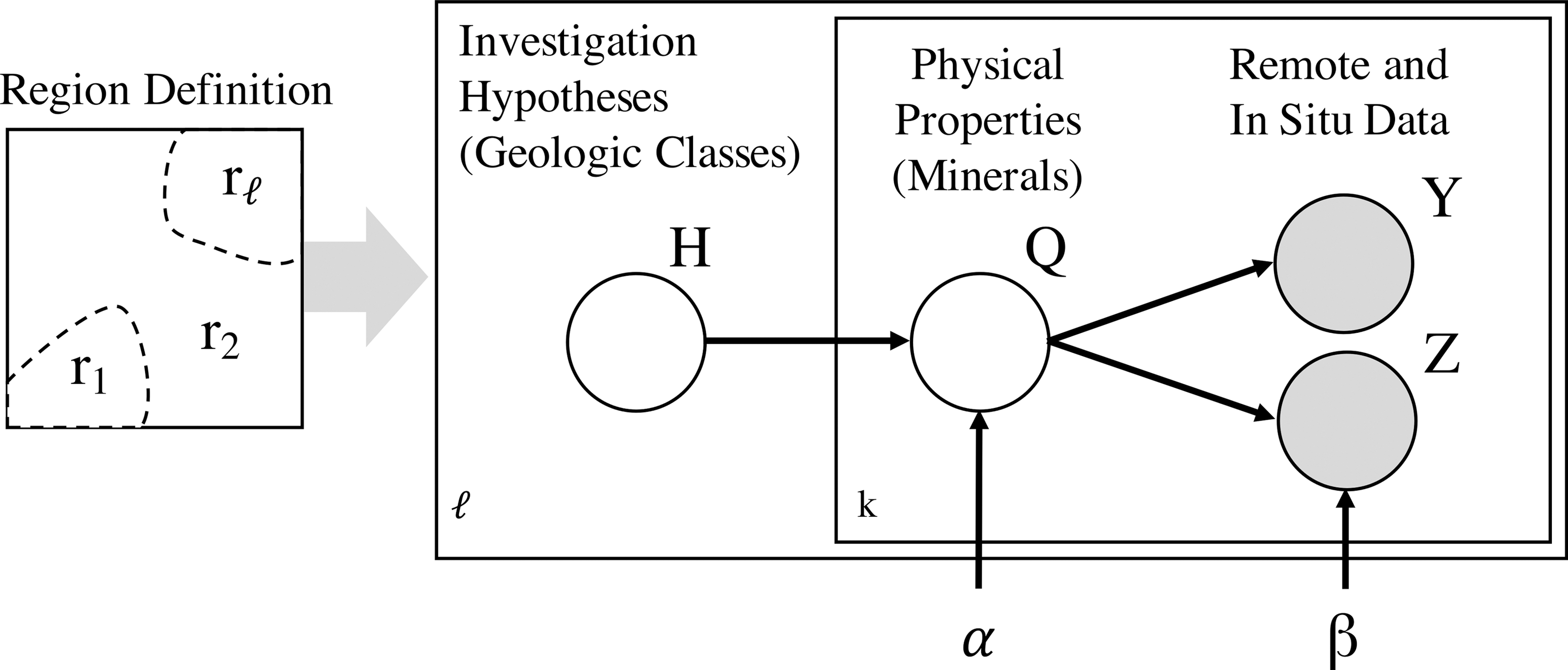
Graphical representation of random variables in the model.

Our remote sensing alternative begins with multiband remote data over the entire site acquired by ASTER (Rowan et al., 2003). The ASTER data can delineate major geologic unit boundaries, but it cannot recognize unique minerals due to the limited number and coarse resolution of instrument channels. ASTER's visible/shortwave infrared channels have center wavelengths at 560, 660, 820, 1650, 2165, 2205, 2260, 2330, and 2395 nm and provide spatial resolutions of 15 m in visible wavelengths and 30 m in the shortwave infrared. The ASTER data is atmospherically corrected with the additional cross-talk correction described in Iwasaki and Tonooka (2005). We discretize ASTER observations into a small number (n = 1000) of categorical labels. We then apply principal component analysis (PCA) that reduces the nine VSWIR channels to five, capturing 99.9% of total variance (Fig. 3), and discretize these observations into categorical observations with k-means clustering. The clustering input space consists of the five PCA coefficients, and the latitude and longitude position of the pixel, scaled to even the influence of spatial and spectral components. The spatial component limits the geographic extent of ASTER surface categories, permitting similar ASTER values from separated locations to have different interpretations. This is important because the ASTER spectra taken alone are ambiguous. The total dimensionality of Cuprite is significantly higher than the five dimensions resolved by ASTER. ASTER shows local differences such as delineations of major surface units, but its measurements do not uniquely determine geologic origins.

FIG. 3.

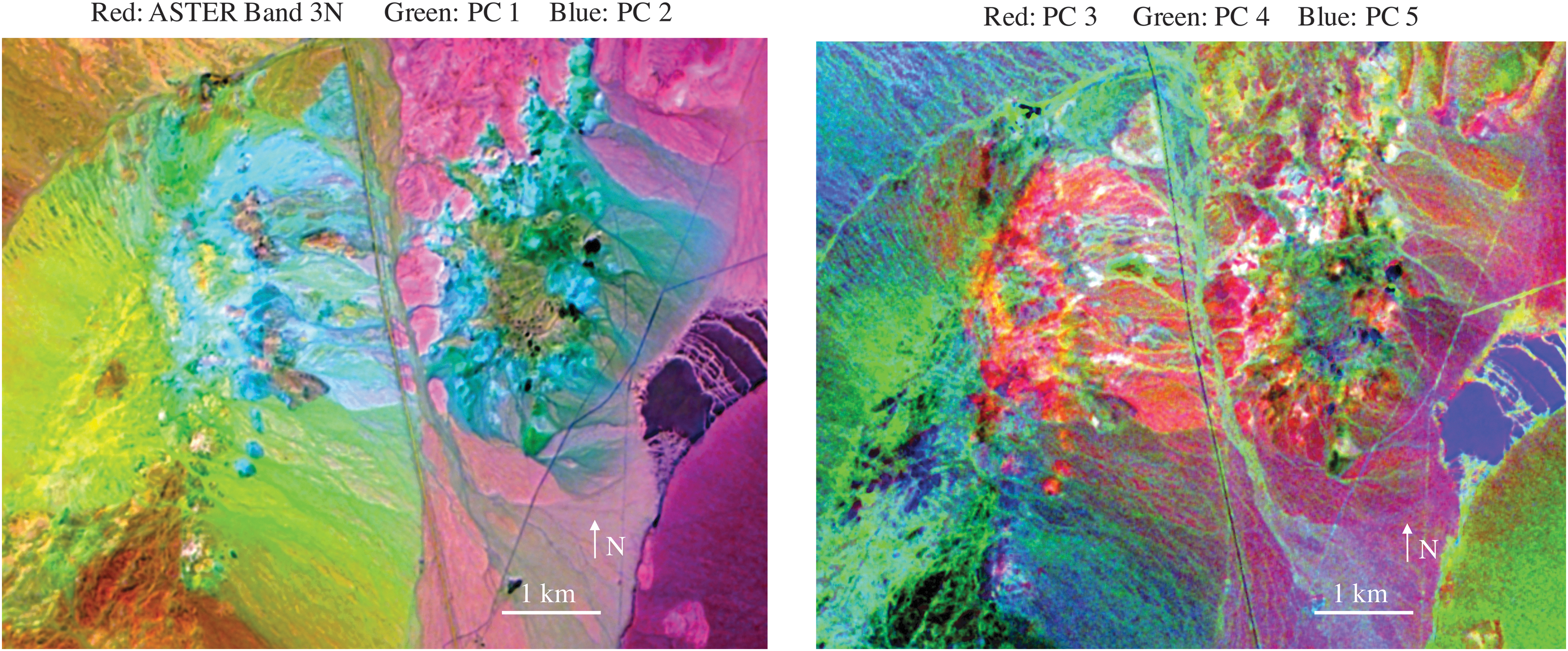
Left: RGB composite. Red is ASTER channel 3N intensity; green and blue are the 2 first principal components of ASTER channels. Right: RGB composite assigning ASTER principal components 3, 4, and 5 to red, green, and blue, respectively.

For the experiments that follow, we posit a remote rover platform with a VSWIR spectrometer. As the in situ explorer observes minerals within a geologic unit, these measurements gradually provide information about the unit origin and alteration history. We simulate in situ spectroscopy using spectra from high-spatial-resolution data cubes acquired by AVIRIS-NG (Green et al., 1998; Hamlin et al., 2011; Thompson et al., 2018). AVIRIS-NG mapped the area during overflights in June 2014 with a ground sampling distance of 3.9 m per pixel, measuring spectral radiance from 380 to 2510 nm at approximately 5 nm sampling. We first calibrate the AVIRIS-NG data using methods of Thompson et al. (2018), then project the radiance spectra to a georectified grid using a camera model, a local Digital Elevation Model, and the onboard inertial measurement and global positioning system data from the instrument. Finally, we atmospherically correct the result using the approach of Thompson et al. (2015b) with the aerosol estimation of Thompson et al. (2017). We use a reference spectrum from a spectrally smooth surface, a dry lakebed known as Stonewall Playa, as a smooth reference. This defines multiplicative smoothing coefficients to correct residual errors in the final reflectance data. Such errors are generally caused by minor inaccuracies in the atmospheric radiative transfer model (Thompson et al., 2015b), and a single correction vector can correct the entire scene. We validate radiometric calibration and atmospheric correction in combination, by comparing remote measurements to GPS-tagged hand samples collected at the site. We characterized samples in the laboratory with an ASD FieldSpec 3 spectrometer, averaging 100 contact probe measurements to obtain a noise-free signal. Hand-selected samples inevitably differ from the heterogeneous pixels observed by AVIRIS-NG at 4 m spatial sampling, but the reference measurements can validate that similar mineral features appear remotely.

We interpret spectra with the Tetracorder 5 algorithm for material detection, identification, and mapping (Clark et al., 2003, 2010; Clark et al., 2015). Tetracorder 5 includes an expanded expert system with additional minerals, organics, and other materials, and more advanced algorithms for analysis including shoulderness and curved continua. Its core is least-squares fitting of continuum-removed absorption features and an extensive library of mineral types found at Cuprite. The result is a matrix of detections indicating the presence of different minerals at every pixel of the high-resolution AVIRIS-NG scene. We combine this data set into a mosaic (Fig. 1) and assign a unique reflectance spectrum to every location. We then use ground control points to coregister this map with the ASTER data. Residual reprojection errors of approximately 10 m are within the size of the ASTER pixels. Our experiments simulate in situ data by drawing subsets from the spectroscopic data set, selecting locations to emulate different rover traverses and data collection strategies, and the resulting impact on interpretations of remote data.

2.3. Probabilistic model

To quantify the information gain of new measurements, we refine the STM into a probabilistic model with the investigation objectives as unknown random variables. The model relates the alternative geologic classifications to the appearance of different minerals, which in turn determines the probability of specific instrument measurements. A common information metric is the Shannon entropy describing the number of bits of uncertainty (Cover and Thomas, 2006). Beneficial measurements increase confidence in geologic classifications, reducing the entropy of the objective variables (Lindley, 1956; Bernardo, 1979; Paninski, 2005). Bayesian experimental design (Chaloner and Verdinelli, 1995) can then optimize future measurement plans and provide the best expected reduction in uncertainty. This could assist mission planning but also enables more adaptive robotic autonomy. With each communication event, mission planners can transmit the variables of interest and the probabilistic models relating them to instrument data. Then the robot can adapt measurement plans in real time to reflect incoming data and opportunistic scientific discoveries.

In service of a controlled experiment, we use the simplest possible model that preserves generality. For the partitioned model, we split the explored environment into disjoint units, each encompassing many potential measurement locations (Fig. 4), and carry a distinct independent objective hypothesis variable about the origin for each unit. For the remote sensing model, the AVIRIS-NG pixel locations are all separate “units,” but neighboring locations are often implicitly associated by having similar remote measurements. In both cases, the pixels of the AVIRIS-NG image cube are the measurable locations with high-resolution AVIRIS-NG data standing in as a simulation of the in situ spectra that would be obtained. For simplicity, we define all probabilities over categorical values, permitting inference by brute force summation of conditional probability tables.

Figure 4 shows the key components of the probabilistic model:

• The map contains \documentclass{aastex}\usepackage{amsbsy}\usepackage{amsfonts}\usepackage{amssymb}\usepackage{bm}\usepackage{mathrsfs}\usepackage{pifont}\usepackage{stmaryrd}\usepackage{textcomp}\usepackage{portland, xspace}\usepackage{amsmath, amsxtra}\usepackage{upgreek}\pagestyle{empty}\DeclareMathSizes{10}{9}{7}{6}\begin{document}$$\ell$$ \end{document} independent, disjoint unit regions \documentclass{aastex}\usepackage{amsbsy}\usepackage{amsfonts}\usepackage{amssymb}\usepackage{bm}\usepackage{mathrsfs}\usepackage{pifont}\usepackage{stmaryrd}\usepackage{textcomp}\usepackage{portland, xspace}\usepackage{amsmath, amsxtra}\usepackage{upgreek}\pagestyle{empty}\DeclareMathSizes{10}{9}{7}{6}\begin{document}$$R = \{ {r_1} , \ldots , {r_ \ell } \} $$ \end{document} .

• Both Objective I (broad geologic categories) and Objective II (alteration state) aim to assign classifications for each region. We can represent either goal by treating regions' classes as variables, written h_i , that together comprise the set \documentclass{aastex}\usepackage{amsbsy}\usepackage{amsfonts}\usepackage{amssymb}\usepackage{bm}\usepackage{mathrsfs}\usepackage{pifont}\usepackage{stmaryrd}\usepackage{textcomp}\usepackage{portland, xspace}\usepackage{amsmath, amsxtra}\usepackage{upgreek}\pagestyle{empty}\DeclareMathSizes{10}{9}{7}{6}\begin{document}$$H = \{ {h_1} , \ldots , {h_ \ell } \} ,$$ \end{document} h_i ∈ H.

• Variables q describe local physical properties at k different observation locations for a particular region. Together they form the region's set \documentclass{aastex}\usepackage{amsbsy}\usepackage{amsfonts}\usepackage{amssymb}\usepackage{bm}\usepackage{mathrsfs}\usepackage{pifont}\usepackage{stmaryrd}\usepackage{textcomp}\usepackage{portland, xspace}\usepackage{amsmath, amsxtra}\usepackage{upgreek}\pagestyle{empty}\DeclareMathSizes{10}{9}{7}{6}\begin{document}$$Q = \{ {q_1} , \ldots , {q_k} \} $$ \end{document} , q_i ∈ Q. These indicate the presence of specific minerals within the unit. A hyperparameter α governs the strength of association between the minerals and geologic classes.

• In situ measurements are random variables \documentclass{aastex}\usepackage{amsbsy}\usepackage{amsfonts}\usepackage{amssymb}\usepackage{bm}\usepackage{mathrsfs}\usepackage{pifont}\usepackage{stmaryrd}\usepackage{textcomp}\usepackage{portland, xspace}\usepackage{amsmath, amsxtra}\usepackage{upgreek}\pagestyle{empty}\DeclareMathSizes{10}{9}{7}{6}\begin{document}$$Y = \{ {y_1} , \ldots , {y_k} \} $$ \end{document} . We assume that each in situ spectrum is unambiguous and uniquely identifies the mineral at that location. For any region, the number of independent locations is k.

• Prior remote sensing data at each location is a random variable \documentclass{aastex}\usepackage{amsbsy}\usepackage{amsfonts}\usepackage{amssymb}\usepackage{bm}\usepackage{mathrsfs}\usepackage{pifont}\usepackage{stmaryrd}\usepackage{textcomp}\usepackage{portland, xspace}\usepackage{amsmath, amsxtra}\usepackage{upgreek}\pagestyle{empty}\DeclareMathSizes{10}{9}{7}{6}\begin{document}$$Z = \{ {z_1} , \ldots , {z_k} \} $$ \end{document} , z_i ∈ Z. For convenience, each remote cluster is also associated with a single unique (but unknown) mineral. A vector β of free parameters controls the strength of these relationships.

This model does not restrict the domains of any variables. We posit a hierarchical dependence structure in which H and {Y, Z} are independent given Q (Fig. 4). Using the chain rule, the joint probability model of H, Q, Y, and Z is \documentclass{aastex}\usepackage{amsbsy}\usepackage{amsfonts}\usepackage{amssymb}\usepackage{bm}\usepackage{mathrsfs}\usepackage{pifont}\usepackage{stmaryrd}\usepackage{textcomp}\usepackage{portland, xspace}\usepackage{amsmath, amsxtra}\usepackage{upgreek}\pagestyle{empty}\DeclareMathSizes{10}{9}{7}{6}\begin{document} \begin{align*} P \left( {H , { \rm{ }}Q , { \rm{ }}Y , { \rm{ }}Z} \right) { \rm{ }} = P \left( H \right) P \left( {Q \vert H} \right) P \left( {Y \vert Q} \right) P \left( {Z \vert Q} \right) \tag{1} \end{align*} \end{document}

The term P(H) represents the prior distribution over geologic classifications, capturing domain knowledge, prior expectations about the site, or previous rounds of exploration. P(Q|H) captures the strength of association between geologic classes and mineral features observable at the surface. This is a stochastic relationship because mineral appearances do not exactly determine the geologic origin. Even after many minerals are observed from a site, there may still be uncertainty in the geologic class. P(Y|Q) and P(Z|Q) respectively give the in situ and remote mineral measurement processes, incorporating physical noise as well as any algorithmic classification error or ambiguity. In this case study the spectroscopic data provided by AVIRIS-NG perfectly describes the mineral Q so P(Y|Q) is a Boolean matrix. In contrast, the remote ASTER data is ambiguous so P(Z|Q) is stochastic. Integrating over variables yields \documentclass{aastex}\usepackage{amsbsy}\usepackage{amsfonts}\usepackage{amssymb}\usepackage{bm}\usepackage{mathrsfs}\usepackage{pifont}\usepackage{stmaryrd}\usepackage{textcomp}\usepackage{portland, xspace}\usepackage{amsmath, amsxtra}\usepackage{upgreek}\pagestyle{empty}\DeclareMathSizes{10}{9}{7}{6}\begin{document} \begin{align*} P ( H , Y , Z ) = P ( H ) \mathop \sum \limits_Q \; {P ( Q \vert H ) P ( Y \vert Q ) P ( Z \vert Q ) } \tag{2} \end{align*} \end{document} \documentclass{aastex}\usepackage{amsbsy}\usepackage{amsfonts}\usepackage{amssymb}\usepackage{bm}\usepackage{mathrsfs}\usepackage{pifont}\usepackage{stmaryrd}\usepackage{textcomp}\usepackage{portland, xspace}\usepackage{amsmath, amsxtra}\usepackage{upgreek}\pagestyle{empty}\DeclareMathSizes{10}{9}{7}{6}\begin{document} \begin{align*} P ( Y , Z ) = \mathop \sum \limits_H { \;P ( H ) \; \mathop \sum \limits_Q { \;P ( Q \vert H ) P ( Y \vert Q ) P ( Z \vert Q ) } } \tag{3} \end{align*} \end{document}

From the definition of conditional probability, we have \documentclass{aastex}\usepackage{amsbsy}\usepackage{amsfonts}\usepackage{amssymb}\usepackage{bm}\usepackage{mathrsfs}\usepackage{pifont}\usepackage{stmaryrd}\usepackage{textcomp}\usepackage{portland, xspace}\usepackage{amsmath, amsxtra}\usepackage{upgreek}\pagestyle{empty}\DeclareMathSizes{10}{9}{7}{6}\begin{document} \begin{align*} P \left( { Y , Z \vert H } \right) { \rm { } } = { \frac { P ( Y , Z , H ) } { P ( H ) } } \tag { 4 } \end{align*} \end{document}

Consequently, the conditional probability of a hypothesis given a remote measurement is \documentclass{aastex}\usepackage{amsbsy}\usepackage{amsfonts}\usepackage{amssymb}\usepackage{bm}\usepackage{mathrsfs}\usepackage{pifont}\usepackage{stmaryrd}\usepackage{textcomp}\usepackage{portland, xspace}\usepackage{amsmath, amsxtra}\usepackage{upgreek}\pagestyle{empty}\DeclareMathSizes{10}{9}{7}{6}\begin{document} \begin{align*} P \left( { H \vert Z } \right) = { \frac { P ( Z \vert \;H ) P ( H ) } { P ( Z ) } } \tag { 5 } \end{align*} \end{document}

And the conditional probability of a hypothesis given an in situ measurement is \documentclass{aastex}\usepackage{amsbsy}\usepackage{amsfonts}\usepackage{amssymb}\usepackage{bm}\usepackage{mathrsfs}\usepackage{pifont}\usepackage{stmaryrd}\usepackage{textcomp}\usepackage{portland, xspace}\usepackage{amsmath, amsxtra}\usepackage{upgreek}\pagestyle{empty}\DeclareMathSizes{10}{9}{7}{6}\begin{document} \begin{align*} P \left( { H \vert Z , Y } \right) = { \frac { P ( Y , \;Z \vert \;H ) P ( H ) } { P ( Y , \;Z ) } } \tag { 6 } \end{align*} \end{document}

Note that this is equivalent to performing Bayesian inference, with P(H) the initial belief and P(H|Y, Z) the posterior probability.

2.4. Quantification of mineral/unit associations

We use multiple methods to estimate conditional probability relationships. We first set the relationship between minerals and geologic classes, P(Q|H). Many minerals may be consistent with one class. We begin by simply eliciting these consistency assessments from a geologist, and we write them as a matrix with one row for each geologic class and one column for each possible mineral. One can interpret this consistency matrix as a conditional probability table P(Q|H) with each row (geologic class) a categorical distribution. In theory, a binary matrix is inappropriate with real measurement noise and inevitable spilling of minerals across adjacent units. However, it is far easier for geologists to state relationships of logical consistency than to assign quantitative probabilities. Consequently, we first define a binary (Boolean) consistency matrix and then use statistical fits with actual data to soften these hard assessments. Each row is populated by two continuous probabilities: φ(1 − α) when the mineral is consistent with the class, and φα otherwise. Here, α is a free parameter, a small value governing the probability that an inconsistent mineral is observed. It also controls the rate at which multiple mineral observations within a unit improve its classification certainty. The variable φ is a normalizing factor.

The α parameter depends on the characteristics of the site and the geographic footprint of the sensor. We fit α using a set of training data, selecting the value that maximizes the data likelihood. This is challenging because true unit labels are usually not available for remote exploration de novo. Instead, we develop a method to determine α from arbitrary new scenes, exploiting the fact that, in this case study, geologic units are spatially uniform and contiguous—neighboring locations are likely to share the same geologic class. We define neighboring locations by oversegmenting an AVIRIS-NG scene, as in prior imaging spectroscopy research using superpixels (Thompson et al., 2011). Since most of these small regions do not cross geologic class boundaries, any mutually inconsistent minerals within a superpixel are related to the influence of α. To form superpixels, we first reduce the dimensionality of the high-dimensional data set to a small number (typically 5–10) using PCA, which intentionally eliminates most of the spectral diversity while leaving a handful of mutually orthogonal color channels that would capture differentiations between units. We shatter the image into small spectrally homogeneous neighborhoods using the SLIC segmentation algorithm (Achanta et al., 2012). This produces a set of disjoint contiguous regions that are spectrally homogeneous. We only use the PCA-reduced representation during the unit segmentation stage, and retain the full spectrum for spectroscopic mineral detection.

After segmentation, we calculate maximum-likelihood α values using the most probable assignment of the geologic class for each segment S. We write the mineral observations in each segment S as instances q ∈ S and the log likelihood of the entire dataset as \documentclass{aastex}\usepackage{amsbsy}\usepackage{amsfonts}\usepackage{amssymb}\usepackage{bm}\usepackage{mathrsfs}\usepackage{pifont}\usepackage{stmaryrd}\usepackage{textcomp}\usepackage{portland, xspace}\usepackage{amsmath, amsxtra}\usepackage{upgreek}\pagestyle{empty}\DeclareMathSizes{10}{9}{7}{6}\begin{document} \begin{align*}{{\rm L}_ \alpha } = \mathop \sum \limits_S {{{ \inf }_c}} \; \mathop \sum \limits_{q \in S} { \log } \left[ {{{\bf 1}_{q , c}} \phi ( 1 - \alpha ) + ( 1 - {{\bf 1}_{q , c}} ) \phi ( \alpha ) } \right] \tag{7} \end{align*} \end{document}

where c represents the geologic class: a possible value for the investigation objective H. Inf_c represents the infinum, the value of c that minimizes the terms at right. The indicator function 1 _q,c evaluates to unity when mineral q is consistent with the most likely geologic class c, and zero otherwise. A simple one-parameter optimization over α finds the best fit, bringing P(H|Q) into agreement with the measurement data.

2.5. Classification with remote sensing data

We take AVIRIS-NG data to be perfectly diagnostic of each mineral, but ASTER observations have some nonzero probability of association with multiple minerals. We set these conditional probabilities by simply counting the appearance of each mineral within each ASTER observation type. We define a conditional probability table of size [number of remote observation possibilities] × [number of minerals], parameterized by a vector β with one element per table entry. The table records the number of observations of each mineral associated with each remote class. We turn these values into probabilities by normalizing along each row. This strategy is unstable when the number of measurements is small or biased, leading to overconfident classifications. To avoid this, we constrain the table with priors, expressed as a table of Dirichlet pseudocounts parameterized by β. Specifically, a row β_j represents the prior probability, in pseudocounts, for the appearance of each mineral within that ASTER label, with a number of elements equal to the number of minerals. We conservatively initialize the table with pseudocounts that imply a uniform distribution of geologic classes, while simultaneously not favoring any one mineral. There are many potential pseudocount assignments that would accomplish this. We solve jointly for all pseudocounts by nonlinear least-squares optimization of the following cost function, where C is the matrix representing conditional probabilities P(Q|H) and n is the number of geologic classes: \documentclass{aastex}\usepackage{amsbsy}\usepackage{amsfonts}\usepackage{amssymb}\usepackage{bm}\usepackage{mathrsfs}\usepackage{pifont}\usepackage{stmaryrd}\usepackage{textcomp}\usepackage{portland, xspace}\usepackage{amsmath, amsxtra}\usepackage{upgreek}\pagestyle{empty}\DeclareMathSizes{10}{9}{7}{6}\begin{document} \begin{align*} f ( { \beta _j} ) = {{ \beta \prime }_j}{ \bf {C}} - 1 / n{ \vert _2} + \gamma \vert { \beta _j} - 0.5{ \vert _2} \tag{8} \end{align*} \end{document}

The symbol β′_j is the pseudocount vector normalized to represent probabilities. Pipe notation |.|₂ represents L2 normalization. The second additive cost is a penalty promoting similarity to a Jeffrys prior, an uninformed prior over mineral observations. A small regularization coefficient γ balances this tendency against uniform geologic classifications. The end result is a fully defined initial probability model, with pseudocounts that are very similar to an uninformed Jeffrys prior and that imply a uniform distribution of geologic classes.

2.6. Entropy and information gain

The completed model defines different measurement plans' information value relative to their costs. Given any preexisting remote data Z, we quantify the current state of classification certainty using the Shannon entropy of each region in R as \documentclass{aastex}\usepackage{amsbsy}\usepackage{amsfonts}\usepackage{amssymb}\usepackage{bm}\usepackage{mathrsfs}\usepackage{pifont}\usepackage{stmaryrd}\usepackage{textcomp}\usepackage{portland, xspace}\usepackage{amsmath, amsxtra}\usepackage{upgreek}\pagestyle{empty}\DeclareMathSizes{10}{9}{7}{6}\begin{document} \begin{align*} I ( H \vert Z ) = \mathop \sum \limits_{i = 1}^ \ell { \mathop \sum \limits_c { - P ( {h_i} = c \vert Z ) \log \;P ( {h_i} = c \vert Z ) } } \tag{9} \end{align*} \end{document}

This quantity measures the uncertainty of H. After an in situ observation y_j , the resulting posterior entropy is \documentclass{aastex}\usepackage{amsbsy}\usepackage{amsfonts}\usepackage{amssymb}\usepackage{bm}\usepackage{mathrsfs}\usepackage{pifont}\usepackage{stmaryrd}\usepackage{textcomp}\usepackage{portland, xspace}\usepackage{amsmath, amsxtra}\usepackage{upgreek}\pagestyle{empty}\DeclareMathSizes{10}{9}{7}{6}\begin{document} \begin{align*} I ( H \vert {y_j} , \;Z ) = \mathop \sum \limits_{i = 1}^ \ell { \mathop \sum \limits_c { - P ( {h_i} = c \vert {y_j} , \;Z ) \log \;P ( {h_i} = c \vert {y_j} , \;Z ) } } \tag{10} \end{align*} \end{document}

Reductions in posterior entropy can quantify the improvement in uncertainty expected, or achieved, with different sampling strategies, making the quantity important for experimental design. In particular, the expected information gain is a popular objective function for information-driven action selection (Lindley, 1956; Bernardo, 1979; Chaloner and Verdinelli, 1995; Paninski, 2005). It is defined as the expected reduction in Shannon entropy after making a future observation (Cover and Thomas, 2006). Before observations are acquired, the expected information gain given n of a set of in situ measurements is \documentclass{aastex}\usepackage{amsbsy}\usepackage{amsfonts}\usepackage{amssymb}\usepackage{bm}\usepackage{mathrsfs}\usepackage{pifont}\usepackage{stmaryrd}\usepackage{textcomp}\usepackage{portland, xspace}\usepackage{amsmath, amsxtra}\usepackage{upgreek}\pagestyle{empty}\DeclareMathSizes{10}{9}{7}{6}\begin{document} \begin{align*} IG \left( {H \vert Y , { \rm{ }}Z} \right) { \rm{ }} = I \left( {H \vert Z} \right) { \rm{ }} - {\rm{E}_P}_{ \left( {Y \vert Z} \right) } \left[ {I \left( {H \vert Y , { \rm{ }}Z} \right) } \right] \tag{11} \end{align*} \end{document}

During each cycle, the robotic explorer collects a sequence of n measurements of minerals. The total number of different combinations is the same as with the support of the multinomial distribution, which makes the information gain challenging to calculate since the expectation in Eq. 11 must consider all possible combinations. In prior work, we demonstrated how this could be overcome using Monte Carlo integration (van den Berg et al., 2003), or more efficiently, by fitting generalized logistic function relationships to Monte Carlo results (Candela et al., 2017). Such measures are beyond the scope of this study, which focuses on the empirical performance of different sampling strategies. We define the empirical information gain as the reduction in Shannon entropy actually achieved after making the observation, that is, the observer's actual improvement in certainty with respect to investigation hypotheses. For an observation at time t, leading to a posterior distribution over hypotheses H^t , the empirical information gain over time t − 1 is \documentclass{aastex}\usepackage{amsbsy}\usepackage{amsfonts}\usepackage{amssymb}\usepackage{bm}\usepackage{mathrsfs}\usepackage{pifont}\usepackage{stmaryrd}\usepackage{textcomp}\usepackage{portland, xspace}\usepackage{amsmath, amsxtra}\usepackage{upgreek}\pagestyle{empty}\DeclareMathSizes{10}{9}{7}{6}\begin{document} \begin{align*} I{G_{{ \rm{emp}}}} \left( {{H^t} \vert Y , \;{Z^t}} \right) = I \left( {{H^t} \vert {Z^t}} \right) - I \left( {{H^{t - 1}}} \right) \tag{12} \end{align*} \end{document}

This expression is computationally tractable and permits retrospective comparisons of measurements acquired by different strategies. We emphasize that the general probabilistic model is also useful for calculating the expected information gain, enabling remote explorers to form new plans in response to recent data, based on the information value they expect from those observation sequences. However, from now on, when we refer to information gain, we mean the empirical gain calculated after measurements (Eq. 12 rather than Eq. 11).

Remote sensing is a special case, since each new in situ measurement provides information to interpret ambiguous ASTER data. The model can capture this by treating β as a free variable and reestimating it over time. This simply involves updating β using the counts provided by new measurements, extrapolating from local observations to refine the entire map. If β is random, this update is implicit in the equations above. Sampling planners (Arora et al., 2017; Candela et al., 2017) could exploit this learning on the fly, refitting models during the sampling step resulting in policies that “plan to learn.” This would enable the remote agent to balance (a) information gain provided directly by in situ observations and (b) that which would occur indirectly as a result of better interpretations of remote data.

2.7. Experimental method

Our experiments compare different in situ data collection strategies, evaluating their value with respect to Objectives I and II (Tables 1 and 2). We use the Tetracorder classifications of remote AVIRIS-NG data to represent the in situ measurements. For each site of interest, we simulate a robotic explorer acquiring measurements along a transect and then updating the probabilistic model. Our experiments consider long transects B1 and B2 and the short transects A1–A10. The short transects emulate exploration by a rover during a single command cycle. Sites A1–A8 in Table 3 are locations identified in Swayze et al. (2014) and prior literature as areas of special interest with high spectral purity and/or representativeness of a specific mineral type. Using these representative regions minimizes ambiguity in the spectroscopic measurement, permitting a more controlled test of the spatial models and inference method. We include site A9 as a null case—the Stonewall playa traverse, which lies exclusively on a featureless playa; it is spectrally uniform and is not representative of the site as a whole. There may be some trace chalcedony from alteration in the eastern center, but the playa sediment itself is mostly montmorillonite, and the latter is spectrally dominant. Therefore, we expect A9 to provide less information gain toward Objective II. We also add site A10 to the Swayze et al. list to represent the northeastern region. Many of these transects cross multiple surficial terrain types, providing the opportunity to sample multiple different minerals. Figure 5 shows photography from the field illustrating the sparse vegetation and open nature of the terrain. The clear visibility of surficial minerals from the air means that a high-spatial-resolution airborne perspective is a good proxy for in situ instruments. We form sampling transects for each location by extending a rover path along the east-west direction with a total length of 200 m, a reasonable maximum daily traverse distance of a capable modern planetary rover. We imagine a spectroscopic measurement to be collected at each possible location along the transect, a total of 50 unique spectra for each site.

FIG. 5.

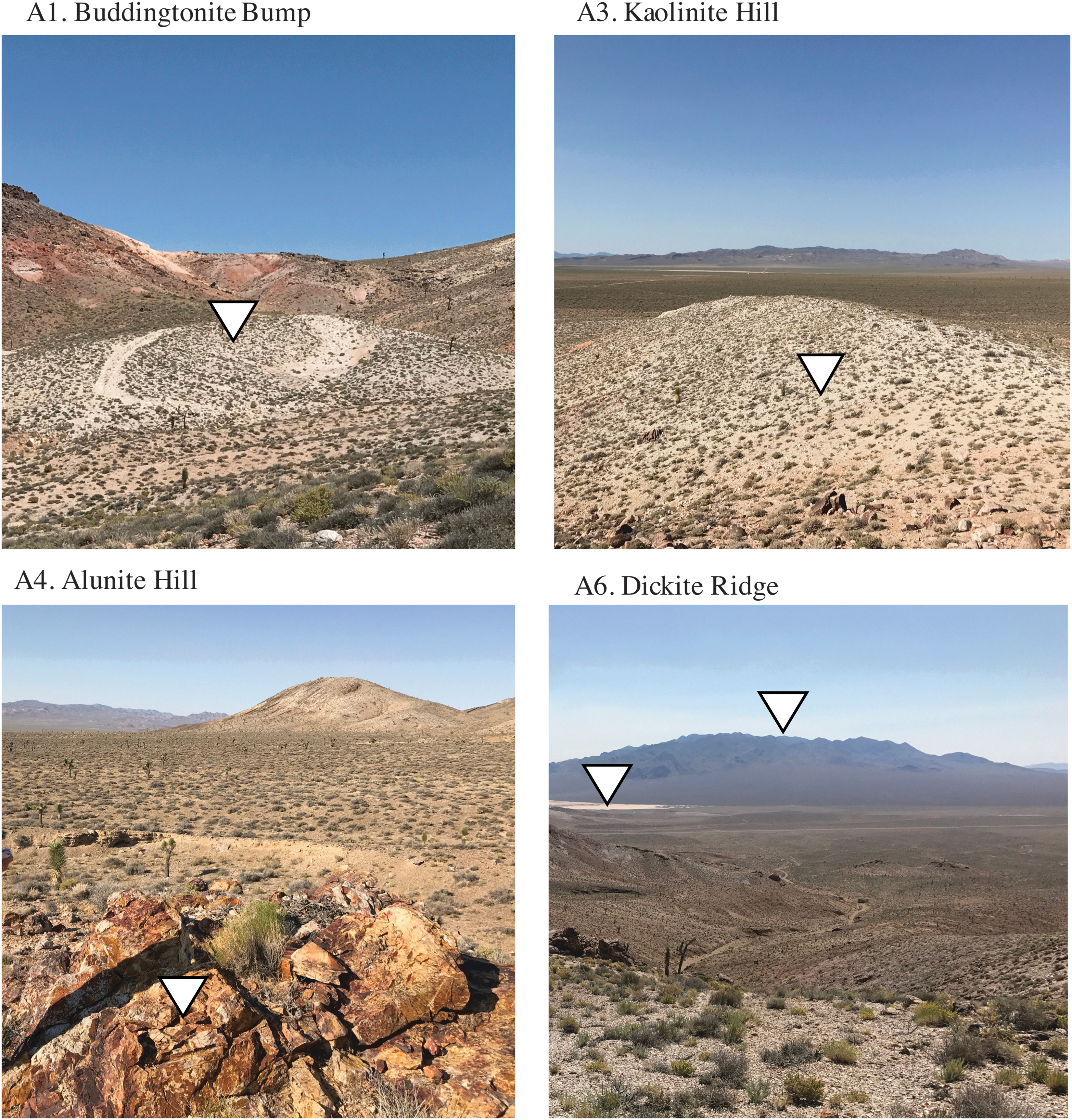
Photography from selected sites. The white triangle icons indicate (A1) a hill composed mainly of the ammonium feldspar buddingtonite, (A3) a hill composed mainly of kaolinite in the eastern center, (A4) jarosite and goethite coatings imparting an orange hue to alunite minerals, and (A6) Stonewall Playa and Stonewall Mountain features, looking southeast from a topographic high point on Dickite Ridge.

Table 3.

Locations of Interest and Transects Illustrated in Figure 1 and Used in Subsequent Simulations

Site	Informal name	North latitude	West longitude	Notes
A1	Buddingtonite Bump	37.54319	117.18677	As in Swayze et al. (2014), Figure 5
A2	Opal Hill	37.54729	117.16713	As in Swayze et al. (2014)
A3	Kaolinite Hill	37.52653	117.17752	As in Swayze et al. (2014), Figure 5
A4	Alunite Hill	37.52400	117.21390	As in Swayze et al. (2014), Figure 5
A5	Quartz/Latite Dike	37.52296	117.22102	As in Swayze et al. (2014)
A6	Dickite Ridge	37.52952	117.22267	As in Swayze et al. (2014)
A7	Pediment Basalt	37.54740	117.20618	As in Swayze et al. (2014)
A8	Opal or Chalcedony	37.53355	117.20961	As in Swayze et al. (2014)
A9	Stonewall Playa	37.53260	117.15823	As in Swayze et al. (2014), Figure 5
A10	Three Minerals	37.55688	117.17583
B1	West Transect	n/a	n/a	As in Swayze et al. (2014)
B2	East Transect	n/a	n/a	As in Swayze et al. (2014)

We also consider a long traverse emulating a multisite rover investigation spanning multiple command cycles. Table 3 locations B1–B2 are the bent linear transect of Swayze et al. (2014), a piecewise linear slice that bisects the eastern and western sides of the site. For both short and long traverses, we evaluate dense sampling that measures every location along the transects, and sparser measurement strategies that acquire data at regular intervals. For each alternative, we perform inference using both prepartitioning and remote sensing representations of spatial correlation. We quantify the benefits of these measurement plans using the posterior Shannon entropy representing uncertainty over geologic classifications (from Eq. 9).

3. Results

3.1. Model parameters

The learned parameters of the probability model reveal the suitability of our conditional probability table representation and the predictive power of the observation data. For example, the best-fitting α values describe the strength of the mineral/class associations. A value of zero would mean that the elicited consistency relationships were never violated. Reassuringly, small α values predominate, meaning the consistency relationships align well with the data. This simultaneously validates the elicited consistency table, the spectroscopic measurements, and the Tetracorder identification. The best α values range from 0.02 to 0.035 depending on the superpixel segment size. Spatial correlations are stronger over smaller distances, smaller areas are more homogeneous, and small segment sizes permit smaller α values. Figure 6 shows the superpixel segmentation for different segment length settings. Larger SLIC segments are more stringent, requiring class homogeneity over wider areas. Figure 7 (left) shows likelihood values for Objective I at each of the superpixel resolutions. For segments of length 320 m, approximately 5% of minerals within segments are mutually inconsistent. For smaller segments of length 40 m, approximately 3% of minerals are mutually inconsistent. Such inconsistencies could be a combination of mixing between units at their peripheries or transport of rock float across unit boundaries. We cannot exclude occasional measurement errors or ambiguity in Tetracorder interpretation of mixed surfaces. Nevertheless, these rates are quite low, indicating that the mineral detections are strongly related to common geologic origins for Objective I. We use the conservative value of α = 0.035 to form conditional probability tables for Objective I.

FIG. 6.

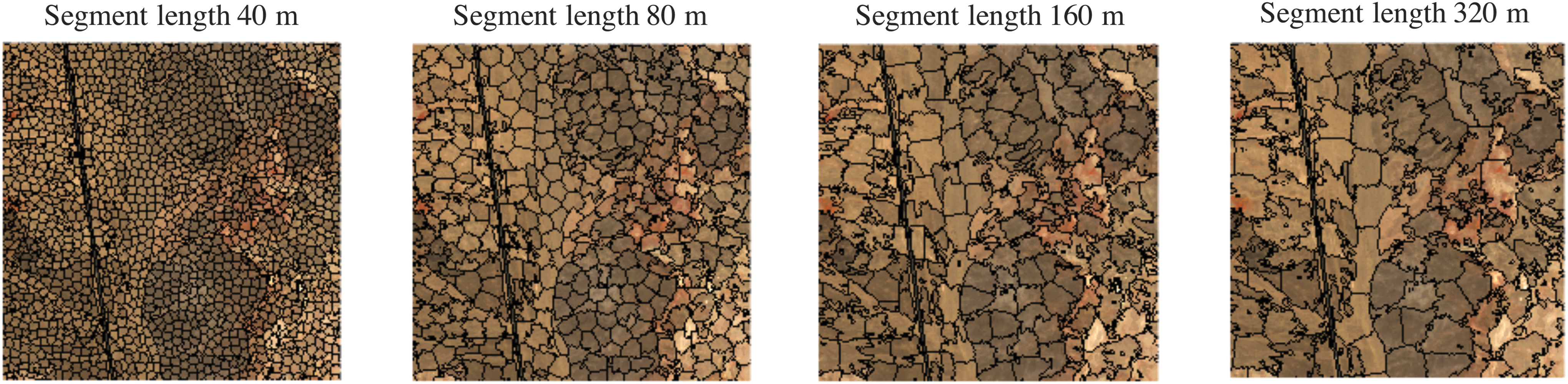
Segmentations using different superpixel window sizes overlaid on a visible-wavelength fragment of the Cuprite scene.

FIG. 7.

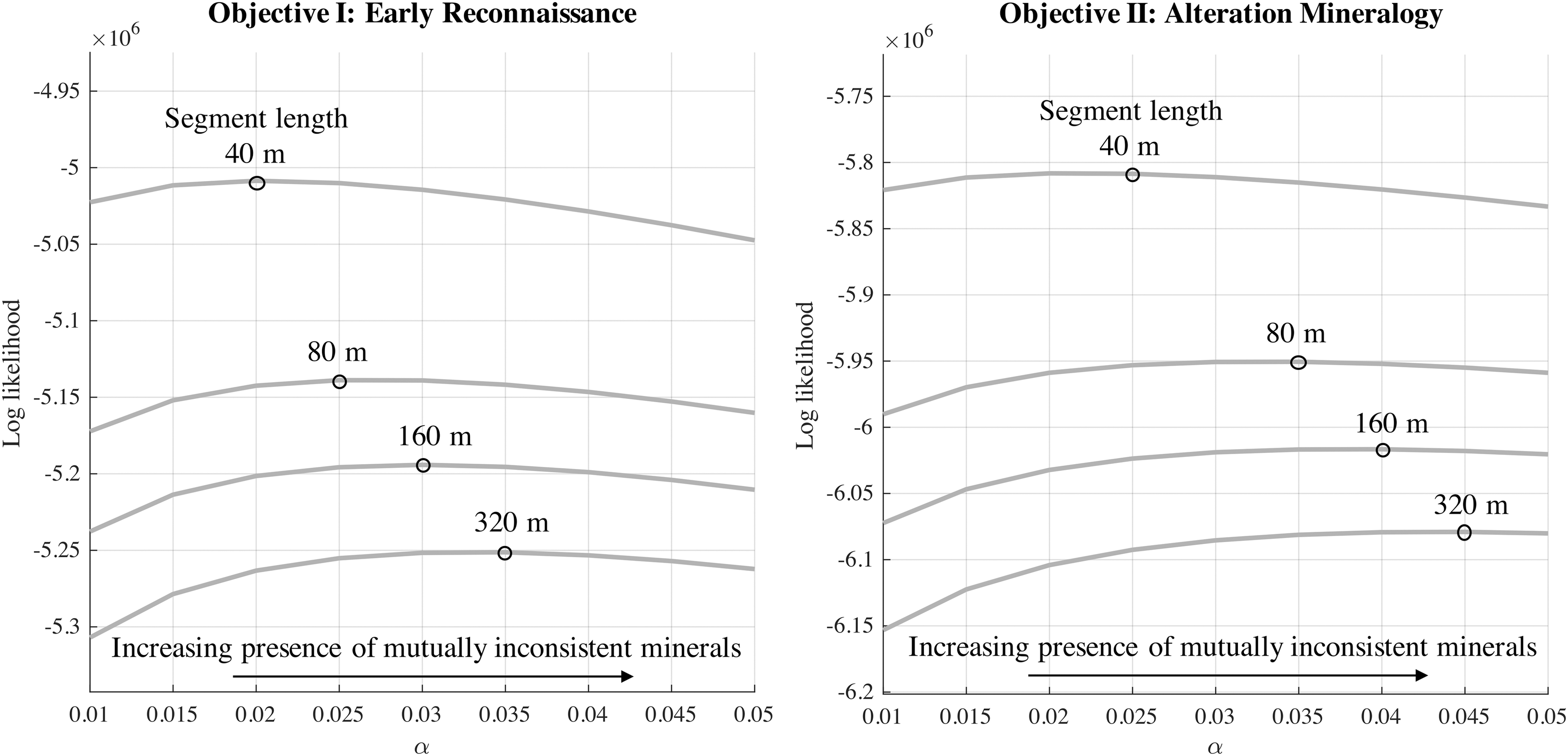
Log likelihood values and best α values at different segmentation resolutions. Left: Optimal α value for Objective I, early reconnaissance. Right: Optimal α values for Objective II, alteration mineralogy.

Refitting α for the more specific investigation (Objective II) produces slightly different results. Figure 7 (right) shows this more refined goal. Here, the best α values are slightly higher, peaking at 0.045 for a superpixel size of 320 m. This is not surprising; Cuprite contains many mixtures of alteration minerals from different classes, both at the peripheries of these zones and in alluvial that source from multiple locations. Figure 7 maps this effect spatially for the 320 m superpixel size, showing the fraction of inconsistent minerals at each superpixel. The fractions are higher for alluvial fans than for outcrop.

3.2. Spectroscopic observations of minerals and geologic class

Contact measurements of field samples align well with the AVIRIS-NG data. Figure 8 shows remote reflectance with that of in situ samples. The remote spectra are the average of a 12 m area from the mosaic. We favor sites A3 (Kaolinite Hill) and A4 (Alunite Hill) for this comparison, because the features are highly distinctive and the compounds of interest are spectrally dominant and more uniformly distributed than at most other locations. Remote and laboratory measurements generally agree to within 1–2% of absolute reflectance, which is surprising given that no continuum removal or continuum-level alignment was performed. The key spectral features from each mineral are present in both data sets, though the AVIRIS-NG data offers higher spectral resolution. This comparison confirms that the reflectance products capture spectral content observable in situ.

FIG. 8.

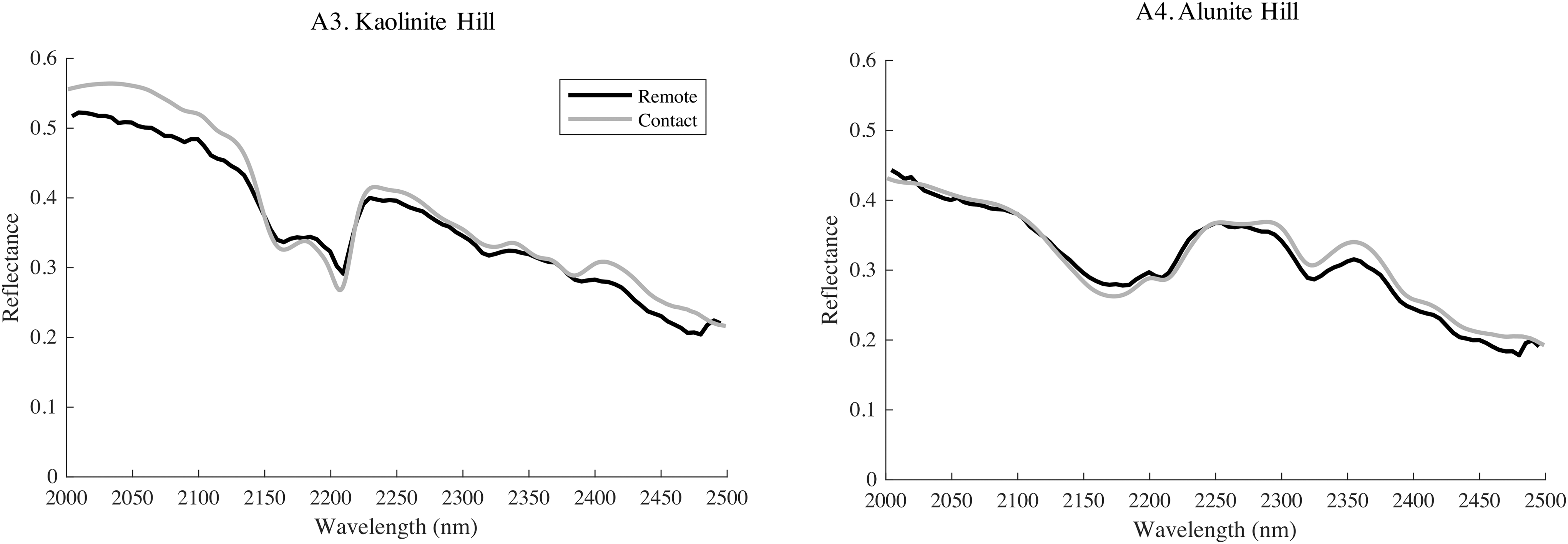
Laboratory contact measurements of samples from each location align well with geolocated AVIRIS-NG spectra from the Cuprite scene.

Next we investigate the remote mineral detections and the geologic classifications they imply for each unit. Initially, we treat each measurement location independently without spatial correlations. At this basic level, the model results are consistent with conventional geologic maps of Cuprite. Table 4 shows the dominant mineral and the most likely classification for each transect with respect to both objectives. Bold classification entries are the most consistent with the mineral map of Swayze et al. (2014). The next columns show classifications for Objective II. The alteration scale represents points along a continuum of possibilities, and we show the two most probable classifications. For Objective I, the model unsurprisingly classifies nearly all the sites as metamorphic/hydrothermal zones, at high probability.

Table 4.

Transect Results

Site	ζ	Dominant spectrum match (n)	Obj. I	Obj. II
A1. Buddingtonite Bump	7	feldspar-buddington.namont2 (16)	MH	AS, A
A2. Opal Hill	5	sioh-hydrated-basaltic-glass (33)	MH	A, K
A3. Kaolinite Hill	7	kaol.75+alun.25 (25)	MH	K, A
A4. Alunite Hill	7	sulfate-alunNa03 (17)	MH	A, K
A5. Quartz/Latite Dike	10	carbonate-calcite (22)	MH	K, WM
A6. Dickite Ridge	9	sulfate+kaolingrp-natroalun+dickite (13)	MH	K, A
A7. Pediment Basalt	8	Kalun+kaol.intmx (11)	MH	K, A
A8. Opal or Chalcedony	9	sioh-chalcedony (17)	MH	HS, A
A9. Stonewall Playa	1	smectite-montmorillonite-na-highswelling (50)	LM, MH	n/a
A10. Three Minerals	10	sioh-hydrated-basaltic-glass (16)	MH	K, A

Columns from left to right indicate the site, the number ζ of distinct minerals detected, the dominant mineral type and its number of appearances in parenthesis, the dominant classifications for Objective I and Objective II. Objective I classifications are MH (Metamorphic/Hydrothermal), I (Igneous), LM (Lacustrine/Marine). Objective II classifications describe alteration zones including AS (Adularia Smectite), A (Alunite), K (Kaolinite), WM (White Mica ± Montmorillonite), and HS (Hydrated Silica). All classifications are consistent with prior literature. Bold entries align with those of (Swayze et al., 2014).

The classification results all align well with conventional interpretations in prior literature. Site A1, Buddingtonite Bump, contains many detections of the mineral buddingtonite, leading to a classification on the alteration scale in the Adularia/Smectite (AS) position. Site A3, Kaolinite Hill, is unsurprisingly dominated by kaolinite, while Site A4, Alunite Hill, shows alunite and Fe sulfate signatures. The sulfate detection agrees with our ground survey that found abundant jarosite at this location (Fig. 5). Site A5, the Quartz/Latite Dike location, was altered after intrusion and is successfully classified by the model as a Metamorphic/Hydrothermal zone. Other phylosillicate minerals lead to a position on the alteration scale near the White Mica ± Montmorillonite category. Site A6, Dickite Ridge, shows spectral matches consistent with dickite, kaolinite, alunite, and sulfates. These are all in agreement with prior results from Swayze et al. (2014). Site A8, labeled Opal or Chalcedony, lies at a border on the Swayze alteration map between alunite and hydrated silica alteration zones. The system corroborates this: a spectrum containing SiOH and Chalcedony is the best match at 17 locations, leading to a hydrated silicate position on the alteration scale. Finally, Site A9 is notable since it does not match cleanly with any hydrothermal alteration minerals. In fact, this uniform playa contains just one spectral signature, a smectite, leading to an ambiguous classification for both objectives. The coarse geologic classification for Objective I is equally consistent with both Lacustrine/Marine and Metamorphic/Hydrothermal zones. It provides no information with respect to the alteration scale, where classification probabilities remain uniform.

3.3. Spatial correlations to infer geologic maps

Next, we incorporate spatial correlations using both partitioning and remote sensing and calculate information gain as well as the posterior unit classifications. Table 5 shows the empirical reduction in entropy of geologic classifications H resulting from each transect. Higher numbers indicate a larger empirical information gain. For the remote sensing case, we show the mean information gain per location in the map. Crossing multiple regions can influence the posterior classification of large areas. For the remote sensing strategy, we show the average information gain per pixel in the resulting map. Due to the spatial clustering used to produce the ASTER labels, each traverse affects only the local area near its spectra, so the overall information gain across the Cuprite scene is relatively low. However, this permits a meaningful comparison between traverses using remote sensing data. The final two columns show the information gain from the prepartitioning strategy. Here, we calculate the total information gain counting each unit's classification as a separate random variable. This results in elevated information gain for traverses like B1 and B2 that cross multiple predefined units.

Table 5.

Transect Results

		Remote sensing		Predefined regions
ID	Site	Obj. I	Obj. II	Obj. I	Obj. II
A1	Buddingtonite Bump	0.001112	0.000130	1.609438	2.377291
A2	Opal Hill	0.001543	0.000003	3.911741	1.097388
A3	Kaolinite Hill	0.002006	0.000178	4.581315	1.791759
A4	Alunite Hill	0.002064	0.000346	3.218876	4.774528
A5	Quartz/Latite Dike	0.001265	0.000087	4.533764	2.466650
A6	Dickite Ridge	0.000678	0.000093	1.609438	2.890371
A7	Pediment Basalt	0.000430	0.000025	2.302584	2.811499
A8	Opal or Chalcedony	0.001267	0.000088	4.605170	3.538221
A9	Stonewall Playa	0.005555	−0.000002	1.203973	0.000000
A10	Three Minerals	0.001537	0.000033	4.605158	2.734835
B1	Eastern Traverse	0.001899	0.000095	4.581315	5.736077
B2	Western Traverse	0.001404	0.000048	4.581315	5.875901

Columns from left to right indicate the transect ID; the informal name of the site or transect; the empirical bits of information gain per map location with respect to Objectives I and II, for a model incorporating remote sensing data; and the empirical bits of information gain per map location for models using predefined homogeneous regions.

Information gains for Objective I are mostly uniform, differing at most by factors of 2–3. This reflects the fact that nearly all traverses contain very compelling evidence for a metamorphic or hydrothermal origin. In other words, nearly any spectra within the Cuprite region will quickly indicate this option as the most likely classification. It is likely that a rover would find it immediately upon arrival at one of sites A1–A8. The exception is site A9, which still provides information toward Objective I due to the fact that it contains very consistent spectra. Information gains for Objective II are generally smaller by an order of magnitude when using the broadband ASTER-class remote sensing. This objective is much subtler than Objective I, and many minerals are consistent with multiple alteration zones. Consequently, splitting traverses across multiple ASTER observation labels dilutes the effects of the most discriminative minerals. The longer transects (B1 and B2) have higher values due to the number of measurements collected and their intersection with many units. The most information-rich short traverses are those crossing large quantities of pure alteration minerals, such as those at the Alunite Hill and Kaolinite Hill transects. This is not surprising, because the high concentration of easily measurable alteration materials provides strong diagnostic information toward both objectives. The Stonewall Playa transect is the least informative. It is completely uniform and contains no spectrally detectable alteration minerals, so it is not actually relevant to Objective II. Indeed, we find this transect provides no significant information gain toward those variables.

These information gains have spatial extent, since they represent improvements in the interpretation of the unit partitions (for the partitioned model) and ASTER observations (for the remote sensing model). Figure 9 shows the posterior entropy improvement per pixel for traverse A1, calculated with respect to the first objective of general coarse geologic classification. This traverse, the “Buddingtonite Bump Transect,” significantly reduces the entropy of terrain units that it crosses. The model learns to interpret the ASTER data, producing an information benefit for areas outside the literal path of the traverse. Improvements in posterior certainty range from over 0.1 bits per pixel to near 0, depending on the consistency of the minerals and the number of distinct spectra associated with each ASTER label. The central area of the transect crosses a uniform Buddingtonite feature and produces the most significant improvement. The right panel shows the relative change in classifications, with red, green, and blue colors corresponding to the Ternary plot at lower right. Green indicates areas of the image that, after the traverse, become more consistent with a hydrothermally altered zone. Indeed, acquiring any in situ data soon results in a higher probability for hydrothermal/metamorphic origins throughout the entire area, consistent with the true geologic interpretation of the site. Figures 10 and 11 show similar patterns for site A3, Kaolinite Hill, and Site A4, Alunite Hill, respectively, which also contain abundant alteration minerals. In contrast, Fig. 12 shows traverse A9, Stonewall Playa, crossing an area that is entirely uniform and devoid of alteration minerals. Here the classification map indicates less consistency with alteration zones. After assimilating the observations, the model indicates that the playa has a different geologic classification altogether, in agreement with the geologists' interpretation of the site. The information gain is still relatively high, indicating that the spectra acquired along this transect are not yet redundant; acquiring a large number of spectra is useful for overcoming the intrinsic ambiguity of the remote sensing data.

FIG. 9.

Left: improvement in posterior entropy (bits per location) calculated for traverse A1 across Buddingtonite Bump. Right: Change in posterior classification probabilities for three of the Objective I geologic classes.

FIG. 10.

Left: Improvement in posterior entropy (bits per location) calculated for traverse A3 across Kaolinite Hill. Right: Change in posterior classification probabilities for three of the Objective I geologic classes.

FIG. 11.

Left: Improvement in posterior entropy (bits per location) calculated for traverse A4 across Alunite Hill. Right: Change in posterior classification probabilities for three of the Objective I geologic classes.

FIG. 12.

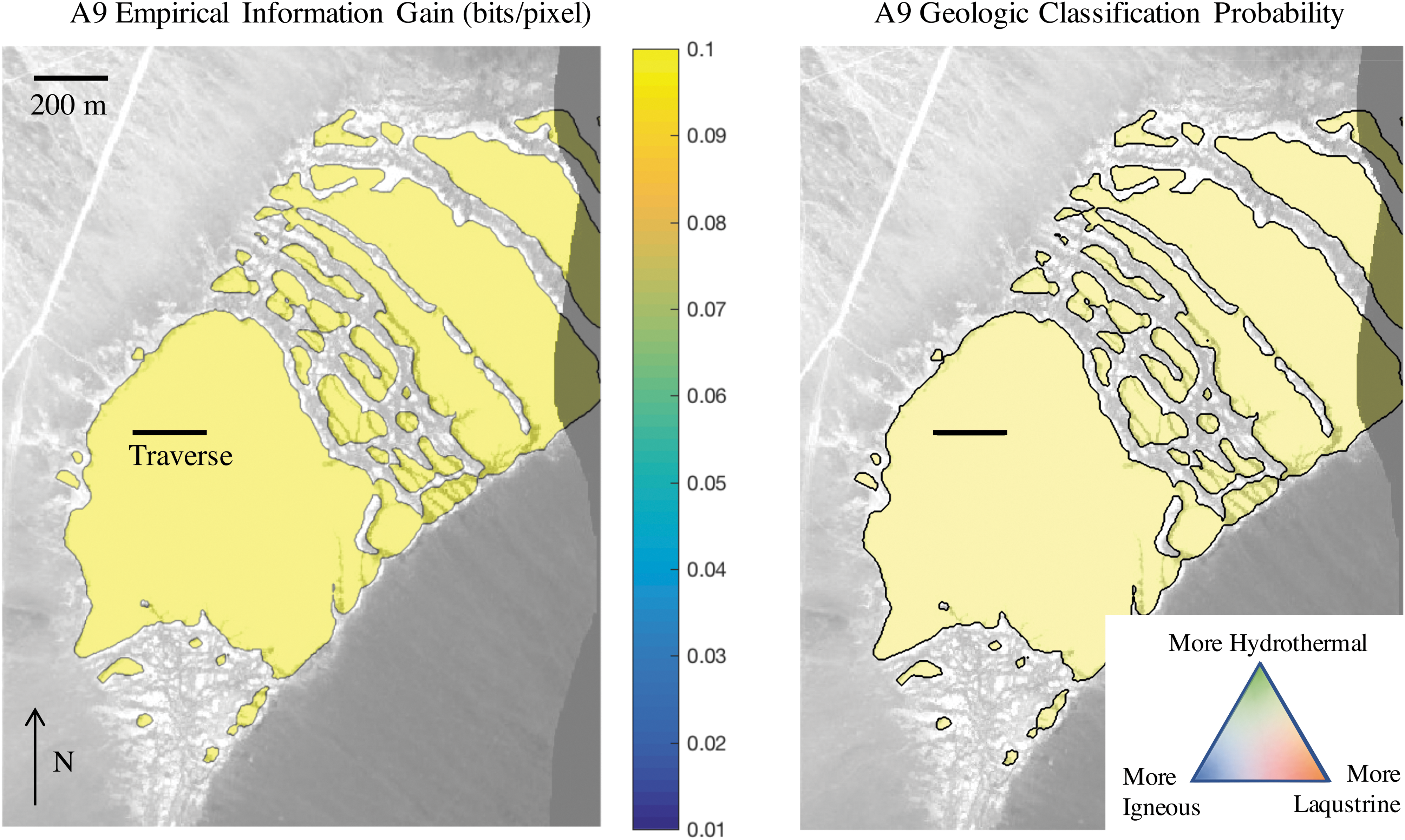
Left: Improvement in posterior entropy (bits per location) calculated for traverse A9. Right: Change in posterior classification probabilities for three of the Objective I geologic classes.

Figure 13 shows a more interesting case where the traverse crosses a boundary between two units. Traverse A8, across the Opal or Chalcedony region, moves from an area dominated by Alunite alteration to one containing hydrated silica (Swayze et al., 2014). The classification is more diverse; the southwest area is more consistent with hydrothermal alteration than the eastern side. These two units are also distinct in the original Ashley and Abrams alteration maps (Ashley and Abrams, 1980; Swayze et al., 2014). The eastern side is associated with silicified minerals, though Objective I does not discriminate beyond the fact that they are hydrothermally altered. These silicified minerals are also highly consistent with an igneous formation process. In contrast, Objective II is specifically tuned to the question of different alteration zones. The right panels of Fig. 13 show traverse results calculated with respect to Objective II. Information gain is lower overall due to the greater intrinsic ambiguity between minerals and alteration zones, reflected in the higher α value and the more consistency possibilities in the conditional probability matrix. In other words, the in situ explorer gets a lower bit yield per measurement for this subtle investigation and must acquire more spectra to achieve the same map certainty. The lower right panel shows the posterior classification; a slight tint indicates a tenuous classification favoring silicified minerals. This categorization is consistent with the Ashley and Abrams map (Ashley and Abrams, 1980).

FIG. 13.

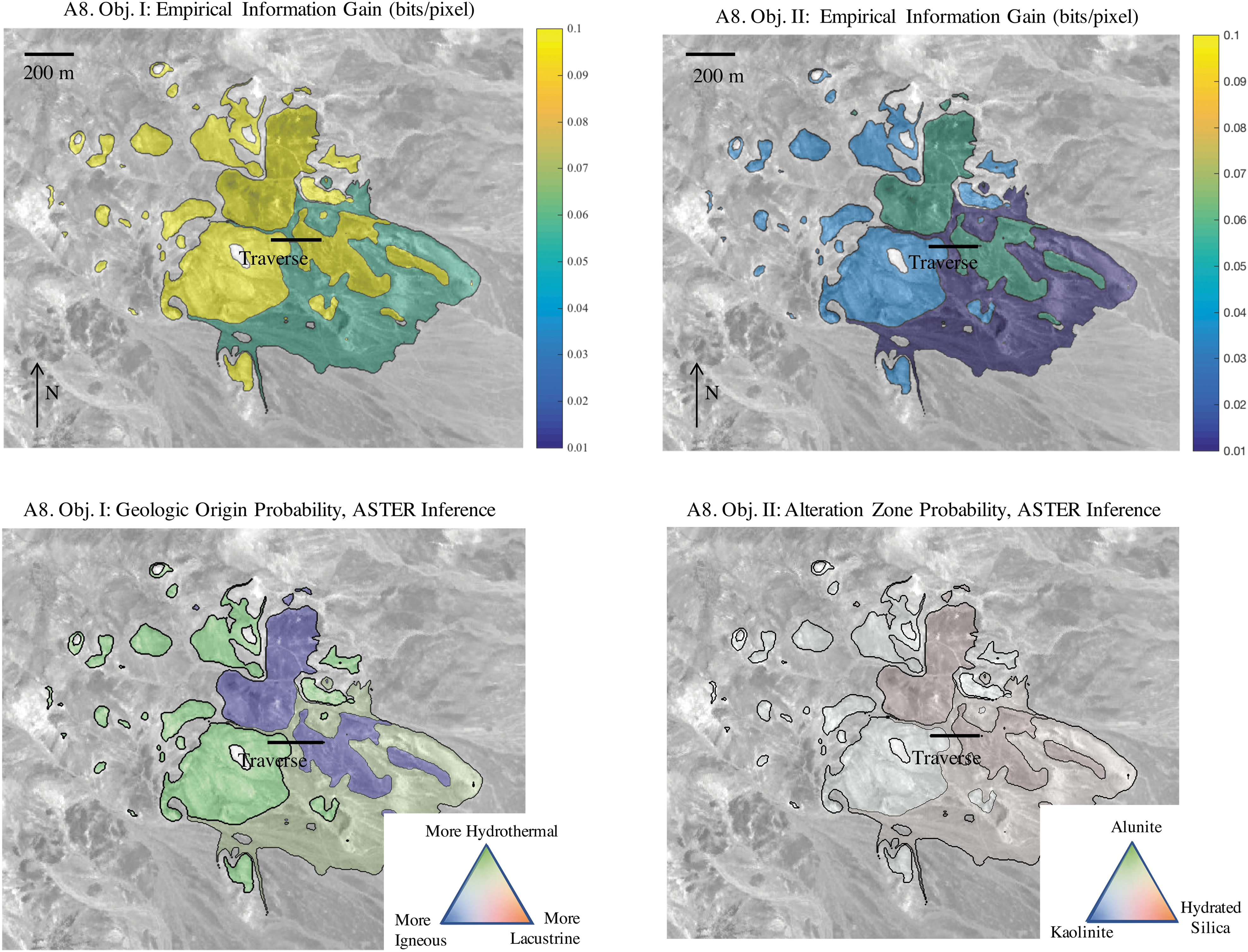
Top: improvement in posterior entropy (bits per location) calculated for the traverse A8, Opal or Chalcedony, for Objectives I (left) and II (right). Bottom: Change in posterior classification probabilities for Objectives I and II.

Figures 14 and 15 show a partitioned model. In this approach, all spectra contribute equally to the classification of the units that contain them; no remote sensing data is used. The left and right panels of Fig. 14 show the change in classification probabilities for traverses across sites A4 and A8 of the western region. These two classification maps are broadly consistent, but the traverses at the sites cross different geologic units leading to different map updates. For reference, the rectangular insets show the area appearing in the prior remote sensing figures. The green area in the left panel is generally correct, but the blue area in the right panel is not consistent with field experience. We emphasize the blue coloration in this figure does not indicate that this region is actually classified as igneous in origin but simply that it becomes more consistent with the igneous classification after the traverse. In fact, the geologic unit is largely hydrothermal with virtually no igneous rock; the model extrapolates incorrectly based on only a glancing intersection of the traverse near an unrepresentative edge. This underscores the dangers of presuming class uniformity over large areas, particularly with pre-segmented regions devised in advance of data collection. Figure 15 compares the same two traverses but calculated with respect to Objective II (alteration zones) and using the prepartitioning of Swayze et al. (2014). Here there is a minor discrepancy; the two traverses lead to different labels for a thin strip classified as kaolinite by A4 but as hydrated silica by A8. The latter is more consistent with Swayze et al. (2014). The incorrect classification implied by traverse A4 comes from a tiny isolated portion of the unit, from which the A4 traverse acquires a small number of spectra. In contrast, A8 crosses a more central location in the unit, acquiring far more spectra and achieving the most reliable classification.

FIG. 14.

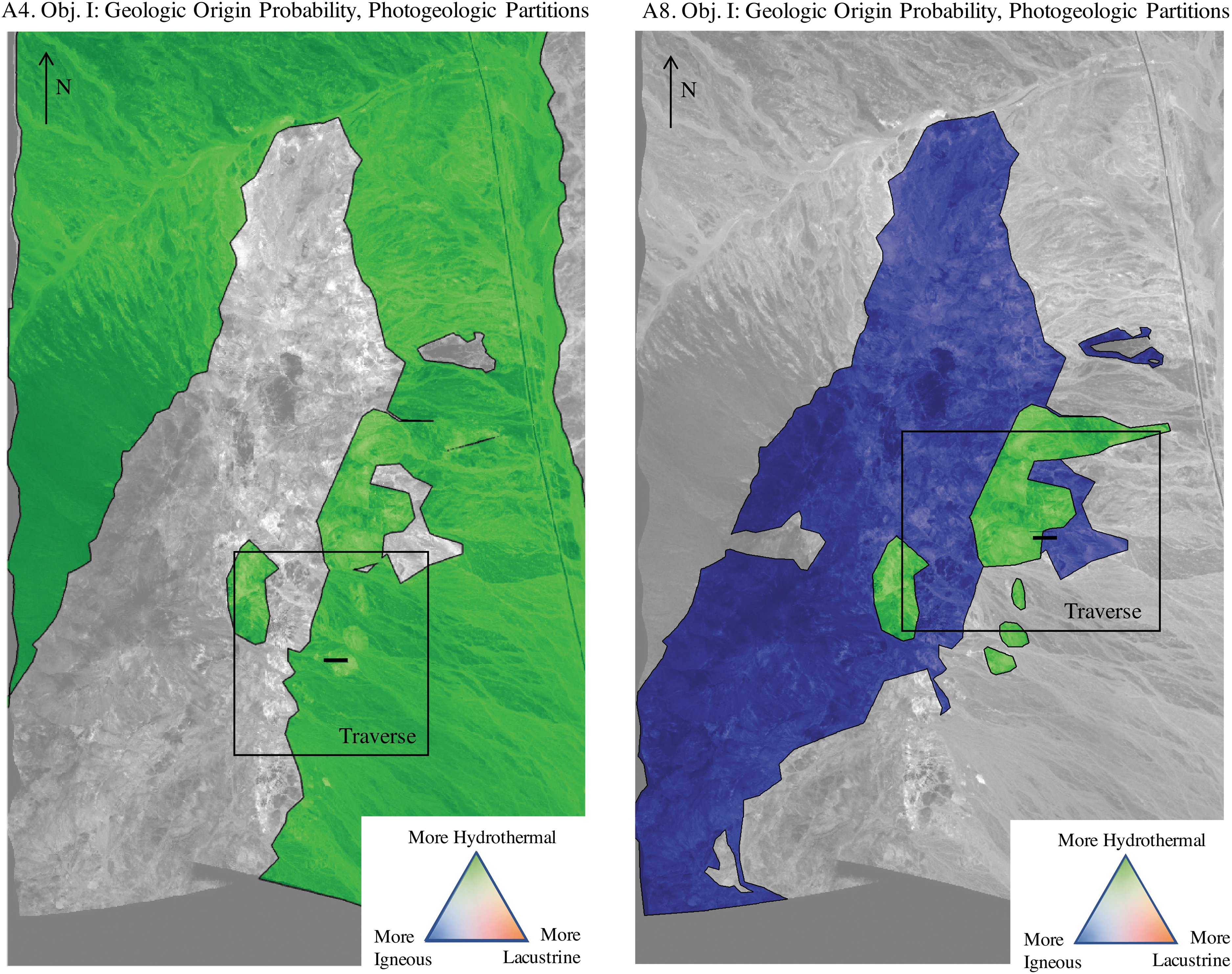
Inferring geologic origin using predefined spatial partitions. Left: Change in geologic origin classification labels after assimilating spectra from traverse A4. The rectangle indicates the inset zoomed-in region of Fig. 11 for reference. Right: Change in geologic origin labels after assimilating spectra from traverse A8. The rectangle indicates the extent of Fig. 13.

FIG. 15.

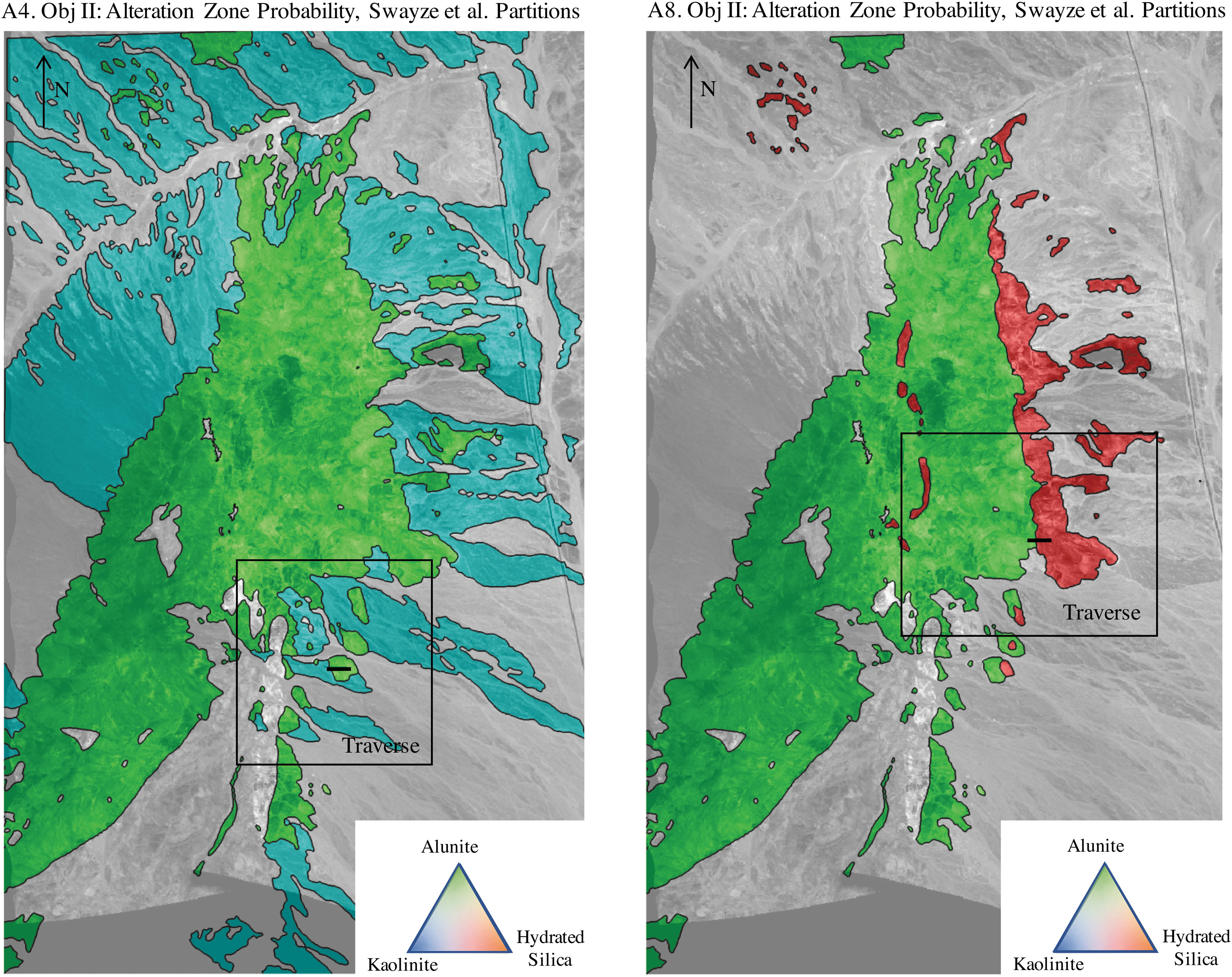
Inferring geologic origin using the alteration units of Swayze et al. (2014). Left: Change in alteration zone classification labels after assimilating spectra from Traverse A4. The rectangle indicates the inset zoomed-in region of Fig. 11 for reference. Right: Change in alteration zone labels after assimilating spectra from Traverse A8. The rectangle indicates the extent of Fig. 13.

While the precise borders differ, classifications based on partitions are generally consistent with maps derived from remote sensing. However, the remote sensing results appear more robust and agree better with conventional interpretations. We attribute this to several factors. First, the remote sensing–based regions are smaller and more appropriate to the level of homogeneity implied by small α values. Second, the remote sensing partitions arise from the ASTER observations at specific pixels and are tied directly to data actually observed at each location. Finally, learning β values provides some additional slack in the model that helps prevent overconfident extrapolations. This carries lessons for future models. We see significant additional benefits of incorporating remote sensing data, even if the measurements themselves are ambiguous on their own. Additionally, it appears safer to oversegment geologic maps with extra boundaries, which helps prevent overconfident extrapolations of geologic classes over wide areas.

4. Discussion

The study offers several specific contributions. First, we formalize the science traceability relationships from an ad hoc STM into a rigorous probabilistic model. This enables hypothesis-driven exploration with quantitative claims that are objectively verifiable and related mathematically to the measurements made by the robot. It contrasts with much adaptive sensing research that focuses on directly measurable quantities. Instead, our approach respects the fundamental investigation questions, in a fashion more appropriate to searches by multiple complementary sensors for abstract or subtle derived geophysical hypotheses. Formalizing hypotheses (as maps) and their relationship to raw data (as a measurement model) permits principled statistical inference and experimental design with direct traceability to mission objectives. We show how to assign model parameters using appropriate combinations of analyst domain knowledge, logical consistency relationships, and statistical learning from training data to fit the remaining free parameters. The resulting system reproduces conventional geologic interpretations of the Cuprite site in two different investigation scenarios.

Our second contribution is the use of partitioning and remote sensing methods to propagate information spatially. Capturing spatial relationships is critical for planning autonomous robotic exploration, since it bears on the information value of future measurements given the data already collected. This allows robotic activity plans to be optimized by computer, playing to the strengths of the automated half of the co-robotic pair. It also allows the system to react to unanticipated events that occur while the robot is out of touch with users. For example, delays in navigation are common due to hazard avoidance (Thompson et al., 2011) or unanticipated air/sea currents. Robots that understand the hypotheses under study, and their manifestation at different locations, can recover from navigation or execution delays by optimizing a fallback strategy. They can exploit resource surpluses in a similar fashion (Thompson et al., 2011). Another benefit for exploration efficiency is to overcome requirements for tedious close interaction with each field robot. Probabilistic maps can communicate the latest objectives simply and intuitively, defining the appropriate behaviors without the tedium of low-level action planning.

Third, the Cuprite experiments provide the first experimental evidence for an intuitive but hitherto undemonstrated claim: that the distribution of spectroscopic information is highly dependent on investigation objectives. The simple coarse geologic classification (Objective I) is relatively easy, and any location within a unit soon results in an appropriate classification. The relationships between minerals and geologic class are definitive, with relatively few ambiguous minerals and a low appearance of mutually inconsistent minerals as indicated by empirical α values. In contrast, Objective II is subtler; it requires many measurements (and ideally, multiple kinds of minerals per unit) to overcome observation ambiguity. This is most pronounced when extrapolating spatially using remote sensing data, where the investigation must also battle the uncertainty in the interpretation of multiband measurements. Other things equal, certainty in the identification increases with the number of spectral channels (Swayze et al., 2003). Rigorous tracking of these conditional distributions, and propagation of these uncertainties to the end maps, is a key feature of our approach. We do find a strong statistical link between measured spectra, mineralogy, and the geologic unit classes. This is not self-evident because geologists form origin and alteration classifications from countless other features such as local morphology, elevation, the wide-area three-dimensional structure of different strata, and domain knowledge. The ability to corroborate these insights with just a few spectra makes the Cuprite data set an excellent test case for our study.

This general approach can drive automatic decision-making for measurement and downlink wherever an agent must explore an environment while balancing data collection and resource costs against science information gain. Existing path and observation planners able to use these models include the P-SPIEL approach of Singh et al. (2009); branch and bound algorithms such as those in Binney and Sukhatme (2012), or Hollinger and Sukhatme (2014); the optimization strategy of Candela et al. (2017); and the sampling-based planner of Arora et al. (2017). The model applies to many different exploration problems including time series sampling, selective in situ sampling within a rover arm workspace, and allocation of orbital observations. Operators can guide the process in multiple ways, such as by defining the map and probabilistic model, by manually revising the robot's belief state, or by imposing constraints such as resource limits, goal waypoints, or required measurements.

A wide range of planetary missions might benefit from some degree of science autonomy. Here we show a test case involving remote exploration of hydrothermal systems, which are important sites for biopreservation on Mars. More generally, the techniques apply to other time-limited remote astrobiology investigations, the science return of which scales with their ability to fully utilize the in situ instruments during long periods between communications. Naturally, future missions will be more challenging than the Cuprite case study. The most interesting astrobiology questions relate to highly localized phenomena—organics or evidence of life. These would likely require more than just a geologic map, remote sensing, and a profiling spectrometer. Instead, they would require a full imaging spectrometer at orbital spatial resolution coupled with in situ imaging spectroscopy and perhaps microscale imaging as well. Maps would be less accurate than the terrestrial case. This research aims to help establish a mathematical foundation for science autonomy that could generalize to these more complex and dynamic missions. Recent robotics advances in the areas of long-duration autonomy and long-distance mobility illustrate the need for human co-robot exploration leveraging adaptive data collection. Robots can now spend days in the field and travel multiple kilometers per single uplink/downlink communications cycle. These platforms can deploy instruments over wide areas, augmenting human explorers and acting on their behalf when appropriate. Our future work will continue to investigate this problem as a venue to refine the relationship between human scientists and robotic explorers, ultimately increasing the productivity and yield of both.

5. Conclusion

A case study of Cuprite Hills, Nevada, quantifies the information gain of different in situ spectroscopic measurements with respect to more abstract questions about hydrothermal alteration, in the context of prior knowledge and ASTER remote sensing data. We demonstrate efficient estimation of model parameters and automatic inference of posterior classifications consistent with prior literature. The case study gives insight into the exploration process, as well as the spatial distribution of spectroscopic information at Cuprite, a site of significant historical and geologic value.

Footnotes

Acknowledgments

We thank the members of the AVIRIS-NG team who participated in data acquisition and analysis, including Michael Eastwood and Sarah Lundeen. We thank Raymond Kokaly (United States Geographical Survey) for his counsel. AVIRIS-NG is sponsored by the National Aeronautics and Space Administration (NASA) Earth Science Division. This research was carried out at the Jet Propulsion Laboratory, California Institute of Technology, under a contract with the National Aeronautics and Space Administration. This project was supported by the National Science Foundation's National Robotics Initiative, Award No. 1526667. Gregg Swayze's participation was made possible by synergistic projects at the United States Geological Survey. Any use of trade, firm, or product names in this publication is for descriptive purposes only and does not imply endorsement by the U.S. Government.

Abbreviations Used

References

Abrams

M.J.

, Ashley

R.P.

, Rowan

L.C.

, Goetz

A.F.

, and Kahle

A.B.

(1977) Mapping of hydrothermal alteration in the Cuprite mining district, Nevada, using aircraft scanner images for the spectral region 0.46 to 2.36 μm. Geology, 5:713–718.

Achanta

, Shaji

, Smith

, Lucchi

, Fua

, and Süsstrunk

(2012) SLIC superpixels compared to state-of-the-art superpixel methods. IEEE Trans Pattern Anal Mach Intell, 34:2274–2282.

Albers

and Stewart

(1972) Geology and Mineral Deposits of Esmeralda County, Nevada, Bulletin 78, Nevada Bureau of Mines and Geology, Reno, NV.

Arora

, Fitch

, and Sukkarieh

(2017) An approach to autonomous science by modeling geological knowledge in a Bayesian framework. In IEEE/RSJ International Conference on Intelligent Robots and Systems (IROS), IEEE, Piscataway, NJ, doi:10.1109/IROS.2017.8206230.

Ashley

and Abrams

(1980) Alteration Mapping Using Multispectral Images, Cuprite Mining District, Esmeralda County, Nevada, Open File Report 80–367, U.S. Geological Survey, Reston, VA.

Bekker

D.L.

, Thompson

D.R.

, Abbey

W.J.

, Cabrol

N.A.

, Francis

, Manatt

K.S.

, Ortega

K.F.

, and Wagstaff

K.L.

(2014) Field demonstration of an instrument performing automatic classification of geologic surfaces. Astrobiology, 14:486–501.

Bernardo

(1979) Expected information as expected utility. Ann Stat, 7:686–690.

Binney

and Sukhatme

G.S.

(2012) Branch and bound for informative path planning. In IEEE International Conference on Robotics and Automation, IEEE, Piscataway, NJ, doi:10.1109/ICRA.2012.6224902.

Bramble

M.S.

, Mustard

J.F.

, and Salvatore

M.R.

(2017) The geological history of northeast Syrtis Major, Mars. Icarus, 293:66–93.

10.

Candela

, Thompson

D.R.

, Dobrea

E.N.

, and Wettergreen

D.S.

(2017) Planetary robotic exploration driven by science hypotheses for geologic mapping. In IEEE/RSJ International Conference on Intelligent Robots and Systems (IROS), IEEE, Piscataway, NJ, doi:10.1109/IROS.2017.8206231.

11.

Chaloner

and Verdinelli

(1995) Bayesian experimental design: a review. Stat Sci, 10:273–304.

12.

Chien

S.A.

, Sherwood

, Tran

, Cichy

, Rabideau

, Castano

, Davies

, Mandl

, Trout

, Shulman

, and Boyer

(2005) Using autonomy flight software to improve science return on Earth observing one. Journal of Aerospace Computing, Information, and Communication, 2:196–216.

13.

Clark

, Swayze

, Murchie

, Seelos

, and Viviano-Beck

(2015) Mineral and other materials mapping of CRISM data with Tetracorder 5 [abstract 2410]. In 46^th Lunar and Planetary Science Conference, Lunar and Planetary Institute, Houston.

14.

Clark

R.N.

, Swayze

G.A.

, Livo

K.E.

, Kokaly

R.F.

, Sutley

S.J.

, Dalton

J.B.

, McDougal

R.R.

, and Gent

C.A.

(2003) Imaging spectroscopy: Earth and planetary remote sensing with the USGS Tetracorder and expert systems. J Geophys Res: Planets, 108, doi:10.1029/2002JE001847.

15.

Clark

R.N.

, Swayze

G.A.

, Leifer

, Livo

K.E.

, Kokaly

, Hoefen

, Lundeen

, Eastwood

, Green

R.O.

, Pearson

, Sarture

, McCubbin

, Roberts

, Bradley

, Steele

, Ryan

, Dominguez

, and the Airborne Visible/Infrared Imaging Spectrometer (AVIRIS) Team. (2010) A Method for Quantitative Mapping of Thick Oil Spills Using Imaging Spectroscopy, U.S. Geological Survey Open-File Report 1167, U.S. Geological Survey, Reston, VA.

16.

Cover

T.M.

and Thomas

J.A.

(2006) Elements of Information Theory,, 2 ^nd ed., Wiley-Interscience, Hoboken, NJ.

17.

Doran

, Thompson

D.R.

, and Estlin

T.A.

(2016) Precision instrument targeting via image registration for the Mars 2020 rover. In Proceedings of the Twenty-Fifth International Joint Conference on Artificial Intelligence, ICJAI 2016, AAAI Press,. Palo Alto, CA, pp 3352–3358.

18.

Estlin

T.A.

, Bornstein

B.J.

, Gaines

D.M.

, Anderson

R.C.

, Thompson

D.R.

, Burl

, Castaño

, and Judd

(2012) Aegis automated science targeting for the MER Opportunity rover. ACM Transactions on Intelligent Systems and Technology (TIST), 3, doi:10.1145/2168752.2168764.

19.

Farmer

J.D.

(2000) Hydrothermal systems: doorways to early biosphere evolution. GSA Today, 10:1–9.

20.

Fink

, Dohm

J.M.

, Tarbell

M.A.

, Hare

T.M.

, and Baker

V.R.

(2005) Next-generation robotic planetary reconnaissance missions: a paradigm shift. Planet Space Sci, 53:1419–1426.

21.

Fong

(2017) Interactive Exploration Robots: Human-Robotic Collaboration and Interactions, NASA Ames Research Center Technical Report ARC-E-DAA-TN44701, Document 20170009903, NASA Ames Research Center, Moffett Field, CA.

22.

Francis

, Estlin

, Doran

, Johnstone

, Gaines

, Verma

, Burl

, Frydenvang

, Montaño

, Wiens

, Schaffer

, Gasnault

, DeFlores

, Blaney

, and Bornstein

(2017) Aegis autonomous targeting for ChemCam on Mars Science Laboratory: deployment and results of initial science team use. Science Robotics, 2, doi:10.1126/scirobotics.aan4582.

23.

Goetz

A.F.

and Srivastava

(1985) Mineralogical mapping in the Cuprite mining district, Nevada. In Proceedings of the Airborne Imaging Spectrometer (AIRS) Data Analysis Workshop, Jet Propulsion Laboratory Publication 85-41, Jet Propulsion Laboratory, California Institute of Technology, Pasadena, CA, pp. 22–29.

24.

Green

R.O.

, Eastwood

M.L.

, Sarture

C.M.

, Chrien

T.G.

, Aronsson

, Chippendale

B.J.

, Faust

J.A.

, Pavri

B.E.

, Chovit

C.J.

, Solis

, Olah

M.R.

, and Williams

(1998) Imaging spectroscopy and the Airborne Visible/Infrared Imaging Spectrometer (AVIRIS). Remote Sens Environ, 65:227–248.

25.

Hamlin

, Green

, Mouroulis

, Eastwood

, Wilson

, Dudik

, and Paine

(2011) Imaging spectrometer science measurements for terrestrial ecology: AVIRIS and new developments. In 2011 IEEE Aerospace Conference, IEEE, Piscataway, NJ, doi:10.1109/AERO.2011.5747395.

26.

Hock

A.N.

, Cabrol

N.A.

, Dohm

J.M.

, Piatek

, Warren-Rhodes

, Weinstein

, Wettergreen

D.S.

, Grin

E.A.

, Moersch

, Cockell

C.S.

, Coppin

, Ernst

, Fisher

, Hardgrove

, Marinangeli

, Minkley

, Ori

G.G.

, Waggoner

, Wyatt

, Smith

, Thompson

, Wagner

, Jonak

, Stubbs

, Thomas

, Pudenz

, and Glasgow

(2007) Life in the Atacama: a scoring system for habitability and the robotic exploration for life. J Geophys Res: Biogeosciences, 112, doi:10.1029/2006JG000321.

27.

Hollinger

G.A.

and Sukhatme

G.S.

(2014) Sampling-based robotic information gathering algorithms. Int J Rob Res, 33:1271–1287.

28.

Iwasaki

and Tonooka

(2005) Validation of a crosstalk correction algorithm for ASTER/SWIR. IEEE Trans Geosci Remote Sens, 43:2747–2751.

29.

Jasper

L.E.Z

. and Xaypraseuth

(2017) Data production on past and future NASA missions. In 2017 IEEE Aerospace Conference, IEEE, Piscataway, NJ, doi:10.1109/AERO.2017.7943918.

30.

Kruse

, Keirein-Young

, and Boardman

(1990) Mineral mapping at Cuprite, Nevada with a 64-channel imaging spectrometer. Photogramm Eng Remote Sensing, 56:83–92.

31.

Kruse

F.A.

and Perry

S.L.

(2009) Improving multispectral mapping by spectral modeling with hyperspectral signatures. J Appl Remote Sens, 3:033504.

32.

Lindley

(1956) On the measure of information provided by an experiment. The Annals of Mathematical Statistics, 27:986–1005.

33.

Lorenz

R.D.

and Cabrol

N.A.

(2018) Onboard science insights and vehicle dynamics from scale-model trials of the Titan Mare Explorer (TIME) capsule at Laguna Negra, Chile. Astrobiology, 18:607–618.

34.

McGuire

P.C.

, Bonnici

, Bruner

, Gross

, Ormö

, Smosna

, Walter

, and Wendt

(2014) The cyborg astrobiologist: matching of prior textures by image compression for geological mapping and novelty detection. International Journal of Astrobiology, 13:191–202.

35.

McLennan

, Sephton

, Allen

, Allwood

, Barbieri

, Beaty

, Boston

, Carr

, Grady

, Grant

, Heber

V.S.

, Herd

C.D.K.

, Hofmann

, King

, Mangold

, Ori

G.G.

, Rossi

A.P.

, Raulin

, Ruff

S.W.

, Sherwood Lollar

, Symes

, and Wilson

M.G.

(2012) Planning for Mars returned sample science: final report of the MSR End-To-End International Science Analysis Group (E2E-ISAG). Astrobiology, 12:175–230.

36.

MEPAG Next Decade Science Analysis Group. (2008) Science priorities for Mars sample return. Astrobiology, 8:489–535.

37.

Michalski

J.R.

, Dobrea

E.Z.N.

, Niles

P.B.

, and Cuadros

(2017) Ancient hydrothermal seafloor deposits in Eridania Basin on Mars. Nat Commun, 8, doi:10.1038/ncomms15978.

38.

Milliken

, Grotzinger

, and Thomson

(2010) Paleoclimate of Mars as captured by the stratigraphic record in Gale Crater. Geophys Res Lett, 37, doi:10.1029/2009GL041870.

39.

Paninski

(2005) Asymptotic theory of information-theoretic experimental design. Neural Comput, 17:1480–1507.

40.

Rowan

L.C.

, Wetlaufer

, Goetz

A.F.

, and Stewart

(1974) Discrimination of Rock Types and Detection of Hydrothermally Altered Areas in South-Central Nevada by the Use of Computer-Enhanced ERTS Images, Professional Paper 883, U.S. Geological Survey, Reston, VA.

41.

Rowan

L.C.

, Hook

S.J.

, Abrams

M.J.

, and Mars

J.C.

(2003) Mapping hydrothermally altered rocks at Cuprite, Nevada, using the Advanced Spaceborne Thermal Emission and Reflection Radiometer (ASTER), a new satellite-imaging system. Econ Geol, 98:1019–1027.

42.

Shewry

M.C.

and Wynn

H.P.

(1987) Maximum entropy sampling. J Appl Stat, 14:165–170.

43.

Singh

, Krause

, and Kaiser

W.J.

(2009) Nonmyopic adaptive informative path planning for multiple robots. In 21^st International Joint Conference on Artificial Intelligence (IJCAI), Morgan Kaufmann, San Francisco, CA, pp. 1043–1050.

44.

Squyres

, Arvidson

R.E.

, Ruff

, Gellert

, Morris

, Ming

, Crumpler

, Farmer

, Des Marais

, Yen

, McLennan

S.M.

, Calvin

, Bell

J.F.

, III, Clark

B.C.

, Wang

, McCoy

T.J.

, Schmidt

M.E.

, and de Souza

P.A.

Jr . (2008) Detection of silica-rich deposits on Mars. Science, 320:1063–1067.

45.

Swayze

G.A.

, Clark

R.N.

, Goetz

A.F.

, Chrien

T.G.

, and Gorelick

N.S.

(2003) Effects of spectrometer band pass, sampling, and signal-to-noise ratio on spectral identification using the tetracorder algorithm. J Geophys Res: Planets, 108, doi:10.1029/2002JE001975.

46.

Swayze

G.A.

, Clark

R.N.

, Goetz

A.F.

, Livo

K.E.

, Breit

G.N.

, Kruse

F.A.

, Sutley

S.J.

, Snee

L.W.

, Lowers

H.A.

, Post

J.L.

, Stoffregen

R.E.

, and Ashley

R.P.

(2014) Mapping advanced argillic alteration at Cuprite, Nevada, using imaging spectroscopy. Econ Geol, 109:1179–1221.

47.

Thompson

D.R.

, Wettergreen

D.S.

, and Peralta

F.J.C.

(2011) Autonomous science during large-scale robotic survey. Journal of Field Robotics, 28:542–564.

48.

Thompson

D.R.

, Bornstein

B.J.

, Chien

S.A.

, Schaffer

, Tran

, Bue

B.D.

, Castaño

, Gleeson

D.F.

, and Noell

(2013) Autonomous spectral discovery and mapping onboard the EO-1 spacecraft. IEEE Trans Geosci Remote Sens, 51:3567–3579.

49.

Thompson

D.R.

, Flannery

D.T.

, Lanka

, Allwood

A.C.

, Bue

B.D.

, Clark

B.C.

, Elam

W.T.

, Estlin

T.A.

, Hodyss

R.P.

, Hurowitz

J.A.

, Liu

, and Wade

L.A.

(2015a) Automating X-ray fluorescence analysis for rapid astrobiology surveys. Astrobiology, 15:961–976.

50.

Thompson

D.R.

, Gao

B.C.

, Green

R.O.

, Roberts

D.A.

, Dennison

P.E.

, and Lundeen

S.R.

(2015b) Atmospheric correction for global mapping spectroscopy: ATREM advances for the HyspIRI preparatory campaign. Remote Sens Environ, 167:64–77.

51.

Thompson

D.R.

, Wettergreen

, Foil

, Furlong

, and Kiran

A.R.

(2015c) Spatiospectral exploration combining in situ and remote measurements. In Twenty-Ninth AAAI Conference on Artificial Intelligence, AAAI Press, Palo Alto, CA, pp 3679–3685.

52.

Thompson

D.R.

, Hochberg

E.J.

, Asner

G.P.

, Green

R.O.

, Knapp

D.E.

, Gao

B.C.

, Garcia

, Gierach

, Lee

, Maritorena

, and Fick

(2017) Airborne mapping of benthic reflectance spectra with Bayesian linear mixtures. Remote Sens Environ, 200:18–30.

53.

Thompson

D.R.

, Boardman

J.W.

, Eastwood

M.L.

, Green

R.O.

, Haag

J.M.

, Mouroulis

, and Van Gorp

B.E.

(2018) Imaging spectrometer stray spectral response: in-flight characterization, correction, and validation. Remote Sens Environ, 204:850–860.

54.

van den Berg

, Curtis

, and Trampert

(2003) Optimal nonlinear Bayesian experimental design: an application to amplitude versus offset experiments. Geophys J Int, 155:411–421.

55.

Van Der Meer

(2004) Analysis of spectral absorption features in hyperspectral imagery. Int J Appl Earth Obs Geoinf, 5:55–68.

56.

Woods

, Shaw

, Tidey

, Van Pham

, Simon

, Mukherji

, Maddison

, Cross

, Kisdi

, Tubby

, Visentin

, and Chong

(2014) Seeker autonomous long-range rover navigation for remote exploration. Journal of Field Robotics, 31:940–968.

57.

Wray

, Noe Dobrea

, Arvidson

, Wiseman

, Squyres

, McEwen

, Mustard

, and Murchie

(2009) Phyllosilicates and sulfates at Endeavour Crater, Meridiani Planum, Mars. Geophys Res Lett, 36, doi:10.1029/2009GL040734.