A Physical Modeling Approach for Higher Plant Growth in Reduced Gravity Environments

Abstract

Including plants in bioregenerative life-support systems enables simultaneous food production and water and air recycling, while closing cycles for water, oxygen, nitrogen, and carbon. To understand and predict higher plant behavior for a wide range of environmental conditions, including reduced gravity levels, a mechanistic physical model is being developed. The emphasis is set on the influence of gravity levels and forced convection on higher plant leaf gas exchanges, which are altered by reduction of free convection in lower gravity environments, such as microgravity or martian and lunar gravities. This study highlights the significance of understanding leaf boundary layer limitations and ultimately will lead to complete mechanistic modeling of mass and energy balances on plant growth in reduced gravity environments.

1. Introduction

A closed-loop life-support system (LSS) comprises several functions: atmosphere regeneration, waste treatment, and water recycling (Mitchell, 1994; Eckart, 1996; Anderson et al., 2015). In the domain of space exploration, one major constraint is the payload mass and resupply costs for long-term exploration or permanent habitation LSSs (Anderson et al., 2015). To improve the closure of a human LSS, and because physicochemical technologies alone are not sufficient, it becomes necessary to include biological compartments, at least at the food production level, such as a photoautotrophic compartment, including higher plants and microalgae (Ewert et al., 2002; Drayer and Howard, 2014; Fu et al., 2016), for in situ food production (Wheeler, 2004, 2011, 2017; Furfaro et al., 2016), complementary to water recycling, O₂ production, and CO₂ removal. By definition, the bioregenerative LSS is a loop system so that all functions are strongly intertwined and interact with each other (Wheeler, 2003; Clauwaert et al., 2015; Dong et al., 2017), and since there is no buffer effect in space, slight variations in environmental parameters can dramatically affect the whole loop. To use bioregenerative LSSs to sustain human beings off Earth, a complete understanding of the dynamical functioning of the system is required. This can be achieved with a mechanistic modeling approach based on basic principles of element conservation, chemical and biological kinetics, and a thorough understanding of the coupling phenomena between physical and biochemical determinants.

In particular, the influence of space environmental conditions, such as reduced gravity, on plant growth mechanisms needs to be addressed. Major effects of impaired gravity on plant growth occur on the orientation of roots, on migration of sap within the stem, and on gas exchanges at the leaf surface (Poulet et al., 2016).

Indeed, a lower gravity level also means lower free convection velocities (Kitaya et al., 2001, 2003a; Hirai and Kitaya, 2009), leading to increased boundary layers of stagnant air forming around plant leaves, thus reducing gas exchanges at the leaf surface and photosynthesis (Kitaya et al., 2000, 2003b, 2004; Boulard et al., 2002; Kitaya, 2016). Long-duration tests on the International Space Station have shown that with adequate ventilation, photosynthesis rates are similar to those on Earth (Monje et al., 2000, 2005), but to be able to predict plant behavior for a wide range of parameters, suboptimal cases must be studied. Indeed, in case of failure of one system, the model should predict, for example, how this will impact oxygen and food production or how much time the crew has left before losing parts of or the whole crop production.

The frame of this work is the Micro-Ecological Life-Support System Alternative (MELiSSA) project of the European Space Agency (ESA), a closed-loop artificial ecosystem that is inspired from a lake ecosystem comprising five compartments (Hendrickx et al., 2006; Lasseur et al., 2011) and for which modeling efforts of the higher plant compartment are still ongoing (Hézard, 2012; Poulet et al., 2016, 2017). The initial plant growth model was based on mass balance aspects while addressing limitations of current, existing agronomy models (Hézard et al., 2010).

In this article, emphasis is set on the influence of gravity levels such as microgravity and Earth, Mars, and lunar gravities, as well as the influence of free and forced convection on the leaf boundary layer thickness, higher plant gas exchanges, and biomass production. The link between gas exchanges and the plant energy balance is also discussed.

2. Materials and Methods

2.1. Overall structure of the higher plant growth model

The higher plant growth model encompasses four modules corresponding to four study levels (Fig. 1): the environmental module accounts for variations of process parameters at the surrounding environmental scale; the morphological module includes structural changes at the plant scale; the physical module represents the rate-limiting processes impacting biomass growth at the organ scale; and the biochemical module accounts for metabolic growth equations at the cell scale, including stoichiometric constraints (Hézard, 2012).

FIG. 1.

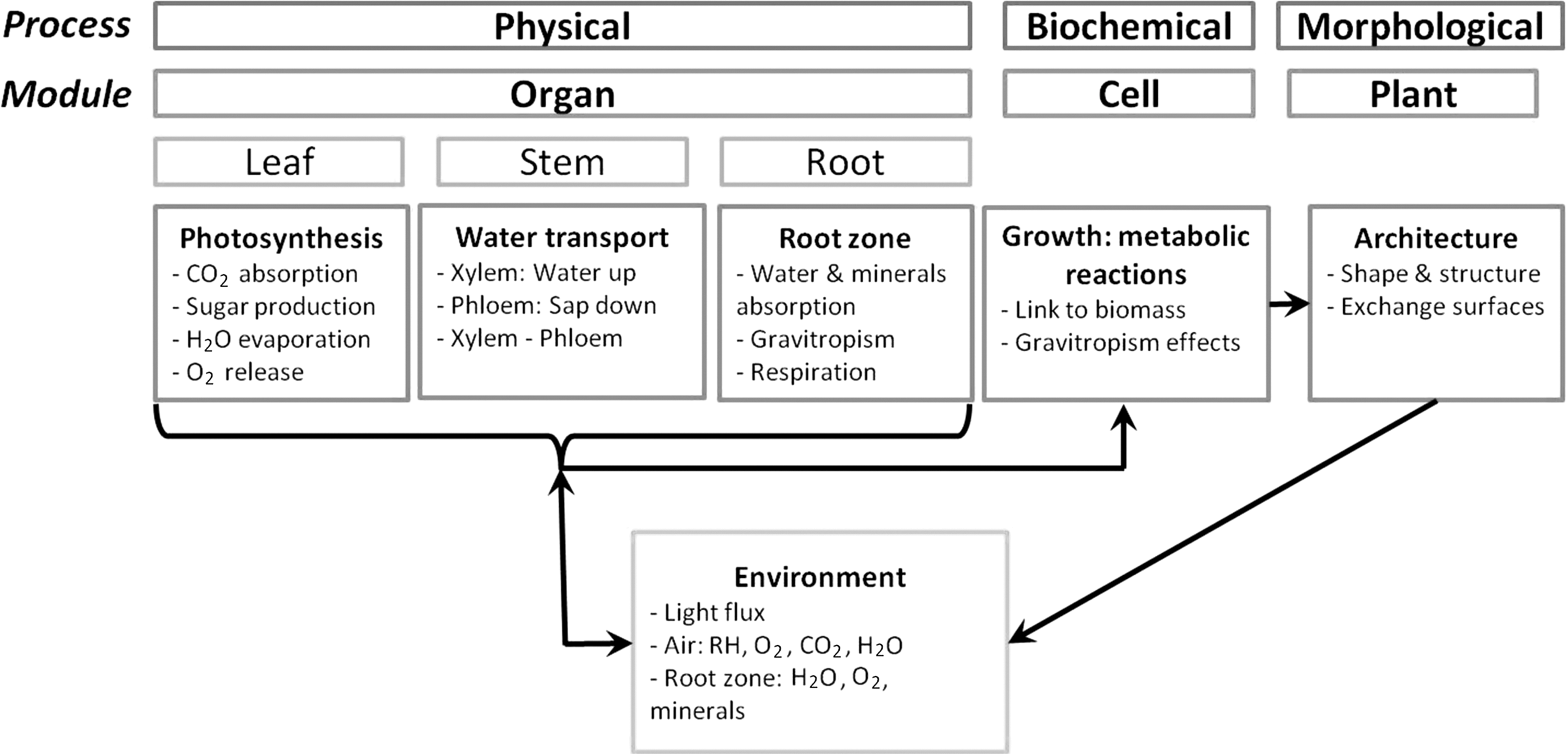
Diagram illustrating the model structure with four main modules: physical, biochemical, morphological, and environmental modules.

This model is built so that it can be adapted to virtually any plant species by entering adequate species-dependent parameters. In a first approach, the higher plant is considered as a circular single leaf, with the leaf area, stem length, and number of vessels within the leaf increasing proportionally with biomass increase. The proportionality coefficients used to compute these morphological traits are species dependent and can be assessed experimentally for the studied species. The leaf area or stem growth will thus differ according to the studied species. These morphological traits are used within physical equations to compute the maximum fluxes for water uptake and transpiration, as well as CO₂ uptake and light interception. To assess the influence of different gravity levels on the physical module, the behavior of gas exchanges must be investigated. The application here is a study of transfer rates at a leaf level, the leaf being considered as a solid horizontal plate, with the surface increasing proportionally with the biomass increase.

The light interception follows the Beer–Lambert law, while the CO₂ uptake and the water transpiration are diffusion equations following Fick's law (Fig. 2), and the water uptake equation is the Poiseuille law. The metabolic description coupled to the kinetic uptake rate of CO₂ derived from the light energy transfer model provides the calculation of metabolic fluxes for lit periods and of instantaneous biomass production rates. These metabolic fluxes are computed using the quantum yield, which is species dependent, especially depending on if the plant is a C3 or a C4 (Ehleringer and Björkman, 1977).

FIG. 2.

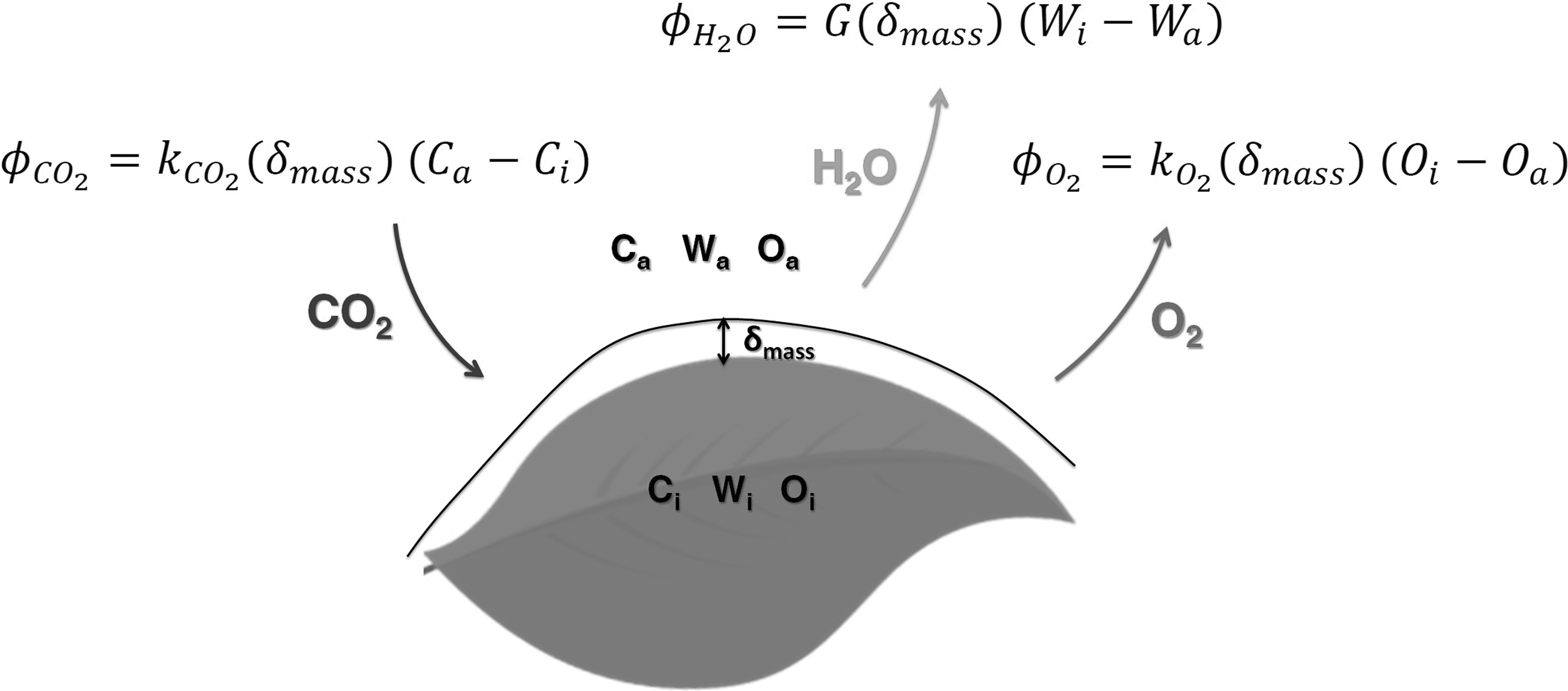
Schematic view of gas exchanges at the leaf surface. ϕ_CO₂ is the CO₂ uptake rate, ϕ_H₂O is the water vapor release (transpiration) rate, and ϕ_O₂ the O₂ production rate; k_CO₂(δ_mass) and k_O₂(δ_mass) are exchange coefficients for, respectively, CO₂ uptake and O₂ release; C_a, W_a, and O_a are, respectively, the external CO₂, water vapor, and O₂ concentrations and C_i, W_i, and O_i are, respectively, the leaf internal CO₂, water vapor, and O₂ concentrations.

Integration along time, accounting for lit and dark periods, leads to biomass production over a given period of time.

2.2. Gas exchanges at the leaf surface

Gas exchanges at the leaf surface between the plant and the atmosphere depend on two diffusion phenomena, one through the leaf's stomata and one through the boundary layer, and on the convection regime around the plant (Lambers et al., 2008; Poulet et al., 2017). The gas exchange equations follow Fick's law of diffusion, with an exchange coefficient and a concentration gradient driving the exchange (Fig. 2).

In the case of CO₂ uptake, the gradient driving the exchange is the difference between the external CO₂ concentration (Ca in Fig. 2) and internal leaf CO₂ concentration (Ci in Fig. 2) (Hézard, 2012). The exchange coefficient (k_CO2(δ_mass) in Fig. 2) is the ratio between the diffusion coefficient for CO₂ D_c and the thickness of the boundary layer δ_mass: \documentclass{aastex}\usepackage{amsbsy}\usepackage{amsfonts}\usepackage{amssymb}\usepackage{bm}\usepackage{mathrsfs}\usepackage{pifont}\usepackage{stmaryrd}\usepackage{textcomp}\usepackage{portland, xspace}\usepackage{amsmath, amsxtra}\usepackage{upgreek}\pagestyle{empty}\DeclareMathSizes{10}{9}{7}{6}\begin{document} \begin{align*}{ k_ { C { O_2 } } } = \; { \frac { { D_c } } { { \delta _ { mass } } } } . \end{align*} \end{document}

For water transpiration, the water partial pressure gradient driving the exchange is the difference between the surface water partial pressure that is considered as saturated at the surface temperature and the atmosphere bulk water partial pressure. In other words, this corresponds to a difference in relative humidity between the inside and the outside of the leaf. The exchange coefficient (G(δ_mass) in Fig. 2) is the leaf conductance, which is a function of the thickness of the mass boundary layer surrounding the leaf.

2.3. Leaf conductance

The total leaf conductance describes the diffusion capacity through the leaf. It is also defined as the inverse of the leaf's resistance to diffusion processes. It is a combination of the two conductances associated with the two diffusion processes occurring at the leaf surface: stomatal conductance and boundary layer conductance. The boundary layer conductance for water is a function of the diffusion coefficient for water vapor D_w, molar water vapor density ρ_mol,w, and thickness of the boundary layer δ_mass (Lambers et al., 2008): \documentclass{aastex}\usepackage{amsbsy}\usepackage{amsfonts}\usepackage{amssymb}\usepackage{bm}\usepackage{mathrsfs}\usepackage{pifont}\usepackage{stmaryrd}\usepackage{textcomp}\usepackage{portland, xspace}\usepackage{amsmath, amsxtra}\usepackage{upgreek}\pagestyle{empty}\DeclareMathSizes{10}{9}{7}{6}\begin{document} \begin{align*} g_w^ { BL } = \; { \frac { { D_w } { \rho _ { mol , w } } } { { \delta _ { mass } } } } . \end{align*} \end{document}

Stomatal conductance is a function of parameters that are plant and species dependent, so it differs from one plant species to another and enables the gas exchange model to be adapted for a specific plant species: \documentclass{aastex}\usepackage{amsbsy}\usepackage{amsfonts}\usepackage{amssymb}\usepackage{bm}\usepackage{mathrsfs}\usepackage{pifont}\usepackage{stmaryrd}\usepackage{textcomp}\usepackage{portland, xspace}\usepackage{amsmath, amsxtra}\usepackage{upgreek}\pagestyle{empty}\DeclareMathSizes{10}{9}{7}{6}\begin{document} \begin{align*} g_w^s = \; { \frac { { { \rm { d } } _ { \rm { s } } } { { \rm { a } } _ { \rm { s } } } { D_w } { \rho _ { mol , w } } } { { { \rm { l } } _ { \rm { s } } } } } , \end{align*} \end{document}

where d_s is the stomatal density on a leaf, a_s is the average cross-sectional area of a stomata, and l_s the average depth of a stomatal pore.

Total conductance is found by adding the mass transfer resistances in series, such as \documentclass{aastex}\usepackage{amsbsy}\usepackage{amsfonts}\usepackage{amssymb}\usepackage{bm}\usepackage{mathrsfs}\usepackage{pifont}\usepackage{stmaryrd}\usepackage{textcomp}\usepackage{portland, xspace}\usepackage{amsmath, amsxtra}\usepackage{upgreek}\pagestyle{empty}\DeclareMathSizes{10}{9}{7}{6}\begin{document}$$ \frac { 1 } { G } = \frac { 1 } { { g_w^s } } + \frac { 1 } { { g_w^ { BL } } } $$ \end{document} .

Thus, \documentclass{aastex}\usepackage{amsbsy}\usepackage{amsfonts}\usepackage{amssymb}\usepackage{bm}\usepackage{mathrsfs}\usepackage{pifont}\usepackage{stmaryrd}\usepackage{textcomp}\usepackage{portland, xspace}\usepackage{amsmath, amsxtra}\usepackage{upgreek}\pagestyle{empty}\DeclareMathSizes{10}{9}{7}{6}\begin{document} \begin{align*} G = { \frac { { D_w } { \rho _ { mol , w } } { { \rm { d } } _ { \rm { s } } } { { \rm { a } } _ { \rm { s } } } } { { \delta _ { mass } } { { \rm { d } } _ { \rm { s } } } { { \rm { a } } _ { \rm { s } } } + { l_s } } } . \end{align*} \end{document}

2.4. Influence of gravity

To include gravity as a parameter of the model, three assumptions need to be stated:

The airflow above the leaf is laminar. This implies a static model of the boundary layer (Vesala, 1998). Its thickness, which is the distance from the leaf surface where the concentration of a given compound is <99% of the ambient air value, is thus expressed as a function of the velocity of flow above the leaf v, air kinematic viscosity ν, and characteristic length of the leaf L, with the following equation: \documentclass{aastex}\usepackage{amsbsy}\usepackage{amsfonts}\usepackage{amssymb}\usepackage{bm}\usepackage{mathrsfs}\usepackage{pifont}\usepackage{stmaryrd}\usepackage{textcomp}\usepackage{portland, xspace}\usepackage{amsmath, amsxtra}\usepackage{upgreek}\pagestyle{empty}\DeclareMathSizes{10}{9}{7}{6}\begin{document} \begin{align*}{ \delta _ { mass } } = \;4.6 \sqrt { \frac { { L \nu } } { v } } \end{align*} \end{document}

L accounts for the size of the leaf. It is defined as the radius of a round leaf, whose surface is the leaf area, increasing with biomass production.

The airflow velocity is a combination of a free convection velocity and a forced convection velocity. Free and forced convection velocities are three-dimensional vectors. The assumption is that they are both in the same direction, parallel to the leaf surface. Thus, the expression for the airflow velocity module is the sum of the norms of vectors for free and forced convections: \documentclass{aastex}\usepackage{amsbsy}\usepackage{amsfonts}\usepackage{amssymb}\usepackage{bm}\usepackage{mathrsfs}\usepackage{pifont}\usepackage{stmaryrd}\usepackage{textcomp}\usepackage{portland, xspace}\usepackage{amsmath, amsxtra}\usepackage{upgreek}\pagestyle{empty}\DeclareMathSizes{10}{9}{7}{6}\begin{document} \begin{align*} v = {v_{free}} + \;{v_{forced}} \end{align*} \end{document}

In this model, v_forced is fixed and depends on the type of ventilation chosen for the plant chamber. This is a process parameter.

The free convection velocity is then expressed using the dimensionless number of Richardson, expressing the ratio of buoyancy forces over inertial forces: Ri = Gr/Re², where Gr is the Grashof number and Re the Reynolds number. When these forces are of the same order of magnitude, the Richardson number is equal to unity and the free convection velocity is expressed as \documentclass{aastex}\usepackage{amsbsy}\usepackage{amsfonts}\usepackage{amssymb}\usepackage{bm}\usepackage{mathrsfs}\usepackage{pifont}\usepackage{stmaryrd}\usepackage{textcomp}\usepackage{portland, xspace}\usepackage{amsmath, amsxtra}\usepackage{upgreek}\pagestyle{empty}\DeclareMathSizes{10}{9}{7}{6}\begin{document} \begin{align*}{v_{free}} = \sqrt {g \beta H \left( {{T_{air}} - {T_{leaf}}} \right) } , \end{align*} \end{document}

where g is the acceleration of gravity, β the thermal expansion coefficient, H the characteristic length of the plant chamber, T_air the temperature of air in the growth chamber, and T_leaf the leaf surface temperature.

With these three assumptions, the thickness of the boundary layer and the total leaf conductance are expressed as functions of acceleration of gravity: \documentclass{aastex}\usepackage{amsbsy}\usepackage{amsfonts}\usepackage{amssymb}\usepackage{bm}\usepackage{mathrsfs}\usepackage{pifont}\usepackage{stmaryrd}\usepackage{textcomp}\usepackage{portland, xspace}\usepackage{amsmath, amsxtra}\usepackage{upgreek}\pagestyle{empty}\DeclareMathSizes{10}{9}{7}{6}\begin{document} \begin{align*}{ \delta _ { mass } } = \;4.6 \sqrt { { \frac { L \nu } { \sqrt { g \beta H \left( { { T_ { air } } - { T_ { leaf } } } \right) } + \; { v_ { forced } } } } } \end{align*} \end{document} \documentclass{aastex}\usepackage{amsbsy}\usepackage{amsfonts}\usepackage{amssymb}\usepackage{bm}\usepackage{mathrsfs}\usepackage{pifont}\usepackage{stmaryrd}\usepackage{textcomp}\usepackage{portland, xspace}\usepackage{amsmath, amsxtra}\usepackage{upgreek}\pagestyle{empty}\DeclareMathSizes{10}{9}{7}{6}\begin{document} \begin{align*} G = { \frac { { D_w } { \rho _ { mol , w } } { { \rm { d } } _ { \rm { s } } } { { \rm { a } } _ { \rm { s } } } } { 4.6 \sqrt { { \frac { L \nu } { \sqrt { g \beta H \left( { { T_ { air } } - { T_ { leaf } } } \right) } + \; { v_ { forced } } } } } \; { { \rm { d } } _ { \rm { s } } } { { \rm { a } } _ { \rm { s } } } + { l_s } } } \end{align*} \end{document}

Hence, gravity is now included as a parameter in gas exchange equations, which led to study CO₂ uptake and water transpiration as functions of different gravity levels.

2.5. Link with energy balance

The energy balance of a leaf depends on the energy received and the energy emitted or used by the plant (Raschke, 1960; Jones and Rotenberg, 2001; Lambers et al., 2008; Schymanski et al., 2013). Energy received encompasses energy from direct incident light (photons) and energy from the surrounding radiative environment. Energy emitted by the plant is radiation energy and latent energy produced at the surface level by evaporation of liquid water from transpiration, as well as energy exchanges by convection. The metabolic energy used by the plant for photosynthesis and other metabolic reactions is usually neglected. Energy received from solar radiation, called shortwave radiation, is the main energy input and needs to be dissipated for the leaf to not burn. If not, a leaf could reach 100°C in <1 min (Lambers et al., 2008).

All objects above 0K radiate energy in the form of longwave infrared radiation, including plants and objects surrounding the plants, including the sky, following the Stefan–Boltzmann equation, with ɛ being emissivity and σ the Stefan–Boltzmann constant (Siegel and Howell, 1992; Beek et al., 1999): \documentclass{aastex}\usepackage{amsbsy}\usepackage{amsfonts}\usepackage{amssymb}\usepackage{bm}\usepackage{mathrsfs}\usepackage{pifont}\usepackage{stmaryrd}\usepackage{textcomp}\usepackage{portland, xspace}\usepackage{amsmath, amsxtra}\usepackage{upgreek}\pagestyle{empty}\DeclareMathSizes{10}{9}{7}{6}\begin{document} \begin{align*}{E_{LW}} = \varepsilon \sigma {T^4} \end{align*} \end{document}

Hence, the total radiation energy for plants is \documentclass{aastex}\usepackage{amsbsy}\usepackage{amsfonts}\usepackage{amssymb}\usepackage{bm}\usepackage{mathrsfs}\usepackage{pifont}\usepackage{stmaryrd}\usepackage{textcomp}\usepackage{portland, xspace}\usepackage{amsmath, amsxtra}\usepackage{upgreek}\pagestyle{empty}\DeclareMathSizes{10}{9}{7}{6}\begin{document}$${E_{LW}} = \; \sigma \left( {{ \varepsilon _{leaf}} \;T_{leaf}^4 - \;{ \varepsilon _b}T_b^4 \;} \right)$$ \end{document} with T_leaf being the leaf surface temperature, ɛ_leaf the leaf emissivity, ɛ_b the surrounding emissivity, and T_b the bulk air temperature.

The energy associated with convective transport is driven by the temperature gradient between the air and the leaf and depends on the boundary layer forming around the leaf (Lambers et al., 2008): \documentclass{aastex}\usepackage{amsbsy}\usepackage{amsfonts}\usepackage{amssymb}\usepackage{bm}\usepackage{mathrsfs}\usepackage{pifont}\usepackage{stmaryrd}\usepackage{textcomp}\usepackage{portland, xspace}\usepackage{amsmath, amsxtra}\usepackage{upgreek}\pagestyle{empty}\DeclareMathSizes{10}{9}{7}{6}\begin{document} \begin{align*}{ E_ { conv } } = { \frac { { k_t } } { { \delta _ { mass } } } } \left( { { T_b } - \; { T_ { leaf } } } \right) \end{align*} \end{document}

For gases, it is often admitted that the heat boundary layer thickness is equal to the mass boundary layer thickness, detailed here above. Indeed, the ratio between mass and heat boundary layer thickness is equal to Le^1/3 where Le is the Lewis number, which is equal to unity in the case of gases (Beek et al., 1999).

The energy associated with transpiration is equal to the transpiration flux \documentclass{aastex}\usepackage{amsbsy}\usepackage{amsfonts}\usepackage{amssymb}\usepackage{bm}\usepackage{mathrsfs}\usepackage{pifont}\usepackage{stmaryrd}\usepackage{textcomp}\usepackage{portland, xspace}\usepackage{amsmath, amsxtra}\usepackage{upgreek}\pagestyle{empty}\DeclareMathSizes{10}{9}{7}{6}\begin{document}$${ \phi _{H_{2}O}}$$ \end{document} multiplied by the molar latent heat of vaporization \documentclass{aastex}\usepackage{amsbsy}\usepackage{amsfonts}\usepackage{amssymb}\usepackage{bm}\usepackage{mathrsfs}\usepackage{pifont}\usepackage{stmaryrd}\usepackage{textcomp}\usepackage{portland, xspace}\usepackage{amsmath, amsxtra}\usepackage{upgreek}\pagestyle{empty}\DeclareMathSizes{10}{9}{7}{6}\begin{document}$${ \lambda _{mol}}$$ \end{document} (Schymanski et al., 2013): \documentclass{aastex}\usepackage{amsbsy}\usepackage{amsfonts}\usepackage{amssymb}\usepackage{bm}\usepackage{mathrsfs}\usepackage{pifont}\usepackage{stmaryrd}\usepackage{textcomp}\usepackage{portland, xspace}\usepackage{amsmath, amsxtra}\usepackage{upgreek}\pagestyle{empty}\DeclareMathSizes{10}{9}{7}{6}\begin{document} \begin{align*}{E_{transpi}} = { \lambda _{mol}}{ \phi _{H_{2}O}} \end{align*} \end{document}

This gives an energy balance in steady state, linking mass fluxes ( \documentclass{aastex}\usepackage{amsbsy}\usepackage{amsfonts}\usepackage{amssymb}\usepackage{bm}\usepackage{mathrsfs}\usepackage{pifont}\usepackage{stmaryrd}\usepackage{textcomp}\usepackage{portland, xspace}\usepackage{amsmath, amsxtra}\usepackage{upgreek}\pagestyle{empty}\DeclareMathSizes{10}{9}{7}{6}\begin{document}$${ \phi _{H_{2}O}}$$ \end{document} ), leaf temperature T_leaf, and energy coming from the external environment: \documentclass{aastex}\usepackage{amsbsy}\usepackage{amsfonts}\usepackage{amssymb}\usepackage{bm}\usepackage{mathrsfs}\usepackage{pifont}\usepackage{stmaryrd}\usepackage{textcomp}\usepackage{portland, xspace}\usepackage{amsmath, amsxtra}\usepackage{upgreek}\pagestyle{empty}\DeclareMathSizes{10}{9}{7}{6}\begin{document} \begin{align*}{ E_ { photons } } + { E_ { LW } } + \; { E_ { transpi } } + { E_ { conv } } = { I_0 } { N_A } hc + \sigma \left( { { \varepsilon _ { leaf } } \;T_ { leaf } ^4 - \; { \varepsilon _b } T_b^4 \; } \right) + { \lambda _ { mol } } { \phi _ { H_ { 2 } O } } + \; { \frac { { k_t } } { { \delta _ { mass } } } } \left( { { T_b } - \; { T_ { leaf } } } \right) = 0 \end{align*} \end{document}

with I₀ being the incident light flux, N_A the Avogadro number, h the Planck constant, and c the speed of light.

This enables to have the leaf temperature as a variable of the model and not anymore as a fixed parameter. In a first step, the balance is considered for a steady-state regime and the dynamic balance will be considered at a later stage. In the following simulations, the energy balance and mass balances are not coupled. This paragraph is an overview of the next steps to follow for model development.

3. Results

The computations below were performed by using parameters listed in Table 1. For simulation of biomass growth, the photoperiod was 14 h and the initial fresh biomass weight was 28 g.

Table 1.

Parameters Used for Computations and Simulations

Parameter	Description	Value	Unit
I₀	Incident light flux	400	μmol·m⁻²·s⁻¹
k	Light extinction coefficient	0.66	Dimensionless
D_c	CO₂ diffusion coefficient	1.7 · 10⁻⁵	m²·s⁻¹
C_a	CO₂ concentration in the outside air	4.087 · 10⁻² (1000 ppm)	mol·m⁻³
C_i	CO₂ concentration in the leaf	1.23 · 10⁻² (300 ppm)	mol·m⁻³
D_w	Diffusion coefficient of water vapor	2.82 · 10⁻⁵	m²·s⁻¹
\documentclass{aastex}\usepackage{amsbsy}\usepackage{amsfonts}\usepackage{amssymb}\usepackage{bm}\usepackage{mathrsfs}\usepackage{pifont}\usepackage{stmaryrd}\usepackage{textcomp}\usepackage{portland, xspace}\usepackage{amsmath, amsxtra}\usepackage{upgreek}\pagestyle{empty}\DeclareMathSizes{10}{9}{7}{6}\begin{document}$${{ \rm{ \rho }}_{{ \rm{mol}} , { \rm{w}}}}$$ \end{document}	Molar water vapor density	41.58	mol·m⁻³
l_s	Depth of the stomatal pore	11 · 10⁻⁶	M
a_s	Stomatal cross-sectional area	1.70 · 10⁻¹⁰	m²
d_s	Stomatal density	1.4 · 10⁸	pores·m⁻²
ν	Air kinematic viscosity	1.9 · 10⁻⁵	m²·s⁻¹
β	Thermal expansion coefficient	3.33 · 10⁻³	K⁻¹
H	Characteristic length of the plant chamber	1	m
T_b	Temperature of the surrounding air	293	K
T_leaf	Temperature of the leaf	296	K
P⁰(T_b)	Water vapor saturating pressure at T_b	2303.35	Pa
P⁰(T_leaf)	Water vapor saturating pressure at T_leaf	2768.56	Pa
L	Characteristic length of a leaf	0.05	m
R	Gas constant	8314	J·mol⁻¹·K⁻¹

Muchow and Sinclair (1989), Hézard (2012), and Holmberg et al. (2013).

3.1. Thickness of the boundary layer versus gravity and forced convection

The thickness of the boundary layer was computed for values of g varying from 0.000001 m·s⁻² (microgravity) to 9.807 m·s⁻² (Earth's gravity) and for five different forced convection velocities, from 0 to 1 m·s⁻¹. The results are reported in Figure 3.

FIG. 3.

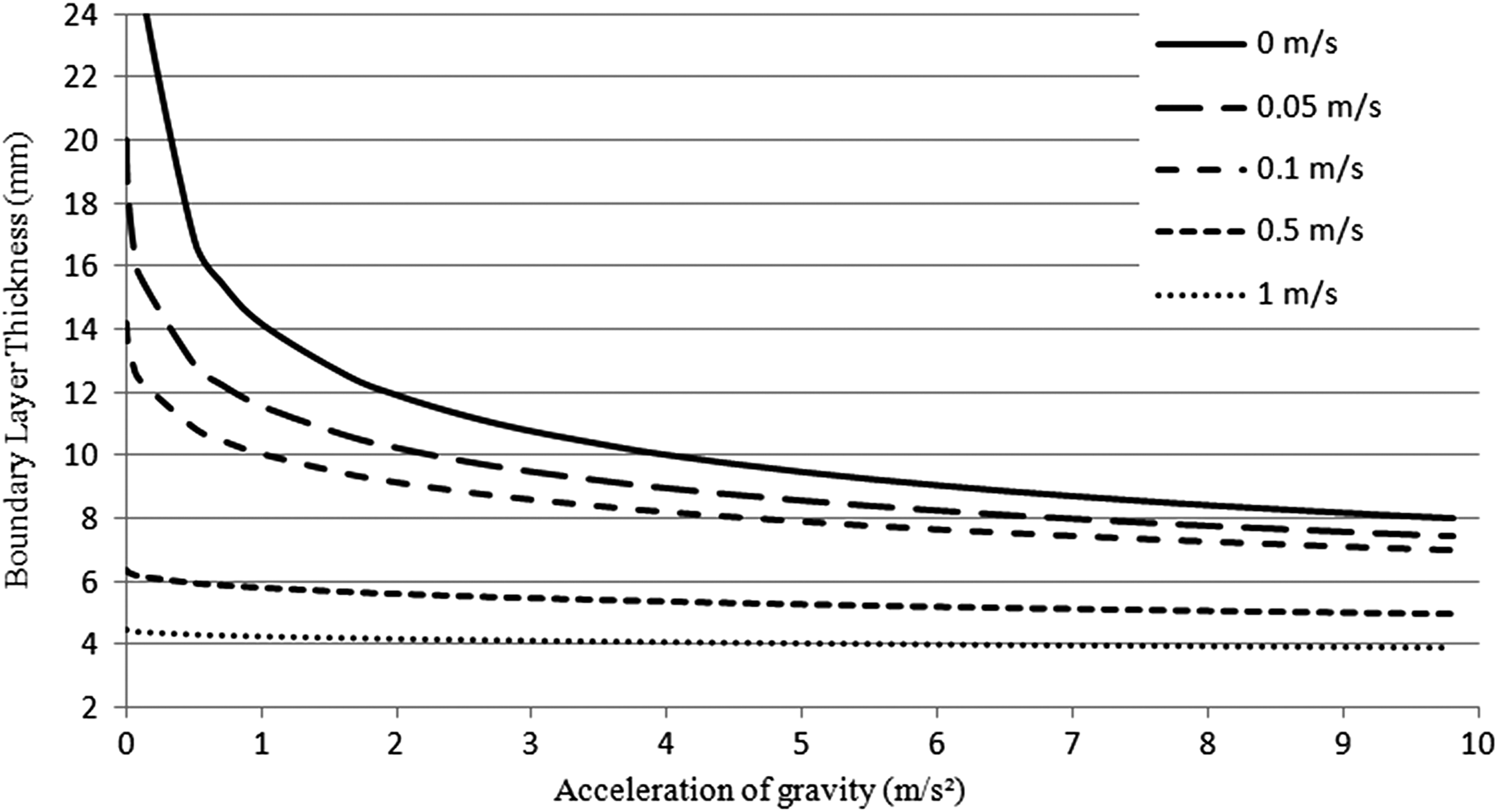
Variations of boundary layer thickness according to the acceleration of gravity between 0.000001 and 9.807 m·s⁻² for five different forced convection velocities: 0 m·s⁻¹ (plain); 0.05 m·s⁻¹ (long dashes); 0.1 m·s⁻¹ (dashes); 0.5 m·s⁻¹ (small dashes); and 1 m·s⁻¹ (dots).

The higher the value of g and of forced convection, the lower the boundary layer. In lunar gravity (1.625 m·s⁻²) with no forced convection, the boundary layer is 50% thicker than in Earth gravity conditions and 20% thicker than in martian gravity (3.711 m·s⁻²). It is interesting to note that in Earth's gravity, the boundary layer is twice as thick with no forced convection compared with a forced convection of 1 m·s⁻¹, while it is 10 times thicker in microgravity.

3.2. Mass exchange rates versus gravity and forced convection

The previous boundary layer model is now used for assessing rates of mass exchanges between the gas bulk and the leaf surface. The water transpiration and CO₂ uptake rates per surface of leaf area were computed for values of g varying from 0.000001 m·s⁻² (microgravity) to 9.807 m·s⁻² (Earth's gravity) and for five different forced convection velocities, from 0 to 1 m·s⁻¹.

As expected, the transpiration and CO₂ uptake rates are higher for higher forced convection velocities and higher gravity levels. Both CO₂ uptake and transpiration rates in Earth gravity conditions are twice as high for a forced convection of 1 m·s⁻¹ compared with no forced convection; they are, respectively, 2.5 and 2.3 times higher in martian gravity and both almost three times higher in lunar gravity (Fig. 4).

FIG. 4.

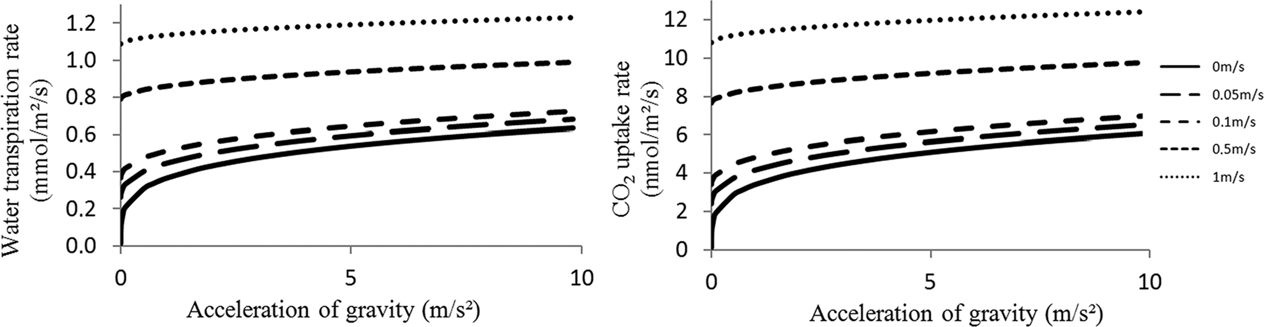
Variations of the water transpiration rate (left) and the CO₂ uptake rate (right) according to acceleration of gravity between 0.000001 and 9.807 m·s⁻² for five different forced convection velocities: 0 m·s⁻¹ (plain); 0.05 m·s⁻¹ (long dashes); 0.1 m·s⁻¹ (dashes); 0.5 m·s⁻¹ (small dashes); and 1 m·s⁻¹ (dots).

3.3. Biomass production versus gravity and forced convection

By using equations of the model described in the work of Hézard (2012) and Poulet et al. (2017), the biomass fresh weight of a lettuce crop was computed over a growth period of 50 days and under 400 μmol·m⁻²·s⁻¹ of incident light for three different gravity levels (microgravity, martian, and Earth) and three forced convection velocities (Fig. 5). It is to be underlined that in Earth's gravity after 50 days, biomass production is three times as much with a forced convection of 1 m·s⁻¹ compared with no forced convection and 50% higher with a forced convection of 0.5 m·s⁻¹.

FIG. 5.

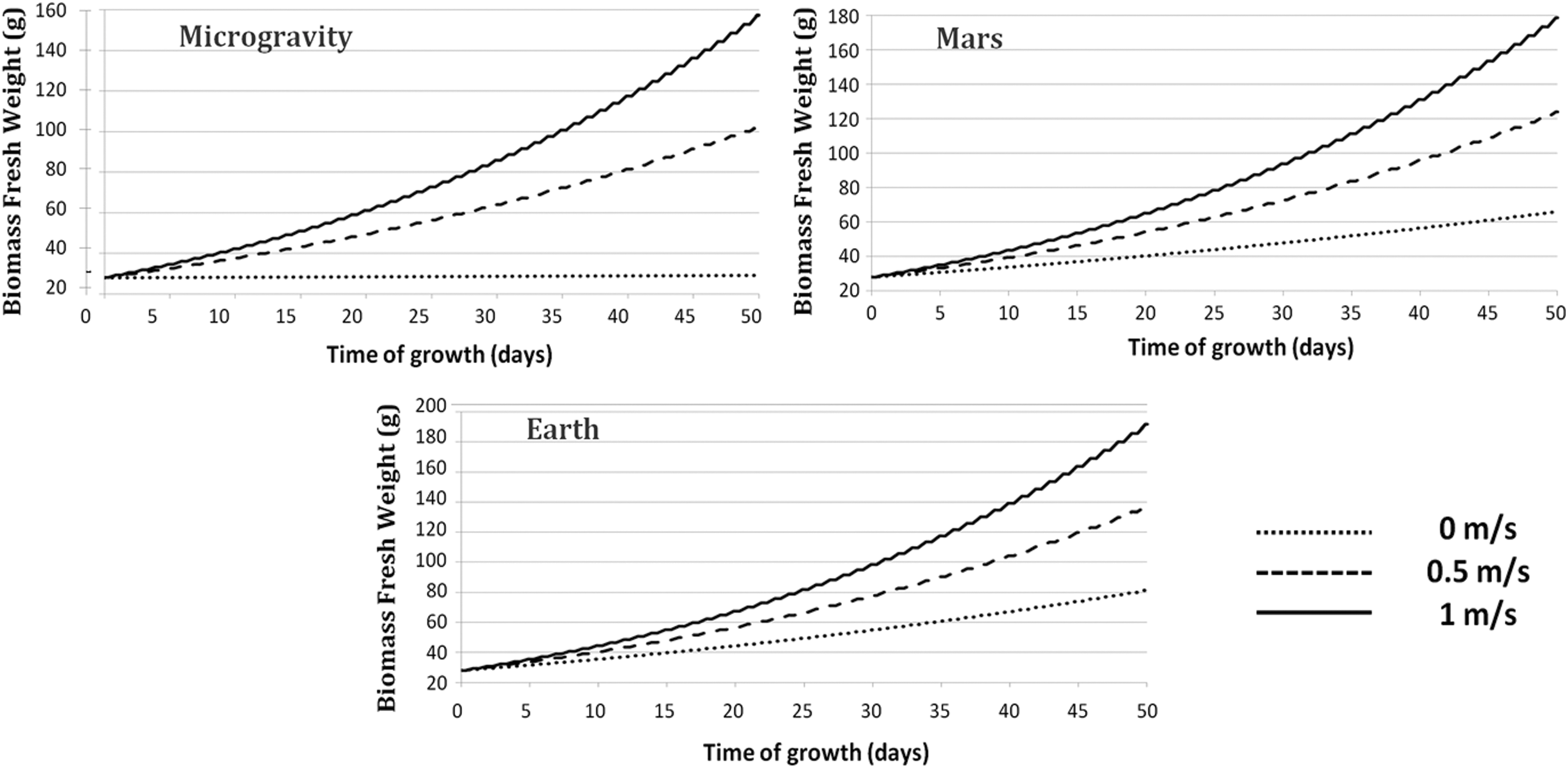
Biomass fresh weight accumulation over time in microgravity (top left), in martian gravity (top right), and in Earth's gravity (bottom) for three different forced convection velocities: 0 m·s⁻¹ (dotted line); 0.5 m·s⁻¹ (dashed line); and 1 m·s⁻¹ (plain line).

With no forced convection, biomass production is 25% higher in Earth gravity conditions than in martian gravity conditions and it is a little >1 g in microgravity. With a forced convection of 0.5 m·s⁻¹, biomass production is over 20% higher in martian gravity conditions than in microgravity and 40% higher in Earth gravity conditions.

4. Discussion

4.1. Boundary layer thickness

The thickness of the boundary layer is more sensitive to gravity for lower values of forced convection. Indeed, with the parameters of the model, the value of free convection velocity varies between 0.001 m·s⁻¹ in microgravity and 0.31 m·s⁻¹ in Earth's gravity. Hence, for values of forced convection >0.3 m·s⁻¹, the forced convection term prevails over the free convection term. This highlights the existence of a threshold value for forced convection velocity, under which boundary layer thickness depends on gravity levels and above which it mainly depends on forced convection. This threshold value gives the range of the mixed convection domain where free and forced convection effects are of the same order of magnitude: Ri ∼1.

This boundary layer model is valid for a single leaf with a circular shape, exchanging gas only from the upper side of the leaf. The results for a whole plant will be slightly different since the shape of the plant is more complex, inducing aerodynamic interference between leaves such as eddy shedding and flow channeling (Schuepp, 1993), and since air velocity on the top and bottom of the plant is different. When this model is extrapolated to a whole canopy, the significant boundary layer will be that of the canopy, which is characterized with a shelter factor (Schuepp, 1993) and is more complex than a simple addition of the boundary layers of each individual plant.

4.2. Gas exchanges and biomass production

As noticed in the case of the boundary layer thickness, the gas exchange rates are more sensitive to the influence of gravity for lower forced convection velocities, and there is a threshold value under which water transpiration and CO₂ uptake depend on gravity levels and above which they depend on the forced convection velocity value. It would be interesting to simulate gas exchanges for a whole plant and then for a whole canopy to investigate if this threshold value holds at a larger scale. If it does, it means that in future greenhouse modules for food production, it will be crucial to ensure an adequate ventilation level around each plant to ensure optimum gas exchanges everywhere.

The results on biomass production underline the fact that it will be different on other celestial bodies, during planetary travels, and in the Earth's orbit than on Earth's surface; it also shows that adjusting the ventilation to an adequate level can lead to biomass production levels similar to those achieved in Earth gravity conditions. It is thus necessary to study the intricate relationship between forced convection, gravity levels, and biomass production to predict how much food can be produced during long-duration space missions.

Conclusion

This study highlights the importance of understanding interactions of gravity and convection on the leaf boundary layer to reliably predict biomass production, water recycling, and air revitalization in space conditions. The next step will include an energy balance and focus on variations of leaf temperature with gravity and convection. These results will be validated by experimental data with a parabolic flight experiment and ultimately it will lead to a thorough and accurate mechanistic model of plant growth in reduced gravity environments, including mass and energy balances.

Footnotes

Acknowledgments

The authors thank the Centre National d'Etudes Spatiales (CNES) and the Centre National de la Recherche Scientifique (CNRS) for financially supporting this work, the Institut Pascal for providing their facilities, and the ESA MELiSSA project for the support, as well as Dr. Jérôme Ngao and Dr. Marc Saudreau from the Institut National de Recherche Agronomique (INRA) for their fruitful discussions.

Author Disclosure Statement

No competing financial interests exist.

Abbreviations Used

References

Anderson

M.S.

, Ewert

M.K.

, Keener

J.F.

, and Wagner

S.A.

(2015) Life Support Baseline Values and Assumptions Document, NASA/TP-2015–218570. NASA Johnson Space Center, Houston, TX.

Beek

W.J.

, Muttzall

K.M.K.

, and van Heuven

J.W.

(1999) Transport Phenomena, 2nd ed. Wiley, Chichester and New York.

Boulard

, Mermier

, Fargues

, Smits

, Rougier

, and Roy

J.C.

(2002) Tomato leaf boundary layer climate: implications for microbiological whitefly control in greenhouses. Agric For Meteorol, 110:159–176.

Clauwaert

, Ilgrande

, Christiaens

, Lindeboom

, Luther

, Muys

, Alloul

, Dussap

C.-G.

, Godia

, Sas

, Boon

, Rabaey

, Leys

, Geelen

, and Vlaeminck

(2015) The nitrogen cycle in life support systems. In: COSPAR, 2nd Symposium, Abstracts. Presented at the 2nd COSPAR symposium: Water and life in the universe.

Dong

, Fu

, Xie

, Wang

, and Liu

(2017) Element cycling and energy flux responses in ecosystem simulations conducted at the Chinese Lunar Palace-1. Astrobiology, 17:78–86.

Drayer

G.E.

and Howard

A.M.

(2014) Modeling and simulation of an aquatic habitat for bioregenerative life support research. Acta Astronaut, 93:138–147.

Eckart

(1996) Spaceflight Life Support and Biospherics. Microcosm Press, Netherlands.

Ehleringer

and Björkman

(1977) Quantum yields for CO₂ uptake in C3 and C4 plants: dependence on temperature, CO₂, and O₂ concentration. Plant Physiol, 59:86–90.

Ewert

M.K.

, Drysdale

A.E.

, Levri

J.A.

, Duffield

B.E.

, Hanford

A.J.

, Lange

K.E.

, and Stafford

K.W.

(2002) Advanced Life Support Requirements, Assumptions and Reference Missions (SAE Technical Paper No. 2002-01-2480). SAE Technical Paper, Warrendale, PA.

10.

, Li

, Xie

, Dong

, Wang

, Jia

, Shao

, Dong

, Deng

, Liu

Hui

, Liu

, Hu

, and Liu, Hong. (2016) How to establish a bioregenerative life support system for long-term crewed missions to the Moon or Mars. Astrobiology, 16:925–936.

11.

Furfaro

, Sadler

, and Giacomelli

(2016) Mars-lunar greenhouse (M-LGH) prototype for bioregenerative life support systems in future planetary outposts. In Proceedings of the International Astronautical Congress, IAC.

12.

Hendrickx

, De Wever

, Hermans

, Mastroleo

, Morin

, Wilmotte

, Janssen

, and Mergeay

(2006) Microbial ecology of the closed artificial ecosystem MELiSSA (Micro-Ecological Life Support System Alternative): reinventing and compartmentalizing the Earth's food and oxygen regeneration system for long-haul space exploration missions. Res Microbiol, 157:77–86.

13.

Hézard

(2012) Higher Plant Growth Modelling for Life Support Systems: Global Model Design and Simulation of Mass and Energy Transfers at the Plant Level. PhD thesis, Doctoral School of Life Sciences, Health, Agronomy, Environment. Université Blaise Pascal, Université d'Auvergne, Clermont-Ferrand.

14.

Hézard

, Sasidharan

, Cruely

, and Dussap

C.-G.

(2010) Higher plants modeling for bioregenerative life support applications: general structure of modeling. In 40th International Conference on Environmental Systems (ICES). American Institute of Aeronautics and Astronautics.

15.

Hirai

and Kitaya

(2009) Effects of gravity on transpiration of plant leaves. Ann N Y Acad Sci, 1161:166–172.

16.

Holmberg

, Paille

, and Lasseur

(2013) Preliminary modelling of mass flux at the surface of plant leaves within the MELiSSA higher plant compartments. Master's thesis, Uppsala University, ESA.

17.

Jones

H.G.

and Rotenberg

(2001) Energy, radiation and temperature regulation in plants. eLS. doi:10.1002/9780470015902.a0003199.pub2.

18.

Kitaya

. (2016) Air current around single leaves and plant canopies and its effect on transpiration, photosynthesis, and plant organ temperatures. In LED Lighting for Urban Agriculture, edited by Kozai

, Fujiwara

, and Runkle

E.S.

, Springer, Singapore, pp 177–187.

19.

Kitaya

, Tsuruyama

, Kawai

, Shibuya

, and Kiyota

(2000) Effects of air current on transpiration and net photosynthetic rates of plants in a closed plant production system. In Transplant Production in the 21st Century, edited by C. Kubota and C. Chun, Springer, Netherlands, pp 83–90.

20.

Kitaya

, Kawai

, Tsuruyama

, Takahashi

, Tani

, Goto

, Saito

, and Kiyota

(2001) The effect of gravity on surface temperature and net photosynthetic rate of plant leaves. Adv Space Res, 28:659–664.

21.

Kitaya

, Kawai

, Tsuruyama

, Takahashi

, Tani

, Goto

, Saito

, and Kiyota

(2003a) The effect of gravity on surface temperatures of plant leaves. Plant Cell Environ, 26:497–503.

22.

Kitaya

, Tsuruyama

, Shibuya

, Yoshida

, and Kiyota

(2003b) Effects of air current speed on gas exchange in plant leaves and plant canopies. Adv Space Res, 31:177–182.

23.

Kitaya

, Shibuya

, Yoshida

, and Kiyota

(2004) Effects of air velocity on photosynthesis of plant canopies under elevated CO₂ levels in a plant culture system. Adv Space Res, 34:1466–1469.

24.

Lambers

, Chapin

F.S.

, and Pons

T.L.

(2008) Plant Physiological Ecology, 2nd ed. Springer, New York.

25.

Lasseur

, Brunet

, de Weever

, Dixon

, Dussap

, Godia

, Leys

, Mergeay

, and Van Der Straeten

(2011) MELiSSA: the European project of closed life support system. Grav Space Res, 23:3–12.

26.

Mitchell

C.A.

(1994) Bioregenerative life-support systems. Am J Clin Nutr, 60:820S–824S.

27.

Monje

, Bingham

G.E.

, Carman

J.G.

, Campbell

W.F.

, Salisbury

F.B.

, Eames

B.K.

, Sytchev

, Levinskikh

M.A.

, and Podolsky

(2000) Canopy photosynthesis and transpiration in micro-gravity: gas exchange measurements aboard Mir. Adv Space Res, 26:303–306.

28.

Monje

, Stutte

, and Chapman

(2005) Microgravity does not alter plant stand gas exchange of wheat at moderate light levels and saturating CO₂ concentration. Planta, 222:336–345.

29.

Muchow

R.C.

and Sinclair

T.R.

(1989) Epidermal conductance, stomatal density and stomatal size among genotypes of Sorghum bicolor (L.) Moench. Plant Cell Environ, 12:425–431.

30.

Poulet

, Fontaine

J.-P.

, and Dussap

C.-G.

(2016) Plant's response to space environment: a comprehensive review including mechanistic modelling for future space gardeners. Bot Lett, 163:337–347.

31.

Poulet

, Dussap

C.-G.

, and Fontaine

J.-P.

(2017) Modelling higher plants gas exchange in reduced gravity environment. Presented at the 47th International Conference on Environmental Systems (ICES). July 16–20, 2017. Charleston, SC.

32.

Raschke

(1960) Heat transfer between the plant and the environment. Annu Rev Plant Physiol, 11:111–126.

33.

Schuepp

P.H.

(1993) Tansley review no. 59 leaf boundary layers. New Phytol , 125:477–507.

34.

Schymanski

S.J.

, Or

, and Zwieniecki

(2013) Stomatal control and leaf thermal and hydraulic capacitances under rapid environmental fluctuations. PLoS One, 8:e54231.

35.

Siegel

and Howell, J.R. (1992) Thermal Radiation and Heat Transfer, 3rd ed. Hemisphere, New York, 1992.

36.

Vesala

(1998) On the concept of leaf boundary layer resistance for forced convection. J Theor Biol, 194:91–100.

37.

Wheeler

R.M.

(2003) Carbon balance in bioregenerative life support systems: some effects of system closure, waste management, and crop harvest index. Adv Space Res, 31:169–175.

38.

Wheeler

R.M.

(2004) Horticulture for Mars. Acta Hortic, 642:201–215.

39.

Wheeler

R.M.

(2011) Plants for human life support in space: from Myers to Mars. Grav Space Res, 23:25–35.

40.

Wheeler

R.M.

(2017) Agriculture for space: people and places paving the way. Open Agriculture, 2:14–32.