On the Rate of Abiogenesis from a Bayesian Informatics Perspective

Abstract

Life appears to have emerged relatively quickly on the Earth, a fact sometimes used to justify a high rate of spontaneous abiogenesis (λ) among Earth-like worlds. Conditioned upon a single datum—the time of earliest evidence for life (t _obs)—previous Bayesian formalisms for the posterior distribution of λ have demonstrated how inferences are highly sensitive to the priors. Rather than attempt to infer the true λ posterior, we here compute the relative change to λ when new experimental/observational evidence is introduced. By simulating posterior distributions and resulting entropic information gains, we compare three experimental pressures on λ: (1) evidence for an earlier start to life, t _obs, (2) constraints on spontaneous abiogenesis from the laboratory, and (3) an exoplanet survey for biosignatures. First, we find that experiments 1 and 2 can only yield lower limits on λ, unlike 3. Second, evidence for an earlier start to life can yield negligible information on λ if \documentclass{aastex}\usepackage{amsbsy}\usepackage{amsfonts}\usepackage{amssymb}\usepackage{bm}\usepackage{mathrsfs}\usepackage{pifont}\usepackage{stmaryrd}\usepackage{textcomp}\usepackage{portland, xspace}\usepackage{amsmath, amsxtra}\usepackage{upgreek}\pagestyle{empty}\DeclareMathSizes{10}{9}{7}{6}\begin{document}$${t_{{ \rm{obs}}}} \ll \lambda _{ \max }^{ - 1}$$ \end{document} . Vice versa, experiment 2 is uninformative when \documentclass{aastex}\usepackage{amsbsy}\usepackage{amsfonts}\usepackage{amssymb}\usepackage{bm}\usepackage{mathrsfs}\usepackage{pifont}\usepackage{stmaryrd}\usepackage{textcomp}\usepackage{portland, xspace}\usepackage{amsmath, amsxtra}\usepackage{upgreek}\pagestyle{empty}\DeclareMathSizes{10}{9}{7}{6}\begin{document}$${ \lambda _{{ \rm{max}}}} \gg t_{{ \rm{obs}}}^{ - 1}$$ \end{document} . While experiment 3 appears the most direct means of measuring λ, we highlight that early starts inform us of the conditions of abiogenesis and that laboratory experiments could succeed in building new life. Altogether, the three experiments are complementary, and we encourage activity in all to solve this grand challenge.

1. Introduction

The number of communicative civilizations in our galaxy is often framed in terms of the famous Drake equation, described by seven parameters which can be considered to guide the observational inputs needed to make an inference. When first proposed by Drake (1965) over a half a century ago, all the terms were essentially unknown, but today, observational constraints exist for the first three terms: the rate of star formation (Robitaille and Whitney, 2010), the fraction of stars with planets (Cassan et al., 2012), and the average number of habitable planets per star (Foreman-Mackey et al., 2014; Dressing and Charbonneau, 2015). It is therefore timely to consider what type of observations might enable us to best constrain the next term, f_l , the fraction of habitable planets which develop life.

At the time of writing, interstellar panspermia is considered to be an unlikely pathway for planets to develop life (Wessen, 2010), which leaves the most likely pathway as being abiogenesis: the spontaneous process by which inert matter becomes living.

The rate of abiogenesis, λ, is surely functionally dependent on the very specific geophysical, chemical, and environmental conditions of a given world (Scharf and Cronin, 2016). For example, it would seem manifestly wrong to assume that frigid Pluto should have the same rate of abiogenesis events as the early Earth. Consequently, one might reasonably ask whether knowledge of the Earth's rate of abiogenesis has any useful merit for predicting the prevalence of life elsewhere. While this is certainly a reasonable and valid concern, we are frankly left with no choice but to operate under the assumption that the Earth and Earth-like exoplanets belong to the same distribution.

This concern can at least be somewhat mitigated against by assuming that the Earth's rate of abiogenesis is a representative sample drawn for a particular subset of planet types, namely “Earth-like” planets. The precise definition of what constitutes a member of this subset is an in-depth discussion in of itself (Tasker et al., 2017), but let us continue under the assumption that such a definition can be expressed, whatever it may be.

There are no other known examples of life beyond the Earth. Furthermore, all known extant and extinct forms of life are generally thought to share a universal common ancestor, an idea which was first suggested by Darwin (1859) and today forms a central pillar of modern evolutionary theory (Sober, 2008). We are therefore faced with the challenge of trying to infer the rate of abiogenesis from a single datum. Furthermore, we cannot exclude the possibility that multiple abiogenesis events occurred or are indeed in the process of occurring, merely that at least one event transpired, which led to a planet-dominating tree of life. A statistic of one is difficult to work with at the best of times, but the situation is exacerbated by the anthropic bias that we would not be here had at least one event not been successful.

A critical piece of observational evidence guiding these discussions is that life appears to have emerged on the Earth over 3.5 billion years ago (Schopf et al., 2007) and thus relatively early. From this observation, there have been numerous efforts to quantify λ conditioned upon this datum, with, for example, Carter (1983) concluding that it is compatible with life being rare, whereas the findings of Lineweaver and Davis (2002) point strongly toward life being common on Earth-like worlds.

A significant advancement in the statistical treatment was presented in the study of Spiegel and Turner (2012), who cast the problem in a Bayesian framework. As we show later in a rederivation of their formalism, this naturally accounts for the selection bias imposed by the fact that our existence is conditioned upon a success. A key conclusion of Spiegel and Turner (2012) was that the probability distribution of λ conditioned upon the observation of life's early emergence, known as the posterior, is highly sensitive to what prior assumptions (including tacit assumptions) impose about how λ is distributed, known as the prior.

In general, the functional form and corresponding shape parameters describing the prior probability distribution for λ are completely unknown. Even changing between different but ostensibly reasonable uninformative priors (Lacki, 2016) leads to dramatic changes in the posterior (Spiegel and Turner, 2012), given the current data in hand.

Rather than try to estimate the absolute posterior of λ, which may be simply infeasible with present information, a more achievable goal is to compare how the posterior would be expected to change if additional information was obtained—a distinct approach. By quantifying how much we learn from various hypothetical experiments, the goal here is to guide future experimenters as to which strategies are most likely to constrain λ, and critically in what way does each experiment constrain it. Accordingly, in this work, we consider three types of experiments that might be expected to constrain λ:

An earlier estimate for the time at which life first appeared on the Earth, t _obs.

An upper limit on the rate of abiogenesis, λ _max [e.g., from a series of Miller and Urey (1959) type laboratory experiments].

The unambiguous detection or null detection of life among a subset of N Earth-like exoplanets/exomoons.

Observational evidence for an earlier t _obs may come from numerous different sources, but the details are unimportant for this work—we only assume that the evidence is unambiguous. This means that we do not invoke a probabilistic model where the data itself are uncertain since the probability distribution describing that uncertainty would be itself unknown.

In a similar vein, an upper limit on λ from laboratory experiments is not a soft probabilistic threshold but assumed to be a hard cutoff since again the softness shape would add additional unknowns into our model. Furthermore, we do not consider the more informative case of an actual instance of spontaneous laboratory-based abiogenesis in this work. If reproducible, such a detection would be so constraining that it would make the results of our article moot and is therefore not worth including here.

Finally, extraterrestrial examples of life are formally (but not necessarily strictly) limited to extrasolar worlds (i.e., not endoworlds such as Mars) to greatly reduce the false-alarm probability that the observed life is in fact related to us via a prior panspermia event. We also assume that it is possible to collect observations that can categorically determine whether an extrasolar body has or does not have recognizable life. In this way, one might limit our definition of λ to being only applicable to events, which ultimately lead to recognizable life. For example, it is possible that a body is inhabited by a life form which produces almost no biosignatures, making remote detection effectively impossible, and our λ rate would not include these more elusive organisms. A final caveat is that the planets/moons in this sample should be not only Earth-like now but also Earth-like for geological timescales (we formally adopt 5 Gyr as a representative habitable age).

In each of these three experiments, we can compare how the posterior distribution for λ is expected to change, both qualitatively and quantitatively. Before doing so, it is necessary to first formally introduce our Bayesian framework in Section 2. Following this, we describe the results of the three experiments in Section 3. Finally, Section 4 summarizes our findings and describes the main conclusions of this work, as well listing the limitations of this exercise.

2. Bayesian Model

2.1. A uniform rate model for abiogenesis

We follow the prescription of Spiegel and Turner (2012) in adopting the simple yet reasonable assumption that abiogenesis events occur at a uniform rate over time, thus following a Poisson process. Let us denote the Poisson shape parameter as λ, which describes the mean number of abiogenesis events, N, occurring in a fixed time interval, which we set to a Gyr. For example, a rate of λ = 4 means that, on average, four abiogenesis events occur every Gyr. The probability distribution for the number of events that actually occur is described by a Poisson distribution, with a shape parameter λ, that is, N∼Poisson(λ). Over a time interval of t then, the expectation value for the number of abiogenesis events would be λt. Consequently, the probability of N abiogenesis events having transpired during a time interval t is \documentclass{aastex}\usepackage{amsbsy}\usepackage{amsfonts}\usepackage{amssymb}\usepackage{bm}\usepackage{mathrsfs}\usepackage{pifont}\usepackage{stmaryrd}\usepackage{textcomp}\usepackage{portland, xspace}\usepackage{amsmath, amsxtra}\usepackage{upgreek}\pagestyle{empty}\DeclareMathSizes{10}{9}{7}{6}\begin{document} \begin{align*} \Pr ( N \vert \lambda , t ) = { e^ { - \lambda t } } { \frac { { { ( \lambda t ) } ^N } } { N! } } . \tag { 1 } \end{align*} \end{document}

2.2. Time for life to emerge as an exponential distribution

As discussed in Section 1, we do not know how many abiogenesis events have occurred on the Earth to date, only that at least one must have occurred over a time interval t, where t represents the interval from now back to when the Earth first became capable of supporting life. The probability of at least one abiogenesis event occurring in this time is unity minus the probability of zero events occurring, or equivalently, the probability of life emerging on a planet within a time t is \documentclass{aastex}\usepackage{amsbsy}\usepackage{amsfonts}\usepackage{amssymb}\usepackage{bm}\usepackage{mathrsfs}\usepackage{pifont}\usepackage{stmaryrd}\usepackage{textcomp}\usepackage{portland, xspace}\usepackage{amsmath, amsxtra}\usepackage{upgreek}\pagestyle{empty}\DeclareMathSizes{10}{9}{7}{6}\begin{document} \begin{align*} \begin{split} \Pr ( N \ge 1 \vert \lambda , t ) & = 1 - \Pr ( N = 0 \vert \lambda , t ) , \\ & = 1 - {e^{ - \lambda t}} , \\\end{split} \tag{2}\end{align*} \end{document}

which is the cumulative density function (CDF) of an exponential distribution. When we consider that this CDF describes the probability that life arose by a time t, it therefore follows that the probability distribution for the time at which life first arose, which we can denote as t _life, must be an exponential distribution, that is, t _life ∼ Ɛ (λ).

2.3. Accounting for selection bias

For the moment, let us treat t _life as a random variable drawn from Ɛ (λ) with no other constraints whatsoever on its value (i.e., we have not yet included the paleontological information regarding the earliest evidence for life). Consider setting λ to be some low rate, such as 0.01 Gyr⁻¹. In such a case, the vast majority of random draws from the probability distribution describing t _life will exceed ∼4.5 Gyr. Even if the Earth can be considered to be habitable immediately after the hypothesized Moon-forming impact 4.47 Gyr ago (Bottke et al., 2015), clearly, draws exceeding this age are incompatible with humanity's existence, else life should not have arisen yet. Accordingly, one might justifiably include this constraint into our statistical treatment by setting the maximum limit on t _life to be less than 4.5 Gyr.

More generally, one might reasonably argue that 4.5 Gyr is too optimistic and that following the Moon-forming impact, it would have taken some time for conditions to be suitable for life—for example, a crust likely did not condense until 4.4 Gyr ago (Valley et al., 2014). However, one might argue that even if conditions were immediately suitable for life, 4.5 Gyr is still too generous a maximum limit, since had life begun just 0.5 Gyr ago, there would have been insufficient time for intelligent observers, such as ourselves, to have evolved. We may absorb these arguments into a single term, τ, which describes the latest time for which life could have arisen on the Earth and yet still be compatible with both the habitable history of our planet and the time it would take intelligent observers such as ourselves to evolve. The selection bias introduced by τ can be formally encoded into our model by applying a truncation to the probability density function (PDF) for t _life, such that \documentclass{aastex}\usepackage{amsbsy}\usepackage{amsfonts}\usepackage{amssymb}\usepackage{bm}\usepackage{mathrsfs}\usepackage{pifont}\usepackage{stmaryrd}\usepackage{textcomp}\usepackage{portland, xspace}\usepackage{amsmath, amsxtra}\usepackage{upgreek}\pagestyle{empty}\DeclareMathSizes{10}{9}{7}{6}\begin{document} \begin{align*} \Pr ( { t_ { { \rm { life } } } } ;\ \tau ) = { \frac { \lambda { e^ { - \lambda { t_ { { \rm { life } } } } } } } { 1 - { e^ { - \lambda \tau } } } } . \tag { 3 } \end{align*} \end{document}

2.4. Accounting for observation time

Consider that we have some measurements for the existence of the earliest life on the Earth, which occurs at a time t = t _obs. We set t = 0 to be the time at which the planet became habitable, and thus, t _obs is perhaps better thought of as the difference between these two times. We set the reference time this way to remove a degree of freedom from our model, in contrast to Spiegel and Turner (2012) who left this in as an extra unknown. With our reference time, τ is directly interpreted as the minimum time it takes for life to evolve from whatever biological entity emerged from the abiogenesis event to an intelligent observer.

The measurement of t _obs is our most constraining datum, but the emergence of life must in fact predate this time, such that t _life ≤ t _obs. This constraint can be encoded in our probability framework by evaluating the probability of life emerging before a time t _obs: \documentclass{aastex}\usepackage{amsbsy}\usepackage{amsfonts}\usepackage{amssymb}\usepackage{bm}\usepackage{mathrsfs}\usepackage{pifont}\usepackage{stmaryrd}\usepackage{textcomp}\usepackage{portland, xspace}\usepackage{amsmath, amsxtra}\usepackage{upgreek}\pagestyle{empty}\DeclareMathSizes{10}{9}{7}{6}\begin{document} \[\Pr ({t_{{\text{life}}}} \leqslant {t_{{\text{obs}}}};\;\tau ) = \int_{{t_{{\text{life}}}} = 0}^{{t_{{\text{life = }}{t_{{\text{obs}}}}}}} {\frac{{\lambda {e^{ - \lambda {t_{{\text{life}}}}}}}}{{1 - {e^ - }^{\lambda \tau }}}{\text{d}}{t_{{\text{life}}}},} {\text{ }} \tag { 4 }\] \end{document}

which, after simplification, gives \documentclass{aastex}\usepackage{amsbsy}\usepackage{amsfonts}\usepackage{amssymb}\usepackage{bm}\usepackage{mathrsfs}\usepackage{pifont}\usepackage{stmaryrd}\usepackage{textcomp}\usepackage{portland, xspace}\usepackage{amsmath, amsxtra}\usepackage{upgreek}\pagestyle{empty}\DeclareMathSizes{10}{9}{7}{6}\begin{document} \begin{align*} \Pr ( { t_ { { \rm { life } } } } \le { t_ { { \rm { obs } } } } ;\ \tau ) = { \frac { 1 - { e^ { - \lambda { t_ { { \rm { obs } } } } } } } { 1 - { e^ { - \lambda \tau } } } } . \tag { 5 } \end{align*} \end{document}

2.5. Likelihood function for λ

Consider that we wanted to infer λ, conditioned upon a measurement of t _obs, in words we wish to infer \documentclass{aastex}\usepackage{amsbsy}\usepackage{amsfonts}\usepackage{amssymb}\usepackage{bm}\usepackage{mathrsfs}\usepackage{pifont}\usepackage{stmaryrd}\usepackage{textcomp}\usepackage{portland, xspace}\usepackage{amsmath, amsxtra}\usepackage{upgreek}\pagestyle{empty}\DeclareMathSizes{10}{9}{7}{6}\begin{document} \[\underbrace {\Pr (\lambda |{t_{{\text{obs}}}})}_{{\text{posterior}}} = \frac{{\overbrace {\Pr ({t_{{\text{obs}}}}|\lambda )}^{{\text{likelihood}}}\overbrace {\Pr (\lambda )}^{{\text{prior}}}}}{{\underbrace {\Pr ({t_{{\text{obs}}}})}_{{\text{evidence}}}}} \tag { 6 }\] \end{document}

The likelihood function is given by Equation 5 or rewriting in a conditional form: \documentclass{aastex}\usepackage{amsbsy}\usepackage{amsfonts}\usepackage{amssymb}\usepackage{bm}\usepackage{mathrsfs}\usepackage{pifont}\usepackage{stmaryrd}\usepackage{textcomp}\usepackage{portland, xspace}\usepackage{amsmath, amsxtra}\usepackage{upgreek}\pagestyle{empty}\DeclareMathSizes{10}{9}{7}{6}\begin{document} \begin{align*} \Pr ( { t_ { { \rm { obs } } } } \vert \lambda ) = { \frac { 1 - { e^ { - \lambda { t_ { { \rm { obs } } } } } } } { 1 - { e^ { - \lambda \tau } } } } , \tag { 7 } \end{align*} \end{document}

which is similar to the result obtained by Spiegel and Turner (2012). This is not surprising given we began from the same basic assumption of a uniform rate model for abiogenesis, but we hope our independent action on the derivation more clearly explains its origins. It is worth noting that the likelihood function has a maximum at λ → ∞ and displays asymptotic behavior toward that limit.

2.6. Multiplanet likelihood function for λ

Thus far, we have presented a Bayesian model for inferring the λ conditioned upon evidence for life on the Earth by a time t _obs. An extension to the above, which was not derived by Spiegel and Turner (2012), is to consider surveying N Earth-like worlds for life and detecting M examples of it.

If we surveyed planets and moons in the Solar System, there is a plausible causal connection between the bodies via panspermia (Wessen, 2010), which would significantly complicate the analysis. Instead, we focus on exoplanets where it can be reasonably assumed that each exoplanetary system is an independent sample. Generally, in what follows, we refer to each exoplanetary system as simply a planet for brevity, but this can include systems of planets and moons. The only condition is that only worlds surveyed belong to a subset of worlds, which share similar properties to the Earth, that is, Earth-like.

One difference to our earlier framework is that each exoplanet will typically have a fairly weak age constraint and an even worse constraint on t _obs. This simplifies our analysis though, since we can approximately assume that all planets in the sample share the same age and life simply arose before that age at any time. We set this fiducial age to be 5 Gyr, comparable to the age of the solar system. We make the further assumption that λ is a common value to all planets surveyed. As discussed in Section 1, an assumption of this type is fundamentally necessary to make further progress but can be considered to be justifiable when the survey sample belongs to a class of Earth-like worlds.

The probability that any one of these planets is observed to be a positive detection is given by Equation 2, p = 1 − e^−λt , that is, the likelihood function defined for the single planet case. For simplicity, we assume that all N exoplanets share the same probability of positive detection in each experiment. For each set of N exoplanets, we draw a λ from its prior and perform N Bernoulli experiments with success probability p. The probability of obtaining M successes from a total of N Bernoulli experiments describes a Binomial distribution, and thus, we may write that \documentclass{aastex}\usepackage{amsbsy}\usepackage{amsfonts}\usepackage{amssymb}\usepackage{bm}\usepackage{mathrsfs}\usepackage{pifont}\usepackage{stmaryrd}\usepackage{textcomp}\usepackage{portland, xspace}\usepackage{amsmath, amsxtra}\usepackage{upgreek}\pagestyle{empty}\DeclareMathSizes{10}{9}{7}{6}\begin{document} \begin{align*} \Pr ( N , p;\ M ) = { ( 1 - p ) ^{N - M}}{p^M} \left( { \begin{matrix} N \\ M \\ \end{matrix} } \right) . \tag{8} \end{align*} \end{document}

In the limit of N = 1 and M = 1, we get back the same result for the single-planet case, as expected: \documentclass{aastex}\usepackage{amsbsy}\usepackage{amsfonts}\usepackage{amssymb}\usepackage{bm}\usepackage{mathrsfs}\usepackage{pifont}\usepackage{stmaryrd}\usepackage{textcomp}\usepackage{portland, xspace}\usepackage{amsmath, amsxtra}\usepackage{upgreek}\pagestyle{empty}\DeclareMathSizes{10}{9}{7}{6}\begin{document} \begin{align*} \mathop { \lim } \limits_{N \to 1} \Pr ( N , p;\ M ) = \left\{ { \begin{matrix} p & {{ \rm{if}}} & {M = 1 , } \\ {1 - p} & {{ \rm{if}}} & {M = 0.} \\ \end{matrix} } \right. \tag{9} \end{align*} \end{document}

2.7. Choosing priors for λ and τ

A key result of Spiegel and Turner (2012) is that changing the prior on λ has a major effect on its posterior. As discussed in Section 1, this makes the goal of an absolute determination of the posterior somewhat unachievable, unless we knew what the correct prior was. However, this work is chiefly concerned with how the posterior changes when new information is acquired, seeking the relative differences between hypothetical posteriors rather than the absolute truth. For this reason, the choice of prior is less crucial than before, and we elect to adopt a simple objective prior in the form of a log uniform distribution because it is always positive, admits a wide range of order of magnitudes, and is noninformative with the maximum entropy (in log space): \documentclass{aastex}\usepackage{amsbsy}\usepackage{amsfonts}\usepackage{amssymb}\usepackage{bm}\usepackage{mathrsfs}\usepackage{pifont}\usepackage{stmaryrd}\usepackage{textcomp}\usepackage{portland, xspace}\usepackage{amsmath, amsxtra}\usepackage{upgreek}\pagestyle{empty}\DeclareMathSizes{10}{9}{7}{6}\begin{document} \begin{align*} \Pr ( \lambda ) = \frac { 1 } { \lambda } \frac { 1 } { { \log { \lambda _ { \max } } - \log { \lambda _ { \min } } } } . \tag { 10 } \end{align*} \end{document}

We highlight that this was one of the candidate priors considered by Spiegel and Turner (2012) too. For λ _min, we fix it at 10⁻³ Gyr⁻¹ in the majority of simulations that follow. In contrast, Spiegel and Turner (2012) considered three different values of 10⁻³ Gyr⁻¹, 10⁻¹¹ Gyr⁻¹, and 10⁻²² Gyr⁻¹, which roughly correspond to life occurring only once per 200 stars, once in our galaxy, and once in the observable Universe (assuming one Earth-like planet per star). We will return to these other choices in later in Section 3. The effect λ _max will be investigated in detail as one of our three hypothetical experiments, and so we also discuss this later.

The final term we require a prior for is τ. The largest allowed value for this term is well defined as being the age of the Earth, 4.5 Gyr. The most conservative estimate for the first life on the Earth is ∼3 Gyr ago as Simpson (2017) suggested a 3 Gyr minimum time for life to evolve from the very basic form to being intelligent as we are, which leads to a lower limit of tau to be 1.5 Gyr. Thus, the least informative prior is a uniform distribution given by \documentclass{aastex}\usepackage{amsbsy}\usepackage{amsfonts}\usepackage{amssymb}\usepackage{bm}\usepackage{mathrsfs}\usepackage{pifont}\usepackage{stmaryrd}\usepackage{textcomp}\usepackage{portland, xspace}\usepackage{amsmath, amsxtra}\usepackage{upgreek}\pagestyle{empty}\DeclareMathSizes{10}{9}{7}{6}\begin{document} \begin{align*}{ \rm{Pr}} ( \tau ) \; = { \rm{ \;U}} \left[ {1.5 , 4.5} \right] , \tag{11} \end{align*} \end{document}

and this is the distribution adopted in what follows.

2.8. Sampling method

From a sampling perspective, our model has relatively compact dimensionality and has only a single data point. In such a case, we are able to use a highly efficient sampling algorithm known as the “bootstrap filter,” which is a class of “particle filter” (Künsch, 2013).

To briefly describe the algorithm, first, N sets of hyperparameters \documentclass{aastex}\usepackage{amsbsy}\usepackage{amsfonts}\usepackage{amssymb}\usepackage{bm}\usepackage{mathrsfs}\usepackage{pifont}\usepackage{stmaryrd}\usepackage{textcomp}\usepackage{portland, xspace}\usepackage{amsmath, amsxtra}\usepackage{upgreek}\pagestyle{empty}\DeclareMathSizes{10}{9}{7}{6}\begin{document}$$( \Theta _H^1 , \Theta _H^2 , \ldots , \Theta _H^N )$$ \end{document} are drawn according to the hyper prior distribution. Then, N sets of local parameters are also drawn, given the hyperparameters \documentclass{aastex}\usepackage{amsbsy}\usepackage{amsfonts}\usepackage{amssymb}\usepackage{bm}\usepackage{mathrsfs}\usepackage{pifont}\usepackage{stmaryrd}\usepackage{textcomp}\usepackage{portland, xspace}\usepackage{amsmath, amsxtra}\usepackage{upgreek}\pagestyle{empty}\DeclareMathSizes{10}{9}{7}{6}\begin{document}$$( \Theta _L^i , i = 1 , \ldots , N )$$ \end{document} . Next, we calculate the likelihood of our data, given the parameters (Lⁱ , i = 1,…, N). Finally, we resample parameters (Θ _H, Θ_L) with their corresponding likelihoods L as weights.

In order for the final sampled parameters to be well spread over the parameter space, the parameter space needs to be well explored in the first step. This indicates that the method would not work for high dimensional problems since the required number of samples would be intractable in such a parameter space. In such cases, other sampling methods like Markov chain Monte Carlo (Metropolis, 1953) would be more suitable. But clearly for a simple model like the one we have, the bootstrap filter sampling method is well suited and highly efficient.

2.9. Using information gain to compare different posteriors

The goal of the article is to compare how the λ posterior changes with different experimental setups. To evaluate the difference in a quantitative way, we choose to use the Kullback–Leibler divergence (KLD), which is also known as relative entropy (Kullback and Leibler, 1951). It quantifies the entropy change in going from probability distribution Q to P, where a result of zero implies no difference, and non-zero (but always positive) values imply a finite difference and is given by \documentclass{aastex}\usepackage{amsbsy}\usepackage{amsfonts}\usepackage{amssymb}\usepackage{bm}\usepackage{mathrsfs}\usepackage{pifont}\usepackage{stmaryrd}\usepackage{textcomp}\usepackage{portland, xspace}\usepackage{amsmath, amsxtra}\usepackage{upgreek}\pagestyle{empty}\DeclareMathSizes{10}{9}{7}{6}\begin{document} \begin{align*}{ \rm { KLD ( } } { P } \vert \vert Q ) = \int { { P } ( x ) \log { \frac { { P } ( x ) } { Q ( x ) } } } \, { \rm { d } } x , \tag { 12 } \end{align*} \end{document}

where the integrand limits cover the complete supported domain of the functions P and Q. We highlight that the popular Kolmogorov–Smirnov test (Kolmogorov, 1933; Smirnov, 1948) and Anderson–Darling test (Anderson and Darling, 1952) are primarily designed to test for when two distributions show significant departures from each other and thus would not be directly applicable here. A test statistic, such as the Kolmogorov–Smirnov distance, could be utilized to quantify differences, although we note that this metric only codifies the maximum difference in the CDF between two distributions and does not fully account for the ensemble of differences occurring across the parameter space. For these reasons, we ultimately concluded that the KLD would be a well-suited tool for quantifying the differences observed in our hypothetical experiments.

Computationally, we need to use the discretized version of the equation to calculate the information gain. For this work, we use an R package entropy with all the KLD calculations. However, as the results of the article show, we should not depend only on a number to tell the difference between two distributions. It is useful within each experiment. But when we update the posterior with different experiments, thus changing the posterior in different ways, a number is not enough to describe the results.

3. Results

3.1. Experiment 1: reducing t _obs

3.1.1. Overview

With our model and objective established, we now describe the results from our hypothetical experiments, starting with reducing t _obs. We therefore consider here, what effect would an earlier estimate for the first life on the Earth have on our knowledge concerning the rate of abiogenesis events, λ?

The earliest undisputed evidence for life on the Earth comes from ∼3465 Myr Archean deposits in the Apex Basalt of Western Australia, containing morphotype units, which are concluded to be microfossils in the study of Schopf et al. (2007). Given that the Earth formed 4.54 ± 0.05 Gyr ago (Dalrymple, 2001), the maximum plausible value we can assign to t _obs would be \documentclass{aastex}\usepackage{amsbsy}\usepackage{amsfonts}\usepackage{amssymb}\usepackage{bm}\usepackage{mathrsfs}\usepackage{pifont}\usepackage{stmaryrd}\usepackage{textcomp}\usepackage{portland, xspace}\usepackage{amsmath, amsxtra}\usepackage{upgreek}\pagestyle{empty}\DeclareMathSizes{10}{9}{7}{6}\begin{document}$$\simeq$$ \end{document} 1 Gyr.

In contrast, the very earliest claim for the first evidence of life extends as far back as 4280 Myr ago (Dodd et al., 2017), from putative fossilized microorganisms in ferruginous sedimentary rocks from the Nuvvuagittuq belt in Quebec, Canada. The study of ancient zircons in Jack Hills, Western Australia, indicates the presence of oceans on the Earth as far back as 4408 ± 8 Myr (Wilde et al., 2001), and so one might argue from these studies that t _obs could be as short as ∼100 Myr.

As evident from the cited literature, this is an active and rapidly developing field, and thus, it is quite likely that further revisions to t _obs may occur in the near future. If the age is revised down by another factor of 10, though, how much does this really teach us about λ? The intuitive temptation is to assign earlier start dates with evidence that life is not fussy and can start quite easily, that is, a high λ (Allwood, 2016). As discussed earlier, this question can be more readily addressed in a Bayesian informatics framework such as that presented here.

To investigate this, we computed the posterior for several thousand different hypothetical values of t _obs log-uniformly spaced between 10⁰ Gyr (corresponding to the modern conservative limit) down to 10⁻³ Gyr (a deliberately highly optimistic choice). In each simulation, we fix λ _min = 10⁻³ Gyr⁻¹, as discussed in Section 2.7, but explore four different candidate values for λ _max of 10⁰ Gyr⁻¹, 10¹ Gyr⁻¹, 10² Gyr⁻¹, and 10³ Gyr⁻¹.

3.1.2. Qualitative impacts on the λ posterior

In the right panel of Figure 1, we present the posterior distributions of λ for all four particular t _obs choices when λ _max = 10² Gyr⁻¹ to illustrate the qualitative differences that arise. Broadly speaking, it can be observed that as t _obs becomes smaller, a higher value of the abiogenesis rate is favored. In all cases, the posterior is a monotonic function consistent with a lower limit constraint on λ rather than a peaked quasi-Gaussian measurement. This immediately reveals that measurements of t _obs alone can only hope to ever place probabilistic lower limits on λ and never produce what might be considered as a direct measurement.

FIG. 1.

The left panel shows information gain calculated by KLD as t _obs gets smaller. The right panel gives the detailed posterior distribution of λ for fixed λ _max of 10² Gyr⁻¹. Lines A, B, C, and D represent t _obs of 10⁰ Gyr, 10⁻¹ Gyr, 10⁻² Gyr, and 10⁻³ Gyr, respectively. KLD, Kullback–Leibler divergence.

When t _obs = 10⁰ Gyr (line A), which corresponds to the conservative limit, the posterior stays almost flat after a rise at around λ = 10⁰ Gyr⁻¹ (i.e., one event per Gyr). This can be understood by the observation that we cannot distinguish between, for example, 10 or 100 events per Gyr, as they are sufficient to have t _obs = 10⁰ Gyr. Accordingly, the posterior largely follows the prior. More generally, one expects an inflection point in the posterior to occur at \documentclass{aastex}\usepackage{amsbsy}\usepackage{amsfonts}\usepackage{amssymb}\usepackage{bm}\usepackage{mathrsfs}\usepackage{pifont}\usepackage{stmaryrd}\usepackage{textcomp}\usepackage{portland, xspace}\usepackage{amsmath, amsxtra}\usepackage{upgreek}\pagestyle{empty}\DeclareMathSizes{10}{9}{7}{6}\begin{document}$$\lambda \simeq { \lambda _{{ \rm{inflection}}}} = t_{{ \rm{obs}}}^{ - 1}{ \rm{Gy}}{{ \rm{r}}^{ - 1}}.$$ \end{document}

As t _obs gets larger, higher rate becomes clearly more favorable. The observed posterior morphologies are also responsive to the fact that we set λ _max at 10² Gyr⁻¹. If say, it is set as high as 10⁵ Gyr⁻¹, we should expect all four lines to reach a plateau (which we indeed verified). Accordingly, one can conclude that the actual posterior distribution is highly sensitive to whatever value one adopts for the prior's upper limit, λ _max, reinforcing the conclusions of Spiegel and Turner (2012).

3.1.3. Quantitative impacts on the λ posterior

The left panel of Figure 1 shows the information gain obtained from revising t _obs down. Specifically, we set Q in Equation 12 to be the posterior distribution of λ when t _obs = 10⁰ Gyr, corresponding to our current observational constraint. We do not use the prior on λ since our “starting point” in terms of current knowledge includes a measurement of t _obs and that should be incorporated in our comparison. Accordingly, P in Equation 12 is now set to be equal to the derived posteriors at other choices of t _obs. As a result of this setup, the information gain between P and Q when t _obs = 1 Gyr is, by definition, zero.

The four lines shown broadly reproduce expectation. The information gain increases, resembling a nonlinear logistic function, as t _obs is revised down. Clearly, the choice of λ _max again has a significant impact and specifically seems to control a saturation limit in the information gain. This is most clearly observed for the curve describing λ _max = 10¹ Gyr⁻¹, where there is negligible information gain once t _obs drops below 10^−1.5 Gyr. Indeed, if λ _max = 10⁰ Gyr⁻¹, even our current conservative limit on t _obs lives on this saturated plateau. In such a circumstance, there is essentially no value in paleontologists continuing to try and revise t _obs further back (if their goal is to constrain λ).

The reason behind the saturation can be explained by careful examination of the right panel plot. In the case of line A, the first abiogenesis event happened at t _obs = 1 Gyr. Since there is an inflection point in the posterior at \documentclass{aastex}\usepackage{amsbsy}\usepackage{amsfonts}\usepackage{amssymb}\usepackage{bm}\usepackage{mathrsfs}\usepackage{pifont}\usepackage{stmaryrd}\usepackage{textcomp}\usepackage{portland, xspace}\usepackage{amsmath, amsxtra}\usepackage{upgreek}\pagestyle{empty}\DeclareMathSizes{10}{9}{7}{6}\begin{document}$${ \lambda _{{ \rm{inflection}}}} = t_{{ \rm{obs}}}^{ - 1} \;{ \rm{Gy}}{{ \rm{r}}^{ - 1}}$$ \end{document} (as established earlier), the posterior experiences a steep rise at around once per Gyr. Likewise, lines B/C/D should rise at around 10¹ Gyr⁻¹, 10² Gyr⁻¹, and 10³ Gyr⁻¹, respectively. However, for the case of line D, since the upper limit is set at λ _max = 10² Gyr⁻¹, much of its morphological changes are truncated. This upper limit constraint forces line D to perform similarly like line C. If we translate that to information gain, we can see that point D does not increase very much from point C, and the whole line will gradually saturate.

3.2. Experiment 2: reducing λ _max

3.2.1. Overview

The second type of experimental pressure we consider on λ is one driven by laboratory-based experiments. In particular, we consider the thought experiment where a large suite of containers are constructed, within each exists a representative environment of an Earth-like planet, and simply count how often does life spontaneously emerge from these containers. This is not meant to be a practical experimental setup but rather a toy example of how one might construct a series of experiments to constrain λ in the laboratory.

In principle, one or more of these experiments might successfully spawn a new form of life. If this result was reproducible and verifiable, it would provide such dramatic insights into abiogenesis that comparing it to the other hypothetical experiments in this work is somewhat of a moot point. Instead, we take the pessimistic angle that the experiments do not successfully produce a single abiogenesis event (which is of course consistent with current experiments). In such a case, one could reasonably infer an upper limit on λ from the null results, and thus, we envisage that these experiments return a single new datum for our setup—λ _max.

It is therefore instructive to compare how obtaining ever tighter limits on λ _max affects the posterior on λ without changing t _obs. To do so, we varied λ _max log-uniformly across the same range as used in Section 3.1, from 10³ Gyr⁻¹ to 10⁰ Gyr⁻¹ but now at a much finer resolution. In each simulation, we derive the resulting λ posterior and repeat the entire exercise for four different choices of t _obs, namely 10⁰ Gyr, 10⁻¹ Gyr, 10⁻² Gyr, and 10⁻³ Gyr. Thus, our parameter range directly mirrors the range considered in Section 3.1. As before, λ _min is fixed to 10⁻³ Gyr⁻¹.

3.2.2. Qualitative impacts on the λ posterior

In the right panel of Figure 2, we show four examples of how the λ posterior changes for different λ _max values, keeping a fixed t _obs = 10⁻² Gyr. It is clear that the main difference between the updated posteriors (lines b, c, d) and the original posterior (histogram/line a) is that the posterior becomes truncated at smaller λ values, corresponding directly to λ _max. As a result, while line “a” shows a plateau, this is eroded by the truncation of the sharper λ _max constraints, for similar reasoning as that discussed in Section 3.1.

FIG. 2.

The left panel shows information gain calculated by KLD as λ _max gets smaller. The right panel gives the detailed posterior distribution of λ for fixed t _obs of 10⁻¹ Gyr. Lines a, b, c, and d represent λ _max of 10³ Gyr⁻¹, 10² Gyr⁻¹, 10¹ Gyr⁻¹, and 10⁰ Gyr⁻¹, respectively.

3.2.3. Quantitative impacts on the λ posterior

The left panel of Figure 2 shows the information gain by varying λ _max from 10³ Gyr⁻¹ to 10⁰ Gyr⁻¹, with each of the four lines showing a different assumed t _obs value. In comparison to Figure 1, the information gains are, in general, higher in this second experiment. This can be understood to be resulting from the truncation effect, which significantly elevates the density of lower λ values to maintain normalization. Both experiments 1 and 2 can be seen to provide merely lower limits on λ, rather than a strong measurement, since they are both ultimately conditioned upon the same datum. Nevertheless, in a quantitative sense, our analysis indicates that there is a greater potential for information gain in experiment 2 within the parameter ranges considered.

This conclusion is re-enforced by the fact that none of our simulations in experiment 2 led to a negligible information gain, whereas this was observed in certain cases for experiment 1. Specifically, once λ _max can be constrained to less than or equal to ∼10⁰–10¹ Gyr⁻¹, there is very little information gain to be had from revising t _obs. In contrast, even the most conservative limit on t _obs = 10⁰ Gyr allows for sizable information gains by revising λ _max. Furthermore, the remote possibility of an outright successful abiogenesis event in the laboratory makes a compelling case that this enterprise is more likely to teach us about abiogenesis than experiment 1.

Although we only show lines spanning up to λ _max = 10³ Gyr⁻¹, it is worthwhile to consider the behavior at more extreme choices. As shown in Figure 2, line “a” saturates, but it is only the line to do so. This is because in this case λ _max (which equals 10³ Gyr) substantially exceeds λ _inflection (which equals 10¹ Gyr), allowing for the saturation behavior to take place. We might therefore hypothesize that if we had chosen a far higher choice of λ _max, say 10¹⁰ Gyr⁻¹, then the posterior would broadly look similar to line “a” except the truncation would occur much later. Accordingly, we might hypothesize that if we compared the information gain from λ _max = 10¹⁰ Gyr⁻¹ to λ _max = 10⁹ Gyr⁻¹, there would be very little information gain (compared to, say, going from 10² Gyr⁻¹ to 10¹ Gyr⁻¹) since in both cases \documentclass{aastex}\usepackage{amsbsy}\usepackage{amsfonts}\usepackage{amssymb}\usepackage{bm}\usepackage{mathrsfs}\usepackage{pifont}\usepackage{stmaryrd}\usepackage{textcomp}\usepackage{portland, xspace}\usepackage{amsmath, amsxtra}\usepackage{upgreek}\pagestyle{empty}\DeclareMathSizes{10}{9}{7}{6}\begin{document}$${ \lambda _{{ \rm{max}}}} \gg {\lambda _{{ \rm{inflection}}}}$$ \end{document} . If true, this would mean that if we extended the left panel plot in Figure 2 far to the left (i.e., much higher λ _max), the curves would be very flat until we start to encroach upon values in the domain of λ _inflection. To verify this hypothesis, we repeated the experiments up to λ _max = 10¹⁰ Gyr⁻¹ and indeed verified that the information gain curves are approximately flat when \documentclass{aastex}\usepackage{amsbsy}\usepackage{amsfonts}\usepackage{amssymb}\usepackage{bm}\usepackage{mathrsfs}\usepackage{pifont}\usepackage{stmaryrd}\usepackage{textcomp}\usepackage{portland, xspace}\usepackage{amsmath, amsxtra}\usepackage{upgreek}\pagestyle{empty}\DeclareMathSizes{10}{9}{7}{6}\begin{document}$${ \lambda _{{ \rm{max}}}} \gg {\lambda _{{ \rm{inflection}}}}$$ \end{document} .

3.3. Future evidence from exoplanets

3.3.1. Overview

The third experiment we consider is a future astronomical telescope capable of discerning unambiguously whether an observed exoplanet hosts life or not. As with the previous experiments, the specific details of how this is achieved is not important for the following discussion, although a plausible strategy would be to seek atmospheric biosignatures (Léger et al., 1996). We note surveying a large number of Earth-like worlds is beyond the abilities of existing facilities (Seager, 2014), but it is not unreasonable to suppose that it should be plausible in the future (Rauscher et al., 2015). If the goal of such an enterprise is to quantify our uniqueness and thus the rate at which life springs forth on Earth-like worlds, then the thought experiment described here provides a direct evaluation of how informative such an effort should be expected to be.

Naturally, before having conducted this experiment in reality, the number of abiogenesis detections, M, among a sample N exoplanets is unknown, yet the ratio M/N will clearly strongly affect the resulting λ posterior. To account for this, we therefore have two control variables in this experiment, rather than one: the success rate, M/N, and the survey size, N.

3.3.2. Yield expectations

It is instructive to first pose the question, what kind of ratio value do we actually expect based on current information? A ratio which agrees with our naive expectation (whatever that may be) would lead to only a small change in the λ posterior and thus a small degree of information gain. In contrast, a ratio M/N resulting from this hypothetical survey that in is tension with our prior expectation would dramatically change the λ posterior and thus lead to a large information gain. These considerations provide some initial insight as to why particular values of M/N may not necessarily lead to significant gains in our knowledge of λ. It is therefore interesting and somewhat counterintuitive to note that a survey of N exoplanets for life may not necessarily lead to any substantial gains in our knowledge about the rate of abiogenesis, depending on what ratio of success is observed.

From the above arguments, it is clear that an observed M/N close to our prior expectation on M/N should represent a minimum in the possible information gain. But what exactly is our prior expectation on M/N? Optimists would say life starts everywhere and thus we expect M/N ∼ 1 (Lineweaver and Davis, 2002). If so, then detecting a high success rate in an exoplanet survey would actually teach us very little. Like dropping a coin and seeing it fall to the ground under gravity, results that match expectation generally do not teach us as much as if the coin had travelled upwards. In contrast, a pessimistic might say they are convinced life is rare, and thus, any detection elsewhere would be highly surprising, much like the coin travelling upwards, thereby teaching us a great deal.

We now turn to estimating what our a priori expected M/N should be. This is of course closely related to our current posterior for λ. However, as we have argued earlier and indeed as concluded by Spiegel and Turner (2012), an absolute inference of λ is not possible unless we know what the correct prior should be. Although we have investigated the effect of varying λ _max and this may be constrainable via experiment (Section 3.2), it is unclear how one should assign λ _min at this time (of course another choice is the shape of the prior itself, but we leave that aside at this time).

Using the fiducial choice of λ _min = 10⁻³ Gyr⁻¹, which has been used in both Sections 3.1 and 3.2, our expectation is that M/N is generally quite high. We demonstrate this in the left panel of Figure 3, where we compute the average number of detections expected using our earlier λ posteriors on 5 Gyr old Earth-like planets (by Monte Carlo experiments drawing Bernoulli trials using the probability defined in Equation 2). For almost any choice of t _obs or λ _max (within the ranges used throughout this article), one can observe that M/N is expected to be high. Accordingly, if we set λ _min = 10⁻³ Gyr⁻¹ as before, experiments where we set M/N ∼ 1 will tend to yield minimal gains in information content on λ. We highlight this point carefully due its somewhat counterintuitive consequences.

FIG. 3.

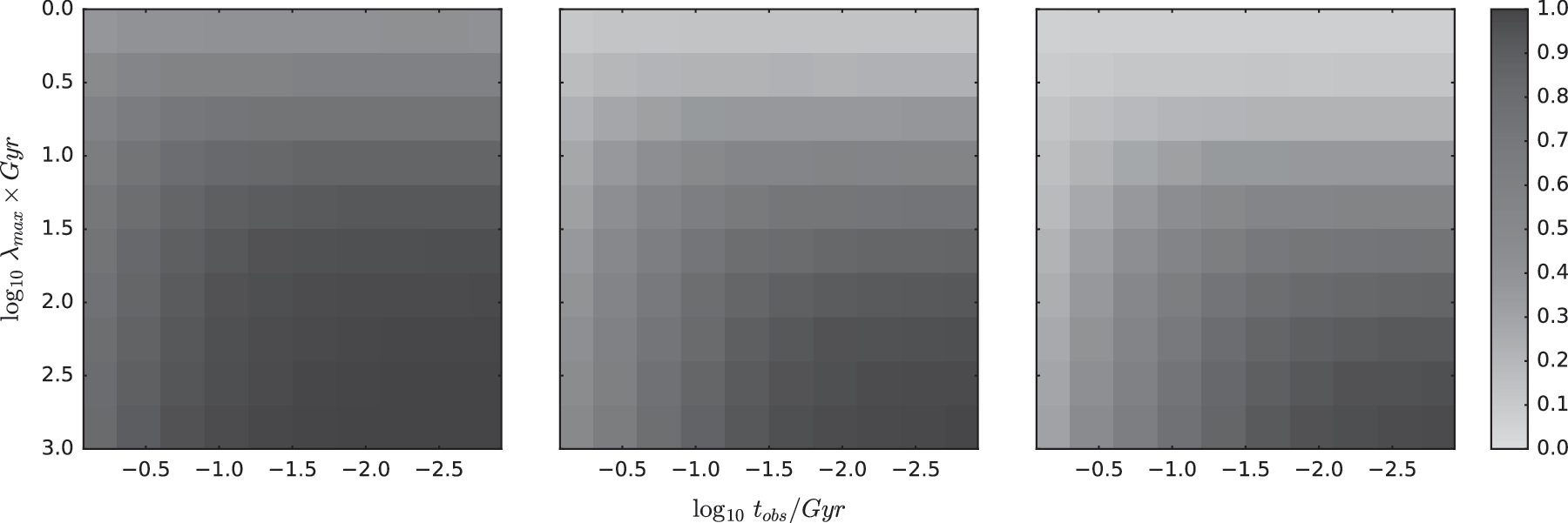
The three plots show the predicted ratio of planets with life given the situation on the Earth. From left to right panel, λ _min = 10⁻³ Gyr⁻¹, 10⁻¹¹ Gyr⁻¹, and 10⁻²² Gyr⁻¹. In each panel, we vary t _obs (x axis) and λ _max (y axis).

As Figure 3 makes clear, changing λ _min leads to a significant decrease in the expected success yield. For these reasons, the experiment 3 information gains presented here are highly sensitive to the assumed values of λ _min. We note that this was not the case in experiments 1 and 2, where we verified that varying λ _min to 10⁻¹¹ Gyr⁻¹ or 10⁻²² Gyr⁻¹ did not significantly impact the shape of the posteriors and only slightly affected the scaling of the information gain plots. For this reason, in what follows, we limit our discussion to being largely a qualitative one.

3.3.3. Qualitative impacts on the λ posterior and information gain

In the right panel of Figure 4, the dark lines show four example posteriors for λ for N = 10, 50, 200, and 1000. The dark lines all assume M/N = 30%. If 30% of the planets harbor life, then this implies that a λ of 0.3/5 Gyr⁻¹ and this is indeed where the posteriors all peak. The peakiness of the posterior naturally increases as it becomes conditioned upon larger samples of data.

FIG. 4.

The left panel shows information gain calculated as we increase the number of observed exoplanets. The right panel gives the detailed posterior distribution of λ for different ratios.

The leftmost lines show the case of no detections, M = 0, which strongly opposes our prior expectation of a high rate. However, because these are essentially null detections, the posterior peaks at λ _min and does not converge to a single quasi-Gaussian shape. For this reason, the posterior does certainly lead to a large information gain but not maximal.

However, if M = N, shown by the bottom lines, the information gain is minimal. As explained in detail earlier, this results from our high prior expectation of λ anyway, conditioned upon the Earth's early start to life. Adding more data only re-enforces this belief leading to minor gains in information content. Furthermore, as with the M = 0 case, the posterior peaks at a prior bound, in this case λ _max, and thus does not represent a converged constrained datum.

The argument made above does not include effects regarding the sample inclusion though. For example, if all Earth-like planets surveyed show evidence for life, there would be an opportunity to learn about abiogenesis in a different way by gently expanding the sample to suboptimal worlds and observing when the success rate decreases. This is not formally encoded within our model and represents just one of the ways that a large sample of exo-life detections would lead to large gains in understanding of abiogenesis, even if not significantly improving our inference of the abiogenesis rate of Earth-like worlds.

4. Discussion

In this work, we have sought to understand how three different experimental approaches would be expected to inform our knowledge of the rate of abiogenesis, λ, on Earth-like worlds. Our approach adopts the Bayesian formalism of Spiegel and Turner (2012) as a means for deriving the probability distribution of λ conditioned upon some observation of the earliest evidence for life (t _obs) and some choice for the prior. As discussed in the study of Spiegel and Turner (2012), the resulting posteriors are highly influenced by the choice of prior, and thus, an absolute inference of the posterior is somewhat unachievable. Instead, our article focuses on the relative gain in information acquired as new experiment evidence is introduced into the problem across a range of plausible input parameters.

Our Bayesian informatics approach seeks to understand exactly how the λ posterior changes in response to new experimental constraints, and whether there are certain experiments or parameter regimes, which can be concluded to either be negligibly informative or vice versa greatly informative.

Our work focuses on three thought experiments, which could be plausibly conducted at present or in the near future: (1) paleontological evidence for an earlier start to life, (2) Monte Carlo experiments seeking to create a laboratory abiogenesis event, and (3) a survey of exoplanets for biosignatures. To quantify the information gained from each experiment, we used the KLD or relative entropy to calculate the difference between the original and the new λ posterior. Additionally, we have performed detailed analyses of the resulting posteriors in an attempt to understand how their morphologies are sculpted by new constraints.

Without knowledge of the correct limits on the prior (or indeed the shape of the prior), it is not possible to unambiguously claim that any of these experiments will always be superior/inferior to the others. Despite this, there are general trends that emerge from our thought experiments. These are briefly summarized in Figure 5, and we urge the reader to explore the more detailed accounts of each found within this article.

FIG. 5.

Summary chart of some key general results found in this work.

We highlight a couple of important general trends. First, it is nonintuitive that an exoplanet survey detecting many instances of life can be highly uninformative in certain regimes. This is because for certain choices of the prior, the early start to life on the Earth leads to an expectation that all Earth-like planets are inhabited, thus new detections do not significantly affect the posterior. As highlighted earlier though, clearly such a result could be greatly informative if the sample is extended beyond Earth-like worlds to include more exotic locations, echoing the conclusion of Lenardic and Seales (2018) but for different reasons.

Second, we have ignored the possibility of a successful laboratory abiogenesis in this work and instead assumed that they only yield null results and thus an upper limit on λ. This is motivated by the assumption that the ability to create life in the laboratory, in a reproducible experiment, would provide an enormous amount of information that would make direct comparisons somewhat meaningless to the other experiments. This is related to the possibility of paleontology/paleogenetics finding unambiguous evidence for a second abiogenesis at early times, which we also did not explicitly consider.

A general trend we highlight is that unless abiogenesis occurs in the laboratory, the biological and paleontological experiments are conditioned upon the same datum—the earliest evidence for life on the Earth—and thus both yield only lower limits on λ. In contrast, exoplanet surveys will, in general, yield peaked posteriors constrained from both sides, that is, a measurement rather than a limit. This is important to emphasize as this is not fully captured by simply comparing the relative entropies between posteriors.

A final point we emphasize is that paleontology in particular has regimes in which essentially no information is gained. For reasons discussed in detail earlier, this occurs when t _obs. Since there is no agreed value for λ _max, we are unable to infer what the corresponding time really is, but it is important to note that even a very early start to life can, for some choices of λ _max, make us none the wiser about abiogenesis.

Being the first effort at a Bayesian informatics analysis of abiogenesis, we acknowledge that there are outstanding issues that we have not been able to address in detail here. First, we did not conduct a full exploration of the effect of changing λ _min, largely since we could not conceive of a direct empirical way of constraining it. Another issue is that we have assumed that λ follows a universal distribution for all exoplanets and at all times, while of course we should expect that it will change with different environments. This was largely done as a simplifying assumption, following the study of Spiegel and Turner (2012), and is partly mitigated by our assumption that only “Earth-like” worlds are included in an exoplanet survey. This problem might be better solved in the future with hierarchical models, which were not explored here. Finally, we have assumed that experiment 3 is actually feasible, which remains somewhat unclear. Specifically, we assume that life can be unambiguously detected or ruled out on a planet from remote observations. A suggestion for future work would be to change this hard binary flag to a softer probability, implying a more complicated model such as again a hierarchical model.

Together, we generally find that all the experiments can certainly yield constraints on λ and in nonoverlapping ways. A laboratory abiogenesis event would be such an informative experiment that even if it could be argued that the information gains from null results are negligible, there is a strong case to conduct the experiment regardless. Similarly, early starts to life, while they may not formally improve λ, do clearly provide information about the conditions in which life began, and this is not formally encoded in our model. If an actual measurement of λ is desired, rather than a limit, we would argue that the exoplanet survey is the most direct way to infer this. Moreover, the ability to expand to non-Earth-like worlds can probe different conditions and thus offer an orthogonal type of information. Altogether, all three experiments deserve our attention and resources in our quest to answer one of modern science's greatest questions.

Footnotes

Author Disclosure Statement

No competing financial interests exist.

Abbreviations Used

References

Allwood

A.C.

(2016) Geology: evidence of life in Earth's oldest rocks. Nature, 537:500–501.

Anderson

T.W.

and Darling

D.A.

(1952) Asymptotic theory of certain “goodness-of-fit” criteria based on stochastic processes. Ann Math Stat, 23:193–212.

Bottke

W.F.

, Vokrouhlický

, Marchi

, Swindle

, Scott

E.R.D.

, Weirich

J.R.

, and Levison

(2015) Dating the Moon-forming impact event with asteroidal meteorites. Science, 348:321–323.

Carter

(1983) The anthropic principle and its implications for biological evolution. Philos Trans Roy Soc London A, 310:347–363.

Cassan

, Kubas

, Beaulieu

J.-P.

, Dominik

, Horne

, Greenhill

, Wambsganss

, Menzies

, Williams

, Jorgensen

U.G.

, Udalski

, Bennett

D.P.

, Albrow

M.D.

, Batista

, Brillant

, Caldwell

J.A.R.

, Cole

, Coutures

Ch.

, Cook

K.H.

, Dieters

, Dominis Prester

, Donatowicz

, Fouqué

, Hill

, Kains

, Kane

, Marquette

J.-B.

, Martin

, Pollard

K.R.

, Sahu

K.C.

, Vinter

, Warren

, Watson

, Zub

, Sumi

, Szymański

M.K.

, Kubiak

, Poleski

, Soszynski

, Ulaczyk

, Pietrzyński

, and Wyrzykowski

(2012) One or more bound planets per Milky Way star from microlensing observations. Nature, 481:167–169.

Dalrymple

G.B.

(2001) The age of the Earth in the twentieth century: a problem (mostly) solved. Geol Soc London Special Publ, 190:205–221.

Darwin

(1859) On the Origin of Species by Means of Natural Selection. J. Murray, London.

Dodd

M.S.

, Papineau

, Grenne

, Slack

J.F.

, Rittner

, Pirajno

F. O

, 'Neil

, and Little

C.T.S.

(2017) Evidence for early life in Earths oldest hydrothermal vent precipitates. Nature, 453:60–64.

Drake

F.D.

(1965) The radio search for intelligent extraterrestrial life. In Current Aspects of Exobiology, edited by Mamikunian

and Briggs

M.H.

, Pergamon Press, Inc., New York, pp. 323–345.

10.

Dressing

C.D.

and Charbonneau

(2015) The occurrence of potentially habitable planets orbiting M Dwarfs estimated from the full Kepler dataset and an empirical measurement of the detection sensitivity. Astrophys J, 807:45–67.

11.

Foreman-Mackey

, Hogg

D.W.

, and Morton

T.D.

(2014) Exoplanet population inference and the abundance of earth analogs from noisy, incomplete catalogs. Astrophys J, 795:64–75.

12.

Kolmogorov

(1933) Sulla determinazione empirica di una legge di distribuzione. G Ist Ital Attuari, 4:83–91.

13.

Kullback

and Leibler

R.A.

(1951) On information and sufficiency. Ann Math Stat, 22:79–86.

14.

Künsch

H.R.

(2013) Particle filters. Bernoulli, 19:1391–1403.

15.

Lacki

B.C.

(2016) The log log prior for the frequency of extraterrestrial intelligences. arXiv, 1609:05931.

16.

Léger

, Mariotti

J.M.

, Mennesson

, Ollivier

, Puget

J.L.

, Rouan

, and Schneider

(1996) Could we search for primitive life on extrasolar planets in the near future?. Icarus, 123:249–255.

17.

Lenardic

and Seales

(2018) Different is more: the value of finding an inhabited planet that is far from Earth 2.0. arXiv, 1801:09146 [astro-ph.EP].

18.

Lineweaver

C.H.

and Davis

T.M.

(2002) Does the rapid appearance of life on Earth suggest that life is common in the Universe?. Astrobiology, 2:293–304.

19.

Metropolis

(1953) Equation of state calculations by fast computing machines. J Chem Phys, 21:1087–1092.

20.

Miller

S.L.

and Urey

H.C.

(1959) Organic compound synthesis on the primitive Earth. Science, 130:245–251.

21.

Rauscher

B.J.

, Bolcar

M.R.

, Clampin

, Domagal-Goldman

S.D.

, McElwain

M.W.

, Moseley

S.H.

, Stahle

, Stark

C.C.

, and Thronson

H.A.

(2015) AT-LAST detector needs for direct spectroscopic biosignature characterization in the visible and near-IR. SPIE, 9602:96020D.

22.

Robitaille

T.P.

and Whitney

B.A.

(2010) The present-day star formation rate of the Milky Way determined from Spitzer-detected young stellar objects. Astrophys J Lett, 710:L11–L15.

23.

Scharf

and Cronin

(2016) Quantifying the origins of life on a planetary scale. Proc Natl Aacd Sci U S A, 113:8127–8132.

24.

Schopf

W.J.

, Kudryavtsev

A.B.

, Czaja

A.D.

, and Tripathi

A.B.

(2007) Evidence of Archean life: stromatolites and microfossils. Precambrian Res, 158:141–155.

25.

Seager

(2014) The future of spectroscopic life detection on exoplanets. Proc Natl Acad Sci U S A, 111:12634–12640.

26.

Simpson

(2017) The longevity of habitable planets and the development of intelligent life. Int J Astrobiol, 16:266–270.

27.

Smirnov

(1948) Table for estimating the goodness of fit of empirical distributions. Ann Math Statist, 19:279–281.

28.

Sober

(2008) Evidence and Evolution: The Logic Behind the Science. Cambridge University Press, Cambridge, UK.

29.

Spiegel

D.S.

and Turner

E.L.

(2012) Bayesian analysis of the astrobiological implications of life's early emergence on Earth. Proc Natl Acad Sci U S A, 109:395–400.

30.

Tasker

, Tan

, Heng

, Kane

, Spiegel

, Brasser

, Casey

, Desch

, Dorn

, Hernlund

, Houser

, Laneuville

, Lasbleis

, Libert

A.-S.

, Noack

, Unterborn

, and Wicks

(2017) The language of exoplanet ranking metrics needs to change. Nat Astron, 1:42–46.

31.

Valley

J.W.

, Cavosie

A.J.

, Ushikubo

, Reinhard

D.A.

, Lawrence

D.F.

, Larson

D.J.

, Clifton

P.H.

, Kelly

T.F.

, Wilde

S.A.

, Moser

D.E.

, and Spicuzza

M.J.

(2014) Hadean age for a post-magma-ocean zircon confirmed by atom-probe tomography. Nat Geosci, 7:219–223.

32.

Wessen

P.S.

(2010) Panspermia, past and present: astrophysical and biophysical conditions for the dissemination of life in space. Space Sci Rev, 156:239–252.

33.

Wilde