Simulating Serpentinization as It Could Apply to the Emergence of Life Using the JPL Hydrothermal Reactor

Abstract

The molecules feeding life's emergence are thought to have been provided through the hydrothermal interactions of convecting carbonic ocean waters with minerals comprising the early Hadean oceanic crust. Few laboratory experiments have simulated ancient hydrothermal conditions to test this conjecture. We used the JPL hydrothermal flow reactor to investigate CO₂ reduction in simulated ancient alkaline convective systems over 3 days (T = 120°C, P = 100 bar, pH = 11). H₂-rich hydrothermal simulant and CO₂-rich ocean simulant solutions were periodically driven in 4-h cycles through synthetic mafic and ultramafic substrates and Fe>Ni sulfides. The resulting reductants included micromoles of HS⁻ and formate accompanied possibly by micromoles of acetate and intermittent minor bursts of methane as ascertained by isotopic labeling. The formate concentrations directly correlated with the CO₂ input as well as with millimoles of Mg^{2
+} ions, whereas the acetate did not. Also, tens of micromoles of methane were drawn continuously from the reactor materials during what appeared to be the onset of serpentinization. These results support the hypothesis that formate may have been delivered directly to a branch of an emerging acetyl coenzyme-A pathway, thus obviating the need for the very first hydrogenation of CO₂ to be made in a hydrothermal mound. Another feed to early metabolism could have been methane, likely mostly leached from primary CH₄ present in the original Hadean crust or emanating from the mantle. That a small volume of methane was produced sporadically from the ¹³CO₂-feed, perhaps from transient occlusions, echoes the mixed results and interpretations from other laboratories. As serpentinization and hydrothermal leaching can occur wherever an ocean convects within anhydrous olivine- and sulfide-rich crust, these results may be generalized to other wet rocky planets and moons in our solar system and beyond.

1. Introduction

Corliss and collaborators (1981) were the first to suggest that life may have originated in the kind of methane- and hydrogen-bearing submarine hydrothermal systems feeding the “Black Smokers” first reported by Welhan and Craig (1979), Spiess et al. (1980), and Hekinian et al. (1980). These hydrothermal fluids were considered the result of magmatic heating of circulating seawater at ocean spreading ridges (Cann et al., 1985). This autogenic hypothesis met fierce opposition, with Miller and Bada (1988) in particular arguing that such high temperatures in the vents would allow neither synthesis nor the survival of organic compounds. However, other hydrothermal systems were known to develop within ophiolites—obducted or uplifted paleocean floors—where temperatures of the effluents are not only much lower but also highly alkaline (Neal and Stanger, 1984). While these particular fluids are exhaling into shallow water or onto dry land, it was reasoned that similar systems would also have developed on ocean floors (Russell et al., 1989). The discovery of the Lost City hydrothermal vent field (LCHF) 15 km west of the North Atlantic Rift appeared to satisfy this expectation (Kelley et al., 2001, 2005). Such alkaline exhalations, considered a feature of brittle fracturing at slow spreading centers, are mainly driven by exothermic serpentinization (Lowell and Rona, 2002). The process is initiated as faults in the stressed mafic ocean crust allow water to gravitate downward, increasing effective stress as a result of hydrostatic pressure; hydrating and hydrolyzing olivine to serpentinite and, as a result, driving the cracking front to the brittle-ductile boundary (Russell et al., 1995; Amiguet et al., 2014). The system as a whole behaves as an exothermic, autocatalytic cracking engine, with extra heat provided by the occasional intrusion of magmatic sills at depth (Cottrell, 1979; Branscomb et al., 2017; Malvoisin et al., 2017; Olive and Crone, 2018).

The convective systems feeding such submarine alkaline springs appear to operate at or below 150°C (Fig. 1) (Proskurowski et al., 2006). Shallow, secondary convection cells involving the carbonic ocean waters also form (Fig. 1). These geophysical conditions are not unlike those that would have been operating around the magmatic plumes likely to have been the main mechanism of heat loss on the early Earth (Lowell and Rona, 2002; Bédard, 2006; Emmanuel and Berkowitz, 2006; Artemieva and Thybo, 2013; Moore and Webb, 2013; Jian et al., 2017). Exhaling into the Hadean iron-rich ocean, the alkaline vent waters would have had the effect of precipitating this metal, and other transition elements such as sulfides and oxyhydroxides (Kump and Seyfried, 2005; White et al., 2015; Russell, 2018).

FIG. 1.

Schematic representation of the alkaline hydrothermal vent model for the emergence of life on the early Earth (modified after figure 1 of Russell and Hall, 1997; the serpentinization photo was kindly contributed by Dr. Laurie Barge: see cover). The experiments reported here simulate rock:water interactions between the simulated Hadean ocean crust and convecting CO₂-bearing ocean waters, both at depth and during secondary convection. Simulated reactions at the mound margins itself are reported in White et al. (2015); Russell (2018); Wang et al. (2019); and Barge et al. (2019). Color images are available online.

A simplified serpentinization reaction (i) to illustrate the origin of the hydrogen at Lost City and elsewhere is taken from the work of Proskurowski et al. (2008):

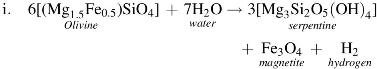
Such serpentinizing hydrothermal systems appear to produce effluents rich not only in hydrogen and formate but also in methane. Under these conditions, any entrained organic molecules would also remain stable (Shock, 1990, 1992).

1.1. Possible significance to the emergence of life

Submarine alkaline hydrothermal vent (AHV) systems may have been responsible for life's emergence on Earth (figure 1; Russell et al., 1989; Russell and Hall, 1997; Russell and Hall, 2006.; Lane, 2010; Mielke et al., 2011; Branscomb and Russell, 2018). In this scenario, the warmer alkaline hydrothermal fluids rise buoyantly through convection, driven by serpentization, toward the ocean crust where they are subsequently cooled as they meet CO₂-rich ocean. There, hydrogen- and methane-rich waters mixed with mildly acidic ocean waters bearing dissolved CO₂, which served as a low-potential electron acceptor as well as a source of carbon for early metabolic reactions.

The assumption that CO₂ could be reduced to methane in these conditions as an abiotic analogue of methanogenesis has led to mixed experimental results and uncertainty (Horita and Berndt, 1999; Seewald et al., 2006; Martin and Russell, 2007; Proskurowski et al., 2008; Etiope and Ionescu, 2015). While several studies of alkaline systems showed that CO, CO₂, or HCO₃ ⁻ species can be reduced by iron/nickel alloys to form methane at low temperatures (<200°C), many hydrothermal experiments mimicking serpentinization (McCollom and Donaldson, 2016) have failed to convert CO₂ to methane, or indeed to record reduction beyond formate. Nevertheless, others have presented evidence that methane can be reduced from CO₂ during serpentinization during weathering of olivine at temperatures between 30°C and 70°C (Neubeck et al., 2011; Suda et al., 2014). To complicate matters further, both abiogenic methane and formate are observed in fluids at the LCHF, although according to Lang et al. (2010, 2012, 2018), both are derived from depth, perhaps unrelated to the serpentinization reaction per se.

Unlike present-day mounds dominated by oxide species precipitated in a less alkaline (pH 7.9) ocean (Kelley et al., 2005; Pisapia et al., 2017; Price et al., 2017), ancient hydrothermal mounds are thought to be comprised primarily of brucite-like green rust (∼Fe^II ₄Fe^III ₂[OH]₁₂CO₃·3H₂O), accompanied by amorphous silica, mackinawite (∼FeS), greigite (∼Fe₃S₄), and, perhaps, ephemeral dolomite (CaMg(CO₃)₂) (Macleod et al., 1994; Russell and Hall, 1997; White et al., 2015; Gourcerol et al., 2016; Tosca et al., 2016; Gäb et al., 2017; Halevy et al., 2017; Russell et al., 2017; Russell, 2018). In this ancient system, iron sulfides lining the interior walls of the chimneys may have acted as catalysts and reactants for CO₂ reduction and could have retained any organic molecules so produced to allow further reactions, acting like early forms of protohydrogenase or carbon monoxide dehydrogenase (Russell et al., 2003; McGlynn et al., 2009). Dictated by the thermodynamic conditions, such reactions would allow for either methane or acetate synthesis to occur (Amend and Shock, 2001) and formate would be produced as an intermediate. Notionally, in these experiments, the catalytic reduction of CO₂ by H₂ to methane over iron sulfide catalysts predicted to be present in ancient submarine hydrothermal mounds is to be expected (White et al., 2015):

While several previous studies have attempted to illuminate how early life emerged on the Earth from hydrothermal systems, abiotic organic synthesis during serpentinization—if indeed it happens beyond formate—remains poorly understood and largely undemonstrated (Shock, 1990; Schoonen et al., 1999; Amend and Shock, 2001; Amend and McCollom, 2009; McCollom and Bach, 2009; Shibuya et al., 2010; Reeves et al., 2014). Few laboratory simulations have investigated the ability for the alkaline hydrothermal system to supply organic molecules under the appropriate hydrothermal temperatures and pressures, and in the presence of appropriate catalysts, although Herschy et al. (2014) generated formate in a membrane reactor. These authors have also claimed to have synthesized formaldehyde, although one should caution that the gas is ubiquitous and may thus have been a contaminant (Salthammer, 2013).

Here, we describe an investigation of the alkaline vent model for life's emergence focused on the presumed reduction of CO₂ during simulated serpentinization. We show that CO₂ does reduce to formate, possibly minor acetate, and, sporadically, even methane. The results force amendments to the AHV theory, suggesting, after the work of Windman et al. (2007), that hydrogen and CO₂ were processed within the ocean crust to produce formate (one free-energy-releasing additive to the first autotrophic pathways), along with abiotic methane produced mainly at depth and entrained in the hydrothermal fluids (Russell, 2018; figure 1). In these experiments, synthetic komatiite (ultramafic simulant), basaltic rock wool (basalt simulant), and pentlandite (iron sulfide) were selected as the reactor bed materials to mimic both the starting conditions for, and the progenitors of, serpentinization.

2. Thermodynamic Modeling

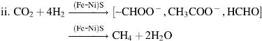
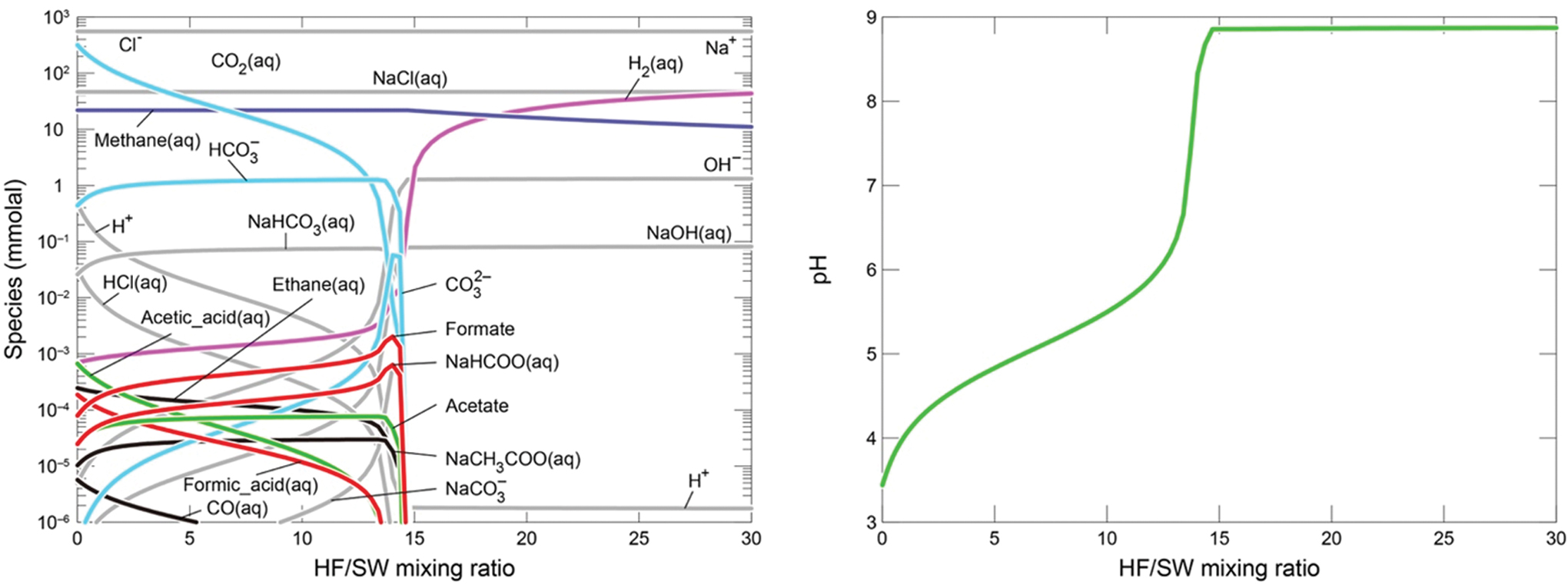
We develop expected outputs from the experiments from thermodynamic modeling, with an emphasis on methane generation (Fig. 2 cf. Experiment 2; Fig. 3 cf. Experiment 3). Mixing between the alkaline fluid and CO₂-rich seawater was simulated by using the REACT module in Geochemist's Workbench with the default thermodynamic database (Bethke, 2007) as investigated by Shibuya et al. (2016). Seawater solutions were equilibrated by ∼10 and ∼1 bar of CO₂ gas, corresponding to ∼340 mmol/kg and 34 mmol/kg of total CO₂ ( = [CO_2aq] + [HCO₃ ⁻] + [CO₃ ²⁻] + [NaHCO_3aq] + [NaCO₃ ⁻]) concentrations, respectively. For both seawater and hydrothermal solutions, we assumed H₂ concentrations of ∼88 mmol/kg because the solutions are pressurized with 100 bar of H₂ gas during the experiments (see Section 3). Mixing reactions at 120°C predict maximum methane concentrations of 22 mmol/kg in the regions with low ratios of hydrothermal fluid to seawater (HF:SW) for both experiments (Figs. 2 and 3). Acetic acid species (e.g., acetic acid, acetate and NaCH₃COO_aq) and formic acid species (formic acid, formate, and NaCOOH) can also form in the regions with low HF:SW, but their concentrations are generally less than 1 μmol/kg. However, if methane and other normal alkanes are suppressed (kinetically limited, e.g. McCollom and Seewald, 2001), concentrations of these “intermediate” organic carbon species may be elevated. Solid reactants likely to precipitate upon mixing of hydrothermal fluid with cold seawater were not included in this modeling. Instead, we look to the experimental results reported below to assess the influence of solid materials.

FIG. 2.

Dissolved compositions predicted by thermodynamic calculations of mixing between alkaline fluid and CO₂-rich seawater (10 bar CO₂) at 120°C (cf. Experiment 2 reported results). Color images are available online.

FIG. 3.

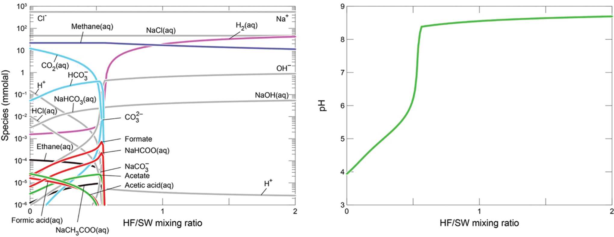
Dissolved compositions predicted by thermodynamic calculations of mixing between alkaline fluid and CO₂-rich seawater (1 bar CO₂) at 120°C (cf. Experiment 3 reported in results). Color images are available online.

3. Experimental Design, Preparation, and Analysis Methods

The previously reported JPL hydrothermal reactor (Mielke et al., 2010) was used in renovated form, as illustrated in Fig. 4. The general experimental design was as follows: ground pentlandite and komatiite were mixed together and placed inside a reactor tube. On either end of the tube, rock (basaltic) wool (calcium-magnesium silicate) was inserted to hold the pentlandite/komatiite mixture in place as well as simulate one of the ocean crust constituents. H₂-rich alkaline fluid was prepared as a hydrothermal simulant, and CO₂-rich acidic fluid was prepared as an ancient Hadean ocean simulant. The temperature of the fluids and reactor bed was controlled to mimic alkaline hydrothermal temperatures and the fluids were kept in pressurized vessels to mimic ocean floor pressures. Maintained at high pressure and controlled by valves, the two fluids were switched alternately to flow through the reactor bed, each for 4 h to provide sufficient time for the fluid to fully dominate the reactor bed. Four hours is the time it takes the fluid to completely pervade the reactor bed.

FIG. 4.

Diagram of the hydrothermal reactor modified from Mielke et al. (2010) (see text for description). TLS. Color images are available online.

3.1. Reactor design and operation

The modified JPL hydrothermal reactor system consists of two 3.8 L pressure vessels made from 316 electro-polished stainless steel (316epSS), which serve as reservoirs for simulated seawater and hydrothermal fluid. The hydrothermal reactor provides a constant flux condition similar to that feeding hydrothermal mounds, which themselves result from constant effluent flow from beneath the seafloor. Thus, the reactor simulates hydrothermal fluid pressures and temperatures (∼100 bar and 100–150°C) as they interact with the CO₂-bearing Hadean ocean waters. As remarked upon above, H₂ and CO₂ fluids were alternatingly fed continuously at 4-h intervals to a reaction chamber containing the solid materials simulating minerals at, and immediately beneath, the alkaline mound. This also simulates the mixing of carbonic seawater with more reducing hydrothermal fluid just beneath the mound.

Temperatures were maintained by using strip sensing thermal ribbons (Minco^®) and measured with multiple K-type thermocouples (accuracy of ±1 K) placed within the insulated heating jacket of the main reactor and logged automatically every 15 min. The pressure in each tank was monitored to an accuracy of ±0.01 torr with a dedicated capacitance monometer (Baratron^®) connected to a PDR2000A pressure readout (MKS^®). Carbon dioxide and hydrogen gases were introduced near the bottom of the tanks to ensure full gas/water exchange before each run.

The reactor flow rate was adjusted to ∼15 mL/h. The resulting solutions were fed into nitrogen-purged, acid-washed, 20 mL crimp-top vials. The vials were switched every hour for continuous sampling (Fig. 4).

Reactions are expected to mimic convective flow through the crust as well as in the complex environment at, and just beneath, the hydrothermal edifice. Freshly autoclaved minerals were loaded before each experiment and were thoroughly characterized before and after the reaction. Previously, we reported results from reactor experiments simulating hydrothermal conditions using mafic and iron sulfide minerals (Mielke et al., 2010). Here, we use synthetic and field minerals expected within the mafic crust as well as beneath and within the compartments of the AHVs (Yoshizaki et al., 2009). Specifically, in all experiments, we used synthetic komatiite to simulate ultramafic compositions, and calcium/magnesium silicate to simulate mafic rock. Pentlandite (iron/nickel sulfide) was added as a catalyst and reactant to simulate iron sulfides predicted to be present beneath and in ancient alkaline vents (Russell et al., 2010; Barnes and Fiorentini, 2012; Shanks and Thurston, 2012).

3.2. Experimental conditions

Table 1 summarizes the experimental conditions. Hydrogen effluents from the simulated ancient hydrothermal systems were tested for their propensity to react with CO₂-rich fluids to produce any putative simple organic acids, aldehydes, and methane as first steps to the emergence of life. The control experiment (Experiment 1) excluded CO₂ from the ocean tank, providing a background test for methane and/or dissolved organic molecule leaching from the reactor charge. Experiments 2 and 3 were conducted under the same conditions but different CO₂ concentrations. All three experiments were conducted in the presence of ∼100 bar (88 mmol/kg) H₂, simulating the H₂-rich AHV effluents at seafloor pressures.

Table 1.

Parameters for Hydrothermal Reactor Experiments

Experiment 1
	Tank 1 (hydrothermal fluid)	Tank 2 (ocean fluid)
PH₂	100 bar	100 bar
PCO₂	0 bar	0 bar
pH	11.0 (titrated w/NaOH)	5.0 (titrated w/HCl)
T°C	120	120
NaCl (mM)	600	600

Experiment 2
PH₂	100 bar	100 bar
PCO₂	0 bar	10 bar
pH	11.0 (titrated w/NaOH)	5.0 (titrated w/HCl)
T°C	120	120
NaCl (mM)	600	600

Experiment 3
PH₂	100 bar	100 bar
PCO₂	0 bar	1 bar
pH	11.0 (titrated w/NaOH)	5.0 (titrated w/HCl)
T°C	120	120
NaCl (mM)	600	600

The ocean fluid simulant was titrated to pH 5.0 using 0.5 M HCl to mimic the pH conditions assumed at the submarine alkaline vent. We used isotopically labeled CO₂ (99.99% enriched in ¹³C) as the carbon feedstock in Experiment 3 to ensure that end products were not contaminated by, or derived from, background sources of carbon.

3.3. Preparation of materials and solutions

Solid materials were prepared as follows. Calcium/magnesium silicate (Minwood 1200; Industrial Insulation Group, AL) was baked at 500°C overnight to remove residual organic molecules. Komatiite (∼Mg₂SiO₄) was synthesized from reagents with an electric furnace as described by Yoshizaki et al. (2009) and Ueda et al. (2016). Solid materials were ground into powders to maximize surface area for reaction with fluids. Each reactor run used 60.0 g of komatiite, ground into powder with a mortar and pestle, then transferred to a glass vial, and placed in a dry box under inert (N₂) atmosphere. To remove any residual organics, the powder was rinsed once with 1 M HCl and subsequently rinsed up to 10 times with Milli-Q H₂O until the solute returned to a neutral pH (∼6.5). Pentlandite [(Fe,Ni)₉S₈] was obtained from Alexo Mine, Dundonald Township Timmins Area, Cochrane District, Ontario, Canada (Thomson et al., 1957). Each reactor run used 30.0 g of pentlandite, also ground into a powder and stored in a sealed N₂-purged glass vial. Calcium/magnesium silicate was packed at the base of the reactor and on top of the komatiite and pentlandite mixture to hold the mixture in place while allowing liquid to flow through the reactor.

To prepare the tank solutions, the two 3.5 L Milli-Q (18.2 Ω) H₂O solutions were initially prepared in glass beakers, sealed with parafilm, and purged with nitrogen for >3 h to remove dissolved O₂ and CO₂. NaCl was added to both solutions to make a 600 mM NaCl concentration, based on the assumption that the Hadean ocean was sourced from high-temperature ultramafic springs (Wetzel and Shock, 2000). For the alkaline hydrothermal effluent simulant, one solution was titrated to pH = 11 by using 0.1 M NaOH in 600 mM NaCl aqueous solution. For the Hadean ocean simulant, the pH of the solution was adjusted through the addition of CO₂ (g) after loading both solutions into the reactor vessels (Table 1). On dissolving in water, CO₂ (g) would form carbonic acid and bicarbonate, and thus, the resulting pH of the ocean simulant was between ∼pH 5 and 7, depending on the CO₂ gas pressure (cf. Kusakabe et al., 2000).

Because H₂ (g) is explosive when reacted with O₂ (g) under pressure, precautions were taken to ensure the complete removal of O₂ in the reactor system as expected of Hadean conditions, before introducing H₂. Nitrogen was bubbled through the reactor tanks and reactor bed at 14 bar gauge pressure (in excess of atmospheric pressure) and at ambient temperatures three times. The head space was evacuated with a turbo vacuum pump between each nitrogen flush. Following the final pumping sequence, hydrogen gas was introduced to the tanks at a pressure of 800 psi and raised to 1500 psi (∼100 bar) concurrently to prevent overpressurization as temperatures were raised to 120°C.

3.4. Solid inorganic analysis

Reactor bed materials were analyzed before and after each experiment to determine the alteration products. After each reactor experiment, reactor bed materials were pulled from the reactor bed and immediately placed in a crimped, nitrogen-purged glass vial. Reactor bed materials were divided into ∼20–25 aliquots and analyzed with environmental scanning electron microscope/energy dispersive spectrometer (ESEM/EDS) and Raman spectroscopy.

The composition and mineralogy of reactor bed materials were determined before and after the experiments with a Phillips XL30 ESEM with attached EDS system. For ESEM analyses, samples were placed on an aluminum tab, which was inserted into the ESEM with a water vapor pressure of 3.8 torr, an accelerating voltage of 20 kV, and a working distance of 10.2 mm. The gaseous secondary electron detector was also used at a chamber pressure of 3.8 torr to allow imaging without subsequent coating steps. The spot analysis feature was used in energy-dispersive X-ray spectrometry (EDAX, Inc.) to analyze X-ray signals with the Genesis software program. Between 30 and 50, spectra were collected to the determine bulk composition of each sample before and after alteration.

Raman spectra of pre- and postexperiment samples were obtained on a LabRam HR (Horiba Jobin Yvon) with use of a 532 nm laser and 600 g/mm grating with a resolution of ∼2 cm⁻¹. All samples were placed in a nitrogen-purged LinkAm LTS350 cryochamber to prevent oxidation by ambient air. The cryochamber was placed on a three-axis-motorized stage and the sample illuminated through a sapphire window. The instrument was calibrated by using the 520 cm⁻¹ silicon line and zero order. Point maps were collected for each sample analyzed, yielding ∼100 spectra per sample. The RRUFF Raman database (Downs, 2006) was used to identify mineral phases based on observed peak shift locations.

Pentlandite samples were crushed with a mortar and pestle and analyzed by ESEM, Raman, and X-ray diffraction spectroscopy (XRD). Samples of unaltered and altered pentlandite were analyzed with a Siemen's D500 X-ray diffractometer equipped with a Cu anode tube Peltier cooled Kevex Si(Li) (lithium-drifted silicon) X-ray detector and a Co-Ka Fe-filter. Minerals were identified by reference to the 2009 ICDD database for organic and inorganic phases, in conjunction with the JADE PLUS (v9.1.1) XRD analysis program.

3.5. Aqueous inorganic analysis

To avoid oxidation from exposing the solutions to air, the pH of each solution collected from reactor experiments was determined in situ. A needle probe (Microelectrodes^®, 16 G) was used to directly measure pH in the 20 mL crimped-top sample vials, or ∼3 mL of solution was extracted via syringe and placed into a 5 mL vial with pH measured immediately by a standard pH probe (Thermo Scientific^®).

The concentrations of dissolved ions in sample solutions were determined by inductively coupled plasma atomic emission spectroscopy (ICP-AES; Thermo Scientific iCAP 6300a). Samples and standards were prepared in glassware, and sample vials soaked in ∼1 M HCl overnight, triple rinsed with Milli-Q H₂O (18.2 Ω), and baked at ∼200°C. Standard solutions were prepared from the same 1 M HCl stock solution and prepared gravimetrically to create a calibration curve for ICP analysis. Standards were prepared from 1000 ppm stock solutions of S, Mo, Ni, Fe, Si, Mg, K, Ca, and Al (assurance grade; SPEX Certiprep, Inc.). Ion concentrations in each standard were computed from gravimetric measurements and assimilated into the iTEVA Analyst software to create a calibration curve. The software was programmed to recalibrate after every 10 analyses using the prepared standard solutions. Each sample was analyzed three times by ICP-AES, and standard deviations were calculated from triplicate runs.

3.6. Aqueous organic analysis

Ion exclusion chromatography (IEC) and conductivity were used to detect formate and acetate—a method that requires a desalting step to estimate concentrations ranging from ∼1 to 150 μM. We followed the methods of Lang et al. (2010), with the exception of using valeric acid instead of adipic acid as an internal standard for desalted solutions. For desalting, solutions were passed through Dionex^® Ba/Ag/H 2.5 mL cartridges by using 1.0 mL plastic syringes at the factory recommended flow rate (2.0 mL/min) maintained by an automatic dual-syringe pump. Before sampling, each cartridge was prerinsed with ∼20 mL of Milli-Q H₂O (18.2 Ω) water. After the sample passed through the cartridge, ∼1–2 mL of deionized water was also passed through the cartridge at the same rate by using 5.0 mL plastic syringes. Before desalting, all samples were spiked with 250 μM of valeric acid (>99%; Sigma-Aldrich) as internal standards to determine dilution in samples after filtering.

IEC was carried out withg a Dionex^® 3000 ICS configured with Dionex IonPac AS18 Analytical (4 × 250 mm) and IonPac AG18 Guard (4 × 50 mm) columns (32°C), an automated eluant generator (32 mM hydroxide) at a rate of 1 mL/min, and a conductivity detector at 100 mA and 32°C. The samples were individually loaded into a 25 μL sample injection loop by flowing at least 700 μL of the sample, from a sterile 1 mL syringe (Becton, Dickinson and Company^®), through the sample loop followed by injection of the samples. Peak area analyses, background subtractions, and smoothing of collected spectra were accomplished with PeakFit^® software (v4.12; Seasolve Softward, Inc.).

To determine the relationships between peak area and concentration, multiple standards of acetic, formic, and valeric acid were prepared and analyzed by IEC. Peak areas for both acetate and formate were determined and plotted against known concentrations. These calibration curves were used to determine the concentrations of all formate and acetate peaks observed for all analyses of solutions from the hydrothermal reactor. Background formate and acetate levels determined by IEC analyses of multiple water blank samples were subtracted from measured peak areas in hydrothermal reactor samples. To determine the average background levels of acetate and formate, six consecutive water samples were analyzed by IEC. Standard deviations of formate and acetate were derived from the multiple peak areas measured in each hydrothermal reactor sample set and applied to all concentrations measured to the respective experiment.

3.7. Methane detection

Methane was monitored with the carbon isotope laser spectrometer (CILS), a tunable diode laser spectrometer developed at JPL (Christensen et al., 2010; Etiope et al., 2013b). For the present experiments, CILS used the same 3067 cm⁻¹ band exploited by the Tunable Laser Spectrometer (TLS) instrument on the Sample Analysis at Mars Instrument on the Mars Science Laboratory rover (Webster and Mahaffy, 2011; Webster et al., 2018), with absorption features sensitive to both ¹²CH₄ and ¹³CH₄ to enable tracking of input ¹³CO₂ (Experiment 3). The limit of detection for methane and its isotopologues approaches ∼2 ppb. The gas inlet of CILS was attached by a 1/16” vacuum tube to a condenser trap (to remove water vapor before analysis) and then to a 16G1½ needle. This was inserted through the septum of each sample vial to extract the headspace gas above the fluid (Fig. 4). During each experiment, the gas was allowed to expand from the headspace of the vial through the condenser trap up to the TLS chamber for a total of 45 min, after which the gas was introduced to the TLS chamber and closed off from the sample vial for 15 min of analysis. This procedure was performed each hour for every new sample vial connected to the reactor.

4. Results

4.1. Unaltered solid reactor bed material analysis

The reactor bed materials comprising calcium/magnesium silicate, komatiite, and sulfide were analyzed by ESEM/EDS and Raman spectroscopy before hydrothermal interaction (Table 2). The initial komatiite sample was composed mainly of iron/magnesium silicate, corresponding with a forsterite/fayalite solid solution, that is, olivine (Supplementary Fig. S2). Inclusions of quenched glass were also identified (Supplementary Fig. S3) . The pentlandite [(Fe,Ni)₉S₈] bulk composition was iron sulfide (Supplementary Fig. S4 and Table 2), with the majority in the form of pentlandite and minor amounts of pyrrhotite [Fe_(1−x)S (x = 0 to 0.2)]. Pentlandite samples also contained minor antigorite [Mg_2.25,Fe^II _0.75(Si₂O₅)(OH)₄] and dolomite [CaMg(CO₃)₂], and up to 8% magnetite [Fe₃O₄] (Supplementary Fig. S5). The calcium/magnesium silicate showed calcium, magnesium, silicon, and oxygen abundances typical of basalt (Supplementary Fig. S6).

Table 2.

Summary of Compositions Observed in Unaltered and Altered Reactor Experiment Minerals (Original Spectra Available in White et al., 2015)

	Raman								ESEM
	Forsterite	Magnetite	Hematite	Dolomite	Serpentine	Mackinawite	Pyrite	Native sulfur	Ca-Mg Glass	Fe-S	Fe,Ni-S
Komatiite (unaltered)	✓
Pentlandite (unaltered)		✓		✓	✓					✓	✓
Rock wool (unaltered)									✓
Exp1	✓	✓	✓	✓	✓	✓	✓	✓	✓	✓	✓
Exp2	✓	✓	✓	✓	✓	✓	✓	✓	✓	✓	✓
Exp3	✓	✓	✓	✓	✓	✓	✓	✓	✓	✓	✓

ESEM, environmental scanning electron microscope.

4.2. Altered solid reactor bed material analysis

EDS and Raman spectra revealed forsterite and iron sulfide compositions for all materials processed in all three experiments, similar to the analyses before alteration (Supplementary Fig. S7).

In all of the Raman spectra collected from alteration products, roughly 30% showed peaks indicative of mackinawite [Fe^IIS] (∼294 cm⁻¹ Raman peak in Supplementary Fig. S7) (White et al., 2015). Hematite [Fe₂O₃] was also inferred from Raman peaks at 1317, 413, 413, 295, 246, 224 cm⁻¹(Supplementary Fig. S8). Elemental sulfur (S₈) and pyrite [FeS₂] were also present (Supplementary Fig. S9). Pyrite [FeS₂], mackinawite, and native sulfur were also observed in samples from Experiment 3.

Komatiite compositions in samples from Experiments 2 and 3 were depleted in Mg relative to starting (unaltered) materials (Fig. 5), in contrast with the control experiment. These ESEM/EDS results agree with ICP analyses showing up to 100 and 50 ppm Mg dissolved in Experiments 2 and 3, respectively (Figs. 5 –7). Compositions identified in Experiment 3 samples were similar to those observed in Experiment 1, excepting hematite that was absent in the unaltered materials.

FIG. 5.

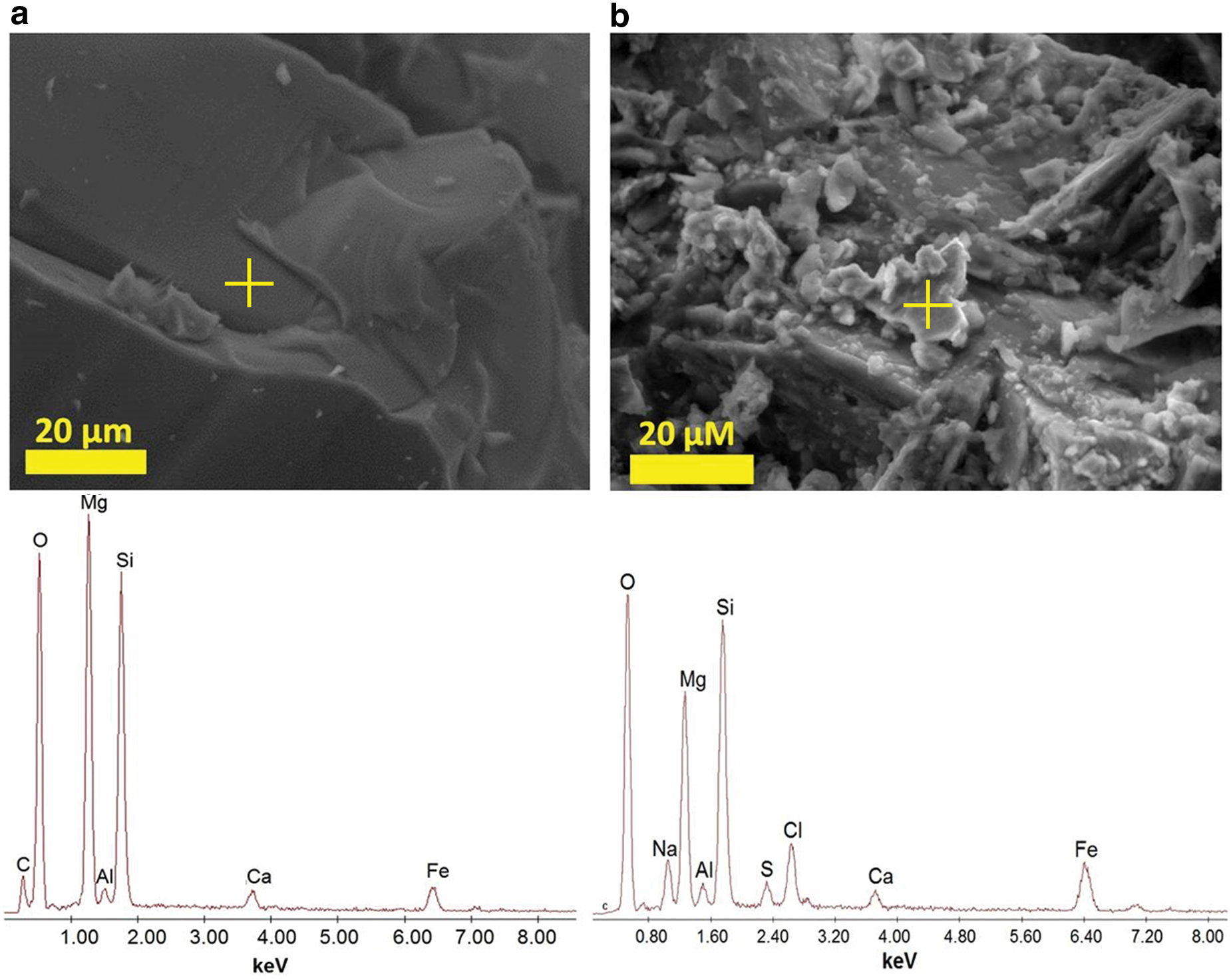
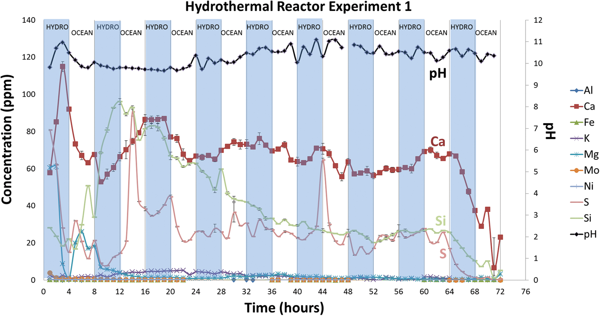
Environmental scanning electron microscope images and energy-dispersive spectrometer spectra collected from pre- (a) and postexperiment (b) reactor bed materials. Elemental analysis of Experiment 3 samples after the experiments reveals forsterite composition depleted in Mg (b) relative to starting compositions (a). Color images are available online.

FIG. 6.

Dissolved ion species and pH of solutions measured in the hydrothermal reactor control experiment with no CO₂. The shaded areas indicate hydrothermal fluid flow, and the nonshaded areas indicate ocean simulant flow. Color images are available online.

FIG. 7.

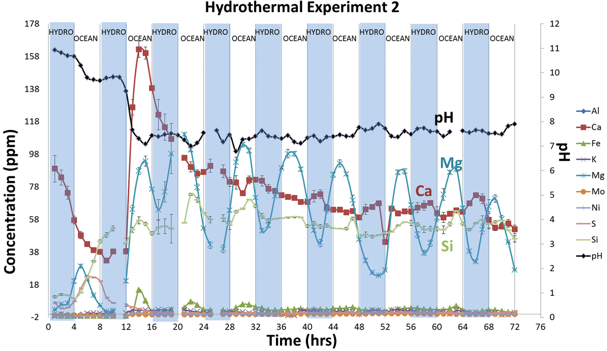
Dissolved ion species and pH of solutions collected hourly during hydrothermal reactor experiment with 10 bars of CO₂. The shaded areas indicate hydrothermal fluid flow, and the nonshaded areas indicate ocean simulant flow. Color images are available online.

In altered Experiment 3 materials, carbon abundances in 24 of the 121 ESEM/EDS spectra were as high as 24 atomic wt% (Supplementary Fig. S10). Similar carbon concentrations were observed in unaltered archean sulfides taken from the Timmins area, but in that case they were restricted to minerals rich in Mg, Ca, and O, interpreted from Raman analysis to be dolomite. Carbon mobilization is consistent with the generation of formate (section 4.4).

4.3. Dissolved inorganic detection

4.3.1. Experiment 1

Control experiment solutions showed high pH levels (pH ∼9–11) typical of alkaline hydrothermal fluids from the serpentinization of ultramafic rock (Fig. 6).

Solutions contained high concentrations of Ca, Mg, Si, and S during the initial 4 h of the experiments, during which it seems that these ions were flushed from the system. Ca reached a maximum of ∼115 ppm (2.87 mmol/kg) after 3 h of hydrothermal fluid flux, then dropped to ∼3 ppm (0.07 mmol/kg), fluctuating from 52 to 86 ppm (1.29–2.14 mmol/kg) until hour 19, when it stabilized around 63 ppm (1.57 mmol/kg) for the remainder of the experiment. Similarly, Mg, Si, and S fluctuated widely in the first ∼10 h of the experiment and equilibrated after ∼19 h. Mg levels peaked at ∼6 ppm (0.2 mmol/kg) after 6 h and dropped to zero after 13 h, as to be expected in the high pH solutions. Si levels reached a maximum of 96 ppm (3.4 mmol/kg) after 12 h and thereafter slowly dropped to near 30 ppm (1.0 mmol/kg). Sulfur reached a peak of 92 ppm (2.9 mmol/kg) at hour 14 and then fell after 16 h to near 25 ppm or 0.8 mmol/kg.

4.3.2. Experiment 2

This experiment showed a rapid drop in pH from 11 to between 7 and 8, as might be expected from interactions with the Hadean ocean simulant (Fig. 7) via mixing of pH ∼11 fluids with acidic ocean simulant (pH ∼5). Dissolved Mg concentrations contrasted with Experiment 1, oscillating with alterations of alkaline and carbonic fluid flow, presumably as the hydroxide dissolved in the acidic fluid. Following an early pulse, calcium concentrations dropped to ∼60 ppm and, finally, to around 50 ppm. Si followed a similar trend. Other compounds, including sulfur, were at or below the limits of detection (Fig. 7).

4.3.3. Experiment 3

Similar trends for Mg were observed in Experiment 3 as in Experiment 2. Mg levels rose ∼2 h after switching to ocean fluid flow, then dropped before switching back to hydrothermal fluid flow (Fig. 8). Sulfur correlates inversely with Mg, as expected from its solubility as the bisulfide (HS⁻). The highest S abundance (290 ppm; 9.0 mmol/kg) was measured at hour 10, ∼2 h after switching to hydrothermal fluid flow. Calcium levels were similar to those observed in Experiment 1, ranging from 27 to 86 ppm (0.7–2.2 mmol/kg) after the first 13 h. The highest Ca levels (129 ppm or 3.2 mmol/kg) were measured at the beginning of the experiment, leveling off at approximately hour 13—similar to trends observed in Experiments 1 and 2. Si concentrations for all solutions do not appear to correlate with the other solutes, nor can they be related to ocean or hydrothermal flow, remaining fairly steady throughout the entirety of the experiment between 15 and 42 ppm (0.5–1.5 mmol/kg).

FIG. 8.

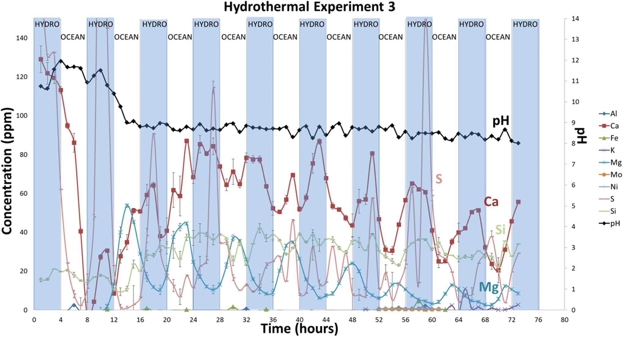
Dissolved ion species and pH of solutions collected every hour during hydrothermal reactor experiment with ∼1 bar CO₂. The shaded areas indicate hydrothermal fluid flow, and the nonshaded areas indicate when ocean simulant was flowing. Color images are available online.

4.4. Detection of formate and acetate

ICP-AES showed higher concentrations of aqueous Cl⁻ in Experiment 1 samples compared with Experiment 3. The close IEC peak centers for Cl⁻ (∼4.1 min) and the valeric acid internal standard (∼4.4 min) suggested coelution with the valeric acid internal standard, which prohibited the calculation of a dilution factor for the analyzed solutions. As a result, the concentrations of organic molecules could not be determined, but only their relative peak areas could be compared for trends, indicating the formation of formate or acetate. IEC analyses of samples from Experiment 2 solutions were close to detection limits.

Formate peak areas measured in Experiment 1 solutions were observed in a similar peak area range as those measured in Experiment 3. Yet, the trends observed for formate concentrations in Experiments 1 and 3 appear to be different. This implies minor generation or leaching of formate in Experiment 1, whereas in Experiment 3, the formate peaks correspond directly to the admission of CO₂-bearing ocean fluids (Fig. 9).

FIG. 9.

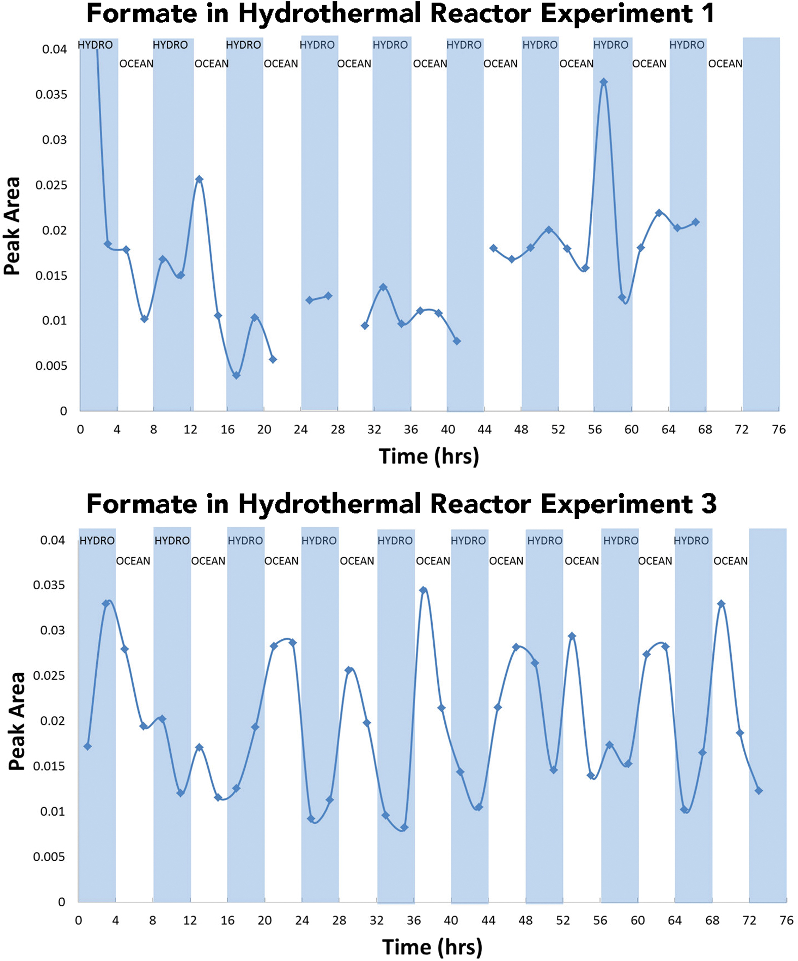
Formate peak areas measured from Experiment 1 solutions plotted versus time and solution type (top) compared with formate peak areas measured from Experiment 3 versus time and solution flow (bottom). Some data are missing from Experiment 1 results due to limited sample size. CO₂-rich ocean fluids cause a distinct trend, with spikes of formate in Experiment 3. By contrast, Experiment 1 concentrations do not appear to trend with fluid type. Color images are available online.

In the control experiment, the first two measurements of formate and acetate were elevated relative to other measurements (Fig. 9 and Supplementary Figure S11). We attribute this difference to error introduced by dilution. The original sample volumes were 0.4 mL for these two samples before desalting. Because 1.0 mL of these solutions was collected from desalting methods before IEC analysis, the samples had to be diluted before analysis. Thus, the measured abundances of formate and acetate in these samples may be close to the limits of detection.

In Experiment 3, formate and acetate were detected at concentrations as high as 13 and 20 μM, respectively (Supplementary Fig. S1). However, formate was detected during hours 0–4 before any ocean solution (CO₂) was introduced. After the first 4 h of the experiment, formate concentrations oscillated with the changing fluid sources. As might be predicted, formate peaked rapidly during oceanic fluid infusions, at ∼7 to 13 μM, and diminished during hydrothermal flow to lower levels (∼3 to 7 μM). The oscillation occurred at every fluid transition throughout the experiment, similar to the trend observed for dissolved Mg (Fig. 10).

FIG. 10.

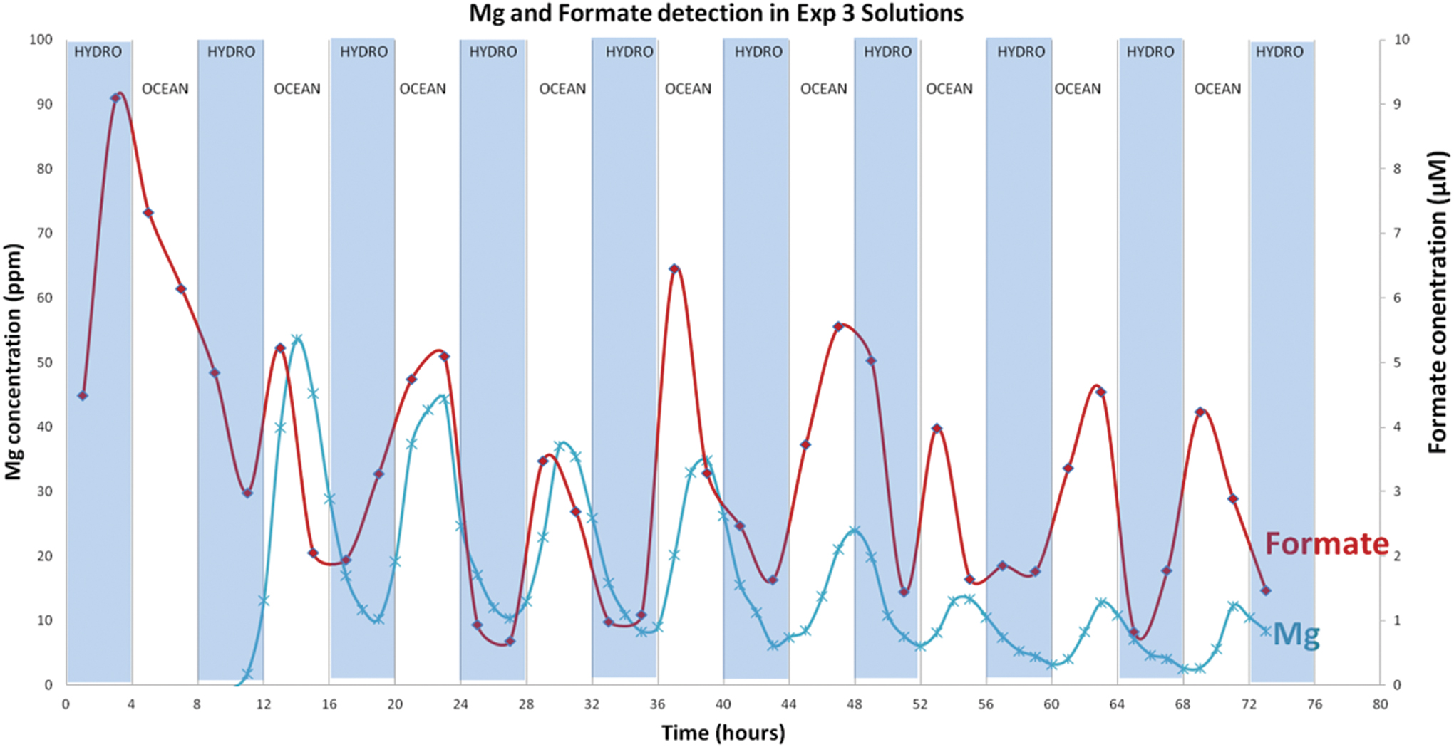
Comparison of measured Mg concentrations and measured formate concentrations in Experiment 3 solutions. Both follow a similar trend with ocean fluid flow indicating that partial serpentinization may be occurring while formate is being produced. The shaded areas indicate hydrothermal fluid flow, and the nonshaded areas indicate when ocean simulant was flowing. Hydrothermal and ocean simulated fluids were alternated every 4 h for the 72-h experiment. Color images are available online.

Acetate levels in Experiment 3, by contrast with formate, remained between 0 and 10 μM during the first 31 h of Experiment 3, rising to 15 μM at hour 33 and to 20 μM after ∼47 h, then dropping at hour ∼53 to the initial concentration of 0–10 μM (Supplementary Fig. S1). However, it cannot be ascertained from comparison of the raw peak areas from Experiment 1 solutions, whether abiotic acetate formed was generated from CO₂ or not.

4.5. Detection of methane

Methane concentrations were measured at 15-min intervals. Methane remained at a constant baseline around 30 ppb in control Experiment 1. Two spikes at ≤120 ppb, not shown, likely resulted from inadvertent leakage during insertion or removal of the sampling syringe (atmospheric CH₄, at ∼2 ppm, could not be ruled out). In Experiment 3, ¹³CH₄ remained at a baseline of around 10 ppb for the entire experiment. However, four spikes in labeled methane were observed between 50 and 80 ppb, which cannot be attributed to atmospheric leakage, as atmospheric ¹³CH₄ is at most ∼20 ppb (Fig. 11).

FIG. 11.

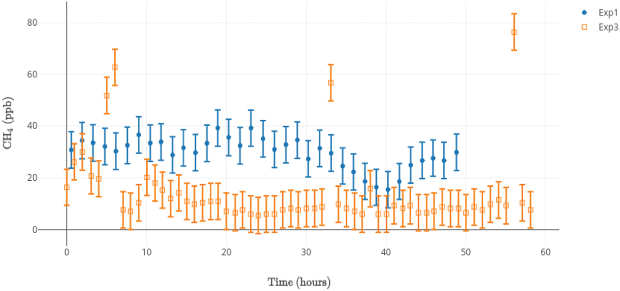
Methane ¹²CH₄ concentrations versus time for hydrothermal reactor Experiment 1 (blue, closed circles), and ¹³CH₄ concentrations versus time for hydrothermal reactor Experiment 3 (orange, open squares). There is no correlation between the carbonic inputs and the concentrations of CH₄. Observed ¹³CH₄ above the noise floor of ∼10 ppb cannot be attributed to atmospheric leakage, which would account for only ∼20 ppb. Such intermittent and uncorrelated bursts of methane of what must be the result of ¹³CO₂ reduction could be a result of sorption/desorption, bubble formation, and liberation and release (cf. Hu et al., 2016; Webster et al., 2018). Color images are available online.

5. Discussion

5.1. Solid reactor bed material analysis

Iron-bearing compounds were formed through simulated serpentinization in Experiments 1 and 3. Although dissolved Fe concentrations were close to zero in all experiments, hematite and mackinawite were observed only in altered solid samples. These results suggest dissolved iron was taken up in iron-bearing minerals or through the precipitation of iron sulfides, as observed in Experiments 1 and 3 materials. Iron sulfide minerals, including mackinawite, were confirmed by Raman analysis and could have resulted from iron and sulfur leaching (as Fe²⁺ and HS⁻) of reactor bed materials or through the alteration of pentlandite (Mielke et al., 2010). Pyrite, the oxidized end-member in the iron sulfide system (Harris and Nickel, 1972), was observed in Experiment 3. Although pyrite was not observed in the input pentlandite, it is often associated with pentlandite formation (Nickel et al., 1974). Thus, the presence of pyrite before the start of reactor experiments should not be discounted. Higher concentrations of sulfur and mackinawite in Experiment 1 relative to Experiments 2 and 3 suggest that the observed iron sulfides precipitated from solution, possibly nucleated on pyrrhotite grains (Cairns-Smith et al., 1992). The detection of iron sulfide mineral formation, including mackinawite and possibly pyrite, further supports the AHV theory in which iron sulfide catalysts, well known for enabling CO₂ reduction, could have been present in these ancient systems (White et al., 2015).

Silica abundances in each experiment—and relative to pre-experiment materials—were notably different. Silica was observed in most or all samples from Experiment 1, compared with Experiments 2 and 3 where silica was observed up to 24 and 40 volume% of the sample, repectively. In contrast, silica abundances in the input komatiite were below 10 volume%. Output solutions from Experiment 1 contained more dissolved Si (96 ppm) compared with Experiments 2 and 3 (∼60 and ∼40 ppm, respectively). Considering again that magnesium tends to dissolve during serpentinization of komatiite (reactions iii and iv), we infer that the process progresses given the release of Mg in Experiments 2 and 3, but that it reprecipitated, perhaps as brucite and/or carbonate. The elevated concentration of Si in Experiment 1 solutions, by contrast, indicates that dissolved silica from komatiite remained in solution, as might be expected of the elevated solubility of silica above pH 10 (Fleming and Crerar, 1982).

As Raman analysis showed no discernable hematite before alteration, its presence in the charges in all three experiments was unexpected. One possible explanation is that the mineral was present in unaltered bulk pentlandite samples below the 5 wt% threshold of the XRD and was nonhomogenously mixed such that it was not detectable by Raman analysis before alteration. Another possibility is that hematite was a product of olivine alteration, with the iron oxidation being coupled to the reduction of CO₂ to formate or even elemental carbon (Sforna et al., 2018; Peuble et al., 2019).

Another possible route is through oxidation of mackinawite while exposed to air during extraction of materials from the reactor bed before storage in N₂-purged vials. However, this seems unlikely given our previous work (White et al., 2015) where typical oxidation products of mackinawite in air or from beam effects during Raman analysis are magnetite and lepidocrocite.

5.2. Solution analyses

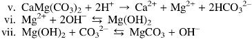
The CO₂ pressures in Experiments 1, 2, and 3 at 0, 10, and 1 bars, respectively, influenced the contents of the effluents. Experiment 3 fluids were less alkaline (pH 6–8) than those measured in Experiment 1 (pH 10–12). While the pH of the CO₂-absent fluids in Experiment 1 oscillated unevenly around 10 to 11 units, the addition of 1 and 10 bars of CO₂ to the ocean simulant in Experiments 3 and 2 dropped the pH to 8–9 and 7–8, respectively, after the first ∼14 h. Despite the fact that Experiment 1 ocean solution was titrated to pH ∼5, it appears the fluid interactions with ultramafic rock may be rapidly buffering the resulting solutions to an alkaline pH. This suggestion appears consistent with the occurrence of serpentinization, which would alter the solution to ∼pH 11 through dissolution of calcium and/or magnesium as hydroxide with the release of hydrogen. In contrast, the lower pH values observed in Experiments 2 and 3 could result from incomplete reaction of CO₂ in the solution with the starting materials (see reactions v–vii). Because extraction of reactor bed materials for analysis during the experiment was not possible, it is unclear if brucite (MgOH₂) was forming:

Solution analysis revealed trends in Mg and S with clear release of these ions along with Si as might be expected of partial serpentinization. We assume that the apparent absence of brucite in reactor materials suggests that Mg is continually redissolved (Ludwig et al., 2006). After flushing in the first 12 h, Mg values were negligible in the absence of CO₂ (Experiment 1), presumably because of the insolubility of brucite at high pH (reaction vi) (Palandri and Reed, 2004).

After the pH dropped in the other two experiments, Mg concentrations were strongly anticorrelated with the influx of CO₂-enriched waters, as observed in both Experiments 1 and 2 (Figs. 5 and 6).

The most noticeable difference in the ICP analyses of Experiment 3 solutions compared with Experiment 1 is the release of Mg, which rises when CO₂-rich ocean fluid is flowing and falls when alkaline hydrothermal solution is flowing. This Mg switching is consistent with the release of Mg from ultramafic rock during serpentinization upon reaction of alkaline fluids with komatiite. This can be understood by considering the serpentinization reaction (i) as three characteristic reactions (viii–x) (Bach et al., 2006; Frost and Beard, 2007; McCollom and Bach, 2009):

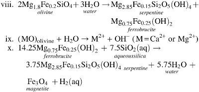
Reactions ix and x occur simultaneously and create an ∼pH 11 solution. In reaction ix, Mg²⁺ and Ca²⁺ are released as ocean waters interact with magnesium silicates (in this case forsterite, the Mg end member of olivine) before their transformation to serpentine. Magnesium is rendered more soluble during the exothermic serpentinization of olivine and pyroxene below 200°C (Macleod et al., 1994; Palandri and Reed, 2004). Therefore, the observed Mg release during ocean solution flow in Experiments 2 and 3 solutions may result through a similar reaction to reaction iii, where ocean water leaches Mg from forsterite before serpentine mineral formation. The higher abundance of silica observed in postexperiment materials (Fig. 10) further supports the interpretation that dissolution of komatiite is occurring. However, because no ferrobrucite or serpentine minerals were detected in postexperiment solid materials, serpentinization may only be incipient up to reaction xi. Alternatively, the reaction may have proceeded further, but the fine products were washed through. Since silica is soluble at pH >10, the release of the hydroxide ion tends to produce low-iron serpentine. The remaining iron is thus available for oxidation to magnetite (Supplementary Fig. S8), with the concomitant production of H₂(aq) (Frost and Beard, 2007; McCollom and Bach, 2009).

The sinusoidal pattern observed for dissolved Mg may be attributed to pH-induced precipitation and redissolution of Mg-bearing complexes. For example, once Mg is released from either carbonate or olivine source, it may react with alkaline fluids to form brucite [Mg(OH)₂] as part of the serpentinization and buffering reactions (viii and xi). However, once the tank solution is switched to ocean and acidic waters flow, the brucite redissolves, releasing Mg into solution. While Mg was released under these conditions, as we have noted, brucite was not detected by Raman analysis of postexperiment solids. Therefore, the precipitant formed during Mg fluxes remains unclear. However, dolomite was observed in postexperiment mineral analysis (Supplementary Figs. S5 and S8). The formation of dolomite could occur through reaction of dissolved carbon dioxide with dissolved Mg and Ca dissolved from the rocks introduced into the reactor and shown by ICP analysis to be present in reactor solutions. However, because the dolomite was also observed in pentlandites analyzed before the experiment (Table 2), its detection in postexperiment materials cannot be directly interpreted as being formed through the simulated serpentinization conditions.

Dissolved sulfur in the experimental solutions revealed anticorrelation with dissolved CO₂. In control Experiment 1, in the absence of CO₂, high but uneven abundances of sulfur (about 1 mmol/kg of the bisulfide HS⁻) were released throughout the duration of the experiment. This observation agrees with previous reactor experiments showing high sulfur abundances in alkaline hydrothermal reactor effluents (Mielke et al., 2010). This further supports the AHV theory, which assumes that Hadean submarine minerals produced from alkaline hydrothermal fluids derived from sulfide-bearing rocks would have included iron sulfides from the precipitation of bisulfide-rich effluents reacted with iron in acidic iron- and CO₂-rich ocean water. The mobilization of sulfur in the simulated Hadean system also supports the view that sulfur would have been present to a level of millimoles/kg in ancient alkaline serpentinizing solutions (Macleod et al., 1994). Prior experiments (White et al., 2015) mixing bisulfide-rich alkaline solutions with iron-rich acidic solutions at ∼75°C produced iron sulfides, including mackinawite and greigite. In contrast, in the presence of 1 bar CO₂ in Experiment 3, the sulfur content in the effluent was more uneven. As would be expected, spikes of sulfur were observed only during hydrothermal effluent flow and especially during the first ∼10 h of the experiment, that is, at more alkaline conditions.

5.3. Organic analyses

The consistent presence of methane (50–100 ppb) at levels well below typical methane concentrations in air (1800 ppb; Fig. 11) can be attributed to (1) introduction from ambient air, (2) production during the experiment, or (3) release from organic molecules bound in the mineral substrate charge (cf. Etiope et al., 2018). Considering the resulting ppb levels of methane detected in Experiment 1 (where no CO₂ was introduced), we conclude that significant quantities of methane did not form in the time frame of the hydrothermal simulations. The small quantities of labeled ¹³CH₄ in Experiment 3 may be attributed to intermittent occlusion in minerals comprising the reactor, and therefore, some CO₂ reduction. The spasmodic production may be understood from thermodynamic calculations permitting ¹³CH₄ production from ¹³CO₂ reduction within similar serpentinization conditions (Amend and McCollom, 2009), subject to the kinetics of the system that otherwise prevents significant reduction of CO₂ beyond formate (Schoonen et al., 1999).

Formate concentrations in Experiment 3 rose and fell with measured Mg concentrations, trending with the introduction of carbonic fluids. As magnesium is soluble below pH ∼10, these common trends suggest that a portion of the CO₂ was reduced to formate, and that the reduction was rapid (Figs. 10 and 11) (Frost and Beard, 2007). This interpretation is consistent with the mechanisms inferred for abiotic formate found at the Lost City hydrothermal field (Lang et al., 2010). However, formate may have been derived from multiple sources since it was detected during the first 4 h of the experiment, before any ocean solution (CO₂) was introduced, and presumably rapidly leached out from a primary source. Specifically, in addition to CO₂ reduction, formate could also be generated through alkaline fluid interaction with carbonates known to be present in reactor bed materials. Later, formate generation is likely to have resulted from hydrogen reacting with both carbonates in the reactor bed materials and CO₂ in the ocean solution. This would explain steadier oscillations in concentration after the first 4 h of the experiment.

In contrast to formate, no apparent trend was detected linking acetate concentrations to the alternating inputs of ocean and hydrothermal simulant. This leads us to the provisional assumption that the acetate resulted from contamination or organic breakdown. Similar uncertainties surround observations at Lost City by Lang et al. (2010; figure 3b), which led researchers there to infer a biological origin for the observed organic acid.

Our work supports the notion that kinetic barriers limit chemical reactions on the multiple-hour timescale of the experiments; CO₂-rich fluids did not interact with H₂-bearing fluids over catalysts in the reactor bed beyond the generation of formate excepting minor production of methane spasmodically released from occlusions. This finding comports with prior experiments (McCollom and Seewald, 2001; McDermott et al., 2015) and field observations (Kelley, 1996) suggesting that while CH₄ may be an important component of hydrothermal fluids, its formation by reducing CO₂ is sluggish. The interactions we simulated probably occur in nature over a broad range of longer path lengths and timescales. Peak serpentinization reactions in real hydrothermal systems take place at around 4 km depth below the ocean floor (P ∼ 100 MPa; Malvoisin et al., 2017), and they can proceed as deep as 12 to 15 km and, in the lower pressure environments of the icy ocean worlds, much deeper still (Shock, 1990; Russell et al., 1995; Schlindwein and Schmid, 2016; Vance et al., 2016; Waite et al., 2017). Since mackinawite was observed to form during these experiments, it could have aided in some catalytic reduction of CO₂ and perhaps the minimal amount of mackinawite formed explains apparent sporadic methane production. As suggested in our previous work (White et al., 2015), mackinawite and greigite are both predicted to comprise much of the ancient hydrothermal precipitates resulting from serpentinization reactions. Thus, the detection of some formate and spasmodic methane along with conversion of pentlandite to mackinawite supports the assumption that iron sulfide reactants would be available to catalyze organic synthesis (Muñoz-Santiburcio and Marx, 2017). This result also suggests that running reactions with a bulk composition of mackinawite and/or greigite would clarify their roles, if any, in CO₂—and whether such reductions could take place on even shorter timescales than those achieved here (72 h). It has also been suggested that methane production is sourced from carbon deep within the mantle, and even that dissolved formate and acetate are produced from reactions beginning with methane (Kelley et al., 2005). However, even at the high pressures and temperatures that likely obtained during the serpentinization reactions driving Lost City-type springs in the Hadean, methane is an unlikely product (McCollom and Seewald, 2001).

The initial reactions are kinetically and thermodynamically challenging, requiring coupling to exothermic reactions or steep gradients. The kinetic barrier is higher for methane synthesis because the addition of a hydride to a methyl group faces more of an obstacle than does the addition of a further carbon-bearing radical to the same group to produce H₃C-COO⁻ (Maden, 2000). Thus, a route to acetate seems more likely and closely resembles the acetyl coenzyme-A pathway that life can take, although our acetate results are inconclusive in this regard (cf. Russell and Martin, 2004; Muñoz-Velasco et al., 2018).

6. Conclusions

Experiments 2 and 3 were designed to simulate the geochemical conditions resulting from interaction of carbonic ocean with ultramafic Hadean crust during open-system hydrothermal convection at, and just below, the ocean floor, while Experient 1 was the control. Solid materials and the derived solutions showed some evidence of serpentinization and organic synthesis after subjecting the ultramafic ocean crust simulants to alternating hydrothermal and ocean fluids under submarine hydrothermal pressures (100 bar), temperatures (120°C), and pH conditions proposed to occur in ancient nonmagmatic hydrothermal systems. The most arresting result was the cyclic reduction of CO₂ to μM of formate, which was closely correlated with fluctuations in dissolved Mg (Fig. 10). This result suggests that the hard work of CO₂ reduction at the emergence of life may have been bypassed early on by this serpentinization reaction (Windman et al., 2007), that is, hydrothermal formate rather than CO₂ was one of the first feeds to an acetyl coenzyme-A pathway (Russell, 2018). The depletion of Mg and Si in the komatiite charge is consistent with such rapid reduction of CO₂ during serpentinization. However, reduction beyond formate to methane was limited and spasmodic as evidenced by the small sporadic records of ¹³CH₄ in Experiment 3 (Fig. 11). Indeed, the low but continuous records of CH₄ in the control Experiment 1 force the conclusion that the greater part of this reduced carbon is leached from the Hadean ultramafic/sulfide crustal simulant (Fig. 11). This sporadic generation of ¹³CH₄ at very low concentrations is consistent with recent findings that the abiotic contribution of methane venting from natural hydrothermal systems is minimal below 200°C (Wang et al., 2018), and that where it does occur in micromolar amounts, it is perhaps more likely derived from deeper sources than those operating during serpentinization and is merely leached or entrained in the convecting alkaline solutions (Figs. 1 and 11).

High sulfur concentrations, up to 9 mmol/kg of dissolved sulfide, demonstrated the propensity of these alkaline systems to offer bisulfide to the growing mounds (Macleod et al., 1994; Mielke et al., 2010; Meyer-Dombard and Amend, 2014). This is also indicated by the detection of mackinawite in altered reactor bed material. The detection of mackinawite further supports the notion that this known electron source, conductor, and catalyst for CO₂ reduction and organic molecule retention would have been present in ancient alkaline hydrothermal systems (Ferris et al., 1992; White et al., 2015; Yamaguchi et al., 2016; Muñoz-Santiburcio and Marx, 2017; Murugan et al., 2018).

Depleted Mg levels in ultramafic compositions compared with unaltered (pre-experiment) materials were consistent with the observed dissolution of silica from komatiite and its precipitation in solid samples at the distal end of the reactor where the pHs of the solutions were below those controlling silica solubility (Fleming and Crerar, 1982; Gourcerol et al., 2016). Although no serpentine minerals per se were identified in the postexperiment materials, the magnesium, calcium, and iron (in the alkaline solutions) correlated well with derived solutions that showed some evidence of serpentinization in the Lost City hydrothermal field and those intersected in drill holes into the magma-poor, passive Iberian margin (Klein et al., 2015).

The results of these experiments—in concert with other theoretical and experimental findings (Windman et al., 2007; McCollom and Donaldson, 2016; Russell and Nitschke, 2017)—demonstrate the utility of the protocols used in the operations of the JPL reactor instrument, as well as of the instrument itself, for simulating the nonequilibrium geochemical interactions feeding AHVs on ocean floors. Furthermore, results show that the JPL hydrothermal reactor can maintain far-from-equilibrium conditions up to 72 h to closely simulate the constant flux of a hydrothermal vent on both the water world that was the ancient Earth and on other planets and moons in the solar system and beyond (Vance et al., 2007; Hand et al., 2009; Etiope et al., 2013a; Russell et al., 2014; Glein et al., 2015; Hsu et al., 2015; Sekine et al., 2015; Shibuya et al., 2015; Vance et al., 2016; Choblet et al., 2017; Russell et al., 2017; Waite et al., 2017; Glein et al., 2018).

Footnotes

Acknowledgments

We thank the members of the Keck Institute for Space Studies workshop, Methane on Mars, for discussions. The sulfide samples were collected during a field expedition generously supported by the Agouron Institute. We thank Bill Warner and Mark Anderson of the JPL Analytical Chemistry Laboratory for IEC analysis of samples, Peter Willis, Amanda Stockton, and Morgan Cable for contributing to organic analysis of hydrothermal samples. Copyright 2018. All rights reserved before publication.

Author Disclosure Statement

No competing financial interests exist.

Funding Information

The research reported here was supported by the National Aeronautics and Space Administration, through the NASA Astrobiology Institute (NAI) under cooperative agreement issued through the Science Mission directorate; No. NNH13ZDA017C and 13-13NAI7_2-0024 (Icy Worlds) at the Jet Propulsion Laboratory. SDV was also supported by NAI grant 17-NAI8_2-0017 (Hydrocarbon Worlds) during completion of the writing of this work. L.M.W. was supported by the NASA Harriet-Jenkins Fellowship program while conducting this work.

Abbreviations Used

References

Amend

J.P.

and McCollom

T.M.

(2009) Energetics of biomolecule synthesis on early Earth. In Chemical Evolution II: From Origins of Life to Modern Society, edited by Zaikowski

, Friedrich

J.M.

, and Seidel

S.R.

, American Chemical Society, Washington, DC; ACS symposium series 1025:63–94.

Amend

J.P.

and Shock

E.L.

(2001) Energetics of overall metabolic reactions of thermophilic and hyperthermophilic archaea and bacteria. FEMS Microbiol Rev, 25:175–243.

Amiguet

, Van De Moortèle

, Cordier

, Hilairet

, and Reynard

(2014) Deformation mechanisms and rheology of serpentines in experiments and in nature. Journal of Geophysical Research: Solid Earth, 119:4640–4655.

Artemieva

I.M.

and Thybo

(2013) EUNAseis: a seismic model for Moho and crustal structure in Europe, Greenland, and the North Atlantic Region. Tectonophysics, 609:97–153

Bach

, Paulick

, Garrido

C.J.

, Ildefonse

, Meurer

W.P.

, and Humphris

S.E.

(2006) Unraveling the sequence of serpentinization reactions: petrography, mineral chemistry, and petrophysics of serpentinites from MAR 15°N (ODP Leg 209, Site 1274). Geophysical Research Letters. 33.

Barge

L.M.

, Flores

, Baum

M.M.

, VanderVelde

D.G.

, and Russell

M.J.

(2019) Redox and pH gradients drive amino acid synthesis in iron oxyhydroxide mineral systems. Proceedings of the National Academy of Sciences, page. 201812098.

Barnes

S.J.

and Fiorentini

M.L.

(2012) Komatiite magmas and sulfide nickel deposits: a comparison of variably endowed Archean terranes. Econ Geol, 107:755–780.

Bédard

J.H.

(2006) A catalytic delamination-driven model for coupled genesis of Archaean crust and sub-continental lithospheric mantle. Geochim Cosmochim Acta, 70:1188–1214.

Bethke

C.M.

(2007) Geochemical and Biogeochemical Reaction Modeling. Cambridge University Press, Cambridge UK.

10.

Branscomb

and Russell

M.J.

(2018) Frankenstein or a submarine alkaline vent: who is responsible for abiogenesis? Part 2: as life is now, so it must have been in the beginning. BioEssays, 40:1700182.

11.

Branscomb

, Biancalani

E.T.

, Goldenfeld

, and Russell

M.J.

(2017) Escapement mechanisms and the conversion of disequilibria: the engines of creation. Phys Rep, 677:1–6.

12.

Cairns-Smith

A.G.

, Hall

A.J.

, and Russell

M.J.

(1992) Mineral theories of the oirgin of life and an iron sulfide example. Orig Life Evol Biosph, 22:161–1380.

13.

Cann

J.R.

, Strens

M.R.

, and Rice

(1985) A simple magma-driven thermal balance model for the formation of volcanogenic massive sulphides. Earth Planet Sci Lett, 76:123–134.

14.

Choblet

, Tobie

, Sotin

, Běhounková

, Cădek

, Postberg

, and Souček

(2017) Powering prolonged hydrothermal activity inside enceladus. Nat Astron, 1:841–847.

15.

Christensen

L.E.

, Mansour

, and Yang

R.Q.

(2010) Thermoelectrically cooled interband cascade laser for field measurements. Opt Eng, 49:111119.

16.

Corliss

J.B.

, Baross

J.A.

, and Hoffman

S.E.

(1981) An hypothesis concerning the relationships between submarine hot springs and the origin of life on earth. Oceanologica Acta, 4(suppl):59–69.

17.

Cottrell

(1979) The natural philosophy of engines. Contemp Phys, 20:1–10.

18.

Downs

R.T.

(2006) The RRUFF project: an integrated study of the chemistry, crystallography, Raman and infrared spectroscopy of minerals. In: Program and Abstracts of the 19th General Meeting of the International Mineralogical Association in Kobe, Japan, pp O03–O13.

19.

Emmanuel

and Berkowitz

(2006) Suppression and stimulation of seafloor hydrothermal convection by exothermic mineral hydration. Earth Planet Sci Lett, 243:657–668.

20.

Etiope

and Ionescu

(2015) Low-temperature catalytic CO₂ hydrogenation with geological quantities of ruthenium: a possible abiotic CH₄ source in chromitite-rich serpentinized rocks. Geofluids, 15:438–452.

21.

Etiope

, Ehlmann

B.L.

, and Schoell

(2013a) Low temperature production and exhalation of methane from serpentinized rocks on Earth: a potential analog for methane production on Mars. Icarus, 224:276–285.

22.

Etiope

, Vance

, Christensen

, Marques

, and Ribeiro da Costa

(2013b) Methane in serpentinized ultramafic rocks in mainland Portugal. Mar Pet Geol, 45:12–16.

23.

Etiope

, Ifandi

, Nazzari

, Procesi

, Tsikouras

, Ventura

, Steele

, Tardini

, and Szatmari

(2018) Widespread abiotic methane in chromitites. Sci Rep, 8:8728.

24.

Ferris

F.G.

, Jack

T.R.

, and Bramhill

B.J.

(1992) Corrosion products associated with attached bacteria at an oil field water injection plant. Can J Microbiol, 38:1320–1324.

25.

Fleming

and Crerar

(1982) Silicic acid ionization and calculation of silica solubility at elevated temperature and pH application to geothermal fluid processing and reinjection. Geothermics, 11:15–29.

26.

Frost

B.R.

and Beard

J.S.

(2007) On silica activity and serpentinization. J Petrol, 48:1351–1368.

27.

Gäb

, Ballhaus

, Siemens

, Heuser

, Lissner

, Geisler

, and Garbe-Schönberg

(2017) Siderite cannot be used as CO₂ sensor for Archaean atmospheres. Geochim Cosmochim Acta, 214:209–225.

28.

Glein

C.R.

, Baross

J.A.

, and Waite

J.H.

(2015) The pH of Enceladus' ocean. Geochim Cosmochim Acta, 162:202–219.

29.

Glein

C.R.

, Postberg

, and Vance

S.D.

(2018) The geochemistry of Enceladus: composition and controls. In Enceladus and the Icy Moons of Saturn, edited by Schenk

P.M.

, Clark

R.N.

, C.J.A. Howett, Verbiscer

A.J.

, and Waite

J.H.

, Unoversity of Arizona Press, Tucson, AZ, pp 39–56.

30.

Gourcerol

, Thurston

, Kontak

, Côté-Mantha

, and Biczok

(2016) Depositional setting of Algoma-type banded iron formation. Precambrian Res, 281:47–79.

31.

Halevy

, Alesker

, Schuster

E.M.

, Popovitz-Biro

, and Feldman

(2017) A key role for green rust in the Precambrian oceans and the genesis of iron formations: Nat Geosci, 10:135–139,

32.

Hand

, Chyba

, Priscu

, Carlson

, and Nealson

(2009) Astrobiology and the potential for life on Europa. In Europa edited by R. T. Pappalardo, W. B. McKinnon, and K. Khurana, University of Arizona Press, Tucson, AZ, pp 589–629.

33.

Harris

D.C.

and Nickel

E.H.

(1972) Pentlandite compositions and associations in some mineral deposits. Can Mineral, 11:861–878.

34.

Hekinian

, Fevrier

, Bischoff

, Picot

, and Shanks

(1980) Sulfide deposits from the East Pacific Rise near 21 N. Science, 207:1433–1444.

35.

Herschy

, Whicher

, Camprubi

, Watson

, Dartnell

, Ward

, Evans

J.R.G.

, and Lane

(2014) An origin-of-life reactor to simulate alkaline hydrothermal vents. J Mol Evol, 79:213–227.

36.

Horita

and Berndt

M.E.

(1999) Abiogenic methane formation and isotopic fractionation under hydrothermal conditions. Science, 285:1055–1057.

37.

Hsu

H.-W.

, Postberg

, Sekine

, Shibuya

, Kempf

, Horányi

, Juhász

, Altobelli

, Suzuki

, and Masaki

(2015) Ongoing hydrothermal activities within Enceladus. Nature, 519:207–210.

38.

, Bloom

A.A.

, Gao

, Miller

C.E.

, and Yung

Y.L.

(2016) Hypotheses for near-surface exchange of methane on Mars. Astrobiology, 16:539–550.

39.

Jian

, Chen

Y.J.

, Singh

S.C.

, Li

, Zhao

, Ruan

, and Qiu

(2017) Seismic structure and magmatic construction of crust at the ultraslow-spreading Southwest Indian Ridge at 50° 28′E. J Geophys Res Solid Earth, 122:18–42.

40.

Kelley

D.S.

(1996) Methane-rich fluids in the oceanic crust. J Geophys Res Solid Earth, 101:2943–2962.

41.

Kelley

D.S.

, Karson

J.A.

, Blackman

D.K.

, Fruh-Green

G.L.

, Butterfield

D.A.

, Lilley

M.D.

, Olson

E.J.

, Schrenk

M.O.

, Roe

K.K.

, Lebon

G.T.

, and Rivizzigno

.; AT3-60 Shipboard Party. (2001) An off-axis hydrothermal vent field near the Mid-Atlantic Ridge at 30 degrees N. Nature, 412:145–149.

42.

Kelley

D.S.

, Karson

J.A.

, Früh-Green

G.L.

, Yoerger

D.R.

, Shank

T.M.

, Butterfield

D.A.

, Hayes

J.M.

, Schrenk

M.O.

, Olson

E.J.

, Proskurowski

, Jakuba

, Bradley

, Larson

, Ludwig

, Glickson

, Buckman

, Bradley

A.S.

, Brazelton

W.J.

, Roe

, Elend

M.J.

, Delacour

, Bernasconi

S.M.

, Lilley

M.D.

, Baross

J.A.

, Summons

R.T.

, and Sylva

S.P.

(2005) A serpentinite-hosted ecosystem: The Lost City hydrothermal field. Science, 307:1428–1434.

43.

Klein

, Humphris

S.E.

, Guo

, Schubotz

, Schwarzenbach

E.M.

, and Orsi

W.D.

(2015) Fluid mixing and the deep biosphere of a fossil Lost City-type hydrothermal system at the Iberia Margin. Proc Natl Acad Sci U S A, 112:12036–12041.

44.

Kump

L.R.

and Seyfried

W.E.

(2005) Hydrothermal Fe fluxes during the Precambrian: effect of low oceanic sulfate concentrations and low hydrostatic pressure on the composition of black smokers. Earth Planet Sci Lett, 235:654–662.

45.

Kusakabe

, Tanyileke

G.Z.

, McCord

S.A.

, and Schladow

S.G.

(2000) Recent pH and CO₂ profiles at Lakes Nyos and Monoun, Cameroon: implications for the degassing strategy and its numerical simulation. J Volcanol Geoth Res, 97:241–260.

46.

Lane

(2010) Chance or necessity? Bioenergetics and the probability of life. J Cosmol, 10:3286–3304.

47.

Lang

S.Q.

, Butterfield

D.A.

, Schulte

, Kelley

D.S.

, and Lilley

M.D.

(2010) Elevated concentrations of formate, acetate and dissolved organic carbon found at the Lost City hydrothermal field. Geochim Cosmochim Acta, 74:941–952.

48.

Lang

S.Q.

, Früh-Green

G.L.

, Bernasconi

S.M.

, Lilley

M.D.

, Proskurowski

, Méhay

, and Butterfield

D.A.

(2012) Microbial utilization of abiogenic carbon and hydrogen in a serpentinite-hosted system. Geochim Cosmochim Acta, 92:82–99.

49.

Lang

S.Q.

, Früh-Green

G.L.

, Bernasconi

S.M.

, Brazelton

W.J.

, Schrenk

M.O.

, and McGonigle

J.M.

(2018) Deeply-sourced formate fuels sulfate reducers but not methanogens at Lost City hydrothermal field. Sci Rep, 8:755.

50.

Lowell

R.P.

and Rona

P.A.

(2002) Seafloor hydrothermal systems driven by serpentinization of peridotite. Geophys Res Lett, 29:26-1–26-4.

51.

Ludwig

K.A.

, Kelley

D.S.

, Butterfield

D.A.

, Nelson

B.K.

, and Früh-Green

(2006) Formation and evolution of carbonate chimneys at the Lost City hydrothermal field. Geochim Cosmochim Acta, 70:3625–3645.

52.

Macleod

, McKeown

, Hall

A.J.

, and Russell

M.J.

(1994) Hydrothermal and oceanic pH conditions of possible relevance to the origin of life. Orig Life Evol Biosph, 24:19–41.

53.

Maden

B.E.H.

(2000) Tetrahydrofolate and tetrahydromethanopterin compared: functionally distinct carriers in C-1 metabolism. Biochem J, 350:609–629.

54.

Malvoisin

, Brantut

, and Kaczmarek

M.A.

(2017) Control of serpentinisation rate by reaction-induced cracking. Earth Planet Sci Lett, 476:143–152.

55.

Martin

and Russell

M.J.

(2007) On the origin of biochemistry at an alkaline hydrothermal vent. Philos Trans R Soc Lond B Biol Sci, 362:1887–1926.

56.

McCollom

T.M.

and Bach

(2009) Thermodynamic constraints on hydrogen generation during serpentinization of ultramafic rocks. Geochim Cosmochim Acta, 73:856–875.

57.

McCollom

T.M.

and Donaldson

(2016) Generation of hydrogen and methane during experimental low-temperature reaction of ultramafic rocks with water. Astrobiology, 16:389–406.

58.

McCollom

T.M.

, and Seewald

J.S.

(2001) A reassessment of the potential for reduction of dissolved CO₂ to hydrocarbons during serpentinization of olivine. Geochim Cosmochim Acta, 65:3769–3778.

59.

McCollom

T.M.

, and Seewald

J.S.

(2003) Experimental constraints on the hydrothermal reactivity of organic acids and acid anions: I. Formic acid and formate. Geochim Cosmochim Acta, 67:3625–3644.

60.

McDermott

J.M.

, Seewald

J.S.

, German

C.R.

, and Sylva

S.P.

(2015) Pathways for abiotic organic synthesis at submarine hydrothermal fields. Proc Natl Acad Sci U S A, 112:7668–7672.

61.

McGlynn

S.E.

, Mulder

D.W.

, Shepard

E.M.

, Broderick

J.B.

, and Peters

J.W.

(2009) Hydrogenase cluster biosynthesis: organometallic chemistry nature's way. Dalton Trans, 22:4274–4285.

62.

Meyer-Dombard

D.R.

and Amend

J.P.

(2014) Geochemistry and microbial ecology in alkaline hot springs of Ambitle Island, Papua New Guinea. Extremophiles, 18:763–778.

63.

Mielke

R.E.

, Russell

M.J.

, Wilson

P.R.

, McGlynn

S.E.

, Coleman

, Kidd

, and Kanik

(2010) Design, fabrication, and test of a hydrothermal reactor for origin-of-life experiments. Astrobiology, 10:799–810.

64.

Mielke

R.E.

, Robinson

K.J.

, White

L.M.

, McGlynn

S.E.

, McEachern

, Bhartia

, Kanik

, and Russell

M.J.

(2011) Iron-sulfide-bearing chimneys as potential catalytic energy traps at life's emergence. Astrobiology, 11:933–950.

65.

Miller

S.L.

and Bada

J.L.

(1988) Submarine hot springs and the origin of life. Nature, 334:609–611.

66.

Moore

W.B.

and Webb

A.G.

(2013) Heat-pipe Earth. Nature, 501:501–505.

67.

Muñoz-Santiburcio

and Marx

(2017) Chemistry in nanoconfined water. Chem Sci, 8:3444–3452.

68.

Muñoz-Velasco

, García-Ferris

, Hernandez-Morales

, Lazcano

, Peretó

, and Becerra

(2018) Methanogenesis on early stages of life: ancient but not primordial. Orig Life Evol Biosph, 48:407–420.

69.

Murugan

, Miran

, Masuda

, Lee

D.S.

, and Okamoto

(2018) Biosynthesized iron sulfide nanocluster enhanced anodic current generation by sulfate reducing bacteria in microbial fuel cells. ChemElectroChem, 5:4015–4020.

70.

Neal

and Stanger

(1984) Calcium and magnesium hydroxide precipitation from alkaline groundwater in Oman, and their significance to the process of serpentinization. Mineralogical Magazine, 48:237–241.

71.

Neubeck

, Duc

, Bastviken

, Crill

, and Holm

N.G.

(2011) Formation of H₂ and CH₄ by weathering of olivine at temperatures between 30 and 70°C. Geochem Trans, 12:6.

72.

Nickel

E.H.

, Ross

J.R.

, and Thornber

M. R.

(1974) Supergene alteration of pyrrhotite-pentlandite ore at Kamblada, Western-Australia. Econ Geol, 69:93–107.

73.

Olive

J.A.

and Crone

T.J.

(2018) Smoke without fire: how long can thermal cracking sustain hydrothermal circulation in the absence of magmatic heat?. J Geophys Res Solid Earth, 123:4561–4581.

74.

Palandri

J.L.

and Reed

M.H.

(2004) Geochemical models of metasomatism in ultramafic systems: serpentinization, rodingitization, and sea floor carbonate chimney precipitation. Geochim Cosmochim Acta, 68:1115–1133.

75.

Pisapia

, Gérard

, Lecourt

, Lang

S.Q.

, Pelletier

, Payri

C.E.

, Monnin

, Guentas

, Postec

, and Quéméneur

(2017) Mineralizing filamentous bacteria from the Prony Bay Hydrothermal Field give new insights into the functioning of serpentinization-based subseafloor ecosystems. Front Microbiol, 8:57.

76.

Price

, Boyd

E.S.

, Hoehler

T.M.

, Wehrmann

L.M.

, Bogason

, Valtýsson

.þ., Örlygsson

, Gautason

, and Amend

J.P.

(2017) Alkaline vents and steep Na⁺ gradients from ridge-flank basalts—implications for the origin and evolution of life. Geology, 45:1135–1138.

77.

Proskurowski

, Lilley

M.D.

, Kelley

D.S.

, and Olson

E.J.

(2006) Low temperature volatile production at the Lost City Hydrothermal Field, evidence from a hydrogen stable isotope geothermometer. Chemical Geology, 229:331–343.

78.

Proskurowski

, Lilley

M.D.

, Seewald

J.S.

, Früh-Green

G.L.

, Olson

E.J.

, Lupton

J.E.

, Sylva

S.P.

, and Kelley

D.S.

(2008) Abiogenic hydrocarbon production at Lost City hydrothermal field. Science, 319:604–607.

79.

Peuble

, Godard

, Gouze

, Leprovost

, Martinez

, and Shilobreeva

(2019) Control of CO2 on flow and reaction paths in olivine-dominated basements: An experimental study. Geochimica et Cosmochimica Acta, 252:16–38.

80.

Reeves

E.P.

, McDermott

J.M.

, and Seewald

J.S.

(2014) The origin of methanethiol in midocean ridge hydrothermal fluids. Proc Natl Acad Sci U S A, 111:5474–5479.

81.

Russell

M.J.

(2003). The importance of being alkaline. Science, 302:580–581.

82.

Russell

M.J.

(2018) Green rust: the organizing seed of all life?. Life, 8:35.

83.

Russell

M.J.

and Hall

A.J.

(1997) The emergence of life from iron monosulphide bubbles at a submarine hydrothermal redox and pH front. J Geol Soc, 154:377–402.

84.

Russell

M.J.

and Hall

A.J.

(2006) The onset and early evolution of life. Geol Soc Am, 198:1–32.

85.

Russell

M.J.

and Martin

(2004) The rocky roots of the acetyl-CoA pathway. Trends Biochem Sci, 29:358–363.

86.

Russell

M.J.

and Nitschke

(2017) Methane: fuel or exhaust at the emergence of life?. Astrobiology, 17:1053–1066.

87.

Russell

M.J.

, Hall

A.J.

, and Turner

(1989) In vitro growth of iron sulphide chimneys: possible culture chambers for origin-of-life experiments. Terra Nova, 1:238–241.

88.

Russell

M.J.

, Couples

G.D.

, and Lewis

(1995) SEDEX genesis and super-deep boreholes: can hydrostatic pore pressures exist down to the brittle-ductile boundary. In Mineral Deposits: From Their Origin to Their Environmental Impact, ed. J. Pasava, B. Kribek, and K. Zak. CRC Press, Balkema, Rotterdam, pp 315–318.

89.

Russell

M.J.

, Hall

A.J.

, and Martin

(2010) Serpentinization as a source of energy at the origin of life. Geobiology, 8:355–371.

90.

Russell

M.J.

, Barge

L.M.

, Bhartia

, Bocanegra

, Bracher

P.J.

, Branscomb

, Kidd

, McGlynn

, Meier

D. H.

, Nitschke

, Shibuya

, Vance

, White

, and Kanik

(2014) The drive to life on wet and icy worlds. Astrobiology, 14:308–343.

91.

Russell

M.J.

, Murray

A.E.

, and Hand

K.P.

(2017) The possible emergence of life and differentiation of a shallow biosphere on irradiated icy worlds: the example of Europa. Astrobiology, 17:1265–1273.

92.

Salthammer

(2013) Formaldehyde in the ambient atmosphere: from an indoor pollutant to an outdoor pollutant?. Angew Chem Int Edit, 52:3320–3327.

93.

Schlindwein

and Schmid

(2016) Mid-ocean-ridge seismicity reveals extreme types of ocean lithosphere. Nature, 535:276–279.

94.

Schoonen

M.A.

A, Xu

, and Bebie

(1999) Energetics and kinetics of the prebiotic synthesis of simple organic acids and amino acids with the FeS-H₂S/FeS₂ redox couple as reductant. Orig Life Evol Biosph, 29:5–32.

95.

Seewald

J.S.

, Zolotov

M.Y.

, and McCollom

(2006) Experimental investigation of single carbon compounds under hydrothermal conditions. Geochim Cosmochim Acta, 70:446–460.

96.

Sekine

, Shibuya

, Postberg

, Hsu

H.-W.

, Suzuki

, Masaki

, Kuwatani

, Mori

, Hong

P.K.

, Yoshizaki

, Tachibana

, and Sirono

(2015) High-temperature water-rock interactions and hydrothermal environments in the chondrite-like core of Enceladus. Nat Commun, 6:8604.

97.

Sforna

M.C.

, Brunelli

, Pisapia

, Pasini

, Malferrari

, and Ménez

(2018) Abiotic formation of condensed carbonaceous matter in the hydrating oceanic crust. Nat Commun, 9:5049.

98.

Shanks

III

, W.C.P. and Thurston

, editors. (2012) Volcanogenic Massive Sulfide Occurrence Model. US Geological Survey Scientific Investigations Report 2010–5070–C, 345 pp. Reston, VA, USA.

99.

Shibuya

, Komiya

, Nakamura

, Takai

, and Maruyama

(2010) Highly alkaline, high-temperature hydrothermal fluids in the early Archean ocean. Precambrian Res, 182:230–238.

100.

Shibuya

, Yoshizaki

, Sato

, Shimizu

, Nakamura

, Omori

, Suzuki

, Takai

, Tsunakawa

, and Maruyama

(2015) Hydrogen-rich hydrothermal environments in the Hadean ocean inferred from serpentinization of komatiites at 300°C and 500 bar. Prog Earth Planet Sci, 2:246.

101.

Shibuya

, Russell

M.J.

, and Takai

(2016) Free energy distribution and hydrothermal mineral precipitation in Hadean submarine alkaline vent systems: importance of iron redox reactions under anoxic conditions. Geochim Cosmochim Acta, 175:1–19.

102.

Shock

E.L.

(1990) Geochemical constraints on the origin of organic-compounds in hydrothermal systems. Orig Life Evol Biosph, 20:331–367.

103.

Shock

E.L.

(1992) Chemical environments of submarine hydrothermal systems. Orig Life Evol Biosph, 22:67–107.

104.

Spiess

, Macdonald

K.C.

, Atwater

, Bal

, Francheteau

, Guerrero

, Hawkins

, Hayi

, Hessler

, and Juteau

M.K.

(1980) East Pacific Rise: hot springs and geophysical experiments. Science, 207:28.

105.

Suda

, Ueno

, Yoshizaki

, Nakamura

, Kurokawa

, Nishiyama

, Yoshino

, Hongoh

, and Kawachi

(2014) Origin of methane in serpentinite-hosted hydrothermal systems: the CH₄–H₂–H₂O hydrogen isotope systematics of the Hakuba Happo hot spring. Earth Planet Sci Lett, 386:112–125.

106.

Thomson

J.E.

, Ferguson

S.A.

, Johnston

W.G.Q.

, Pye

E.G.

, Savage

W.S.

, and Thomson

(1957) Copper, nickel, lead and zinc deposits in Ontario. Metal Resources Circular No. 2 of the Ontario Department of Mines, Toronto: Province of Ontario, Dept. of Mines.

107.

Tosca

N.J.

, Guggenheim

, and Pufahl

P.K.

(2016) An authigenic origin for Precambrian greenalite: implications for iron formation and the chemistry of ancient seawater. Geol Soc Am Bull, 128:511–530.

108.

Ueda

, Shibuya

, Sawaki

, Saitoh

, Takai

, and Maruyama

(2016) Reactions between komatiite and CO₂-rich seawater at 250°C and 350°C, 500 bars: implications for hydrogen generation in the Hadean seafloor hydrothermal system. Prog Earth Planet Sci, 3:35.

109.

Vance

, Harnmeijer

, Kimura

, Hussmann

, Demartin

, and Brown

J.M.

(2007) Hydrothermal systems in small ocean planets. Astrobiology, 7:987–1005.

110.

Vance

, Hand

, and Pappalardo

(2016) Geophysical controls of chemical disequilibria in Europa. Geophys Res Lett, 43:4871–4879.

111.

Waite

J.H.

, Glein

C.R.

, Perryman

R.S.

, Teolis

B.D.

, Magee

B.A.

, Miller

, Grimes

, Perry

M.E.

, Miller

K.E.

, Bouquet

, Luninem

J.I.

, Brockwell

, and Bolton

S.J.

(2017) Cassini finds molecular hydrogen in the Enceladus plume: evidence for hydrothermal processes. Science, 356:155–159.

112.

Wang

D.T.

, Reeves

E.P.

, McDermott

J.M.

, Seewald

J.S.

, and Ono

(2018) Clumped isotopologue constraints on the origin of methane at seafloor hot springs. Geochim Cosmochim Acta, 223:141–158.

113.

Wang

, Barge

L. M.

, and Steinbock

(2019) Microfluidic production of pyrophosphate catalyzed by mineral membranes with steep pH gradients. Chemistry, 25:4732–4739.

114.

Webster

C.R.

and Mahaffy

P.R.

(2011) Determining the local abundance of Martian methane and its ¹³C/¹²C and D/H isotopic ratios for comparison with related gas and soil analysis on the 2011 Mars Science Laboratory (MSL) mission. Planet Space Sci, 59:271–283.

115.

Webster

C.R.

, Mahaffy

P.R.

, Atreya

S.K.

, Moores

J.E.

, Flesch

G.J.

, Malespin

, McKay

C.P.

, Martinez

, Smith

C.L.

, Martin-Torres

, and Gomez-Elvira

(2018) Background levels of methane in Mars' atmosphere show strong seasonal variations. Science, 360:1093–1096.

116.

Welhan

J.T.

and Craig

(1979) Methane and hydrogen in East Pacific Rise hydrothermal fluids. Geophys Res Lett, 6:829–831.

117.

Wetzel

L.R.

and Shock

E.L.

(2000) Distinguishing ultramafic- from basalt-hosted submarine hydrothermal systems by comparing calculated vent fluid compositions. J Geophys Res Solid Earth, 105:8319–8340.

118.

White

L.M.

, Bhartia

, Stucky

G. D.

, Kanik

, and Russell

M.J.

(2015) Mackinawite and greigite in ancient alkaline hydrothermal chimneys: identifying potential key catalysts for emergent life. Earth Planet Sci Lett, 430:105–114.

119.

Windman

, Zolotova

, Schwandner

, and Shock

E.L.

(2007) Formate as an energy source for microbial metabolism in chemosynthetic zones of hydrothermal ecosystems. Astrobiology, 7:873–890.

120.

Yamaguchi

, Li

, Takashima

, Hashimoto

, and Nakamura

(2016) CO₂ reduction using an electrochemical approach from chemical, biological, and geological aspects in the ancient and modern Earth. In Solar to Chemical Energy Conversion, Eds M. Sugiyama, K. Fujii, S. Nakamura, Springer, Cham, pp 213–228.

121.

Yoshizaki

, Shibuya

, Suzuki

, Shimizu

, Nakamura

, Takai

, Omori

, and Maruyama

(2009) H₂ generation by experimental hydrothermal alteration of komatiitic glass at 300 degrees C and 500 bars: a preliminary result from on-going experiment. Geochem J, 43:E17–E22.

Supplementary Material

Please find the following supplemental material available below.

For Open Access articles published under a Creative Commons License, all supplemental material carries the same license as the article it is associated with.

For non-Open Access articles published, all supplemental material carries a non-exclusive license, and permission requests for re-use of supplemental material or any part of supplemental material shall be sent directly to the copyright owner as specified in the copyright notice associated with the article.

0.00 MB

0.12 MB

0.17 MB

0.13 MB

0.20 MB

0.23 MB

0.22 MB

0.20 MB

0.13 MB

0.14 MB

0.21 MB

0.17 MB