
Abstract
The search for possible biosignature gases in habitable exoplanet atmospheres is accelerating, although actual observations are likely years away. This work adds isoprene, C5H8, to the roster of biosignature gases. We found that isoprene geochemical formation is highly thermodynamically disfavored and has no known abiotic false positives. The isoprene production rate on Earth rivals that of methane (CH4; ∼500 Tg/year). Unlike methane, on Earth isoprene is rapidly destroyed by oxygen-containing radicals. Although isoprene is predominantly produced by deciduous trees, isoprene production is ubiquitous to a diverse array of evolutionary distant organisms, from bacteria to plants and animals—few, if any, volatile secondary metabolites have a larger evolutionary reach. Although non-photochemical sinks of isoprene may exist, such as degradation of isoprene by life or other high deposition rates, destruction of isoprene in an anoxic atmosphere is mainly driven by photochemistry. Motivated by the concept that isoprene might accumulate in anoxic environments, we model the photochemistry and spectroscopic detection of isoprene in habitable temperature, rocky exoplanet anoxic atmospheres with a variety of atmosphere compositions under different host star ultraviolet fluxes. Limited by an assumed 10 ppm instrument noise floor, habitable atmosphere characterization when using James Webb Space Telescope (JWST) is only achievable with a transit signal similar or larger than that for a super-Earth-sized exoplanet transiting an M dwarf star with an H2-dominated atmosphere. Unfortunately, isoprene cannot accumulate to detectable abundance without entering a run-away phase, which occurs at a very high production rate, ∼100 times the Earth's production rate. In this run-away scenario, isoprene will accumulate to >100 ppm, and its spectral features are detectable with ∼20 JWST transits. One caveat is that some isoprene spectral features are hard to distinguish from those of methane and also from other hydrocarbons containing the isoprene substructure. Despite these challenges, isoprene is worth adding to the menu of potential biosignature gases.
1. Introduction
For 90
Beyond JWST, the large ground-based telescopes now under construction (Giant Magellan Telescope, Johns et al., 2012; Extremely Large Telescope, Skidmore et al., 2015; and Thirty Meter Telescope, Tamai and Spyromilio, 2014) are expected to come online in the coming decade, and with the right instrumentation are expected to be able to study rocky planets around M dwarf stars by direct imaging. ESA's Atmospheric Remote-sensing Infrared Exoplanet Large-survey (ARIEL) (Gardner et al., 2006; Pascale et al., 2018) is planned for launch in 2028 and may be able to reach down to observe transiting super-Earth-sized exoplanets around the smallest M dwarf stars. These facilities will provide an excellent opportunity to detect biosignature gases.
However, oxygen alone does not tell the full tale as life on the Earth produces thousands of gases other than oxygen. Some volatiles produced by life on the Earth, such as methane (CH4), and nitrous oxide (N2O) are prominent in the Earth's atmosphere and therefore have been studied in the context of exoplanet atmosphere biosignature gases. Other gases produced by life are present only as trace gases (<1 parts per billion by volume [ppbv]) in the Earth's atmosphere. The possibility that life elsewhere may generate gases different than gases produced by life on the Earth and in larger quantities has motivated studies of gases such as dimethyl sulfide (DMS), dimethyldisulfide (DMDS), methyl chloride (CH3Cl), and phosphine (PH3) (Pilcher, 2003; Segura et al., 2005; Domagal-Goldman et al., 2011; Sousa-Silva et al., 2020). For a review of exoplanet atmosphere biosignature gases, see the works of Grenfell (2018), Kiang et al. (2018), Schwieterman et al. (2018), and Seager et al. (2016).
In this work, we add isoprene (C5H8) (Fig. 1) to the list of biosignature gases to be considered for detection in future missions. Isoprene is a hydrocarbon containing two carbon–carbon double bonds connected by one carbon–carbon single bond, or a “conjugated diene.”

The chemical structure of isoprene. Carbon atoms are shown in dark gray, and hydrogen atoms are indicated in white. Isoprene (C5H8 or 2-methyl-1,3 butadiene) is a conjugated-diene with a methyl group attached to the second position. Conjugated dienes are two double bonds separated by one single bond. C5H8, isoprene.
Isoprene on the Earth is predominately produced by deciduous trees and land plants. The production rate of isoprene is about 500 Tg/year (Sharkey et al., 2008), which is comparable to the production rate of methane, also 500 Tg/year (e.g., Dlugokencky et al., 2011). For a more detailed decomposition of isoprene sources and sinks, see Fig. 2. To our knowledge, isoprene has not yet been evaluated in detail as an exoplanet biosignature gas (although it has been briefly mentioned in the works of Seager et al., 2012; Grenfell, 2017).

Schematic of the major sources and sinks of isoprene in the Earth's atmosphere. The isoprene sources (up arrows and green numbers) and sinks (down arrows and red values) are shown. The thickness of arrows provides a relative estimation of the contribution of various sources and sinks of isoprene (McGenity et al., 2018). Color images are available online.
On first consideration, one might disregard isoprene as a potential biosignature gas because of its short lifetime (<3 hours) in the Earth's atmosphere. The short lifetime results in a very low isoprene atmospheric abundance, ranging from 1 to 5 ppbv only in localized regions above cities and forests (Sharkey et al., 2008) to no detection above deserts. In the Earth's atmosphere, isoprene is primarily regarded as a precursor to secondary organic aerosols. This is because once isoprene is released into the atmosphere it is rapidly destroyed by reactions with ⋅OH, and subsequent reactions with O2, to form diverse and reactive products. The intermediate products subsequently react with a wide variety of atmospheric components, including trace gases, and NO3 − and Cl− radicals, eventually forming aerosols † (Fan and Zhang, 2004; Teng et al., 2017) (Fig. 3).
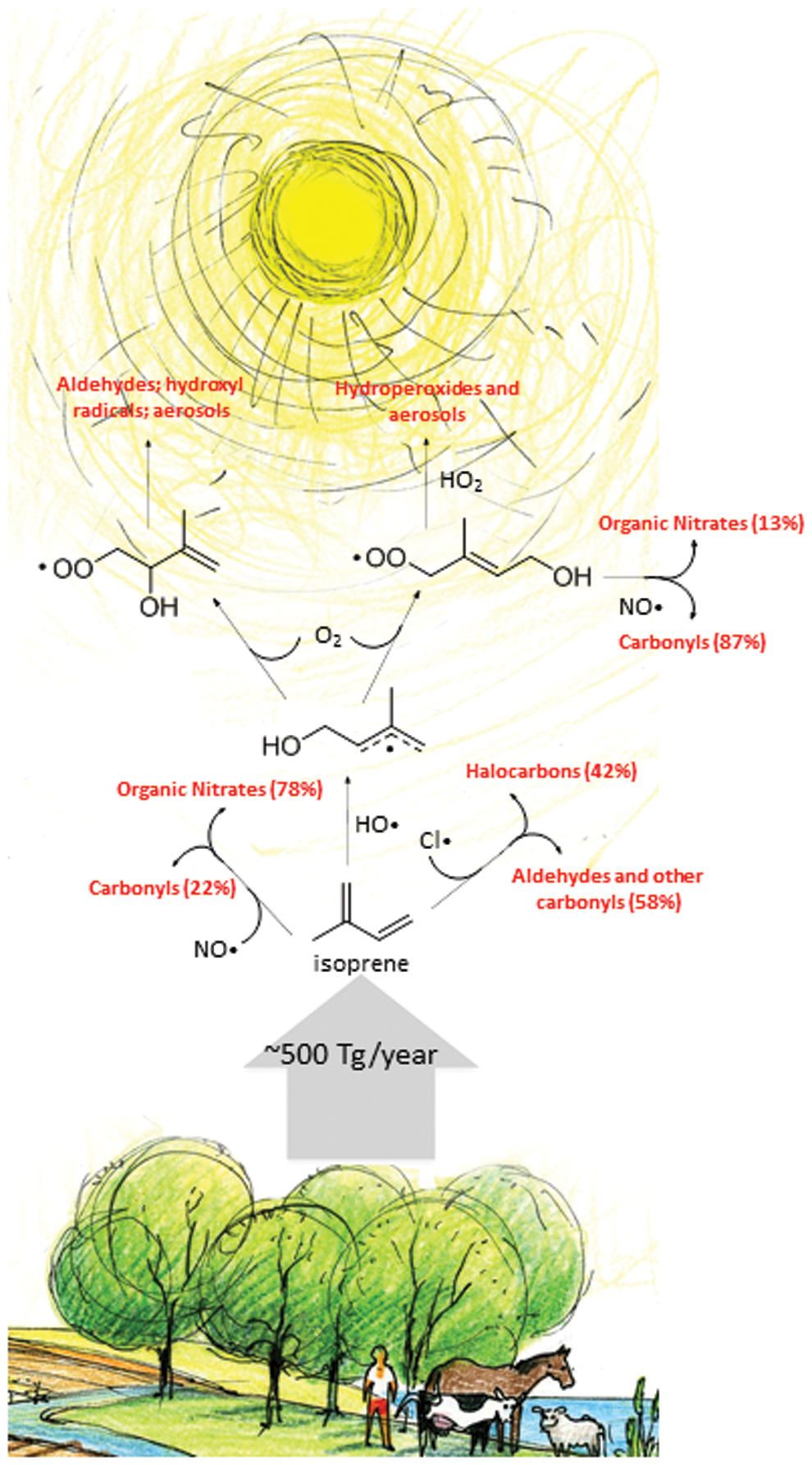
Schematic of the fate of the isoprene in the Earth's atmosphere. The oxidation of isoprene by OH radicals is the main pathway for the destruction of isoprene in the Earth's atmosphere (Teng et al., 2017). Less predominant destruction pathways include the reaction with NO• and Cl• radicals (Fan and Zhang, 2004). We note that the photochemically driven reactions with minor radical species (e.g., NO• species) can also proceed with downstream isoprene radical products (Iso[O2]); see, for example, Fan and Zhang (2004) for detailed pathways of photochemically driven atmospheric oxidation of isoprene species. Color images are available online.
However, the lack of OH− isoprene under anoxic conditions motivates its assessment as a biosignature gas. The Earth's atmosphere had no oxygen during its initial 2.4 Gyr and isoprene could, in principle, accumulate in anoxic atmospheres to detectable levels (Holland, 2006).
In this article, we evaluate isoprene as a biosignature gas. We first summarize isoprene's sources and sinks (Section 2), including isoprene's overall production on the Earth (Section 2.1), with details on isoprene's biological production from diverse organisms, both aerobic and anaerobic (Section 2.2), followed by a review of the known destruction mechanisms for isoprene (Section 2.3). Next, we outline our inputs and methods to assess the detectability of isoprene for a diverse set of anoxic atmosphere scenarios (Section 3). We discuss our main findings (Section 4): First, we present the production rates required for isoprene to accumulate to a detectable level in a given atmosphere scenario (Section 4.1); next, we assess whether isoprene can be detected by using JWST with a reasonable number of transit observations (Section 4.2); then, we show that isoprene is not produced thermodynamically in the atmosphere and therefore that isoprene as a biosignature gas has no false positives in habitable exoplanet atmospheres (Section 4.3). Finally, we conclude the article with a discussion of our results, limitations, and caveats (Section 5).
2. Isoprene Sources and Sinks
Before we study the detection of isoprene in an exoplanet atmosphere, we first explore how isoprene is created and destroyed. On the Earth, isoprene production is biological (Sections 2.1 and 2.2). We explore the destruction pathways of isoprene, which is mainly by direct photolysis and with OH radicals and O2 (Fig. 3).
2.1. Isoprene productions on Earth
Globally, life on the Earth produces 400–600 Tg/year of isoprene (Guenther et al., 2006, 2012; Arneth et al., 2008). The biological production rate of isoprene on Earth is roughly equal to global emission of methane from all sources (525 Tg/year) (Guenther et al., 2006, 2012; Seinfeld and Pandis, 2016) and it significantly exceeds production rates of other volatile organic molecules made by life on the Earth such as DMS (38.4 Tg/year), N2O (20 Tg/year), ‡ and CH3Cl (3.5 Tg/year) (Fig. 4) (Guenther et al., 2006; Korhonen et al., 2008; Tian et al., 2015; Yokouchi et al., 2015). Isoprene is the most abundantly produced biological volatile organic compound on the Earth and it constitutes more than one-third (by mass) of the total amount of all natural volatile organic compounds released into the Earth's atmosphere (Guenther et al., 2006; Sharkey et al., 2008). For some plants, isoprene can comprise up to 20% of the carbon release rate by the plants (Sharkey and Loreto, 1993). We note that the Earth's isoprene production rate pales in comparison to the production rate of the Earth's most obvious biosignature gas: O2 (300,000 Tg/year), with one caveat that most of the O2 is respired and only 0.1% contributes to net O2 emission (Knoll et al., 2012).

Estimated biological production of five different gases in Tg/year. Isoprene (green bar) has a production rate in the same range of that of methane (blue bar). Other gases considered as biosignature gases have much lower biological production rates. Data from the following sources: Guenther et al. (2006), Korhonen et al. (2008), Tian et al. (2015), Yokouchi et al. (2015). Color images are available online.
Gases such as CH3Cl (Segura et al., 2005) and DMS (Pilcher, 2003; Domagal-Goldman et al., 2011; Seager et al., 2012; Arney et al., 2018) were suggested earlier as potential biosignature gases due to their large production rate by marine life on Earth and low destruction rate, which lead to relative stability in some atmospheres. Global annual production rates of isoprene are much higher than those of CH3Cl and DMS (production rates of major volatile secondary metabolites by life on Earth are compared in Fig. 4).
Isoprene has a short atmospheric lifetime of <3 h in the modern terrestrial atmosphere (Section 2.3). The very high destruction rate of isoprene in O2-dominated environments leads to a very low effective abundance of isoprene in the Earth's atmosphere. Isoprene concentration in the atmosphere varies geographically and seasonally, ranging from 1–5 ppb above forests (Sharkey et al., 2008) to no detection above deserts. However, even in the high-producing areas, above deciduous forests, isoprene concentration does not exceed 5 ppb (Sharkey et al., 2008). Low production rates in other areas means that the global average level of isoprene in the Earth's modern troposphere is less than ppt levels. Such low atmospheric abundances make the remote detection of isoprene in the Earth's atmosphere a challenging task; in fact, isoprene has not been detected in the transmission spectra of the Earth's atmosphere (Schreier et al., 2018), as measured by the ACE-FTS Earth observation mission (Hughes et al., 2014; Bernath, 2017).
2.2. Biological production of isoprene
In this section, we review the biological production of isoprene by life on Earth. We discuss the diversity of species that synthesize isoprene (Section 2.2.1), briefly review isoprene's biosynthesis, explore the production of isoprene by anaerobic life-forms on Earth (Section 2.2.2) and summarize the variety of biological functions of isoprene (Section 2.2.3). We leave an in-depth discussion of the structural and phylogenetic diversity of isoprenoids (isoprene polymers or molecules with isoprene-like structure) and a detailed review of the known isoprenoid biosynthetic pathways for Supplementary Appendix A2.
2.2.1. The extent of formation of isoprene by life on Earth
Isoprene is produced by a very large number of evolutionarily diverse organisms, including algae, animals, bacteria, fungi, plants, and protists (Gelmont et al., 1981; Moore et al., 1994; Kuzma et al., 1995; Sharkey, 1996; Fall and Copley, 2000; Bäck et al., 2010; King et al., 2010; Exton et al., 2013). The majority (∼90%) of the global production of isoprene is from terrestrial plants, mostly by tropical trees and shrubs (Sharkey et al., 2008) (see Fig. 2 for an overview of the isoprene cycle in the atmosphere). Animals are responsible for the release of a significant fraction of the remaining 10% of isoprene's yearly global emissions. Production of isoprene was extensively studied in many animal species, but the majority of research was done on isoprene production in rodents and humans (Sharkey, 1996). For example, nursing mice and rats emit substantial amounts of isoprene (Sharkey, 1996). Isoprene is also the most abundant hydrocarbon in the exhaled breath of humans (Gelmont et al., 1981; Sharkey, 1996; King et al., 2010).
In addition to plants and animals, many bacteria, both aerobic and anaerobic, produce isoprene. The true extent of isoprene synthesis in prokaryotes is still difficult to estimate, as only a few phyla have been tested for isoprene production (e.g., Proteobacteria, Actinobacteria, and Firmicutes) (Kuzma et al., 1995; Schöller et al., 1997, 2002; Fall and Copley, 2000; Alvarez et al., 2009). Bacteria from the genus Bacillus, both terrestrial and marine, were shown to be the highest producers of isoprene among tested prokaryotes (Kuzma et al., 1995; McGenity et al., 2018). Some Bacillus species are also the only bacteria known so far to naturally produce isoprene completely anaerobically (see Section 2.2.2) (Fall et al., 1998).
The endogenous production of isoprene in archaea has not been widely investigated, and isoprene has not yet been found to be produced by archaea.
In summary, isoprene production on the Earth is not only abundant but also widespread and present in a large number of evolutionarily diverse organisms, from bacteria to mammals, and is made by at least two, evolutionarily distinct metabolic pathways (Supplementary Appendix A2). No other volatile secondary metabolite has a larger evolutionary reach than isoprene.
2.2.2. Biosynthesis of isoprene
Isoprene biosynthesis has only been extensively studied in plants. In plants, isoprene synthase (IspS; PDB ID: 3n0g; EC 4.2.3.27) is responsible for the catalysis of the last step in the isoprene biosynthesis pathway—the elimination of pyrophosphate from the isoprene precursor dimethylallyl pyrophosphate (DMAPP) and the release of isoprene (Fig. 5) (Köksal et al., 2010).

Biological production of isoprene. Isoprene synthase is an Mg2+- or Mn2+- dependent terpenoid synthase that catalyzes the cleavage of inorganic diphosphate from the isoprene precursor DMAPP to yield isoprene. DMAPP, dimethylallyl diphosphate.
The mechanisms of biosynthesis of isoprene in non-plant species are largely unknown despite confirmed widespread isoprene production by a diverse host of organisms. Early studies suggested that mammals synthesize isoprene in the liver through a different pathway than plants (Deneris et al., 1985; Sharkey, 1996). For more detail, see Supplementary Appendix A2.
Interestingly, despite plentiful evidence for bacterial production of isoprene, bacterial isoprene synthase has been only partially characterized and is believed to be evolutionarily unrelated to the plant isoprene synthase (Sivy et al., 2002; McGenity et al., 2018). Isoprene production has been detected in fungi (Berenguer et al., 1991) and animals even if they too, like bacteria, do not seem to have plant isoprene synthase homologs. We conducted a bioinformatic search of genomic databases for sequences similar to plant isoprene synthase sequences and confirmed that no homologues of plant isoprene synthase have been found in bacteria, archaea, fungi, or animals. This confirms that isoprene synthetic pathways have evolved independently at least twice.
Impressively, all species belonging to the three domains of life (Bacteria, Archaea, and Eukarya) possess isoprenoid biosynthetic pathways. This means that all species are capable of producing complicated natural compounds containing the isoprene “motif,” even though not all species release isoprene as an isolated molecule (Supplementary Appendix Table A1) (Firn, 2010). For details on isoprenoid biosynthetic pathways, see Supplementary Appendix A2.
Although on Earth life that produces isoprene is aerobic (O2-dependent) or facultatively anaerobic (e.g., Escherichia coli or Bacillus subtilis), the biosynthesis of isoprene does not require molecular oxygen (unlike, e.g., the biosynthesis of sterols). This means that isoprene could be, in principle, made by strictly anaerobic organisms, in anoxic atmospheres. The synthesis of isoprene by recombinant anaerobic bacteria and archaea is known (Beck et al., 2014; Murphy et al., 2017). For example, the methanogenic and anaerobic archaea Methanosarcina acetivorans is capable of efficient isoprene production on heterologous expression of isoprene synthase from plants (Murphy et al., 2017). There are also a small number of studies of native anaerobic isoprene production in natural environments. A few anaerobic bacteria, such as Bacillus cereus 6A1 and Bacillus lichenformis 5A24, have been shown to naturally produce isoprene anaerobically, and in substantial quantities, with production rates of 40–60 nmol/(g·hour) (Fall et al., 1998), comparable to that of terrestrial plants as demonstrated in Section 4.1.2, where we discuss in detail the global production rate achievable for an Archean anoxic biosphere comprising purely isoprene-producing prokaryotes.
Indeed, the capability for isoprene biosynthesis appears to be independent of aerobic metabolism. Such few laboratory studies on anaerobic production of isoprene establish the precedent that alien life could, in principle, discover an anaerobic biosynthetic pathway to produce isoprene, even on planets that have atmospheres very different than the Earth's (e.g., H2-dominated). We note that H2-dominated atmospheres are not detrimental for life and that life can survive and actively reproduce in an H2-dominated environment (Seager et al., 2020). There is, however, the question of sufficient evolutionary incentive for production of huge amounts of isoprene by an anaerobic biosphere. We discuss this problem next.
The reasons that the Earth's aerobic biosphere makes isoprene in such impressively large amounts is not known, and it is not yet known what are the evolutionary pressures that govern isoprene production by life on the Earth (Sharkey and Monson, 2017). It is, however, likely that the functions of isoprene for life on Earth are many and are not limited to one single dominant role (see Section 2.2.3 below for discussion of various biological functions of isoprene). The biological functions of isoprene may be related to ultraviolet (UV) shielding and reactive-UV-radical protection (as evidenced by plants' response to UV, heat etc.); isoprene might also be used as a signaling molecule (Harvey and Sharkey, 2016; Zuo et al., 2019). It is impossible to predict what biological functions a specialized secondary metabolite such as isoprene could have in an anaerobic setting. One could speculate that the protective role of isoprene against UV radiation and/or other stressors could be universal to all life, even an anaerobic one, and therefore could justify its abundant production in an anoxic world, especially as the anoxic world would have no ozone layer to protect against UV.
It is likely that more endogenous isoprene production among archaea and other anaerobic organisms awaits discovery. We hope that this article stimulates further research into this understudied aspect of isoprene biology.
2.2.3. Biological functions of isoprene
The biological roles of isoprene have mostly been studied in plants, as plants are responsible for more than 90% of isoprene production on the Earth. The consensus is that isoprene protects the photosynthetic apparatus of tree leaves from heat stress, especially the sudden changes in temperature caused by varying exposure to sunlight (Sharkey et al., 2008), although other functions have been proposed (Laothawornkitkul et al., 2008; Vickers et al., 2009; Velikova et al., 2012; Jones et al., 2016; Sharkey and Monson, 2017). A range of observations supports this thermal protection role for isoprene (Logan et al., 2000; Peñuelas et al., 2005; Taylor et al., 2019), although its mechanism of action is not known.
The function of isoprene in bacteria, fungi, or animals is far less studied than its function in plants. In a facultative anaerobe bacterium B. subtilis, isoprene synthesis is elevated as a response to hydrogen peroxide treatment (Xue and Ahring, 2011; Hess et al., 2013) or in response to non-optimal growth conditions (e.g., elevated temperature and salinity) (Xue and Ahring, 2011). It has also been suggested that isoprene might play a role as a signaling molecule in the regulation of spore development of B. subtilis (Wagner et al., 1999; Fall and Copley, 2000; Sivy et al., 2002). The role of isoprene as an interspecies signaling molecule was also postulated. Isoprene could also act as a repellant for microbe-grazing springtails (hexapods) (Michelozzi et al., 1997; Fall and Copley, 2000; Gershenzon, 2008). Despite the fact that animals produce significant amounts of isoprene, our knowledge of its biological function in animals is still limited.
2.3. Isoprene atmospheric chemistry
Here, we list the dominant known pathways for isoprene loss in the atmosphere. Isoprene is not known to reform from any of its reaction products by any known atmospheric processes, unlike other atmospheric gases such as H2O or O2. Isoprene has very low water solubility, so isoprene itself is not likely to be absorbed into an aerosol or rained out, though we do model this process. We, therefore, consider the source of isoprene to be solely biological production, and the main sink of isoprene to be photochemistry.
In the Earth's atmosphere, isoprene's main destruction pathways are: (1) direct photolysis and (2) reaction with ⋅OH radicals and these are subsequently followed by reaction with O2. Isoprene also reacts with other radicals but their abundance is too low compared with ⋅OH radicals to make a significant impact (Fan and Zhang, 2004). However, there might be as yet unknown isoprene destruction pathways in anoxic atmospheres that might affect the overall destruction rate of isoprene significantly. Directed experimental studies, for example, similar to that of He et al. (2019) on the chemistry of isoprene in different atmospheric scenarios (especially anoxic ones), are needed to fully understand the scope of isoprene's possible reactions in diverse exoplanet atmospheres.
The reaction rate constants used in the following subsections are constants in the Arrhenius rate equation: k = Ae−E/RT , where k is the reaction rate constant (cm3/s for a second-order reaction), A is a constant (cm3/s), E is the activation energy (J/mol), R is the gas constant [J/(mol·K)], and T is temperature (K).
2.3.1. Destruction by ⋅OH radicals and O2
Isoprene's reaction with ⋅OH is the first step in a series of reactions that end with aerosol formation (Fig. 6) (e.g., Zhang et al., 2000). The rate coefficient for the destruction of isoprene by reaction with ⋅OH is k = 10.0 ± 1.2 × 10⁻¹¹ cm3/(molecule·s) at 294 K (Zhang et al., 2000). The ⋅OH radical can attack different positions of the isoprene molecule to create intermediate sets of radicals with the general formula:

A mechanistic diagram for the reactions of •OH with isoprene and the subsequent •C5H8[OH] radical reactions with O2. The dots indicate the location of the radicals. The dashed lines indicate the delocalized electrons. The four isoprene intermediates (left side) immediately react with O2, resulting in six different radicals (right side). The six radicals react with other trace atmospheric components to form aerosols. Figure adapted from the work of Zhang et al. (2000).

In an anoxic atmosphere, ⋅OH will still be present (from H2O photodissociation) but at much lower levels than in an oxygenic atmosphere (Hu et al., 2012). Therefore, the fate of ⋅C5H8[OH] radicals, in the absence of oxygen, will depend on the trace constituents of a given atmosphere. To our knowledge, the reaction network for ⋅C5H8[OH] is not known for anoxic conditions; therefore, as with the other products of isoprene destruction, we neglect its chemistry to focus on the prospects for isoprene buildup, with the understanding that this approximation may lead to underestimates of the isoprene concentration at a given isoprene surface flux since we neglect the possibility of isoprene recombination and/or UV shielding from isoprene photochemical products.
In the Earth's atmosphere, the intermediate ⋅C5H8[OH] radicals then react with O2. The product oxidized isoprene radicals (⋅C5H8[OH][O2]) subsequently react with NOx ⋅ species in the atmosphere and other reactive trace gases, contributing to the overall destruction rate of isoprene (Zhang et al., 2000; Fan and Zhang, 2004). We ignore the subsequent reactions of isoprene radicals for anoxic atmospheres where oxygen is not present.
2.3.2. Destruction by O3
Isoprene can react directly with O3 with the rate coefficient k = 9.6 ± 0.7 × 10⁻¹⁸ cm3/(molecule·s) at 286 K (Karl et al., 2004). We include the destruction rate of isoprene by O3 for completeness; the reaction rate is several orders of magnitude smaller than the dominant pathways (reaction with ⋅OH, O⋅).
2.3.3. Destruction by O⋅ radicals
Isoprene can react directly with O⋅ with the rate coefficient k = 3.5 ± 0.6 × 10⁻¹¹ cm3/(molecule·s) at 298 K (Paulson et al., 1992).
2.3.4. Destruction by H⋅ radicals and H2 molecules
To our knowledge, there are no data published on the reactivity of isoprene with hydrogen (H⋅) radicals. Although there are plenty of documented reactions of H⋅ radicals with ethene, propene, and butene (Linstrom and Mallard, 2001), it is beyond the scope of this work to extrapolate from these reactions to isoprene. Further experimental work is needed to confirm or rule out the possibility of efficient conversion of isoprene with H⋅ radicals in H2-dominated conditions. It is also not known whether any of the ⋅C5H8[OH] radicals, formed on reacting with ⋅OH, can efficiently react with H⋅ radicals in an H2-dominated environment to revert back to isoprene and water.
Hydrogenation of isoprene (or isoprene units) by using molecular hydrogen, which results in saturation of a double bond, is a standard reaction used in human industry. However, such reactions require higher than habitable temperatures (>400 K), catalysts and meticulous environments (Abdelrahman et al., 2017). It is also unknown whether lightning might be a catalyst for such reactions to occur in the atmosphere.
2.3.5. Destruction through UV radiation
The general chemical formula for photodissociation of isoprene is:

where hν is the energy of a photon. To the best of our knowledge, the quantum yield of isoprene photolysis is also not well known. We take a conservative approach and assume the quantum yield of 1, which means that any high-energy UV photon that is absorbed by an isoprene molecule will dissociate it. §
2.3.6. Destruction by life
Apart from the atmospheric sinks of ⋅OH, O2, and UV photolysis, ∼4% (20 Tg/year) of the yearly production of isoprene is directly consumed as a carbon source by a variety of soil microorganisms (Cleveland and Yavitt, 1998; Shennan, 2005). Although on Earth the biological sink of isoprene is small, it may be reasonable to assume that any atmosphere that is enriched with isoprene will have a sizable population of living organisms utilizing isoprene as a carbon source, further contributing to its removal from the atmosphere. The efficiency of biologically driven removal of isoprene will be largely dependent on the unique biochemistry and ecology of life inhabiting the planet. The impact of the potential biological destruction of isoprene has, therefore, not been included in our model.
2.3.7. Aerosol and haze formation
On Earth, isoprene radical-induced aerosols are a major source of secondary organic aerosols. The production of haze is also the primary pathway for isoprene destruction on the Earth (e.g., Seinfeld and Pandis, 2016). For example, the blue haze of some forest-covered mountains (Claeys et al., 2004) is a product of isoprene radical-induced aerosols.
In the context of anoxic atmospheres, hazes and aerosols would be different from those found in the Earth's atmosphere, with haze composition depending on the molecules and radicals available to react with isoprene and isoprene's destruction products.
3. Inputs and Methods for the Assessment of Detectability
The goal of this section is to provide a framework to assess whether or not a biosignature gas may be detectable given a proposed exoplanet atmospheric context and the reality of telescope observations. Our ability to detect a biosignature gas depends on the dominant molecular composition of the exoplanet atmosphere, observatory capabilities, and instrumental effects. Whether or not a biosignature gas is detectable seldom has a simple, fixed answer.
We start with addressing isoprene molecular absorption inputs, including UV cross-sections used in the photochemistry calculations, infrared (IR) cross-sections used in calculating molecular absorption, and haze extinction cross-sections (Section 3.1). Next, we describe the photochemistry code used to compute the mixing ratio profile used for each atmosphere archetype (Section 3.2) and additional parameters to compute atmospheric simulations (Section 3.3). Then, we describe the simulation of transmission spectroscopy and secondary eclipse thermal emission spectroscopy (Section 3.4). Finally, we discuss observation strategies (Section 3.5) and describe the framework to assess the detection of isoprene (Section 3.6).
3.1. Isoprene molecular inputs
Molecular absorption cross-sections of isoprene are required for calculating the photochemistry rate in the ultraviolet-visible (UV-Vis) regime and simulating its absorption spectral features in an exoplanet atmosphere in the IR regime.
3.1.1. UV-Vis cross-section
The isoprene UV-Vis cross-section is shown in Fig. 7. The data have been taken from Dillon et al. (2017) and are used for calculating the UV photolysis rate (see Section 3.3). The isoprene UV-Vis absorption peaks at 218 nm with σ peak = 7.93 ± 0.02 × 10⁻¹⁷/(cm2/molecule) and covers a wavelength range of 118–278 nm.
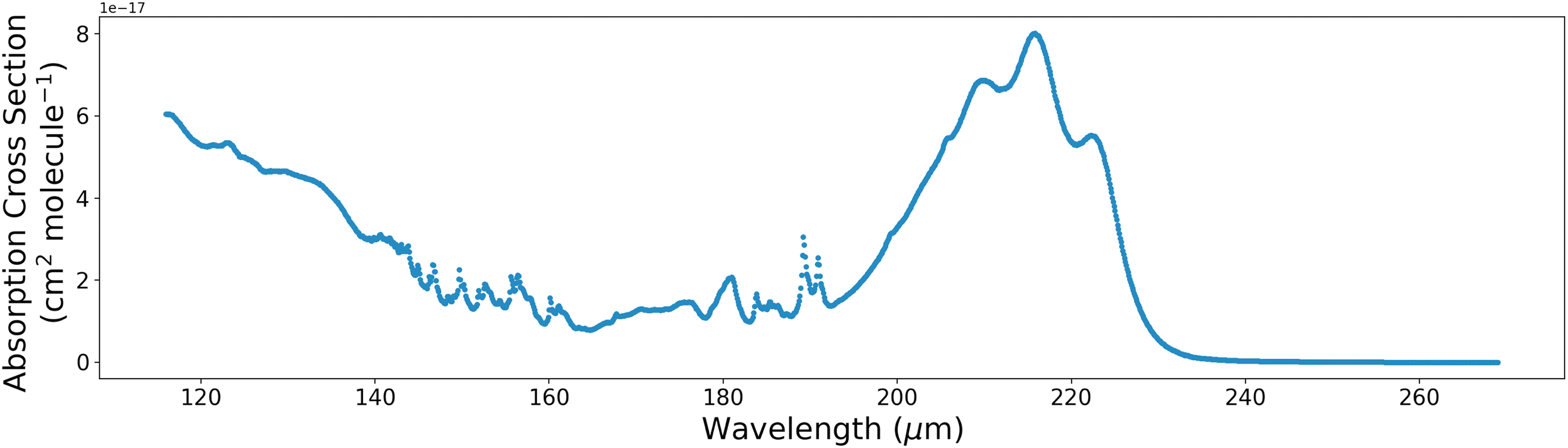
Isoprene UV-Vis absorption cross-section taken from (Dillon et al., 2017). The axes show absorption cross-section (cm2/molecule) versus wavelength (μm). The peak absorption of isoprene UV-Vis is at 218 nm. UV-Vis, ultraviolet-visible. Color images are available online.
3.1.2. IR cross-sections and uncertainty estimates
The isoprene IR absorption cross-sections are shown in Fig. 8. The data are measured by Brauer et al. (2014) and are collected and calibrated by the “HITRAN online Absorption Cross Sections Database” (Gordon et al., 2017).
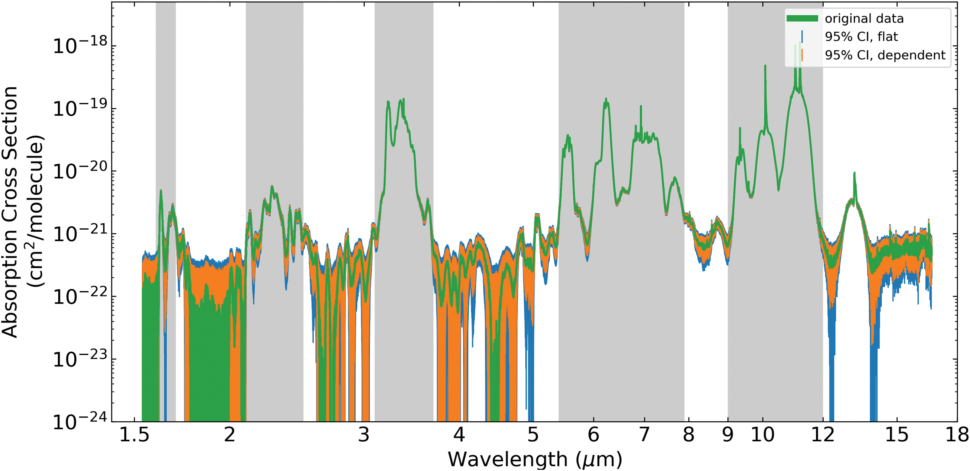
Isoprene high-resolution IR cross-sections at standard pressure and temperature in log-log scale from 1.3 to 18 μm. Shown in green are isoprene cross-sections, as collected by Brauer et al. (2014) and calibrated by HITRAN (Gordon et al., 2017). Shown in blue are the isoprene cross-sections with a uniform uncertainty of 3 × 10⁻²² cm2/molecule. Shown in orange is the estimated wavelength-dependent uncertainty based on methods described in the work of Chu et al. (1999). The uncertainties represent the 95% confidence interval of the data. Marked in gray are the five regions of isoprene spectral features that we consider to evaluate the detectability of isoprene (1.6–1.7, 2.1–2.5, 3.1–3.7, 5.4–7.9 and 9–12 μm). We omit assessment of the spectral features in other regions due to high uncertainties and omit features longer than 12 μm due to high instrumental noise from the JWST MIRI LRS Instrument (Batalha et al., 2017). IR, infrared; JWST, James Webb Space Telescope. Color images are available online.
The isoprene cross-section datasets are measured at standard pressure for 278 K, 298 K, and 323 K with a 1/8 cm−1 resolution. In this study, we opt to only use the 298 K data to assess the detectability of isoprene because it has the least uncertainties. More specifically, measurements at standard pressure and temperature do not require heating/cooling of the experimental setup, and will, therefore, have the least variation between the source and background reference spectra. As a side note, the methodology for the consideration of the noise floor differs between the 298 K data and the 278 K/323 K data. As a result of this difference in treatment, it is not possible to reliably extrapolate the measured cross-sections to temperatures beyond those measured. Including all three measurements with different noise floor treatments may introduce additional uncertainties to our models.
Unlike absorption cross-sections calculated from molecular line lists, the uncertainties of absorption cross-sections calculated from lab-measured transmission spectra cannot be ignored, especially for data points with opacities that approach the instrument noise floor.
We estimated the wavelength-dependent uncertainties (95% confidence interval of the measured data) as described in Eq. 4 in the work of Chu et al. (1999) as follows:
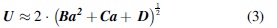
where U is the expanded uncertainty, a is the absorption-cross section, and B, C, and D are coefficients unique for each molecule. The uncertainty U is the 95% confidence interval. We compare the wavelength-dependent uncertainties with a uniform 3 × 10⁻²² cm2/molecule noise floor, as described in the work of Brauer et al. (2014) and approximately validate this method by finding the same averaged value. Therefore, both methods are sufficient to identify which data points we can trust and which may be no different than noise, but in general, the uncertainty of the wavelength-dependent method scales with the cross-section values (uncertainties for the largest peaks are larger than the uniformed uncertainty, and uncertainties for the small peaks near the noise floor are smaller than the uniformed uncertainty).
We note that the specific values of the B, C, and D coefficients for isoprene are not measured by Chu et al. (1999); they are not provided in the original work of Brauer et al. (2014) and are also missing in the NIST spectral database (Linstrom and Mallard, 2001). We, therefore, adopt the values of B = 1.6 × 10⁻⁴, C = 1.1 × 10⁻⁹, D = 2.7 × 10⁻¹⁴ from C4H6 (1-3-butadiene). Although we expect this substitution to introduce some additional uncertainty, it is the most appropriate approximation; C4H6 is structurally similar to isoprene (2-Methyl-1,3-butadiene), though it has one less methyl group.
3.1.3. Isoprene spectral features
Isoprene has 33 fundamental IR-active vibrational modes, associated with several functional groups containing carbon–carbon and carbon–hydrogen bonds. The fundamental vibrational modes of isoprene have previously been assigned from both measured and theoretically calculated spectra (Panchenko and De Maré, 2008; Brauer et al., 2014).
We assess the detectability of isoprene in the context of JWST's observation capabilities (see Sections 3.4 and 4.2). We have divided the isoprene spectral features into five wavelength regions: 1.6–1.7, 2.1–2.5, 3.1–3.7, 5.4–7.9, and 9–12 μm. We omitted spectral features in other regions due to the high measurement error-bars and omitted spectral features above 12 μm due to the high instrumental noise of JWST Mid-Infrared Instrument Low-resolution Spectrometer beyond 12 μm (Batalha et al., 2017).
Isoprene cross-section features in the 1.6–1.7 and 2.1–2.5 μm regions are formed by rovibrational overtones of the 3.1–3.7 μm region bands. Features in these two regions lack reliable experimental measurements (Brauer et al., 2014), and detectability of these two spectral features should be taken with some caution. This article motivates future measurements and theoretical simulations of isoprene spectra in the visible and near-IR, as it would expand the assessment of isoprene detection by using more readily available instruments that cover these spectral regions.
Isoprene spectral features in the 3.1–3.7 μm region primarily comprise the following two features: (1) the narrow bands around 3.2 μm, which are composed of the ν1 and ν2 asymmetric stretching modes; (2) the broader bands (3.3–3.7 μm), which are composed of the ν3 (symmetric stretch), ν4 (asymmetric stretch), and ν24 (deformation) modes (Brauer et al., 2014). These two features arise from the stretching modes of X = C-H (sp2 hybridized) and X-C-H (sp3 hybridized), where X denotes another atom (other than H).
Isoprene spectral features in the 5.4–7.9 μm region comprise the following two features: (1) the narrow features around 6.5 μm, which are composed of the symmetric and asymmetric stretching modes (ν8 and ν9) associated with the C = C double bond; (2) the features in the 6.6–7.9 μm region that are composed of the ν10–13 and ν24 modes associated with deformation and scissoring rovibrational motions (Brauer et al., 2014).
Isoprene spectral features in the 9–12 μm region comprise several bands associated with the wagging modes of the carbon–hydrogen functional groups (ν26, ν27, and ν28), and one associated with the rocking motion of the X = C-H functional group (ν17 mode) (Brauer et al., 2014).
3.1.4. Haze extinction cross-section
We anticipate that abundance of isoprene, a hydrocarbon, in an atmosphere could lead to the presence of a haze layer in the atmosphere similar to the haze layer induced by organic molecules described in the work of Arney et al. (2018). The presence of a haze layer may hinder detection of isoprene spectral features and should be quantified.
Studying the effects of isoprene-induced haze requires wavelength-dependent refractive indices and haze particle size distribution, but neither is available for isoprene as studies regarding reactions of the isoprene-induced radicals (or products of isoprene reactions described in Section 2.3) are limited. Isoprene-induced haze on the Earth does not have measurements in IR thus far, and in any case, the Earth's isoprene-induced haze is an oxygenated product not likely to be the same as the isoprene-induced haze on an anoxic exoplanet. Therefore, we estimate the isoprene-induced haze extinction cross-section by using wavelength-dependent refractive index measurements and haze particle-size distributions of other hydrocarbons in a reducing environment.
We adopt the wavelength-dependent refractive indices of Titan's methane-induced haze (measured by Khare et al., 1984), or tholins, as a proxy for that of isoprene-induced hazes. In our solar system, Titan (Khare et al., 1984), Pluto (Zhang et al., 2017), and Venus have extensive haze layers in their atmosphere. The composition of Pluto's haze is yet to be confirmed. The Venusian haze is not known, but it is likely to contain high concentrations of sulfur-containing molecules derived from SO2 and H2SO4 (Takagi et al., 2019). Therefore, Titan's atmospheric haze is the closest analogue to isoprene haze on habitable exoplanets; both are hydrocarbon-induced haze. To show that our results are not specific to the case of Titan tholins, we compare our results with those using refractive indices of HCN (Khare et al., 1994), C2H2 (Dalzell and Sarofim, 1969), and octane (Anderson, 2000).
We approximated the mean size distribution as a Gaussian distribution with a mean particle size equal adopted from the works of He et al. (2018) and Hörst et al. (2018), who measured the diameters of haze particles for different temperatures and metallicities. For CO2-dominated and N2-dominated atmospheres, we used a mean size of 89 nm and a standard deviation of 25 nm, which is approximated from the 300 K, 1000 × metallicity case from the work of He et al. (2018). For H2-dominated atmospheres, we used a mean size of 53.8 nm and a standard deviation of 16 nm, which is approximated from the 300 K, 10,000 × metallicity case from the work of He et al. (2018). We choose to use a Gaussian distribution approximation rather than using the original measurement to avoid overfitting the data for isoprene.
Finally, we used miepython ** to calculate the isoprene-induced haze's extinction cross-section with the assumed wavelength-dependent refractive indices and haze particle-size distribution. The cross-section is averaged from 1000 radii sampled from the Gaussian distribution. For simplicity, we assumed the haze particle to be spherical and we assumed the mean size and size distribution to be constant as a function of height.
3.2. Photochemistry model
We use the photochemical model from the work of Hu et al. (2012) to calculate the concentration of isoprene in exoplanet atmospheres as a function of surface production flux. The code includes photolysis, reactions with radicals and molecules, dry deposition to the surface, and rainout as sinks of atmospheric gases. The code has been validated by computing the atmospheric composition of current Earth and Mars, matching observations of major trace gases in both atmospheres. The photochemical model by Hu et al. (2012) has been used in a variety of papers (e.g., Sousa-Silva et al., 2020); we provide a brief summary description of our photochemical model here.
The Hu et al. (2012) photochemical model computes the steady-state chemical composition of a planetary atmosphere scenario. We have adapted the model to include isoprene, including photolysis, rainout, and reactions with O⋅, O3, and ⋅OH as sinks on isoprene. Due to the lack of reaction network studies for isoprene-induced radicals in anoxic environments, we assumed that fractions of the photochemical products of isoprene result in haze formation whereas the rest is not tracked; we note that this assumption formally underestimates isoprene concentrations, as haze will shield isoprene from UV photolysis. By contrast, our lack of a detailed reaction network means that we may omit chemical cycles by which the destruction of one molecule of isoprene may lead to additional destruction; this may lead to overestimates of isoprene concentrations. More detailed characterization of the reactions of isoprene and its products are required to resolve this challenge. In Section 4.3, we discuss how different assumed haze-to-isoprene mass fractions (from 1 ppm to 10%) will impact the effect of haze on the transmission spectra. We assume the mass fraction to be constant as a function of height.
The model handles more than 800 chemical reactions (and photochemical reactions), formation, and deposition for aerosols (including elemental sulfur and sulfuric acid); our exoplanet scenarios (Section 3.3) employ a subset of ∼450 of the reactions, excluding primarily nitrogen chemistry and high-temperature reactions (see Hu et al., 2012 for the rationale for these choices). The model also treats dry and wet deposition, thermal escape, and surface emission. The model is flexible to simulate both oxidized and reduced conditions. The model uses delta-Eddington two-stream method to compute the UV and visible radiation in the atmosphere. The optical depth used is calculated with molecular absorption, Rayleigh scattering, and aerosol Mie scattering.
The stellar UV spectral flux data is an input for the photochemistry code. We take the input stellar fluxes from the work of Seager et al. (2013). For the UV flux from a solar-type star, Seager et al. (2013) used the Air Mass Zero (AM0) reference spectrum produced by the American Society for Testing and Materials (
3.3. Simulation scenarios
We now describe our exoplanet benchmark scenarios. Our exoplanet benchmark scenarios are based on those in the works of Hu et al. (2012) and Seager et al. (2013); they are also used in the work of Sousa-Silva et al. (2020). Later, we discuss in detail the 6 simulation scenarios considered here, representing H2-dominated, N2-dominated, and CO2-dominated atmosphere, each exposed to a Sun-like star and an M dwarf star.
3.3.1. Astronomical scenarios
We consider stellar irradiation environments corresponding to the modern Sun and an M5V star (“M dwarf star”) with a visual magnitude of 10.
The semimajor axes of the planets are taken to be 1.6, 1.0, and 1.3 AU if orbiting a Sun-like star, and 0.042, 0.026, and 0.034 AU if orbiting an M dwarf star for H2-dominated, N2-dominated, and CO2-dominated atmosphere, respectively. The semimajor axes are chosen to maintain a surface temperature of 288 K (Hu et al., 2012).
We calculate photochemical models for an Earth analog planet (1 Earth-mass, 1 Earth-radius). We follow the work of Hu et al. (2012) in projecting these photochemical models to the scenario of a massive super-Earth with 10 Earth-mass and 1.75 Earth-radius, by assuming the molecular mixing ratio to be a function of pressure, which is invariant of surface gravity. The preference for the larger planet is beneficial for observation with near-future space telescopes for mass measurement with radial velocity and atmosphere characterization with both transmission (e.g., more likely to retain a reducing, H2-dominated atmosphere) and secondary eclipse spectroscopy (e.g., higher planet/star flux ratio).
3.3.2. Atmospheric scenarios
We consider three different atmosphere scenarios according to their redox state: a reducing H2-dominated atmosphere, an intermediate redox state N2-dominated atmosphere, and a weakly oxidizing CO2-dominated atmosphere. We only consider anoxic atmospheres, because it is already well known from the Earth's atmosphere that isoprene cannot accumulate in an O2-dominated atmosphere. The exact composition and vertical mixing ratio profile for the starting atmosphere scenarios that we use as seeding conditions for calculating vertical mixing ratio profiles with varying surface flux are shown in Supplementary Appendix A1 (and originally come from Sousa-Silva et al., 2020) for details on the H2-dominated and CO2-dominated atmosphere scenarios. The physical concept behind the H2-dominated atmosphere scenario is that the planet outgassed H2 during planet formation and managed to either maintain its H2 atmosphere or has interior reservoirs with planetary processes to replenish it (Table 1).
Atmosphere Composition Adopted from Photochemistry Output of Hu et al. Model for the Six Simulation Scenarios Considered
For spectroscopy calculation and detection assessment, we only consider molecules that have reached a local mixing ratio of at least 100 ppb at any height in the atmosphere. Molecules that fail to meet this mixing ratio criterion are unlikely to contribute sufficient opacity to the simulated transmission and emission spectra and are, therefore, not included. Molecules more than 100 ppm at any height are marked in bold. For detailed mixing ratio profile, see Supplementary Appendix Fig. A1. Addition of isoprene may drastically change the mixing ratio profile for some molecules (see Fig. 9).
C2H6 = ethane; CH4 = methane.
Adapted from Hu et al. (2012).
3.3.3. Atmosphere temperature, pressure, and abundances
Using the six starting simulation scenarios (three atmosphere scenarios for the Sun-like star and three for the M dwarf star) as seeds, we calculate the mixing ratio profile of isoprene with varying surface flux by using the photochemistry code from the work of Hu et al. (2012) for each scenario. The vertical mixing strength (Eddy diffusion profile) of an atmosphere archetype is linearly scaled from the ratio of the Earth atmosphere's mean molecular mass and the atmosphere archetype. We adopt the eddy diffusion coefficients scaling factors of 6.3, 1.0, and 0.68 for the H2-, N2-, and CO2-dominated atmospheres from the work of Hu et al. (2012), which is based on the scale height of the atmosphere archetypes.
The surface pressure of the planet is set to 1 bar, and the surface temperature is set to 300 K. In the troposphere, the temperature decreases with altitude based on a dry adiabatic lapse rate. The tropopause is set to 160 K for the H2-dominated atmospheres, 180 K for the CO2-dominated atmospheres, and 200 K for the N2-dominated atmospheres. The different tropopause temperatures used for each atmosphere reflect the different efficiencies of gases as coolants in the upper atmosphere. H2 is a more effective coolant than N2, so the stratosphere of H2-dominated atmospheres will be colder than N2-dominated atmospheres.
Temperatures above the troposphere are set to be constant, that is, no temperature inversion (see Supplementary Appendix A1 for the temperature-pressure profiles for the three-atmosphere archetypes). This assumption may be violated for hazy atmospheres, where absorption of UV photons by high-altitude haze may drive an inversion, analogous to ozone in the modern Earth's atmosphere. We expect our results to be relatively insensitive to the stratospheric temperature since the ultimate limit on accumulation of isoprene comes from UV photolysis. Nevertheless, we performed a sensitivity test of the resulting transmission spectra by replacing the temperature-pressure profile with that of the Earth's temperature-pressure profile. We find that there is negligible difference in the transmission spectra resulting from the two different temperature-pressure profiles.
We exclude trace gases that do not exceed 100 ppb at any altitude from our spectral model, because their absorption does not contribute enough variation to the atmosphere spectra and they are unlikely to be detectable without significant instrumentation advancements that are capable of reaching a < 1 ppm noise floor.
3.4. Atmosphere spectra simulation
To assess the detection of trace gases and biosignature gases in exoplanet atmosphere scenarios, we constructed the “Simulated Exoplanet Atmosphere Spectra” (SEAS;
The molecular cross-sections used by SEAS are interpolated from a pre-generated grid of cross-sections for a grid of pressure (105 to 10−2 Pa in multiples of 10) and temperature (150–400 K in steps of 25 K). For molecules that have line lists from the work of Gordon et al. (2017), the cross-sections are calculated by using the HAPI package (Kochanov et al., 2016). For molecules that have line lists in ExoMol (Tennyson et al., 2016; Gordon et al., 2017), cross-sections are calculated by using the ExoCross package (Yurchenko et al., 2018).
We validated SEAS by generating Earth spectra and comparing transmission spectra results with data from the Atmospheric Chemistry Experiment data set (Bernath et al., 2005) and comparing emission spectra with results from MODerate resolution atmospheric TRANsmission spectrum simulation code (Berk et al., 1998).
3.4.1. Transmission spectra
The SEAS transmission spectrum code calculates the radiative transfer of stellar radiation passing through each layer of the transiting planet atmosphere. Next, we detailed the exact step to calculate the effective height of the atmosphere and the transit depth for each wavelength.
We defined each layer of the atmosphere with a height of 1 scale height starting from the surface to the top of the atmosphere and assumed local thermodynamic equilibrium within each layer of the atmosphere.
Since the atmosphere is taken to be homogenous within each layer, we approximate the three-dimensional spherical shell as a two-dimensional ring.
Since each layer is curved and stellar radiation is radial, the stellar radiation along the limb path of each layer will penetrate sections of the current layer and sections of layers above the current layer. Therefore, the optical depth of each layer is the sum of the optical depth through each section as follows:

where A(λ)i is the total wavelength-dependent absorption for the i th layer, j denotes each molecule, n is the number density, σ(λ) is the wavelength-dependent absorption cross-section, P is the pressure, T is the temperature, l is the path length, z denotes the total number of layers above the i th layer that the stellar radiation passes through, and m denotes the total number of molecules.
The transmission by each layer is calculated by using Beer-Lambert's Law: T = e −A , and absorbance is 1-T.
The effective height of the atmosphere is calculated by summing the effective height of each layer, which is calculated by multiplying the absorbance by the scale height of each layer.
The transit depth of the atmosphere is calculated by summing the flux attenuated by each layer of the atmosphere, which is calculated by multiplying the absorbance by the cross-sectional area of each layer.
We note that the cross-sections of haze particles have units of (cm2/particle) and, therefore, the particle density is calculated from the gas number density and has a unit of (particle/cm3). The particle density of isoprene-induced haze at a given layer is calculated by dividing the particle vapor density with the average particle mass. The particle vapor density is the product of the air density, the mixing ratio of isoprene, and an assumed haze-to-isoprene mass fraction (see Section 3.2).
To consider the detection of isoprene via transmission spectra, we first assessed model scenarios in which the atmospheres have no clouds or haze. This result represents an upper bound on the detectability of the isoprene features in transmission (Section 4.2). Next, we study how detection will be hindered if haze is included (Section 4.3).
3.4.2. Secondary eclipse thermal emission spectroscopy
The SEAS thermal emission code is similar to those described in the works of Seager (2010) and Sousa-Silva et al. (2020) and uses the same temperature-pressure profiles, mixing ratio profiles, and molecular-cross sections as in the transmission code.
The emission code integrates the blackbody radiation for each wavelength from the surface and up through each layer of the atmosphere, as the radiation is absorbed and reemitted by gases in each layer. The surface is set to be a pure black body, and the top layer is set to be transparent. We do not consider scattering in the current emission code. The final spectrum is calculated by integrating the emerging flux by the cross-sectional area of the planet. To add the presence of clouds, we consider 50% cloud coverage by averaging between a cloudy and cloud-free spectrum.
3.5. Simulated exoplanet observation
We simulate observations of the six simulation scenarios as described in Section 3.3.2 with varying amounts of isoprene as computed by our photochemistry model in Section 3.2. We used the astronomical parameters defined in Section 3.3.1 and a 10 M Earth, 1.75 R Earth-planet transiting a star with a K-band apparent magnitude of 10 (JWST observes in near-mid IR). The star can be either (1) a Sun-like star or (2) a 3000 K, 0.26-Rsun M dwarf star.
Since isoprene has many broad spectral features spanning a wide range of wavelength as discussed in Section 3.1.2, we opt to assess the detection of isoprene by using JWST's Near InfraRed Spectrograph (G140M, G235M, G395M) and MIRI (LRS) observation modes.
For transmission spectroscopy, we combined the simulated spectra from SEAS and observational noise simulated by using Pandexo (Batalha et al., 2017), the community JWST exposure time calculator, and noise simulator. To account for potential unknowns, we added a 10 ppm noise floor as suggested by Batalha et al. (2017).
For secondary eclipse thermal emission spectroscopy, we approximate our telescope specifications based on JWST and the use of the NIRSpec and MIRI instruments (Bagnasco et al., 2007; Wright et al., 2010), or a 6.5 m space telescope with a quantum efficiency of 25%. Since stellar flux is the source of the noise, we do not model instrumental noise and instead used a 50% photon noise multiplier. Finally, we compute the signal-to-noise ratio for each bin by using the equation given next:
where Fin is the flux density within the absorption feature, Fout is the flux density of the surrounding continuum of the feature, and σFout and σFin comprise the respective uncertainty.
Although we have estimated instrumental noise, our estimates on stellar noise remain rudimentary. We raise the caveat that additional sources of astrophysical noise may make detecting molecular features challenging. Other astrophysical phenomenon, such as non-homogeneity of stellar disks, could introduce false spectral features from 0.3 to 5.5 μm with intensities around 70 ppm for M5V stars (Rackham et al., 2018), potentially hindering the detection of biosignature gases.
3.6. Biosignature gas detectability assessment
Determining the detectability of a biosignature gas in our atmosphere scenarios is expanded based on the methods defined in the works of Seager et al. (2013), Tessenyi et al. (2013), and Sousa-Silva et al. (2020), where we assess whether the spectral features of the target biosignature gas can be identified within a reasonable number of transit (secondary eclipse) observations.
First, we assess whether or not the atmosphere (and the biosignature gas) can be detected by applying a null-hypothesis test. More specifically, we assess whether or not the simulated wavelength-dependent transit depth data can be explained with a straight line (transmission) or with a blackbody radiation curve (emission). If so, then the simulated observation cannot pass the null-hypothesis test and we deem the atmosphere scenario to be not-detectable.
Next, if the simulated observation for the atmosphere scenario passed the null hypothesis, we then compare the goodness-of-fit of a model atmosphere that contains the biosignature gas and a model atmosphere without the biosignature gas. The goodness-of-fit is computed by using the reduced chi-square statistic using the following equation:

where χν 2 is the reduced chi square, ν is the degree of freedom (or the number of wavelength bins), χ 2 is the chi squared, Oi is the simulated observational data, Ci is the simulated model, σi is the variance (or error as calculated from Pandexo noise simulator for a specific instrument), and finally i denotes each wavelength bin. We note that binning the spectra reduces the variance at the expense of reducing the degree of freedom.
The simulated observation data has moderate spectral resolution (R > 1000 for NIRSpec and R = 160 for MIRI) but also has large error bars for each data point. Since we are interested in detecting the broad spectral features of isoprene and not the narrow, detailed individual features, we can trade resolution for increased SNR to improve our model's goodness-of-fit. R = 10–20 is where isoprene becomes indistinguishable with methane for features at shorter wavelengths (<4 μm), and this concept will be further explored in Section 4.3.
Finally, we repeat calculation of the detection metric cited earlier by binning down our simulated spectra to spectral resolutions of R = 10, 20, 50, and 100 to find the most optimal choice and iterate from 1 to 100 transits until detection is reached. If no detection is found with any spectral resolution and 100 transits (theoretical upper limit for a planet in the habitable zone of an M dwarf star given JWST's expected cryogenic lifetime of 5 years), we deem the spectral features not detectable.
4. Results
Despite its promising potential, isoprene does not satisfy all criteria to be a good biosignature gas. Namely, isoprene is unable to accumulate in the upper atmosphere at even 10 times the Earth's production level, and in fact isoprene must enter a “run-away phase” to accumulate to detectable abundances. In addition, isoprene can be spectrally indistinguishable from methane at short wavelengths (<4 μm) with JWST's spectral resolution. Regardless of this, isoprene should still be added into the roster of biosignature gas to be considered in future studies because isoprene has no abiotic false-positives and it has the potential to be produced in large quantities as it is by life on the Earth.
We demonstrate that with the Earth's production rate, isoprene molecules are predominantly concentrated near the surface (<10 km) (Section 4.1.1), making detection impossible with near-future technologies (Section 4.2.1). An additional key point is that with a production rate 100–1000 times higher than the Earth's isoprene production rate—which we assert is challenging but within reasonable estimates (Section 4.1.2)—isoprene can enter a run-away phase, enabling isoprene molecules to populate the upper atmosphere at a significant concentration (>100 ppm) (Section 4.1.3) and become detectable (Section 4.2.2).
Unfortunately (within the context of observing the atmosphere of a super-Earth with JWST), despite its detectability in a run-away phase, we show that isoprene's spectral features can be confused with those of methane and other hydrocarbons More specifically, isoprene spectral features at 3.1–3.7 μm overlap with that of methane. Moreover, isoprene's spectral features at 9–12 μm lie in a wavelength region populated by hundreds of other hydrocarbon gases (Section 5.2). On the Earth, any isoprene is immediately converted into haze, so we also discuss the impact of haze on hindering the detection of isoprene (Section 4.3).
Far-future telescopes that can achieve detection at higher spectral resolution than JWST may make detection of isoprene possible. Therefore, given the abundant chemical reactions involving isoprene in known biochemistry and the fact that it does not have any abiotic false positives (Section 4.3), it would be hasty to discard isoprene as a potential biosignature gas.
4.1. Isoprene accumulation
We calculated the column-averaged mixing ratio profile of isoprene and other gases as a function of surface isoprene flux, using the photochemistry code described in Section 3.3. We list the column-averaged mixing ratio for isoprene given the surface production rate for each simulation scenario in Table 2.
Isoprene Column-Averaged Mixing Ratios (in Units of ppm) Corresponding to Various Isoprene Surface Fluxes (i.e., Production Rates) for Our Six Atmosphere Archetypes
For reference, biological production of isoprene on Earth is ∼500 Tg/year, or 2.7 × 10¹⁰ molecules/(cm2·s) and biological production of CH4 on Earth is also about 500 Tg/year, or 1.2 × 10¹¹ molecules/(cm2·s). Our photochemistry model simulated equilibrium atmospheric abundances for a range of surface fluxes from 103 to 1015 molecules/(cm2·s). Fluxes <1010 and <1013 molecules/(cm2·s) are omitted for M dwarf star and Sun-like stars, respectively, because the resulting column-averaged mixing ratios are negligible (<1 ppb). Fluxes >1013 molecules/(cm2·s) are omitted for M dwarf stars, because isoprene reaches a run-away phase and to exceed 1% of the atmosphere by volume, a likely unrealistic value. Omitted entries are denoted by the “/” symbol. The column-averaged mixing ratio quickly transitions from <1 to >100 ppm around 1012–1013 molecules/(cm2·s) surface flux values.
To assess isoprene's ability to accumulate in an atmosphere, we first examine the distribution of isoprene in an exoplanet atmosphere given a production rate similar to that on the Earth, ∼3 × 10¹⁰ molecules/(cm2·s) (Section 4.1.1). Next, to go beyond the Earth's conditions, we calculate isoprene mixing ratio profile for a range of isoprene surface production rates. We vary the production rate from 103 molecules/(cm2·s) to 1015 molecules/(cm2·s) in steps of 10. We choose a maximum of 1015 molecules/(cm2·s) to represent the highest isoprene production rate found in a niche environment on Earth (Section 4.1.2).
4.1.1. Isoprene remains a trace gas at Earth's production rate
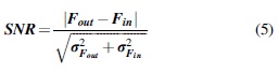
At the Earth's isoprene production rate of 3 × 10¹⁰ molecules/(cm2·s), isoprene remains a trace gas in all of the three exoplanet atmosphere scenarios, at <1 ppb (column-averaged mixing ratio) (Table 2). At surface fluxes lower than 1 × 10¹¹ molecules/(cm2·s), isoprene is concentrated near the surface where it is created. Any isoprene that diffuses to the upper atmosphere is readily destroyed. To illustrate this finding, the column-averaged mixing ratio of isoprene at four different altitudes for a CO2-dominated atmosphere of an exoplanet transiting an M dwarf star is shown in Fig. 9.
Column-averaged mixing ratios of isoprene and other major atmospheric gases in a CO2-dominant atmosphere orbiting an M dwarf star as a function of isoprene surface flux. Dominant atmosphere species and isoprene-reacting radicals are plotted in various colored dash lines. The isoprene column-averaged mixing ratios (in units of ppm) for different isoprene surface fluxes [i.e., biological production rate; in units of molecules/(cm2·s)] are shown by a solid black curve. The abundance of isoprene at 0–10 km from the surface overlap with the solid black curve and is additionally indicated by the light gray stars. The abundances of isoprene at 10–20, 20–30, and >30 km from the surface are shown in different shades of gray and are additionally shown by different types of triangles. For low surface fluxes, isoprene remains a trace gas throughout the atmosphere (<ppm levels) with abundances increasing linearly with surface fluxes. For surface fluxes above 3 × 10¹⁰ molecules/(cm2·s), isoprene abundance rapidly increases. For isoprene surface fluxes above 3 × 10¹¹ molecules/(cm2·s), isoprene abundance at the upper atmosphere (where most transmission spectral features originate) reaches the same level as surface abundance. Color images are available online.
Isoprene may remain a trace gas even at higher production rates than on the Earth, because large isoprene sinks may exist on planets different from the Earth. The sinks could realistically include life that has evolved to consume the abundant isoprene; photochemical destruction pathways as yet-unknown in anoxic atmospheres; and/or higher deposition rates than those that exist on the Earth.
As a trace gas, isoprene is not detectable via transmission spectroscopy even with far-future space telescopes. In Section 4.2.1, we explore the potential to detect isoprene as a trace gas via thermal emission spectroscopy by using JWST.
4.1.2. Maximum isoprene production estimate
For isoprene to accumulate to higher levels than a trace gas, it must be produced by life at rates hundreds, if not thousand times, the global production rate on the Earth (Fig. 9). In this section we establish that high isoprene production niche environments exist on the Earth, up to one million times the Earth's globally averaged isoprene production rate (Section 2.2).
One such niche is a modern tropical environment, where isoprene production is optimal for trees, the main producer of isoprene on the Earth due to their widespread abundance. In the Amazon rainforest, African rainforest, and Southeast Asia, the isoprene production rate averages >1 mg/(m2·s) with core areas averaging >10 mg/(m2·s) (McFiggans et al., 2019). In comparison, the global averaged isoprene production rate on the Earth is ∼3 × 10⁻⁵ mg/(m2·s) [converted from 500 Tg/year, or ∼3 × 10¹⁰ molecules/(cm2·s)]. For 12% of the Earth's habitable history [e.g., during Phanerozoic eon (the past 541 million years)], the Earth had a pole-to-pole tropical climate (e.g., during Carnian Pluvial Event; Royer et al., 2004; Dal Corso et al., 2012). Therefore, in a hypothetical scenario where the Earth's total land mass (∼30% of total surface area) is filled completely with isoprene producers and attains the 1 mg/m2 production rate, it is possible for the global average to reach 0.3 mg/(m2·s), or 3 × 10¹⁴ molecules/(cm2·s). However, although trees are the main producer of isoprene on the Earth, we cannot ignore the fact that trees are also the main producer of oxygen and the presumed condition for isoprene to accumulate is an anoxic atmosphere.
For a purely anoxic environment, we assume an Archean biosphere that comprises anaerobic, isoprene-producing prokaryotes such as those found in lab studies (Fall et al., 1998) (see Section 2.2 for details), which is capable of naturally producing isoprene in high quantities with average production rates of 50 nmol/(g·hour). By using an average bacteria density of 1 g/cm3 (Loferer-Krößbacher et al., 1998) and assuming a global biomass layer of 1 cm thick covering all of the Earth's total land mass (∼30% total surface area), it is possible for the global average to reach 2.5 × 10¹³ molecules/(cm2·s).
With these assumptions, we show that the high isoprene production rates required for isoprene to accumulate in the upper atmosphere can be supported by species on Earth and the theoretical upper limit to isoprene production rate is 104 that of the Earth's current production rate. Therefore, it is plausible to explore the detection of isoprene under these conditions.
4.1.3. Isoprene run-away
Very high surface fluxes of isoprene will send isoprene accumulation into a run-away state (Fig. 9). In a run-away phase, isoprene rapidly accumulates in the upper atmosphere to high levels, up to hundreds of ppm. The run-away is a result of “photochemical self-shielding” whereby the isoprene production flux saturates its UV-driven sinks, resulting in a dramatic increase in lifetime and hence accumulation. This run-away phenomena has been discussed for abiotic CO (Kasting et al., 1983, 1984, 2014; Zahnle, 1986; Kasting, 2014), has been alluded to for CH4 (Segura et al., 2005), and has been observed by us for other biosignature gases (Huang et al., unpublished data; Sousa-Silva et al., 2020). We plan a detailed study in the work of Ranjan et al. (unpublished data). In this subsection, we consider the case where isoprene has entered a run-away phase, a scenario in which the abundance of isoprene in the upper atmosphere reaches a similar level to the abundance of isoprene in the lower atmosphere.
The run-away phase is important, because it shows that cases exist in which isoprene can populate the upper exoplanet atmosphere such that it can be detected via transmission spectroscopy in simulations of the JWST. Recall that transmission spectra are only sensitive to the upper atmosphere. The lower atmosphere has extremely long path lengths for light to travel through it, making the atmosphere optically thick, which, in turn, results in featureless spectra.
The most favorable atmosphere scenario for isoprene accumulation is a CO2-dominated atmosphere because CO2 shields isoprene more strongly from UV irradiation than N2-dominated atmosphere or H2-dominated atmosphere do.
The run-away effect is highly dependent on the quantity of UV flux from the host star. UV fluxes from Sun-like stars are significantly (more than 1000 times) higher than UV fluxes from M dwarf stars. Isoprene is unlikely to enter the run-away phase for planets orbiting Sun-like stars. There, the production rate required is around 3 × 10¹⁴ molecules/(cm2·s) for a CO2-dominated atmosphere, approaching the maximum isoprene production rate even in niche environments on the Earth. In contrast, for planets orbiting M dwarf stars, isoprene's transition to the run-away phase occurs around 3 × 10¹¹ molecules/(cm2·s) for a CO2-dominated atmosphere and 1 × 10¹² molecules/(cm2·s) for an H2-dominated or N2-dominated atmosphere. The surface flux required to enter the run-away phase is within 1–2 orders of magnitude of the Earth's globally averaged surface isoprene flux of 2.7 × 10¹⁰ molecules/(cm2·s). With isoprene surface fluxes above 3 × 10¹¹ molecules/(cm2·s), but below 3 × 10¹² molecules/(cm·s), the corresponding atmosphere volume mixing ratio is 100 ppm or greater, and isoprene can accumulate in the upper atmosphere. At isoprene surface fluxes above 3 × 10¹² molecules/(cm2·s), the corresponding atmosphere column-averaged volume mixing ratio is 1000 ppm (0.1%) or greater. There are sufficient isoprene molecules in the atmosphere to balance photochemical destruction, thus allowing isoprene molecules to diffuse to the upper atmosphere; the resulting mixing ratio profile is well mixed such that isoprene has a constant mixing ratio up to 50 km above the surface.
Therefore, if life produces enough isoprene to enter a run-away phase, isoprene can accumulate to become a major atmospheric gas. In this case, life will have re-engineered the atmosphere, reminiscent of cyanobacteria's oxygenation of the Earth's atmosphere. We note that the run-away hypothesis ignores potential unknown chemical or surface sinks in anoxic atmospheres that would limit the accumulation of isoprene in the atmosphere. Therefore, realistic situations might require further investigation (see e.g., Ranjan et al., unpublished data).
4.2. Isoprene detectability in exoplanet atmospheres
Isoprene detectability can be separated into two categories. The first category is where isoprene does not enter a run-away phase and remains a trace gas (i.e., does not accumulate above a column-averaged mixing ratio of 1 ppm). The second category is where isoprene is a major atmospheric gas, resulting from its production by life at high enough levels that isoprene enters a run-away phase (i.e., isoprene accumulates above a column-averaged mixing ratio of 100 ppm). The transition from a column-averaged mixing ratio of 1–100 ppm occurs rapidly as a function of surface flux (Fig. 9), so we omit discussion of this transition phase.
4.2.1. Detecting isoprene as a trace gas is challenging
As a trace gas, isoprene molecules are concentrated near the surface. We did not find any transmission spectra scenario in which isoprene can accumulate above the troposphere for a surface flux below 1 × 10¹² molecules/(cm2·s). Our spectra simulations confirmed that the isoprene spectral features are <10 ppm in transit depth, smaller than JWST's assumed noise floor. Therefore, it is not possible to detect isoprene as a trace gas via transmission spectroscopy.
We additionally explore whether isoprene can be detected via secondary eclipse thermal emission spectroscopy (emission spectroscopy) for planets transiting an M dwarf star. In emission spectroscopy, spectral features scale with the temperature gradient and, in general, detection might be more promising than for transmission spectroscopy.
For the terrestrial exoplanet atmosphere scenarios we considered in this study, the largest change in temperature occurs in the lower atmosphere layers, from the planet surface to “tropopause.” Therefore, in scenarios where isoprene is a trace gas and concentrated near the surface, it is worth investigating detection via emission spectroscopy.
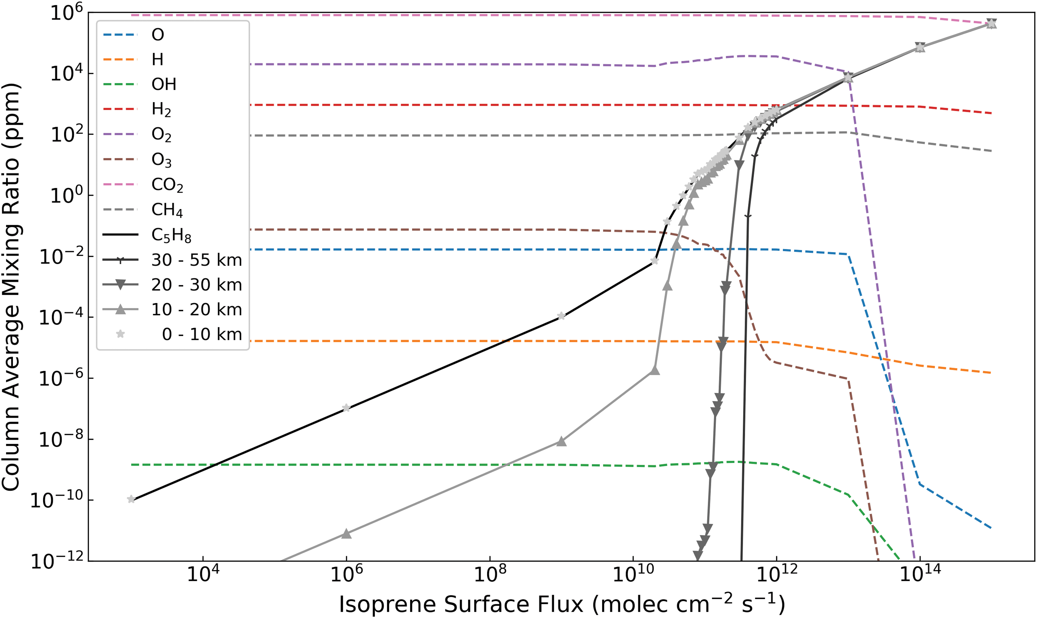
Since isoprene accumulates best in CO2-dominated atmospheres, we modeled this case. We found that in a CO2-dominated atmosphere, secondary eclipse detection for a planet transiting an M dwarf star is possible given a surface flux of 1 × 10¹¹ molecules/(cm2·s), which is three times that of the Earth's isoprene surface flux (Fig. 10). Detection of isoprene in H2- and N2-dominated atmospheres is possible given a surface flux of 1 × 10¹² molecules/(cm2·s). For a planet with a habitable surface temperature of ∼300 K, the peak thermal emission is between 10 and 15 μm. There is only one very broad spectral feature of isoprene that lies in this spectral region, between 9 and 12 μm.
Simulated secondary eclipse thermal emission spectra for an H2-dominated (left) and N2-dominated (right) atmosphere of an exoplanet transiting an M dwarf star with an isoprene surface flux of 1 × 10¹² molecules/(cm2·s). The simulated atmosphere uses input and parameters as listed in Section 3. We show the planet-to-star flux ratio versus wavelength in μm (top) and the statistical significance of a modeled atmosphere versus wavenumber in cm−1 (bottom). The horizontal axes are applied to both the top and bottom panel. In the top panel, we show the simulated atmospheres with and without isoprene as represented by the green and orange curves, respectively. The best fit blackbody curves are shown in blue. Simulated observations of atmospheres with isoprene are represented by the black error bars. In the bottom panel, we show the statistical significance of a simulated atmosphere with isoprene as compared with the black body fit, in units of σ-interval. The green line represents the 5-σ statistical significance threshold. Color images are available online.
Unfortunately, given a spectral resolution of R, approximately 10–20, although we could detect isoprene, it would be hard to distinguish isoprene from other molecules that could be absorbing in this spectral region. Future 30-meter diameter aperture ground-based telescopes with dedicated instruments that focus on the N-band and using a spectral resolution of R > 100 will be able to identify the individual, narrow spectral features that made up the broad 9–12 μm spectral features if given generous observation time (100+ transits).
4.2.2. Detection of isoprene as a major atmospheric gas
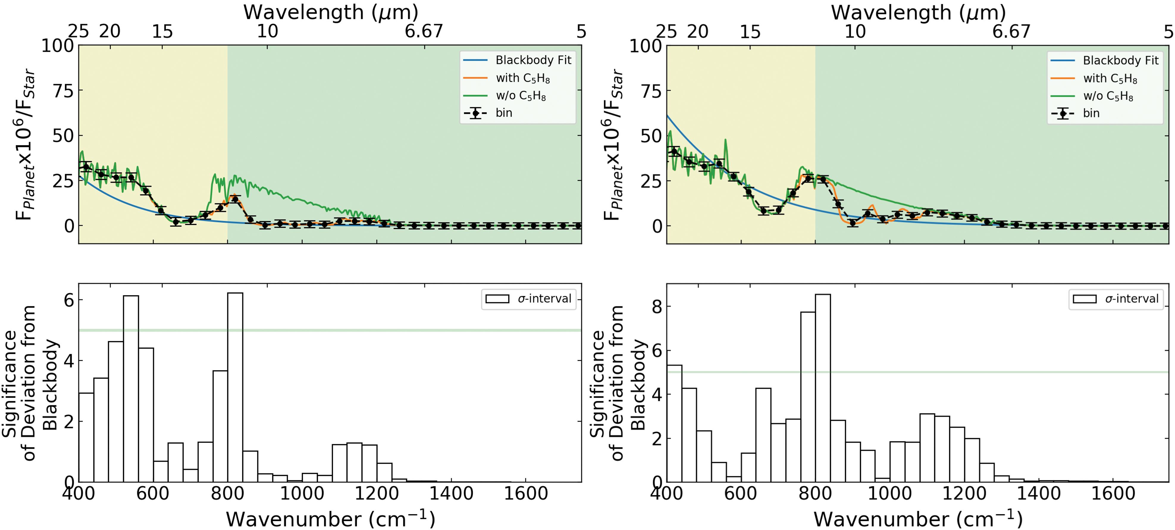
We assess the detection of isoprene via transmission spectra for isoprene in the run-away phase via transmission spectra. For exoplanets with anoxic atmospheres orbiting M dwarf stars, the high isoprene accumulation scenario occurs given an isoprene production rate of at least 1 × 10¹² molecules/(cm2·s) for any atmosphere scenario we studied. We found that at this high production rate, isoprene can accumulate to a column average mixing ratio of 100–1000 ppm and the isoprene spectral features would be prominent compared with those of other molecules, potentially allowing isoprene to be identified (Fig. 11).

Upper panel: Simulated spectra of exoplanets with H2-dominated atmospheres transiting an M dwarf star for a range of isoprene surface fluxes from 0 to 1 × 10¹³ molecules/(cm2 s). The y-axis shows transit depth (ppm), and the x-axis shows wavelength (μm). The spectra are simulated from 0.3 to 23 μm, covering the wavelength span of most of JWST's observation modes. The yellow, green, and blue region shows the spectral coverage of NIRSpec and the red region shows that of MIRI LRS. At low surface mixing ratios, the isoprene spectral features are not prominent as isoprene is mostly concentrated near the surface and rapidly decays as a function of altitude. Isoprene features are not noticeable until the surface flux is above 1 × 10¹¹ molecules/(cm2·s). Above 1 × 10¹² molecules/(cm2·s), increasing the surface flux of isoprene rapidly increases the amount of isoprene in the atmosphere and significantly increases the strength of isoprene's transmission spectral features. Lower panel: Comparison of isoprene cross-sections (Brauer et al., 2014) with cross-sections of dominant molecules (except H2, its absorption is mainly in the form of collision-induced absorption) in the atmosphere such as H2O, CO, CH4, and CO2 (Gordon et al., 2017). Color images are available online.
For terrestrial exoplanets transiting the 10th magnitude M5V dwarf star, only the H2-dominated atmospheres (with surface pressure set to 1 bar and surface temperature set to 300 K) are detectable with JWST in transmission spectroscopy in near- to mid-IR, as they have a large scale height due to the low mean molecular weight. In this scenario, isoprene can be detected if it is produced at fluxes above 3 × 10¹² molecules/(cm2·s), or 100 times that of the Earth's isoprene production rate. Isoprene has many spectral features; we find that detection can be achieved with 20 transits by using any of the four modes of JWST (NIRSpec G140M, G235M, G 395M, and MIRI LRS) we assessed (Fig. 12).

Upper panel: Simulated H2-dominated atmosphere observation using JWST for a 10 M Earth, 1.75 R Earth super-Earth transiting an M dwarf star given 20 transit observations per instrument (80 transits in total). The y-axis shows transit depth (ppm), and x-axis shows wavelength (μm). The simulated observation spans the wavelength range of the NIRSpec and MIRI instruments. We compare a model with no isoprene surface flux (blue line, green error-bar) and a model with 5 × 10¹² molecules/(cm2·s) (orange line, red error-bar). The error bars are 95% confidence intervals for each model uniformly binned to a spectral resolution of R = 10. For this comparison, we take the isoprene cross-section as is and did not account for lab measurement error estimates. The error bar is attributed from observational noise only to more accurately reflect observation simulation. Lower panel: Difference between the two simulated spectra showing the spectral features of isoprene peaks. We show that within each instrument, there are more than more than 20 ppm transit depth differences between the two models; therefore, it is possible to achieve statistical significance and detect isoprene. Color images are available online.
For N2-dominated and CO2-dominated atmospheres, we did not find a scenario in which the atmosphere is detectable via transmission spectroscopy with JWST without investing 100 transits per observation mode. Although it is theoretically possible to accumulate 100 transits for a planet orbiting a late M dwarf star over 5 years (the cryogenic lifetime of JWST), it is unrealistic given the competitive nature of the telescope observation time. We, therefore, conclude that detection of isoprene in a non-H2-rich atmosphere should only be considered plausible for exoplanet dedicated future observatories with far better collecting power.
For exoplanets transiting a Sun-like star, we found that no atmosphere scenarios are detectable via transmission spectroscopy because the ratio of planet to star radius, or (Rplanet/Rstar)2, was too small, resulting in too small a transit depth even for H2-dominated atmospheres.
Assessing the detectability of isoprene as a major atmospheric gas via secondary eclipse thermal emission spectroscopy is at present problematic due to our assumption of an isothermal atmosphere above the 0.01 bar (103 Pa) level (an assumption in our photochemistry model; Hu et al., 2012). Secondary eclipse thermal emission spectra can, in principle, arise in the lower atmosphere, which in our model does have a temperature gradient. However, when isoprene is a major atmosphere gas, above column-averaged mixing ratio of 100 ppm, there are enough isoprene molecules to saturate the atmosphere and render it opaque from the surface to near or above the 0.01 bar level. Since the atmosphere is isothermal above 0.01 bar, the result is a featureless spectrum: a blackbody curve of much lower temperature than the surface temperature (Supplementary Appendix Fig. A2). Correction for this would require adapting the photochemistry model to use a self-consistent temperature-pressure profile, which is beyond the scope of this work.
4.2.3. Isoprene identification is hindered by methane
Detecting isoprene on an exoplanet atmosphere is challenging, requiring either very high isoprene production rate and/or long observation times. Another layer of challenge is that isoprene identification can be hindered by methane, unlike other biosignature gases we proposed: PH3, which have distinguishable features around 4.5 μm (Sousa-Silva et al., 2020), and NH3, which have distinguishable features around 1.5, 2 μm (Huang, et al., unpublished data). Therefore, we report on isoprene spectral distinguishability because, as observing capabilities improve in the future, the ultimate limiting factor for isoprene detection will remain the spectral strength, location, and distinguishability of its features, and these are immutable.
When compared with the expected major gases in habitable terrestrial planet atmospheres, isoprene broad band (R approximately 10–20) spectral features are distinguishable from molecules such as H2O, CO2, CO, NH3, and H2S (see Supplementary Appendix Fig. A3). However, distinguishing isoprene from CH4 will be challenging and requires further discussion. The column-averaged mixing ratio of methane in the six simulation scenarios is in the range between 1 and 100 ppm (see Supplementary Appendix Fig. A1 for detailed mixing ratio profile). For H2-dominated atmospheres, CH4 should be readily present (Seager et al., 2013). In CO2-dominated atmospheres where CH4 may not exist, isoprene contamination by CH4 will not be an issue though other hydrocarbons might still confuse isoprene identification (see Section 5.2 for further discussion).
In an idealistic world with no observational constraints, the spectral features of all molecules are unique. Given the limitation of numbers of photons, however, instruments always have a finite spectral resolution. For detection of habitable exoplanet atmospheres, we must further trade spectral resolution in favor of increasing the (SNR) by binning the data after the data are obtained. We find that the data need to be binned to a relatively low spectra resolution of R = 10–20 to reach statistical significance (as demonstrated in Fig. 12).
At resolution lower than R = 20, distinguishing between isoprene spectral features and methane spectral features at shorter than 4 μm is not possible. Both methane and isoprene share the C-H stretch feature and its overtones; thus, if methane is present in significant quantities, the isoprene 1.6–1.7, 2.1–2.5, and 3.1–3.7 μm features will be masked by methane. In contrast, the 5.4–7.9 μm features and the 9–12 μm features do not overlap with methane spectral features (Fig. 13). Therefore, to confidently detect isoprene in H2-dominated atmospheres, the identification of both the 5.4–7.5 μm features and the 9–12 μm features is required, therefore requiring the use of both NIRSpec and MIRI, potentially more than doubling the number of transit observations required (since there are fewer photons at longer wavelengths).
Comparison of isoprene (orange) and methane (blue) cross-sections binned to R = 20. The axis shows cross-section (cm−2·molecule−1) versus wavelength (μm). Cross-sections for isoprene are measured by Brauer et al. (2014). Cross-section for methane is calculated by using HITRAN line lists with standard pressure and temperature (Gordon et al., 2017). The small panel shows a zoomed-in version of the isoprene-methane-shared spectral feature at 3.1–3.7 μm. We show that distinguishing between isoprene and methane spectral features at 3.1–3.7 μm is still possible at a spectral resolution of R = 20. Distinction between isoprene and methane at spectral resolution lower than this limit is not possible, and, therefore, detection of isoprene's 3.1–3.7 μm feature requires sufficient spectral resolution. We also show that isoprene's 5.4–7.5 μm features and the 9–12 μm features do not overlap with methane's spectral features, so detection of these two features can be done with a lower spectral resolution. Color images are available online.
4.3. Impact of haze on isoprene detection
We turn to an assessment of the detectability of isoprene in anoxic atmospheres with the presence of isoprene-induced haze. We find that haze will hinder but not completely mask the detection of isoprene unless the ratio between the total mass of isoprene-induced haze and the total mass of isoprene (haze-to-isoprene mass ratio) is above 10%. We consider a detection to be hindered if certain spectral features (in a confined wavelength range) are not detectable. We consider detection to be masked if no spectral features are detectable at any wavelength range. We simulate a wide range of scenarios to study how haze abundance, composition, size, †† and size distribution can hinder isoprene detection.
Our models show that the most important factor that affects the detection of isoprene spectral features is the abundance of haze, followed by the size of the haze particles. The abundance of haze governs the overall opacity of the atmosphere, whereas the particle size plays a key role in determining the wavelength dependence of the opacity. Our simulations also suggest that the composition and the mean diameter of the haze particles matter less than the abundance and size distribution.
We quantify how different haze-to-isoprene mass ratios affect a simulated transmission spectrum (Fig. 14). We used our CO2-dominated atmosphere archetype with an isoprene surface flux of 1 × 10¹³ molecules/(cm2·s) and other parameters described in Section 3. A sub-micron ‡‡ size particle's extinction cross-section at wavelengths longer than 3 μm decreases as the wavelength increases. The 1.6–1.7 and 2.1–2.5 μm features are sensitive to haze and can be diminished in strength for a haze-to-isoprene mass ratio of 0.0001. The 3.1–3.7 μm isoprene spectral feature is not affected for a haze-to-isoprene mass ratio of 0.0001 or lower but is masked for a ratio >0.001. The 5.4–7.5 μm spectral feature is not affected for a ratio of 0.001 or lower but is masked for a ratio >0.01. Finally, the 9–12 μm region is not affected for a ratio of 0.01 or lower but is masked for a ratio >0.1. Therefore, if the haze-to-isoprene mass ratio is 0.1 or less, detection of isoprene spectral features is still possible.
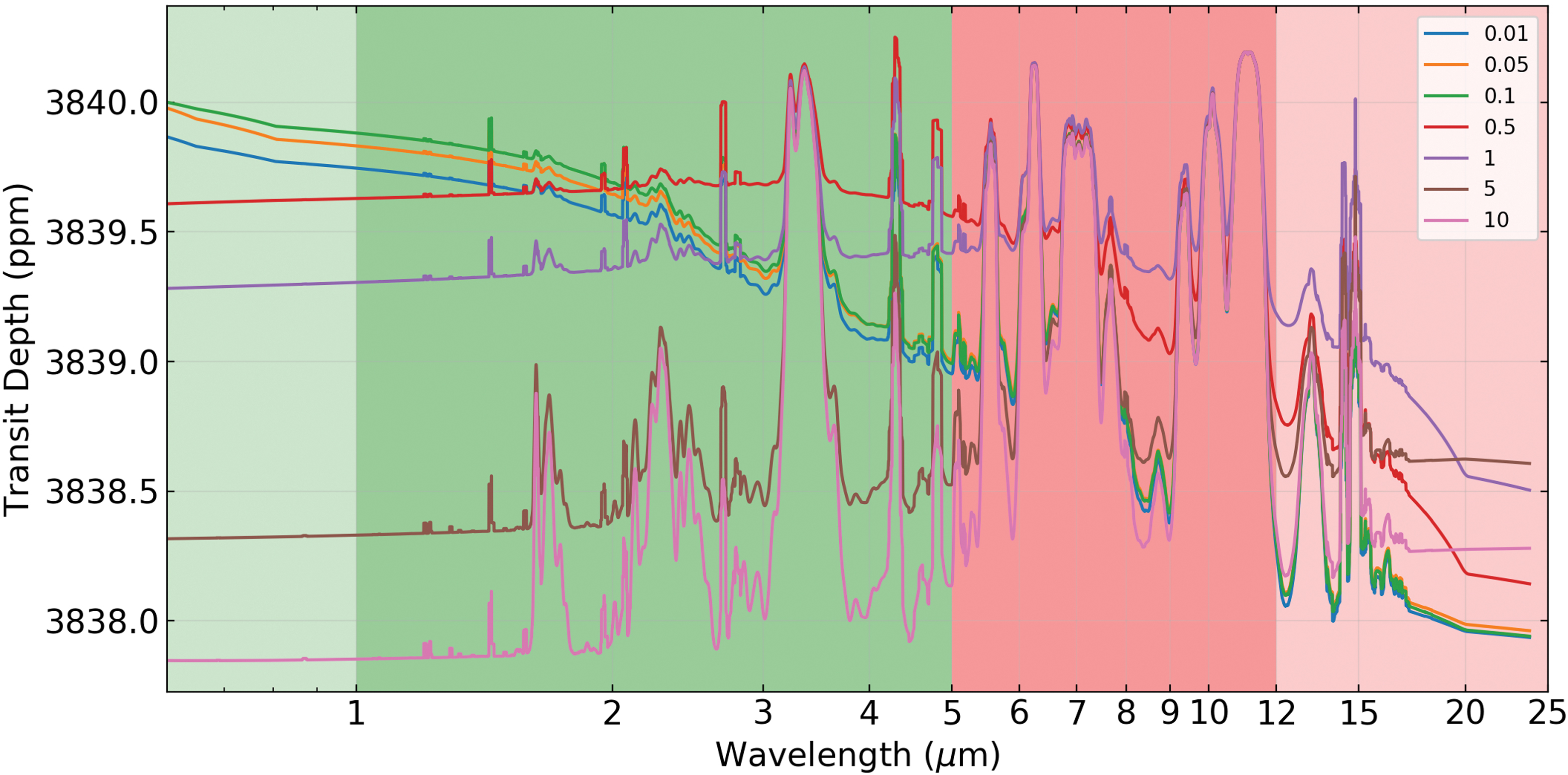
Haze abundance effects on simulated transmission spectra demonstrated using a CO2-dominated atmosphere with an isoprene surface flux of 1 × 10¹³ molecules/(cm2·s) for a habitable super Earth transiting an M dwarf star. The axes are transit depth (ppm) versus wavelength (μm). The isoprene-induced haze size distribution is a Gaussian distribution with mean of 89 nm and standard deviation of 25 nm, and it is approximated from the 10,000 × metallicity, 300 K scenario as described in the work of Hörst et al. (2018). The refractive index proxy for isoprene is C2H2 (Dalzell and Sarofim, 1969). The different colored curves show the simulated transmission spectra as a function of haze/isoprene mass ratio from 1 × 10⁻⁶ to 1. Color images are available online.
For context, the haze-to-methane mass ratio on Titan is ∼0.1 at the thickest part of the haze layer at 400 km altitude. The number density of methane at the same altitude is 1012 molecule/cm3 and the number density around 108 particles/cm3 assuming the particles are 12.5 nm spheres (Fan et al. (2019) and using Titan tholin refractive indexes from the work of Khare et al. (1984). Although it is debatable whether habitable exoplanet atmospheres commonly attain the same abundance of haze as that of Titan, we adopt the haze-to-isoprene mass ratio of 0.1 as the upper bound.
Both experiments and models show that the mean radius of haze particles at standard temperature and pressure are 0.1 micron or smaller (He et al., 2018; Hörst et al., 2018), a particle size that affects shorter (i.e., visible to near-infrared) rather than longer (i.e., mid-infrared) wavelengths. This effect is well known from Mie theory, and it includes the point that once a particle radius is much smaller than the wavelength of light, scattering is in the Rayleigh regime and scales with wavelength as λ−4. We study how different haze particle size affects simulated transmission spectra by using the same inputs as for the haze-to-mass ratio study depicted earlier and shown in Fig. 14. We set the haze-to-isoprene mass ratio to 0.01 and vary the mean particle radius from 0.01 to 10 microns.
For completeness, we explore the effect of mean particle size on the extinction cross-section for a size of 0.01–10 microns. We found that the haze extinction cross-section does not scale linearly with the size of the haze particles when assuming a fixed haze-to-isoprene mass ratio (total mass is constant). Taking Mie theory into account, the maximum strength for the extinction cross-section is for a mean particle size of 0.1 micron (for shorter wavelength) to 1.0 microns (for longer wavelength). For a haze particle size smaller than 0.1 micron, increasing the particle size increases the total extinction cross-section. Overall, different mean particle size will hinder or mask detection of different part of the spectra and is shown in more detail in Fig. 15.
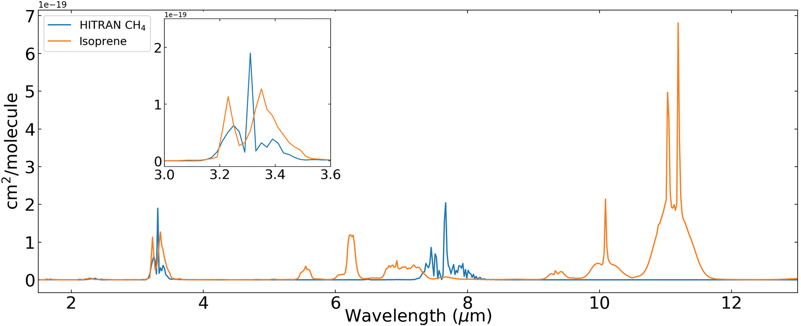
Haze abundance effects on simulated transmission spectra demonstrated by using a CO2-dominated atmosphere with an isoprene surface flux of 1 × 10¹³ molecules/(cm2·s) for a habitable super Earth transiting an M dwarf star. The haze/isoprene mass ratio of this simulation is set to 0.01, and the refractive index proxy for isoprene is C2H2 (Dalzell and Sarofim, 1969). The different colored curves show the simulated transmission spectra with varying haze mean particle size. Changes in the broad-band attenuation and spectral attenuation are not linear with an increase in the mean particle radius. Color images are available online.
Finally, we examine whether different types of refractive indices (as a proxy for haze particle composition) will impact detection. Based on the four types of materials we considered [Titan tholins (Khare et al., 1984), HCN (Khare et al., 1994), C2H2 (Dalzell and Sarofim, 1969), and octane (Anderson, 2000)], we found that although there are minor differences in wavelength-dependent opacities, none of these have unique absorption features that will hinder or mask isoprene spectral features.
4.4. Lack of isoprene false positives
On Earth, isoprene is exclusively produced by life (Section 2.2). Even so, one might suggest that isoprene could be formed geochemically, as a geological false positive, by reduction of carbon dioxide, by reduction of carbon monoxide, or by hydrogenation or dehydrogenation of hydrocarbons. However, the geochemical formation of isoprene on temperate, rocky planets is thermodynamically disfavored (Table 3). For any of the proposed isoprene formation reaction pathways, given the gas concentrations in terrestrial volcanoes, the calculated energy of formation of isoprene makes any geochemical formation scenario very unlikely (a positive Gibbs free energy (ΔG) means the reaction requires energy) (Table 3).
Proposed Geochemical Isoprene Formation Pathways and Energy of Formation of Isoprene from Plausible Geochemical Volatile Concentrations
ΔG is the free energy of reaction at 298 K assuming typical geochemical concentrations of H2O, CO, CO2, CH4, and H2 and 1 ppm isoprene. Average fractions of “wet” gas from magmatic and hydrothermal volcanic systems from the ASM database (Bains et al., 2017): H2 = 0.0028, H2O = 0.9223, CO = 0.000615, CO2 = 0.05332, CH4 = 4.206 × 10⁻⁵. Nonbiological formation of isoprene from any terrestrial geological source is very unlikely for any of the proposed reaction pathways (positive ΔG).
C5H8 = isoprene.
Molecules in a planetary atmosphere may potentially originate from several common abiotic sources, including: the interstellar medium (ISM); as leftover from planetary formation; meteorites and comets; photochemical processes in upper planetary atmospheres; and geological processes on planetary surfaces. None of these processes or environments can efficiently abiotically produce isoprene, as detailed later.
Isoprene and other hydrocarbons containing conjugated double bonds are not known to be a product of ISM chemistry (Ehrenfreund and Cami, 2010; McBride et al., 2013) and are not identified among known ISM molecules (McElroy et al., 2013). We note, however, that many other hydrocarbons, including unsaturated ones, have been detected in ISM (e.g., CH, C2H, CH2, CH3, CH4, C4H, C5H, C6H, C6H2, C6H6, as reviewed by McElroy et al., 2013). Similarly, isoprene and other hydrocarbons containing conjugated double bonds are not detected in meteorites, including in the Murchison meteorite (Levy et al., 1973; Sephton, 2004; Pizzarello and Shock, 2010), a meteorite famous for containing structurally diverse types of organic chemicals.
Photochemical processes in upper planetary atmospheres are also known to not produce isoprene. §§ For example, isoprene and other complex hydrocarbons containing conjugated double bonds are not known to be produced in the atmosphere of Titan. Moreover, the simplest conjugated double bond hydrocarbon (1,3-butadiene) is also not likely to be formed abiotically. Limited theoretical work suggests that nonbiological production of 1,3-butadiene in Titan's atmosphere is, in principle, possible via photochemical reactions, although the rate of formation of 1,3-butadiene is predicted to be negligible. Indeed, so far 1,3-butadiene has not been detected on Titan (Newby et al., 2007) and would likely condense onto haze given the low temperature of Titan. On the other hand, photochemical processes in Titan's atmosphere may lead to the formation of many unsaturated hydrocarbons (e.g., C2H2, ethylene [C2H4], C4H2, C6H2, C6H6 etc.), none of which contain conjugated double bonds (Yung et al., 1984; Maltagliati et al., 2015).
The lack of chemical pathways leading to the abiotic formation of isoprene in a diverse host of planetary environments was recently strengthened by a series of photochemical laboratory experiments on the formation of various gases, including hydrocarbons. The exposure of various mixtures of basic gases such as H2O, CO2, CH4, and NH3 to UV light or plasma at various temperatures in simulated atmospheric scenarios did not show isoprene formation (nor any precursor hydrocarbons to isoprene's formation, nor any other conjugated dienes) (He et al., 2019).
We conclude that isoprene has no known false positive sources. Consequently, its detection in an exoplanet atmosphere would be a strong indication of biological activity.
5. Discussion
We evaluated the candidacy of isoprene as a potential biosignature gas based on the principle that an ideal biosignature gas should satisfy all the following criteria: (1) is produced by life; (2) lacks abiotic false positives; (3) can accumulate to a detectable abundance in exoplanet atmospheres; and (4) has distinguishable spectral features. We have shown that isoprene satisfies the first two criteria (Sections 2 and 4). Isoprene satisfies the first and second criteria but can only satisfy the third and fourth criteria in some scenarios. Therefore, we consider isoprene as a good biosignature gas. Here, we discuss several factors limiting our analysis (Section 5.1), as well as the ability to distinguish isoprene from other hydrocarbons (Section 5.2). We end the discussion by exploring isoprene's ubiquity in many life-forms, and we introduce the concept of isoprene as a “Biosphere Signature” (Section 5.3).
5.1. Limitations of reference data
Our assessment of isoprene as a biosignature gas is constrained by the limited availability of spectral data, our incomplete understanding of isoprene chemistry in anoxic atmospheres, and unknown but potential haze formation from isoprene in anoxic atmospheres. Here, we discuss these limitations and how they may affect our assessment.
5.1.1. Limitations with using absorption cross-sections from lab-measured spectra
Using cross-sections calculated from lab-measured data “as is” without estimating uncertainties for high isoprene mixing ratios can result in atmospheric spectra that are saturated and show artificially strong, wide, and featureless absorption bands (see Supplementary Appendix Fig. A4), which lead to inconclusive detection predictions. This effect is unphysical, because in some wavelength ranges, the true cross-section values are likely much smaller than the instrumental noise floor. The Brauer et al. (2014) wavelength-independent uncertainty is approximately four orders of magnitude weaker than the strongest absorption peaks of isoprene. Based on Beer-lambert law, for transmission spectroscopy, the cross-section uncertainty will also need to be eight orders of magnitude weaker than the strongest absorption peaks to avoid the unphysical effect. Therefore, we recommend future lab-based measurements of the isoprene cross-sections to focus on measuring the strength of the weak absorption features, or location of the spectra where there are no spectral peaks, so that it is possible to differentiate between real, but weak transitions and the noise floor.
A possible work-around method is to subtract the uncertainties from the data, leaving only the strongest peaks. However, we disfavor discarding cross-section values below an arbitrary value because it can remove weak, but real, absorption lines. Although individually these weak lines are negligible, collectively they can drastically change the overall opacity, and subsequently conclusions on the potential for detection. We show in Supplementary Appendix Fig. A4 how such an unphysical noise floor cut-off can artificially remove the weak features of isoprene and re-engineer the spectrum and associated detectability of isoprene.
In addition, we encourage the measurement of isoprene spectra to cover a broad temperature/pressure range relevant for exoplanet atmospheres. A broader coverage as compared with the current standard temperature and pressure measurements would allow extrapolation of isoprene cross-sections to conditions that are more appropriate for the upper atmosphere of a variety of exoplanets. Calculating molecular line lists by using ab initio theoretical quantum mechanical methods is computationally demanding (e.g., Tennyson and Yurchenko, 2012), often requiring years of work even for a small molecule, and it is not currently possible to obtain accurate theoretical cross-sections for isoprene due to the complexity of the molecule (see Sousa-Silva et al., 2019 for a more in-depth discussion on alternatives). However, we emphasize that our SEAS model is sufficiently versatile to be able to quickly update its predictions on isoprene detectability whenever improved cross-sections for isoprene become available.
5.1.2. Limitations to isoprene reaction rates
In this work, we have only focused on the reaction of isoprene with UV and the dominant radical species O⋅ and ⋅OH. The photochemistry of isoprene with other, potentially relevant radicals, such as H⋅, Cl⋅, and ⋅CnHm is insufficiently studied. Inclusion of these radicals may potentially increase the isoprene destruction rate. Our models may not include all chemical reactions that are relevant to anoxic, temperate terrestrial planets. Therefore, more detailed studies of anoxic atmospheric chemical reaction networks are required.
Many M dwarf stars have frequent, strong flares. Flares introduce intense packets of UV radiation capable of destroying biosignature gases, including isoprene (Segura et al., 2010; Tilley et al., 2019). Recent work by Günther et al. (2019) has found 30% of late M dwarf stars and 5% of early M dwarf stars display active flaring events. Future photochemistry models, therefore, will require consideration of flaring activities and addressing how flaring activities impact habitability and accumulation of biosignature gases.
5.1.3. Limitations to understanding isoprene induced haze
No one has yet addressed the formation of isoprene-induced hazes in anoxic planetary atmospheres. On Earth, isoprene destruction rapidly leads to haze formation. Further studies on constraining the isoprene-haze mass ratio and mean particle size in anoxic planetary atmospheres are needed because sub-micron haze particles can heavily mute transmission spectral features at wavelengths up to 4 μm, as demonstrated in Section 4.3.
In addition, high-altitude hazes in an anoxic atmosphere could act as a UV shielding mechanism for biosignature gases, therefore increasing the probability of their accumulation (Segura et al., 2005; Seager et al., 2013).
5.2. Isoprene spectral distinguishability versus other hydrocarbons
In addition to isoprene and methane, all hydrocarbons have spectral features at 3.1–3.7 μm, due to the C-H bond stretching rovibrational band, and many have spectral features at 9–12 μm, due to the C-H bond bending rovibrational band. Figure 16 shows a comparison of isoprene with methane and other simple hydrocarbons that highlights the challenges in the unambiguous identification of isoprene. Though isoprene accounts for most of the non-methane hydrocarbons released by life on modern Earth (Sharkey et al., 2008), simpler hydrocarbons have more favorable abiotic formation pathways, which may lead to their accumulation in the atmosphere. Therefore, we need to study isoprene distinguishability in the context of other hydrocarbons that may be readily present in the atmosphere.

Isoprene (red) and methane (green) versus 80 other hydrocarbon (grey) absorbances. The axes show absorbance (normalized to 1) versus wavelength (μm). The hydrocarbon absorbance data are taken from NIST lab-based measurements and include all hydrocarbons, with fewer than seven carbon atoms that have spectral measurements. Due to measurements being made with different instruments and experimental set-ups, we normalize the absorbances to one for a qualitative comparison. We show that although isoprene has many broad spectral features, it does not stand out when comparing with the collective sum of spectral features from other hydrocarbons. Therefore, it is possible for a coincidental combination of simple hydrocarbons to mimic isoprene spectral features. Color images are available online.
The 3.1–3.7 μm features are the C-H bond stretching vibration features and can have three main functional groups: carbon single bonds (X-C-H) located at 3.45 μm, carbon double bonds (X = C-H) located at 3.23 μm, and carbon triple bonds (X#C-H) located at 3.03 μm (X denotes a non-hydrogen atom bonded to the carbon atom; see Section 3.1.2 for more details on these features). For molecules that have only one spectrally active functional group, distinguishing between molecules within each group requires a spectral resolution of at least R = 200. Fortunately, isoprene has both the (X-C-H) bond and the (X = C-H) bond, so detection of its 3.1–3.7 μm can be done with a spectral resolution of R = 20. We note, however, that a coincidental mixture of simple hydrocarbon molecules in the atmosphere can mimic the isoprene spectral features at 3.1–3.7 μm. For example, an equal amount of ethane (C2H6), which only contains the (X-C-H) bond, and C2H4, which contains only the (X = C-H) bond, would be indistinguishable from isoprene if observed at low resolutions. We additionally note that hydrocarbons containing the isoprene substructure can also mimic isoprene spectral features.
The isoprene spectral features at 9–12 μm are due to the vibrational bending of the C-H bond, and many contain many rovibrational substructures. Distinguishing isoprene from other hydrocarbon molecules in this spectral region can be challenging. Recent work by Sousa-Silva et al. (2019) developed a computational tool (RASCALL: Rapid Approximate Spectral Calculations for ALL) to estimate spectral data (position in the spectra and relative strength) for any molecule by combining functional group data from experimental measurements, organic chemistry, and quantum mechanics; these methods can aid in identifying which molecules struggle to be distinguished from one another, and they highlight the issues surrounding the distinguishability of isoprene from other hydrocarbons.
5.3. Isoprene as a “biosphere signature”
Isoprene stands out among the studied biosignature gases not only because it is produced in high abundance by life on the Earth but may also be due to isoprenoid biosynthetic pathways, which are responsible for synthesis of isoprene and many other terpenoids; these are present in virtually every domain of life on Earth, that is, Bacteria, Archaea, and Eukarya (see Section A2.2 in Supplementary Appendix A2). Although the synthesis and likely functions of isoprene on Earth are closely linked to oxygenic photosynthesis in plants, many non-photosynthesizing organisms make isoprene, and its synthesis is not dependent on an oxygenated atmosphere. It is plausible, therefore, to speculate that an entirely anaerobic biosphere could produce high levels of isoprene.
Even if isoprene itself is not made by every species on Earth, a wide variety of molecules that contain the isoprene-motif, or isoprenoids, are created. The isoprene motif and its structural derivatives are utilized to synthesize countless chemicals in all of Earth's life. In contrast to previously proposed classical type III biosignatures such as methyl chloride, methyl sulfide, and DMS, isoprenoids have a much larger coverage of the phylogenetic tree of life (Seager et al., 2012).
Isoprenoids are produced by many evolutionary distant organisms occupying diverse ecological niches (e.g., both marine and terrestrial surface and subsurface environments). Out of other proposed type III biosignature gases, only DMS is produced by a host of evolutionarily diverse organisms but nowhere near to the phylogenetic diversity of isoprenoid production. Other frequently cited type III biosignatures (such as N2O and CH3Cl) are produced by less diverse species. In addition, all of them inhabit very similar habitats (e.g., methyl chloride is released mainly by several species of marine algae and to a lesser extent by the soil bacteria and fungi; 62% of the global N2O emissions is produced by nitrifying and denitrifying bacteria and fungi in the soil; Maeda et al., 2015). Isoprene and other isoprenoids do not have these limitations. Therefore, isoprene is the most widely made molecule, yet it is evaluated as a biosignature gas. Moreover, there are at least two distinct isoprenoid biosynthesis pathways, and isoprene synthesis likely has evolved independently multiple times so it is plausible to suggest that it might evolve in other worlds. Therefore, we postulate that isoprene and other volatile isoprenoids could be considered characteristic, unifying chemical signatures, specific and common to the whole Earth-type biosphere. In essence, isoprenoids are more than biosignatures—they are “biosphere signatures”—chemicals that are a molecular fingerprint of the entire Earth-type biosphere.
Footnotes
Acknowledgments
The authors thank Mihkel Pajusalu, Karen Cady-Pereira, Robert Hargreaves, and Iouli Gordon, for lengthy discussions on using molecular absorption cross-sections calculated from lab-measured spectra for exoplanet atmosphere simulations. They also thank Thomas Evans, Jason Eastman, Elisabeth Matthews, and the Seager group for helping them to establish the detection metric. Finally, they thank Joanna Petkowska for contributing Figs. 2 and ![]() .
.
Author Disclosure Statement
No competing financial interests exist.
Funding Information
The authors thank the MIT BOSE Fellow program, the Change Happens Foundation, the Heising-Simons Foundation, and NASA grants 80NSSC19K0471 and NNX15AC86G for partial funding of this work. S.R. gratefully acknowledges support from the Simons Foundation, grant number 495062.
Supplementary Appendices
Supplementary Appendix A1. Atmospheric Mixing Ratios and Temperature-Pressure Profiles
Supplementary Appendix Fig. A1
Supplementary Appendix Fig. A2
Supplementary Appendix Fig. A3
Supplementary Appendix Fig. A4
Supplementary Appendix A2. Structural Diversity and Biosynthesis of Isoprenoids
Supplementary Appendix Fig. A5
Supplementary Appendix Fig. A6
Supplementary Appendix Table A1
Abbreviations Used
References
Supplementary Material
Please find the following supplemental material available below.
For Open Access articles published under a Creative Commons License, all supplemental material carries the same license as the article it is associated with.
For non-Open Access articles published, all supplemental material carries a non-exclusive license, and permission requests for re-use of supplemental material or any part of supplemental material shall be sent directly to the copyright owner as specified in the copyright notice associated with the article.