Analysis of Early Iron Sulfide,Carbonate,and Phosphate Mineral Analogues Produced by Flow-Driven Precipitation in a Microchannel

Abstract

Most of the chemical and physical interactions of interest to the astrobiology community are influenced by the mineralogy of the systems under consideration. Often, this mineralogy occurs in sediment or sediment-like aqueous microenvironments in which the early minerals differ dramatically from the mature version that results from a long diagenesis, which are tied to complex interactions of pH, redox state, concentration, and temperature. This interconnectedness is difficult to reproduce in a laboratory setting yet is essential to understanding how the physical and chemical demands of living systems alter and are altered by their geological context. We present a facile means for producing precipitated mineral analogues within a microchannel and demonstrate its analytical efficacy through instrumental and modeling techniques. We show that amorphous, early-stage analogues of iron sulfide, iron carbonate, and iron phosphate can be formed at the boundary between flowing solutions, modeled on the microscale, and analyzed by standard instrumental techniques such as scanning electron microscopy/energy-dispersive spectroscopy, X-ray photoelectron spectroscopy, and Raman spectroscopy.

1. Introduction

The chemistry of natural systems is draped over the landscape of the physical world. This is a problem for fields such as astrobiology, paleogeology, and origins of life research that do not have access to the physical world under study because of its physical or temporal distance. In planetary systems, redox gradients, temperature, pressure, concentration trends, flow profiles, and time conspire to produce geochemistry, and even within a single planetary system individual environments can be difficult to characterize. In the case of Earth, life has so fundamentally altered the mineralogical (Hazen et al., 2008) and energy (National Research Council, 2019) landscape of our planet that using its geochemistry as a foundation for other worlds past and present may be misleading.

The energy and chemical activity of living systems have a fundamental impact on basic science questions of erosion and sedimentation (Montague, 1986), redox gradients in the geological record (Jin et al., 2016; Zhang et al., 2019), and metal concentrations (Davranche et al., 2020) that inform systems of ancient (putatively) lacustrine systems on Mars (Horgan et al., 2020).

This presents a problem for synthesizing diverse research in the context of the many plausible natural conditions that can be imagined for any particular geochemical environment. On the one hand, it is the excellent work of researchers showing that colloids and phospholipids are driven by the gradients mentioned above into iron sulfide precipitates (Möller et al., 2017), that temperature gradients can accrue large excesses of biomolecules (Baaske et al., 2007), that proton gradients can themselves be the result of temperature differences across micropores (Keil et al., 2017), and that such gradients may have something to do with how abiogenesis is powered (Lane, 2017; Bonfio et al., 2018).

On the other hand, it is the physical world over which these chemistries may have been draped, which may preserve (Tan and Sephton, 2020), enhance (Mielke et al., 2011), or degrade (Jackson, 2016; Liu and Kounaves, 2021) these phenomena depending on small changes to the real-world conditions. Every warm little pond has a bottom, and the physical and chemical interactions between a natural system and its mineral boundaries can drive an enormous range of plausible conditions for constraining experiment and theory.

The early digenesis of precipitated minerals represents the time when the physical and chemical state of the system is in greatest flux and consequently a time in which the effect of biological or protobiological systems are expected to produce chemical and thermodynamic changes to the nascent mineral's maturation. Mature mineralization produces profound changes to the mineral's physical and chemical state, and it is unclear how the deposition and diagenetic fate of minerals such as iron carbonates known to exist in sites of interest to the astrobiology community (Brown et al., 2020; Horgan et al., 2020) are altered by the presence of living organic matter in comparison with abiotic organic matter or an absence of organic material.

For example, even if explicit biosignatures of living systems are absent in the apparently fluvial deposits of Mars' Jezero Crater, does a lasting impression of their presence linger in the otherwise inorganic mineralogy of the iron minerals that are extant? Put another way, what does fluvial mineralogy look like in the absence of living or abiotic organic matter? What is needed (in our view) is a robust framework for producing and analyzing mineral analogues within the kinds of pH, redox, and flow gradients that are endemic to natural systems.

We present here a facile method for producing analogues of early precipitated iron minerals within gradients of pH, redox potential, ion concentration, and flow that are analogous to natural conditions. Three iron systems are studied here: Fe(II)-sulfide, Fe(II)-carbonate, and Fe(II)-phosphate. A total of 1–5 mM FeCl₂ meets 1–5 mM Na₂S, Na₂CO₃, or Na₂HPO₄ at a solution–solution boundary in a microchannel, and precipitate at that junction accretes to form the mineral analogue. Fe(II) is chosen for its ubiquity in natural environments, role in microbial metabolism, and putative role in early life on Earth.

The anions sulfide, carbonate, and phosphate were also chosen not only for their ubiquity, but also for the ubiquity of their incorporation into iron minerals of current interest to the astrobiology community (Horgan et al., 2020). We leverage scanning electron microscopy (SEM), energy-dispersive spectroscopy (EDS/EDX), X-ray photoelectron spectroscopy (XPS), and Raman spectroscopy as well as a purpose-built channel model and image analyses to characterize the evolution and fate of the mineral analogues produced.

The analysis techniques applied and the material to which they are applied are of equal scientific importance in our view. Taken together, these methods represent a cohesive framework for studying complex questions of mineral–water interactions of principle importance to the origins of life and planetary science communities. The flexibility of the instrumental and numerical modeling analysis described here allows for application to a range of other chemical systems and science objectives related to aqueous formation of geologically relevant material, its weathering, and the influence of factors such as organic content and speciation on geochemical outcomes.

2. Materials and Methods

2.1. Reagents

All reagents were used as received except where noted. Solutions were prepared by adding degassed, deionized water (18 MΩ) to FeCl₂·4H₂O (Sigma-Aldrich), Na₂CO₃ (Sigma-Aldrich), Na₂S · 9H₂O (Sigma-Aldrich), Na₂HPO₄ (Sigma-Aldrich). These solutions were then transferred to 50 mL Falcon tubes capped with rubber septa (Nsil Lab Glass Works). Solutions were placed under low vacuum by manually withdrawing the air within the tube in a 500 cc syringe with an 18g needle. A small flow of N₂ (airgas, 99%) was introduced until pressurization of the tube occurred, and then a constant flow was produced by inserting a second vent needle. These two steps (vacuum and vent) were repeated twice in sequence.

A constant flow of ∼1 psig of N₂ was then maintained until solutions were used, with all solutions being prepared and used within 4 h of degassing. A supply of partially deoxygenated, deionized water for flushing was provided in the same manner before each experiment, with the same used as the makeup water for solutions as described above. A brief explanation of the method development for this degassing procedure and its role in experimental design can be found in the Supplementary Data, section 1.1.

2.2. Microdevice fabrication

2.2.1. Mold-cast microdevice

A Y-channel microdevice (Fig. 1) was fabricated using standard photolithographic techniques (Lee and Sundararajan, 2010). In brief, a CAD design of the chip was used by CAD/Art Services, Inc. (Bandon, OR) to create an ink-on-polymer mask. This mask was used to expose a photoresist (SU-8), which hardens into a negative mold, ∼70 μm tall, of the CAD design. Polydimethylsiloxane (PDMS) monomer and curing agent were mixed in a 10:1 ratio, poured over the positive mold, and allowed to cure overnight at 80°C.

FIG. 1.

(Left, top) The microdevice used in this work is a single Y-channel, 70 × 500 μm in cross-sectional aspect and 15 mm long. (Left, bottom left) The microdevice is compressed between two glass slides, with the typical orientation viewing the channel through one of these slides, which acts as the channel ceiling. (Left, bottom right) Producing material directly onto conductive substrates such Au-coated glass or high-purity Al foil is useful for some analysis techniques, and in these cases a “flipped” orientation is used in which the timelapse images are taken through the optically transparent PDMS, and the typical conductive Au or Al is the channel “floor.” (Right) In either orientation, a 700 × digital microscope images the experiments. PDMS, polydimethylsiloxane.

The final channel dimensions were 70 μm tall × 500 μm wide, with the straight region where membrane formation occurs being 1.5 cm long. Inlet and outlet wells (referred to as vias here) were created by removing material perpendicular to the channel (circular region) with a 2 mm biopsy punch. Through-holes were then biopsy-punched orthogonally between the 2 mm vias and the outside of the PDMS to facilitate fluid line insertion when the microdevice is compressed within the experimental stage.

2.3. Microdevice preparation

Because access to the channel is necessary postexperiment to analyze the material produced, the PDMS microdevices and glass substrate were not irreversibly bonded as is typical in microfluidics (Benhabib et al., 2010; Kim et al., 2016). The microdevices were instead cleaned with isopropyl alcohol (IPA) and pressed onto a similarly cleaned glass slide, Au-sputtered glass slide, or high-purity Al foil (Shop Aid). The microfluidic unit at this point consisted of two glass slides with the patterned PDMS sandwiched between (Fig. 1). Using the two glass slides as rigid supports, polytetrafluoroethylene (PTFE) tubing (0.023″ ID) was inserted into the 1 mm holes punched earlier in the PDMS. This unit was then placed between an acrylic compression plate and aluminum block, and four screws were hand tightened just until resistance was encountered.

2.4. Experimental setup

A KD Scientific syringe pump (Legato 180) was fitted with two 15 cc syringes filled with degassed, deionized water (ddH₂O) prepared above. Microfluidic devices were then flushed and checked for leaks before each experiment, and ddH₂O syringes replaced with reagent syringes. Unless otherwise noted, experimental concentrations are assumed to be equimolar (i.e., 1 mM FeCl₂ to 1 mM Na₂S). A 600–900 × digital microscope (Dino-Lite) was positioned above the channel of the microdevice, and 5-s timelapse images were collected for the duration of the experiment using Dino-Lite software (Dino-Lite 2.0).

Each combination of flow rate, Fe(II) concentration, anion concentration, and anion species was repeated at least twice. After each experiment, N₂ was used to clear the majority of the fluid from the microdevice. The slide not in contact with the channel was removed from the PDMS microdevice's back, and the device was placed under a 5 psig flow of N₂ in a septa-capped Falcon tube for ∼20 min until fluid droplets were no longer visible at channel wells and stored under a back-pressure of N₂.

2.5. Sample preparation and instrumental analysis

After membrane formation and drying under N₂, the glass substrate and PDMS were carefully separated, enabling analysis of precipitated material adhered to these individual halves of the microdevice. For SEM/EDS results shown here, material was transferred from the slide/foil or PDMS to double-slided carbon tape on an SEM stub by careful rolling contact. All analyses were performed on both glass and aluminum devices; however, SEM/EDS results are exclusively Au-sputtered glass slides or aluminum foil mounted with carbon tape to standard SEM pin mounts due to charge-limited signal intensity on glass slides. EDS signal is greatly enhanced by conductive backplane in these cases.

A Thermo K-alpha XPS was used with Ar flood gun and a spot size of 400 μm. Survey spectra were taken with 0.5 eV step size, while detailed elemental peaks were characterized with 0.1 eV step sizes. Peak analysis was done using Avantage software (v5.938).

A Thermo Nicolet Almega XR Dispersive Raman Spectrometer was used with a 488 nm laser and 20 × , 50 × , and 100 × objectives. All spectra were taken under 100 × objective at a laser power of 0.1–5% (1.5–4 mW). Laser power was adjusted to minimize sample heating. A typical spectrum consisted of 250 scans (∼90 s). Spectra were processed with Origin (v9), OMNIC (v8), and CrystalSleuth (v2008) with the RRUFF database. Major peak assignments were also done manually by comparing with published results cited here and furnished through the web interface of the RRUFF project.

SEM was accomplished with a Zeiss Ultra 60 at accelerating voltages of between 5 and 15 kV. A coupled EDS was used with AzTec (v3.0) to derive elemental localization and relative abundance.

2.6. Image analysis

Timelapse images from the 700 × camera are converted to grayscale, and low-albedo pixels are counted based on a binary threshold (values darker than the threshold = 1, all lighter values = 0). A pixel-to-distance conversion is calculated based on the known channel dimension and pixel measure between channel walls. These counts were processed in Python 3.9 with several libraries. A detailed description of image processing and code information can be found in the Supplementary Data, section 1.2.

2.7. Flow and diffusion modeling

A channel model was produced in Python 3.9 with libraries and details as described in Supplementary Data, section 1.3. In brief, a flow velocity profile is solved assuming a no-slip boundary condition, and this profile is used to numerically simulate diffusion of each chemical species in the channel. The model assumes a rectangular channel cross-section with arbitrary wall geometry (i.e., any wall-like boundary within the rectangular cross-section can be specified and flow equilibrated for the new boundary). Each of the two reactant solutions is assumed to initially flow freely where they meet at the channel centerline (full-slip condition), and only diffusional mixing of reactants at this laminar flow boundary is calculated.

3. Results

3.1. Precipitates observation, timelapse image, and morphology

In all cases, precipitation is visible within the first few seconds of reactants entering the microchannel. Throughout this work each FeCl₂-Anion system will be referred to as “Fe(II)-anion.” For example, the precipitate that forms at the boundary of FeCl₂ and Na₂HPO₄ solutions will be referred to as “Fe(II)-phosphate precipitate.” This convention is an attempt to maintain clarity in discussion of the observations of material formation and characterization, with more formal stoichiometric analysis formatted as typical chemical formulae [i.e., “FePO₄,” “iron(III) phosphate”].

Figure 2 illustrates some characteristic examples of each chemical system. Fe(II)-sulfide and Fe(II)-carbonate systems grow quickly and plateau, following the same general trend. Fe(II)-phosphate, on the contrary, continues to grow laterally over the course of the experiment. Mean material accretion rates were not significantly different between 50, 100, and 200 μL/min flow rates for Fe(II)-sulfide and Fe(II)-carbonate systems; however, Fe(II)-phosphate exhibits flow-dependent rates throughout the first few minutes of precipitate formation (Supplementary Data, section 3). The differences in color within the first few minutes of precipitation are striking, and in the case of the Fe(II)-phosphate system this color banding highlights steep gradients of pH, redox potential, and ionic species that exist at the laminar boundary between two flowing systems on the microscale.

FIG. 2.

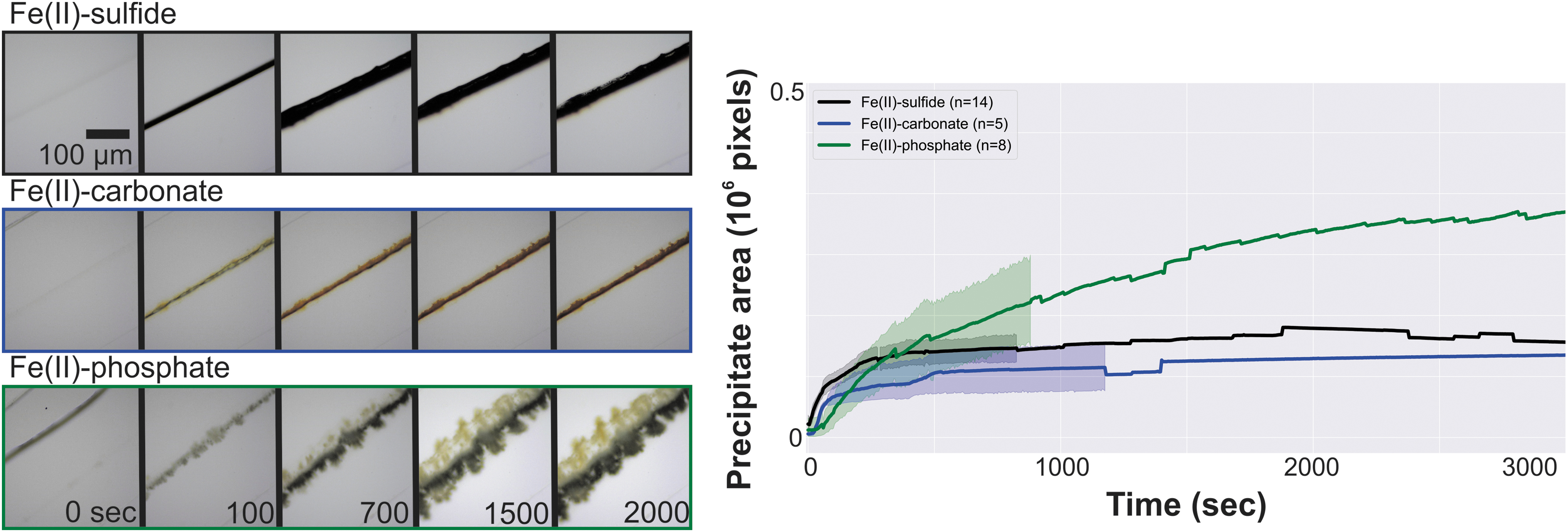
(Left) Timelapse images of representative mineral analog accretion for Fe(II)-sulfide, Fe(II)-carbonate, and Fe(II)-phosphate systems. (Right) Broad trends in accretion profile are highlighted by plotting average precipitation area over time for experiments from 1 to 5 mM in both reactants at flow rates of 50, 100, or 200 μL/min. Fe(II)-phosphate accretion continues for the duration of the experiment, while both of the other systems reach a stable plateau. All images are at the same scale. Shaded regions are 95% CI. CI, confidence interval.

The morphological influence of flow can be seen in SEM micrographs of the Fe(II)-sulfide system, which preserve flow features such as scalloped banding from sequential material deposition as shown in Fig. 3A.1 and B.2. Of particular interest are the dendritic growths surrounding the gap (Fig. 3A.2), where material at the top and bottom of the channel grow toward eventual closure.

FIG. 3.

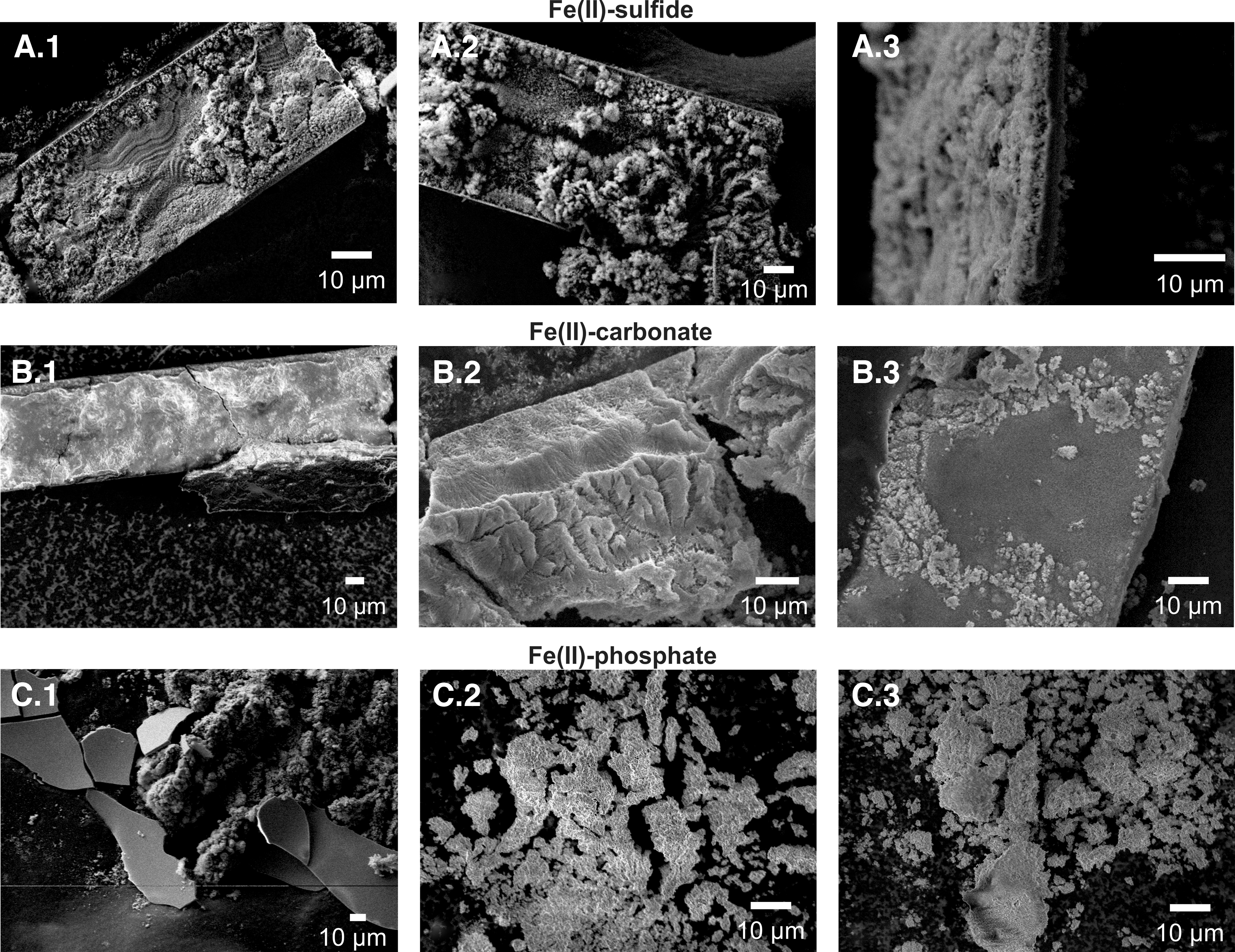
Representative micrographs for each chemical system in this work. Both Fe(II)-carbonate and Fe(II)-sulfide “membranes” are shown side-on in images A.1, A.2, and B.1–B.3. The straight boundaries are the regions that were in contact with the top or bottom of the microchannel. A.3 illustrates how thin and coherent the “membranes” can be; the perspective is top-down and edge-on a particularly thin version. (C.1–C.3) At all scales, Fe(II)-phosphate material is branched, loose, and disordered. (C.1) The exception is regions from the top or bottom of the channel distal to the channel centerline where plated material often forms coherent mats.

Morphological features reminiscent of flow deposition are associated with the likely locations of such accretion closures. A frequent phenomenon observable in most experiments in Fe(II)-sulfide and many Fe(II)-carbonate is the sudden appearance of dendritic outgrowths as the overall growth of material in the channel has begun to plateau. In some cases, these growths deform flow and drive the formation of a second “layer” of material on either side of the previous, centerline material boundary.

This material boundary is always coherent for Fe(II)-sulfide and Fe(II)-carbonate; however, this is not true of the Fe(II)-phosphate material at any scale. The continued growth over the course of the experiment can in part be motivated by the loose, branched structure of the precipitate through which diffusive transport is possible in contrast to the solid boundaries produced by the other two chemical systems.

Oxidation of deposited material occurs over the course of the experiment in some cases. Fe(II)-sulfide will visibly redden after ∼10 min in many cases. A drop in precipitate area is also noticeable in most Fe(II)-sulfide experiments but is difficult to see in Fig. 2 due to scale and averaging. A putative “green rust” formed in 3 of Fe(II)-carbonate experiments reported here as shown in Fig. 4. These species are sandwiched Fe(II)/Fe(III)-hydroxide species with an anion such as carbonate stabilizing interstitial sites, and as such are easily oxidized. Figure 4 (right) shows the oxidation of the Fe(II)-phosphate material over the course of days post experiment. Siderite (FeCO₃) itself can be photo-oxidized (Kim et al., 2013), and it is possible that photo-oxidation of Fe(II) is a feature of some phenomena discussed here (Tabata et al., 2021).

FIG. 4.

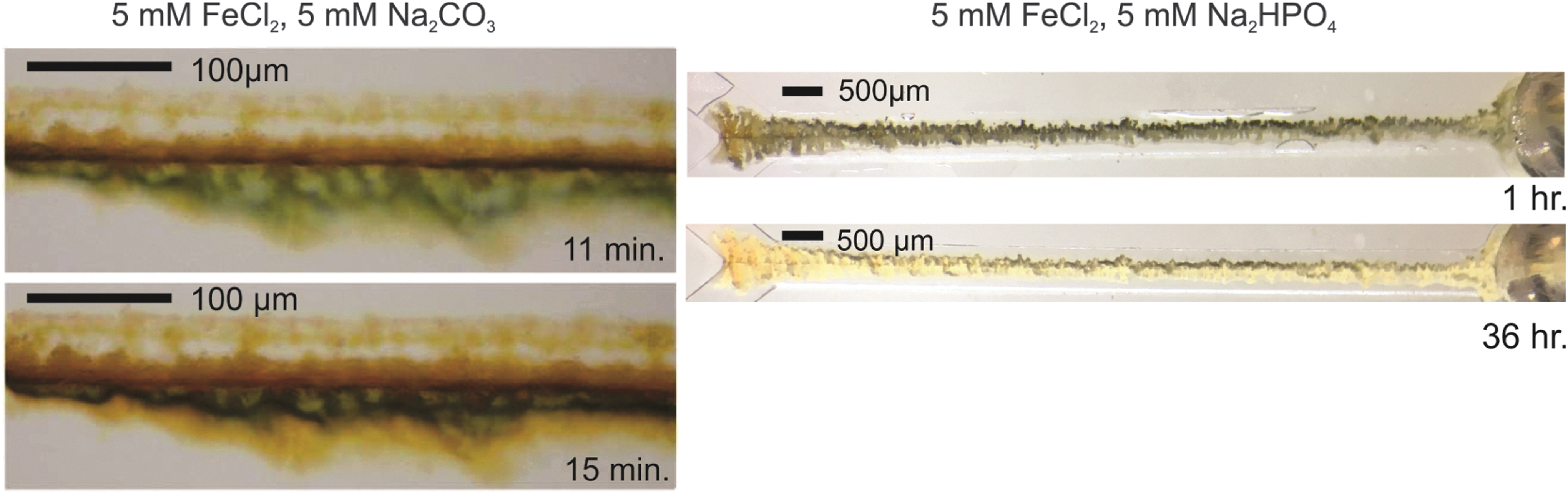
(Left) Possible formation of “green rust,” a mixed Fe(II)/Fe(III) species oxidizes rapidly within the channel. Solutions are anoxic, and this oxidation is likely the result of in place redox displacement reactions. (Right) Fe(II)-phosphate experiments oxidize over the days after formation.

While precipitate formation was not generally observed to occur readily in solutions that were not degassed (Supplementary Data, section 1.1), it is also possible that some of the observed oxidation occurs because of incomplete oxygen removal during degassing. The permeability of oxygen through PDMS is significant, and no attempt was made to minimize its oxidative effect from this source, although anoxic handling and experimental techniques have been used in other work, for example in anaerobic microbial culturing (Dickson, 2019).

3.2. Instrumental analysis

Figure 5 shows selected, representative results from instrumental analysis of the deposited precipitate. The dominant peak assignments in most Raman spectra were iron oxide and iron oxyhydroxide species. This is highlighted by the select spectra of Fig. 5B in which only the broad P-O stretch (Zhang and Brow, 2011) at ∼1000 cm⁻¹ is significantly different. Most spectra were low intensity after 250 scans at the highest laser power, which did not produce fluorescence or the sample destruction, which many of the small features of the samples analyzed here were prone to. In the case where strong peaks did occur, these were assigned to iron oxides and iron oxyhydroxides (Boucherit et al., 1991; De Faria et al., 1997; Hanesch, 2009; Weber et al., 2015).

FIG. 5.

Select Raman spectra for (A) Fe(II)-carbonate and (B) Fe(II)-phosphate show a sampling of low-intensity signal representative of the material analyzed. Note the peak at ∼1000 cm⁻¹ indicative of the P-O stretch of phosphate. (C) XPS spectra of (black) Fe(II)-sulfide, (green) Fe(II)-phosphate, and (blue) Fe(II)-carbonate. Spectra are shown stacked (Raman) and without deconvolved assignments (XPS) to emphasize comparison. Spectra are corrected to Fe(II)-carbonate low BE shoulder. XPS, X-ray photoelectron spectroscopy, BE, binding energy.

Two common features are broad peaks at ∼1300 cm⁻¹ assigned to the asymmetric stretch of either Fe-OH [goethite (α-FeO(OH)) or lepidocrocite (γ-FeO(OH))], or hydrated magnetite and hematite (Fe²⁺Fe₂ ³⁺O₄ ²⁻ and Fe₂ O₃, respectively), and a broad peak between 600 and 700 cm⁻¹ assigned to various Fe-O symmetric stretches associated with magnetite, ferrihydrite [(Fe³⁺)₂O₃·0.5H₂O], and wüstite (FeO). Two primary “types” of iron oxides(hydroxides) are seen: a type with two dominant peaks between 200 and 400 cm⁻¹, and a type with three. In each case these are assigned to different lattice speciations of Fe-O symmetric stretch or asymmetric bend. At ∼400, the final very strong peak (of the 2/3 just mentioned) is assigned to the Fe-O-Fe or Fe-OH symmetric stretch.

XPS analysis of O 1s is shown in Fig. 5C. The O 1s signal is highlighted for two reasons: (1) low signal for Fe 2p, S 2p, and P 2p because of small sample size (small surface area), and (2) oxygen in the form of phosphate and carbonate have strong binding energy shifts. Low signal is due to the small surface area of the monolithic “membranes.” While the spot size of X-rays (400 μm) is adjustable, this adjustment results in an additional net loss of signal as pinhole substitutions are the means of narrowing the beam and these simply block radiation rather than focusing the same intensity into a smaller area. This effect can be seen in the relative increase of Fe(II)-phosphate signal in Fig. 5C as the loose, noncohesive nature of the material produced covers a wider area.

Extensive charging effects were encountered on fresh samples even with the use of an Ar flood gun, likely owing to the high-water content as evidenced by long waits for vacuum chamber pressures to reach the 10⁻⁷ torr ranges required for XPS analysis. For this reason, charge correction has been made to the low binding energy shoulder of the (blue) Fe(II)-carbonate spectra, assigned to a broad contribution from near-surface Fe-O states. C 1s spectra are dominated by carbon mounting tape in all cases. These results are consistent with those reported for other amorphous iron sulfides, iron carbonates (siderite), and iron phosphates (vivianite) (Herbert Jr et al., 1998; Heuer and Stubbins, 1999; Mullet et al., 2002; Wang and Sherwood, 2002).

It is clear from Fig. 5 that phosphorus and carbonate are present; however, Raman spectra are strongly affected by the degree of coordination within a sample (Kailer et al., 1999), and the amorphous nature of the fresh precipitates analyzed here makes them unlikely to be highly coordinated. This is logical, as the number of “forbidden” transitions that give rise to the Stokes spectra measured is small, and a large number of a given chemical state are required to produce enough signal to be visible. For example, Fig. 6 shows a 100 × optical image from which a micro-Raman spectrum has been obtained.

FIG. 6.

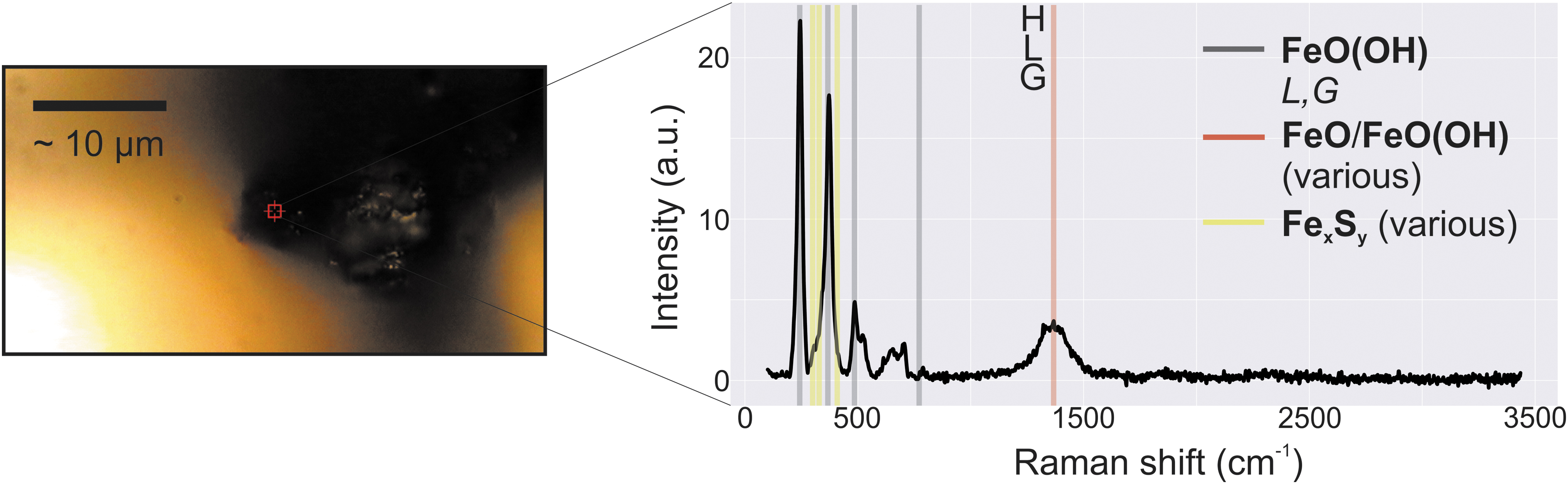
Iron sulfide material is visually distinct, with a dark black coloration that fades over the course of several days. The fresh sample shown in the image and its attendant spectra shows little signal from iron sulfide peaks (each of the dominant expected species have peaks in the yellow regions). Iron oxide and oxyhydroxide dominate instead. This result is consistent with samples that have aged for 24 and 72 h, by which time oxidation is nearly complete. (H) = hematite, (L) = lepidocrocite, (G) = goethite.

The sample is clearly some form of iron sulfide, as the dark black color and a faint odor of “rotten eggs” from evolving H₂S gas attest when the N₂-purged sample container was opened. Sulfidic species are not obvious in the spectra, however, with no strong signals in the yellow regions where they would be expected. The lack of typical diagnostic peaks such as the ∼1080 cm⁻¹ carbonate peak is also not uncommon in amorphous precipitates in small quantities, for example in electrochemical production of green “rust” (Legrand et al., 2001) or thin iron in carbonate solution (Perkins and Garber, 2003).

Sample masses are so small that they are sometimes transparent to Raman spectroscopy as evidenced by spectroscopic peaks related to the Si-O stretch of the glass slide underneath precipitate samples (Supplementary Data, section 1.5.3.1), further leading to low signal intensities and the apparent increase in highly crystalline species such as Fe-O. In the case of Fe(II)-sulfide results, maturation removes sulfur content through the evolution of hydrogen sulfide species, a process that occurs during drying (Genchev and Erbe, 2016). This is exacerbated by the reactivity, increased surface area, and diffusive extent of gaseous species within samples in the size regime produced here (Matamoros-Veloza et al., 2018).

Despite the dominance of iron oxide and iron oxyhydroxide Raman peaks, EDS elemental mapping finds broadly dispersed P, C, and S within the material. Supplementary Data, section 1.4, show that sulfur is apparent in an ∼1:1 ratio with Fe in the effluent taken from an experiment like that shown in Fig. 6. Carbon and phosphorus appear in ∼1:1 ratios within the accreted material itself as shown in Fig. 7. While iron species readily adsorb ionic species, a strictly adsorptive inclusion of phosphate and carbonate anions is not consistent with elemental ratios this high as iron phosphates or iron carbonates have significant rate constants for precipitation under these conditions (Masambi et al., 2016; Pierri et al., 2000), and adsorption percentages in aqueous solutions are experimentally only up to ∼10% in extreme cases (Su and Suarez, 1997; Ajmal et al., 2018).

FIG. 7.

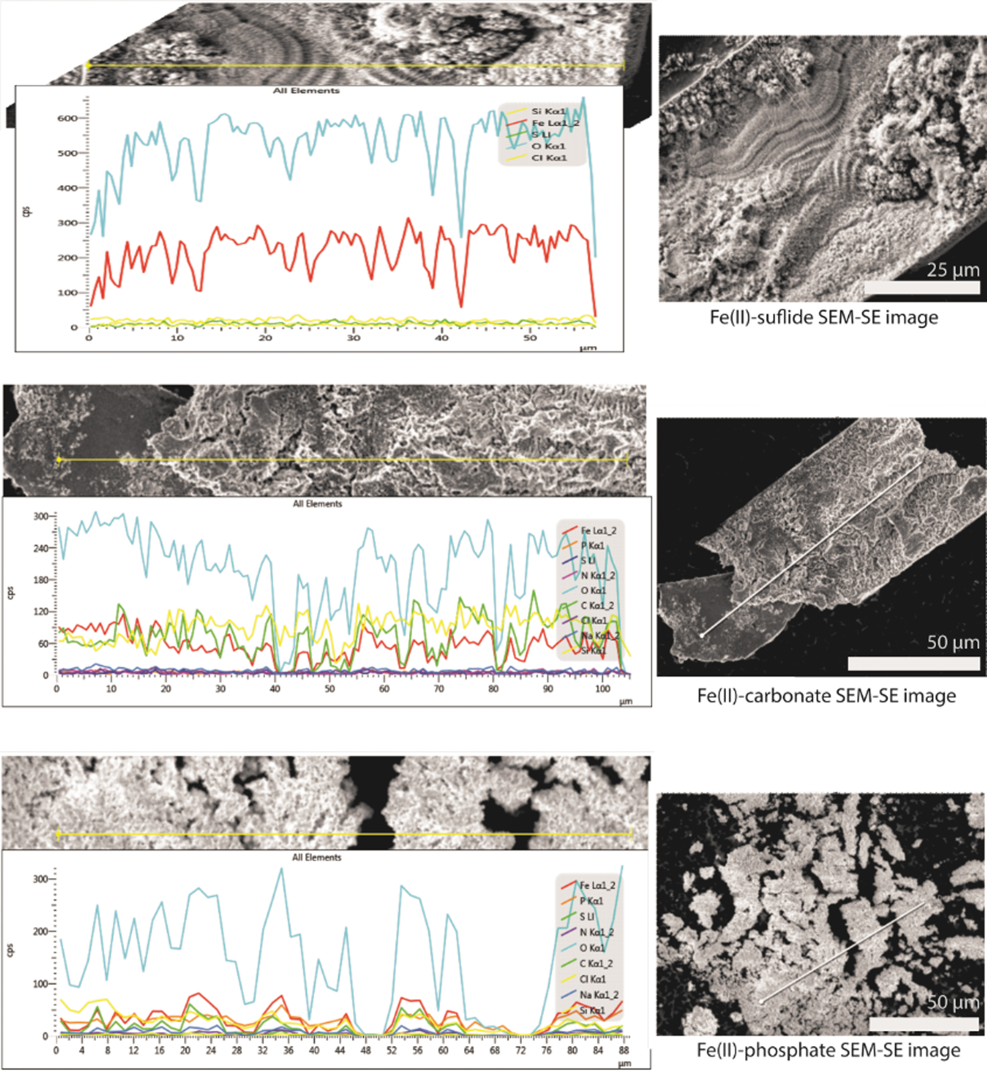
(Top) An example Fe(II)-sulfide “membrane.” Sulfur ratios are often very low, with Fe:O ratios of ∼1:2 or 1:2.5, consistent with FeO(OH) and Fe₂O₃. (Middle) An example EDS line scan of image from article Fig. 3. Fe:C:O ratio is ∼1:1:3, broadly consistent with FeCO₃. Material is often enriched in Fe to a ratio approaching 4:1:7, likely due to mixed iron oxide/iron carbonate species. (Bottom) An example EDS line scan. Fe:P:O ratio is ∼3:2:10, broadly consistent with Fe₃(PO₄)₂. EDS, energy-dispersive spectroscopy; SEM, scanning electron microscopy.

In summary, morphological and elemental results are broadly consistent with early, amorphous analogues to vivianite [Fe₃(PO₄)₂], siderite (FeCO₃), and iron sulfide within a variably concentrated matrix of iron oxides and iron oxyhydroxides. The anion-specific mineral analog production is validated by the direct instrumental evidence presented above, the anion-specific coloration (Fig. 2), morphology (Fig. 3), the precipitation rates (Supplementary Data, section 1.4), and the comparison of characteristic Raman spectra (Supplementary Data, section 1.5.3).

Diagenetic alteration of primary precipitates is common in natural settings, as water is driven from the coordinating matrix and exchange reactions occur (Stumm et al., 1983; Coleman, 1985). This diagenesis results in oxidation in the Fe(II)-phosphate and Fe(II)-sulfide material, with the Fe(II)-sulfide in particular losing the majority of its sulfur as evidenced by a loss of dark, black coloration within a day or so of formation.

The postdepositional processing and weathering of analogues are not considered in this work.

3.3. Flow and diffusion modeling

It is expected that the confined geometries of the microchannel will conspire with viscous fluid forces to prevent the inertial mixing of the Fe(II) and anion in these experiments, and that only diffusion will allow for reactant mixing to produce the material observed (Culbertson et al., 2002; Poonoosamy et al., 2019; Dutka et al., 2020). Diffusion is typically thought of as a “spreading” process where a localized concentration travels outward, becoming spread over a wider area but at lower concentration.

In the case of systems on the scale of the microchannel in this experiment, a constant supply of concentrated chemical species is provided by flow on one side of the channel coupled to that chemical's spreading diffusivity on the other side of the laminar flow boundary between solutions serves to form steep gradients at the interfacial boundary. The exact nature of those gradients is important for understanding the redox and pH environment under which the amorphous material will coordinate into a mineral analogue. We have shown elsewhere that these gradients and other forces within flowing systems are responsible for the accumulation of material at the channel's center in the first place (Pital et al., 2021).

To better understand the gradients produced by the interactions between diffusion and flow within the channel, a model was produced, which considers flow as the primary driver of diffusional extent and shape (details in Supplementary Data, section 1.2). As Fig. 7 demonstrates, the camera's eye view of experiments is an amalgamation of the precipitation profile over the entire depth of the channel. Diffusion across the interface between the two flowing reactant solutions is not homogeneous along the height of the channel, and inhomogeneities in earlier up-channel slices propagate down-channel to affect the precipitation boundary.

The prediction of concentration as shown in Fig. 5 is incomplete without an understanding of how that concentration translates into the drop in pixel albedo that are used to produce precipitate area curves such as those in Fig. 2. For this, an application of the Beer–Lambert Law is made to concentration profiles such as Fig. 8B.1. With the assumption that an absorbance of ∼0.1 (∼20% of incident light absorbed) is required for the albedo of a pixel to drop enough for that color change to be detectable, and the assumption that the amorphous iron sulfide has a molar extinction coefficient on the order of 10⁵ (Hong and Rabinowitz, 1970; Kawai et al., 2014), a total concentration of ∼140 μM is required across the entire channel height of a single pixel's area for the camera to detect a change.

FIG. 8.

(A) The 70 × 500 μm channel is viewed during experiments at approximately halfway down the length of the 15 mm channel. (A.1) An Fe(II)-sulfide experiment with precipitate forming at the channel centerline where reactant solutions meet. (B.1) Modeling of the diffusive overlap in reactive species is consistent with these observations, and (B.2) also allows for a micron-scale understanding of the chemical and fluid dynamic environment leading to the apparent precipitate area as viewed from above.

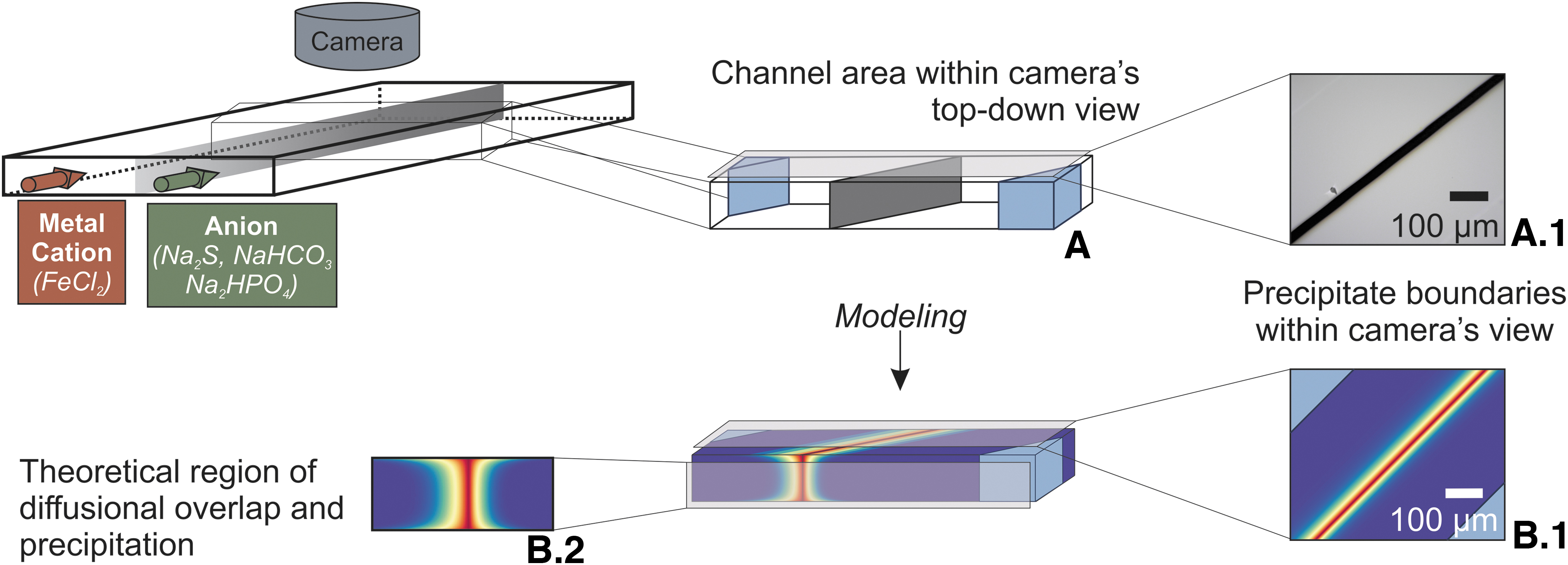
This value produces a modeled precipitation boundary that agrees well with observed experimental results for 100 μL/min as shown in Fig. 9. The above discussion is the lower bound limiting case for iron sulfide, given a known molar extinction coefficient and no contribution of light scattering. Explicit photon absorption is not required for light scattering by the accumulating colloidal precipitate that darkens pixel albedo, and the limiting assumption can therefore be roughly generalized to any coherent material that collects in a similar manner.

FIG. 9.

Modeled predictions of visible precipitation region due to diffusive overlap of Fe(II) and HS- are in good agreement with experimental results, a sampling of images of which is shown. Precipitate area under the simple model presented is expected to plateau at the blue model line (width is related to camera uncertainty), and actual results are broadly in line with this prediction.

It should be noted that flow rates <100 μL/min produce overestimations of precipitate boundaries because the model as presented does not take colloidal effects into account. Flow rates >100 μL/min, on the contrary, produce an underestimation of the actual precipitate boundary because the simple model here does not account for the viscous effects of colloids precipitating in an otherwise dilute solution. The discussion of these parameters is beyond the scope of this work and can be found elsewhere (Pital et al., 2021).

4. Discussion

The gradients predicted by the modeling above have profound implications for the accretion and fate of early, amorphous precipitate accretion. One example is the effect that the gradient of ionic strength has in influencing the equilibrium and instantaneous concentrations in a precipitation reaction. For a generic reaction $a \cdot A + b \cdot B c \cdot C$ , the instantaneous reaction quotient is given by $Q = \frac{{[C]}^{c}}{{[A]}^{a} {[B]}^{b}}$ by the law of mass action, with [species] representing the molarity of that species. In the generic case of an iron(II) precipitate, that instantaneous reaction quotient is shown in Eq. (1).

The reaction is in theory reversible; however, precipitation reactions depend on a solid having a low rate of dissolution. In either case, solid concentrations are not considered in reaction quotients or equilibrium calculations of this form, and so the precipitate contribution to mass balance goes to 1: $Q_{e i i e, o} = \frac{1}{[F e (I I)] \times {[A n i o n]}^{y}}; Q_{i t i,} = \frac{[F e (I I)] \times {[A n i o n]}^{y}}{1} .$ (1)

In the case where an equilibrium is reached, Q becomes the solubility product constant K _sp, and represents the equilibrium concentration of aqueous species in a considered chemical system in interface with a solid. This value is sensitive to many features of the chemical environment such as pH and ionic strength, which alter the electrostatic phase space reactants' experience when approaching each other along reaction coordinates. This feature of chemical systems is reflected in Eq. (2) with the consideration of a chemical activity (a).

Chemical activity is the product of the chemical activity coefficient (γ), a scalar multiplier that relates the activity of a chemical species in reaction to the actual molal concentration (moles_solute/mass_solvent as compared with the more familiar moles_solute/volume_solvent of molarity) in the reaction volume. Molal concentrations (m) are useful because volumes can change in the case of strong solvent effects or temperature changes. In many cases, the assumption of dilute effect is appropriate, and in the following discussion we assume m _{S e ies} ≅ [species] and substitute the more familiar molarity for molality: ${Q_{i t i}}_{, c t i v i t y} = {a^{x}}_{F e (I I)} \cdot {a^{y}}_{A n i o n} = {γ^{x}}_{F e (I I)} \cdot {γ^{y}}_{A n i o n} \cdot {m^{x}}_{F e (I I)} \cdot {m^{y}}_{A n i o n} .$ (2)

Equilibrium concentration of aqueous reactant ions will depend heavily on Eq. (2) (Ramos and McBride, 1996; Stefánsson, 2007; Sun et al., 2009). Consider the case where reactants exceed the balance of K _sp, such that precipitation is expected. In the application of Eq. (1), this is a straightforward accounting of chemical concentrations within the volume under consideration. If Eqs. (1) and (2) are set equal to each other and molality is assumed to be equivalent to molarity, it is clear that for situations where the combined activity coefficients deviate from ideality by even small amounts, large increases in the soluble molar concentrations accounting for activity ([species]) result to maintain the same K _sp. The lower the chemical activity of a chemical species is, the higher its concentration must be to approach the reactivity in ideal ([species]_s) conditions:

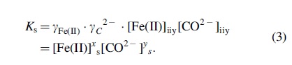
This mechanism is displayed above in an example of iron (II) carbonate [Eq. (3)]. Given a constant solubility of the solid, a solution of ∼1 mM FeCl₂ and 1 mM Na₂CO₃ ²⁻ will have a soluble ion concentration twice as high as expected due solely to chemical activity and ionic strength considerations. In other words, the decreased chemical activity at higher ionic strengths results in smaller masses of precipitate than would be expected strictly from concentration and solubility constants, resulting in larger actual concentrations of soluble ions that can exacerbate the diminishment of precipitation under experimental conditions.

This effect has a profound implication on the accretion and directing of precipitate colloids into the mass of the “membrane” (Pital et al., 2021). A full discussion of colloid dynamics is complicated and depends on surface charge and other considerations that are beyond the scope of this work; however, Fig. 10 shows that the general narrative of increased ionic strength shielding reactions and interactions that lead to mineral analog consolidation is consistent with the initial formation rates of precipitate for each of the chemical systems studied.

FIG. 10.

(Left) Model results predict a steep ionic strength gradient at the region of precipitation, and (Right) precipitate area over the initial accretion of precipitating material follows that trend. Increased ionic strength decreases the activity of Fe(II) and phosphate ions in particular due to their hydrated radii. Shaded regions represent 95% CI.

5. Conclusions and Future Directions

Precipitation of early, amorphous analogues of the minerals vivianite [Fe₂(PO₄)₃], siderite (FeCO₃), and iron sulfide has been produced in a microchannel, and analyzed by SEM, EDS, XPS, and Raman spectroscopy. In addition, the interplay between flow and diffusion within the channel and at the solution–solution interface where precipitation of these mineral analogues occurs has been modeled. Technique for measuring the precipitate area over time by automated analysis of timelapse images taken during the precipitation has been shown to be a useful tool in characterizing the chemical environment of the evolving system.

The questions of relevance in the astrobiology community often share a common thread of the interplay between organic matter and the geochemical context in which it is situated. The results presented here suggest a range of next steps in characterizing the interface between physical parameters such as flow and temperature, and chemical parameters such as pH, redox state, and concentration.

Do organics delivered from meteorites on early Earth survive in particular geochemical environments rather than globally, for example? This is clearly a complicated and involved question to address experimentally; however, an even more complicated question is the reverse: in an abiotic environment, how is the geochemical niche altered by the presence or absence of organics? What concentrations and combinations of organic species, if any, alter the natural range of geochemical complexities in systems with an aqueous interface layer? What complexity of conditions exists in purely abiotic geochemical systems? These are obviously complicated questions; however, any step toward addressing them must find its way through the kind of system presented here that allows for the gradients and forces endemic to the natural world.

Footnotes

Authors' Contributions

The article involves contributions of all authors. All authors have given approval to the final version of the article.

Author Disclosure Statement

No competing financial interests exist.

Funding Information

This work was performed in part at the Georgia Tech Institute for Electronics and Nanotechnology, a member of the National Nanotechnology Coordinated Infrastructure (NNCI), which is supported by the National Science Foundation (Grant ECCS-1542174). Work was supported with funding from the Blanchard Foundation, Georgia Institute of Technology, and the State of Georgia.

Supplementary Material

Supplementary Data

Abbreviations Used

Associate Editor: Christopher McKay

References

Ajmal

, Muhmood

, Usman

, et al. (2018) Phosphate removal from aqueous solution using iron oxides: adsorption, desorption and regeneration characteristics. J Colloid Interface Sci, 528:145–155.

Baaske

, Weinert

, Duhr

, et al. (2007) Extreme accumulation of nucleotides in simulated hydrothermal pore systems. Proc Natl Acad Sci U S A, 104:9346–9351.

Benhabib

, Chiesl

, Stockton

, et al. (2010) Multichannel capillary electrophoresis microdevice and instrumentation for in situ planetary analysis of organic molecules and biomarkers. Anal Chem, 82:2372–2379.

Bonfio

, Godino

, Corsini

, et al. (2018) Prebiotic iron–sulfur peptide catalysts generate a pH gradient across model membranes of late protocells. Nat Catal, 1:616–623.

Boucherit

, Hugot-Le Goff

, and Joiret

(1991) Raman studies of corrosion films grown on Fe and Fe-6Mo in pitting conditions. Corros Sci, 32:497–507.

Brown

, Viviano

, and Goudge

(2020) Olivine-carbonate mineralogy of the Jezero Crater Region. J Geophys Res Planets, 125:e2019JE006011.

Coleman

(1985) Geochemistry of diagenetic non-silicate minerals: kinetic considerations. Phil Trans R Soc London A Math Phys Sci, 315:39–56.

Culbertson

, Jacobson

, and Ramsey

(2002) Diffusion coefficient measurements in microfluidic devices. Talanta, 56:365–373.

Davranche

, Gélabert

, and Benedetti

(2020) Electron transfer drives metal cycling in the critical zone. Elements, 16:185–190.

10.

Dickson

(2019) Anaerobic intestine-on-a-chip system enables complex microbiota co-culture. Nat Rev Gastroenterol Hepatol, 16:390.

11.

De Faria

, Venâncio Silva

, and De Oliveira

(1997) Raman microspectroscopy of some iron oxides and oxyhydroxides. J Raman Spectrosc, 28:873–878.

12.

Dutka

, Starchenko

, Osselin

, et al. (2020) Time-dependent shapes of a dissolving mineral grain: comparisons of simulations with microfluidic experiments. Chem Geol, 540:119459.

13.

Genchev

and Erbe

(2016) Raman spectroscopy of mackinawite FeS in anodic iron sulfide corrosion products. J Electrochem Soc, 163:C333.

14.

Hanesch

(2009) Raman spectroscopy of iron oxides and (oxy) hydroxides at low laser power and possible applications in environmental magnetic studies. Geophys J Int, 177:941–948.

15.

Hazen

, Papineau

, Bleeker

, et al. (2008) Mineral evolution. Am Mineral, 93:1693–1720.

16.

Herbert Jr

, Benner

, Pratt

, et al. (1998) Surface chemistry and morphology of poorly crystalline iron sulfides precipitated in media containing sulfate-reducing bacteria. Chem Geol, 144:87–97.

17.

Heuer

and Stubbins

(1999) An XPS characterization of FeCO₃ films from CO2 corrosion. Corros Sci, 41:1231–1243.

18.

Hong

and Rabinowitz

(1970) Molar extinction coefficient and iron and sulfide content of clostridial ferredoxin. J Biol Chem, 245:4982–4987.

19.

Horgan

, Anderson

, Dromart

, et al. (2020) The mineral diversity of Jezero crater: evidence for possible lacustrine carbonates on Mars. Icarus, 339:113526.

20.

Jackson

(2016) Natural pH gradients in hydrothermal alkali vents were unlikely to have played a role in the origin of life. J Mol Evol, 83:1–11.

21.

Jin

, Li

, Algeo

, et al. (2016) A highly redox- heterogeneous ocean in South China during the early Cambrian (∼529–514 Ma): implications for biota-environment co-evolution. Earth Planet Sci Lett, 441:38–51.

22.

Kailer

, Nickel

, and Gogotsi

(1999) Raman microspectroscopy of nanocrystalline and amorphous phases in hardness indentations. J Raman Spectrosc, 30:939–946.

23.

Kawai

, Yamazaki

, Sobue

, et al. (2014) Electrochemical deposition of iron sulfide thin films and heterojunction diodes with zinc oxide. APL Mater, 2:032110.

24.

Keil

, Möller

, Kieß

, et al. (2017) Proton gradients and pH oscillations emerge from heat flow at the microscale. Nat Commun, 8:1–9.

25.

Kim

, Yee

, Nanda

, et al. (2013) Anoxic photochemical oxidation of siderite generates molecular hydrogen and iron oxides. Proc Natl Acad Sci U S A, 110:10073–10077.

26.

Kim

, Stockton

, Jensen

, et al. (2016) Pneumatically actuated microvalve circuits for programmable automation of chemical and biochemical analysis. Lab Chip, 16:812–819.Lane N (2017) Proton gradients at the origin of life. BioEssays 39:1600217.

27.

Lee

S-JJ

and Sundararajan

. (2010) Microfabrication for Microfluidics. Artech House, Norwood, MA, pp. 99–140.

28.

Legrand

, Sagon

, Lecomte

, et al. (2001) A Raman and infrared study of a new carbonate green rust obtained by electrochemical way. Corros Sci, 43:739–1749.

29.

Liu

and Kounaves

(2021) Degradation of amino acids on Mars by UV irradiation in the presence of chloride and oxychlorine salts. Astrobiology, 21(7):793–801.

30.

Masambi

, Dorfling

, and Bradshaw

(2016) Comparing iron phosphate and hematite precipitation processes for iron removal from chloride leach solutions. Miner Eng, 98:14–21.

31.

Matamoros-Veloza

, Cespedes

, Johnson

, et al. (2018) A highly reactive precursor in the iron sulfide system. Nat Commun, 9:1–7.

32.

Mielke

, Robinson

, White

, et al. (2011) Iron-sulfide-bearing chimneys as potential catalytic energy traps at life's emergence. Astrobiology, 11:933–950.

33.

Möller

, Kriegel

, Kieß

, et al. (2017) Steep pH gradients and directed colloid transport in a microfluidic alkaline hydrothermal pore. Angew Chem Int Ed, 56:2340–2344.

34.

Montague

. (1986) Influence of biota on erodibility of sediments. In Estuarine Cohesive Sediment Dynamics, edited by AJ

Mehta

. Springer, New. York, pp 251–269.

35.

Mullet

, Boursiquot

, Abdelmoula

, et al. (2002) Surface chemistry and structural properties of mackinawite prepared by reaction of sulfide ions with metallic iron. Geochim Cosmochim Acta, 66:829–836.

36.

National Research Council. (2019) The Limits of Organic Life in Planetary Systems. National Academies Press, Washington, DC.

37.

Perkins

and Garber

(2003) Raman spectroscopy of iron in aqueous carbonate solutions. J Solution Chem, 32:265–272.

38.

Pierri

, Tsamouras

, and Dalas

(2000) Ferric phosphate precipitation in aqueous media. J Crystal Growth, 213:93–98.

39.

Pital

, Kim

, and Stockton

(2021) Colloid precipitation and interactions at a flowing solution-solution interface in confined geometries. Colloids Surf A Physicochem Eng Asp, 629:127431.

40.

Poonoosamy

, Westerwalbesloh

, Deissmann

, et al. (2019) A microfluidic experiment and pore scale modelling diagnostics for assessing mineral precipitation and dissolution in confined spaces. Chem Geol, 528:119264.

41.

Ramos

and McBride

(1996) Goethite dispersibility in solutions of variable ionic strength and soluble organic matter content. Clays Clay Miner, 44:286–296.

42.

Stefánsson

(2007) Iron (III) hydrolysis and solubility at 25 C. Environ Sci Technol, 41:6117–6123.

43.

Stumm

, Furrer

, and Kunz

(1983) The role of surface coordination in precipitation and dissolution of mineral phases. Croat Chem Acta, 56:593–611.

44.

and Suarez

. (1997) In situ infrared speciation of adsorbed carbonate on aluminum and iron oxides. Clays Clay Miner, 45:814–825.

45.

Sun

, Nešić

, and Woollam

(2009) The effect of temperature and ionic strength on iron carbonate (FeCO₃) solubility limit. Corros Sci, 51:1273–1276.

46.

Tabata

, Sekine

, Kanzaki

, et al. (2021) An experimental study of photo-oxidation of Fe (II): implications for the formation of Fe (III)(hydro) oxides on early Mars and Earth. Geochim Cosmochim Acta, 299:35–51.

47.

Tan

and Sephton

(2020) Organic records of early life on Mars: The role of iron, burial, and kinetics on preservation. Astrobiology, 20:53–72.

48.

Wang

and Sherwood

(2002) Iron (III) phosphate (FePO4) by XPS. Surf Sci Spectra, 9:99–105.

49.

Weber

, Böttger

, Pavlov

, et al. (2015) Raman investigations of iron sulfides under various environmental conditions [abstract 1759]. In 46th Lunar and Planetary Science Conference Abstracts. Lunar and Planetary Institute, Houston.

50.

Zhang

, Algeo

, Cui

, et al. (2019) Global-ocean redox variations across the Smithian-Spathian boundary linked to concurrent climatic and biotic changes. Earth Sci Rev, 195:147–168.

51.

Zhang

and Brow

(2011) A Raman study of iron–phosphate crystalline compounds and glasses. J Am Ceram Soc, 94:3123–3130.

Supplementary Material

Please find the following supplemental material available below.

For Open Access articles published under a Creative Commons License, all supplemental material carries the same license as the article it is associated with.

For non-Open Access articles published, all supplemental material carries a non-exclusive license, and permission requests for re-use of supplemental material or any part of supplemental material shall be sent directly to the copyright owner as specified in the copyright notice associated with the article.

0.00 MB

8.46 MB