Water Vapor Adsorption Provides Daily,Sustainable Water to Soils of the Hyperarid Atacama Desert

Abstract

Water is necessary for all life on Earth. Water is so critical that organisms have developed strategies to survive in hyperarid environments. These regions with extremely low water availability are also unique analogs in which to study the physico-chemical conditions of extraterrestrial environments such as Mars. We have identified a daily, sustainable cycle of water vapor adsorption (WVA) and desorption that measurably affects soil water content (SWC) in the hyperarid region of the Atacama Desert in southern Perú. We pair field-based soil temperature and relative humidity soil profiles with laboratory simulations to provide evidence for a daily WVA cycle. Using our WVA model, we estimate that one adsorptive period—one night—increases SWC by 0.2–0.3 mg/g of soil (∼30 μm rainfall). We can plausibly rule out other water inputs during our field campaign that could account for this water input, and we provide evidence that this WVA cycle is driven by solar heating and maintained by atmospheric water vapor. The WVA may also serve to retain water from infrequent rain events in these soils. If the water provided by WVA in these soils is bioavailable, it could have significant implications for the microorganisms that are endemic to hyperarid environments.

1. Introduction

Water is necessary for all known life on Earth. However, life has developed strategies to survive all sorts of environments from freshwater lakes and tropical rainforests to hypersaline lakes and hyperarid deserts. In the search for life elsewhere, NASA has pursued a “follow the water” strategy to investigate the most probable targets for life contingent on the presence of liquid water. Our nearest neighbors in the solar system are dry, inhospitable places. However, scientists have been searching over the past several decades for life on these dry planets.

Mars is an extraordinarily dry planet, having lost virtually all its surface water ∼1 Ga through interaction with the solar wind (Terada et al., 2009; Kite, 2019). Water on modern Mars, though scarce, is almost entirely present as ice located in the polar caps and in the subsurface of higher latitudes (Piqueux et al., 2019). Smaller non-ice reservoirs of water include (1) atmospheric vapor (∼20–160 ppmv) (Savijärvi et al., 2015; Fedorova et al., 2021), (2) ephemeral deliquescent brines (Rennó et al., 2009; Toner and Catling, 2018), and (3) regolith adsorbed vapor (∼0.5–1.5 weight percent [wt %]) (Beck et al., 2010; Steele et al., 2017). Recent work has also incited a robust debate as to the presence of hypersaline lakes in the subsurface below the southern polar cap (Lauro et al., 2021; Smith et al., 2021).

Hyperarid environments (defined as an aridity index, the ratio of evapotranspiration to rain, of ≤0.05) (Bastin et al., 2017) are one of the best terrestrial analogs from which to understand the physical and chemical conditions on Mars and, eventually, arid exoplanets. The hyperarid, ecological region of the Atacama Desert, which spans Perú and Chile, is one of the driest environments on Earth and is a reasonably accessible place that mimics aspects of martian conditions (Houston and Hartley, 2003; Narvaez-Montoya et al., 2022).

Water inputs to the Atacama soils are rare and meager (∼2 mm/year) due to the rain shadow effect from the Andes (Houston and Hartley, 2003). Rain and fog events occur between ∼1 and 10 times per year on average, respectively (McKay et al., 2003; Valdivia-Silva et al., 2012). Despite the infrequency of rain and fog events, viable cells are found in the top tens of cm in these soils (Navarro-Gonzalez et al., 2003; Valdivia-Silva et al., 2011; Schulze-Makuch et al., 2018). Little is known about the relationship between water input and microbial activity or microbial growth in these environments, except that—counter intuitively—major inputs of water (e.g., during El Niño events) can negatively affect the microbial community by driving certain microbial species locally adapted to hyperarid conditions to extinction and favoring a select minority that is capable of tolerating osmotic-shock and hypersaline brines (Azua-Bustos et al., 2018).

Water Vapor Adsorption (WVA) is a phenomenon that increases soil water content (SWC) through van der Waals-type attraction between water molecules and soil particles (Fig. 1; see also Agam and Berliner, 2006). The WVA process occurs when the ambient atmospheric relative humidity (RH) is higher than the RH of the soil pore space (Agam and Berliner, 2006). Soil WVA has been studied extensively in agricultural settings, particularly in arid and semiarid environments (Kosmas et al., 1998; Kosmas et al., 2001; Agam and Berliner, 2004; Verhoef et al., 2006). It has been shown to provide biologically relevant amounts of water and induce microbial respiration in semiarid environments (McHugh et al., 2015).

FIG. 1.

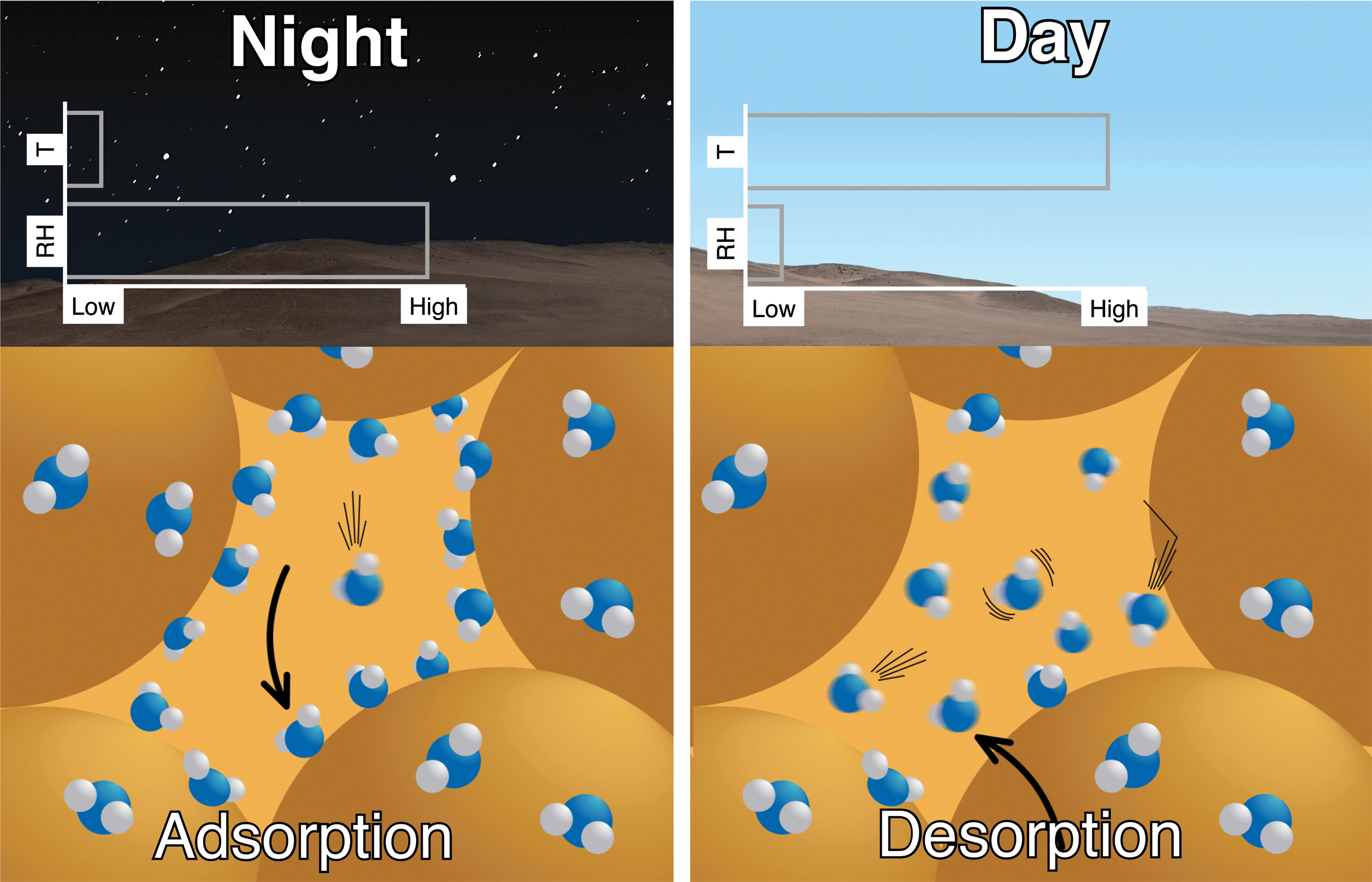
Conceptual diagram of WVA and desorption in response to environmental conditions in the Atacama Desert. Upper panels show representative surface temperature (T) and RH conditions during the night and day. Lower panels are a cartoon of water molecules (blue and white) in a soil matrix (dark tan spheres) with open pore space (light orange area in middle). Water molecules are either free in the pore space as [H₂O_(g)] (blurred) or adsorbed onto the soil surface (sharp). During the night (left panels), T is low, and most water molecules do not have enough energy to escape the surface adsorptive attraction (i.e., adsorbed water molecules). During the day (right panels), T is high, and most water molecules have sufficient energy to escape the surface attraction to enter the soil pore space (i.e., desorbed water molecules). RH, relative humidity; T, temperature; WVA, water vapor adsorption.

There are only a few direct measurements of WVA reported in hyperarid environments (Kaseke et al., 2012b; Kool et al., 2021); and, to our knowledge, no measurements have been made in the Atacama Desert. Here, we present field observations and laboratory simulation data along with an empirical model demonstrating the presence of an RH-driven WVA cycle in the hyperarid soils of the Atacama Desert. We developed a simple diffusion-advection-reaction model to interpret our field measurements; the model quantifies (1) the rates of WVA and desorption and (2) the effect of adsorption on SWC.

We compare the amount of water cycled by WVA with estimates of water input by rain and fog in this hyperarid region. We also compare our WVA estimates with those in other hyperarid environments. This work adds to our understanding of the total water budget of the near subsurface in hyperarid environments. It may also inform the search for microenvironments of water availability on Mars and, eventually, on dry exoplanets.

2. Materials and Methods

2.1. Field methods

2.1.1. Site

We performed field measurements and collected samples in a hyperarid region (aridity index ≤0.003) (Zomer et al., 2008) of the Atacama Desert in Southern Perú known as Pampas de la Joya, previously described by Valdivia-Silva et al. (2011). We characterized two sites, ∼1 km apart, located near ∼16.7°S, 72.1°W in a hilly desert landscape (Fig. 2A–D). The Mar de Quartz (MDQ) site is in a flat basin or playa (Fig. 2C). The Los Halitos (LH) site is located on a nearby hillside, roughly 5 m above the playa (Fig. 2D). Recent, nearby studies show relatively deep water tables of 50–150 m (Graber et al., 2021) and ∼200 m (Vera et al., 2021), indicating limited groundwater influence at the surface.

FIG. 2.

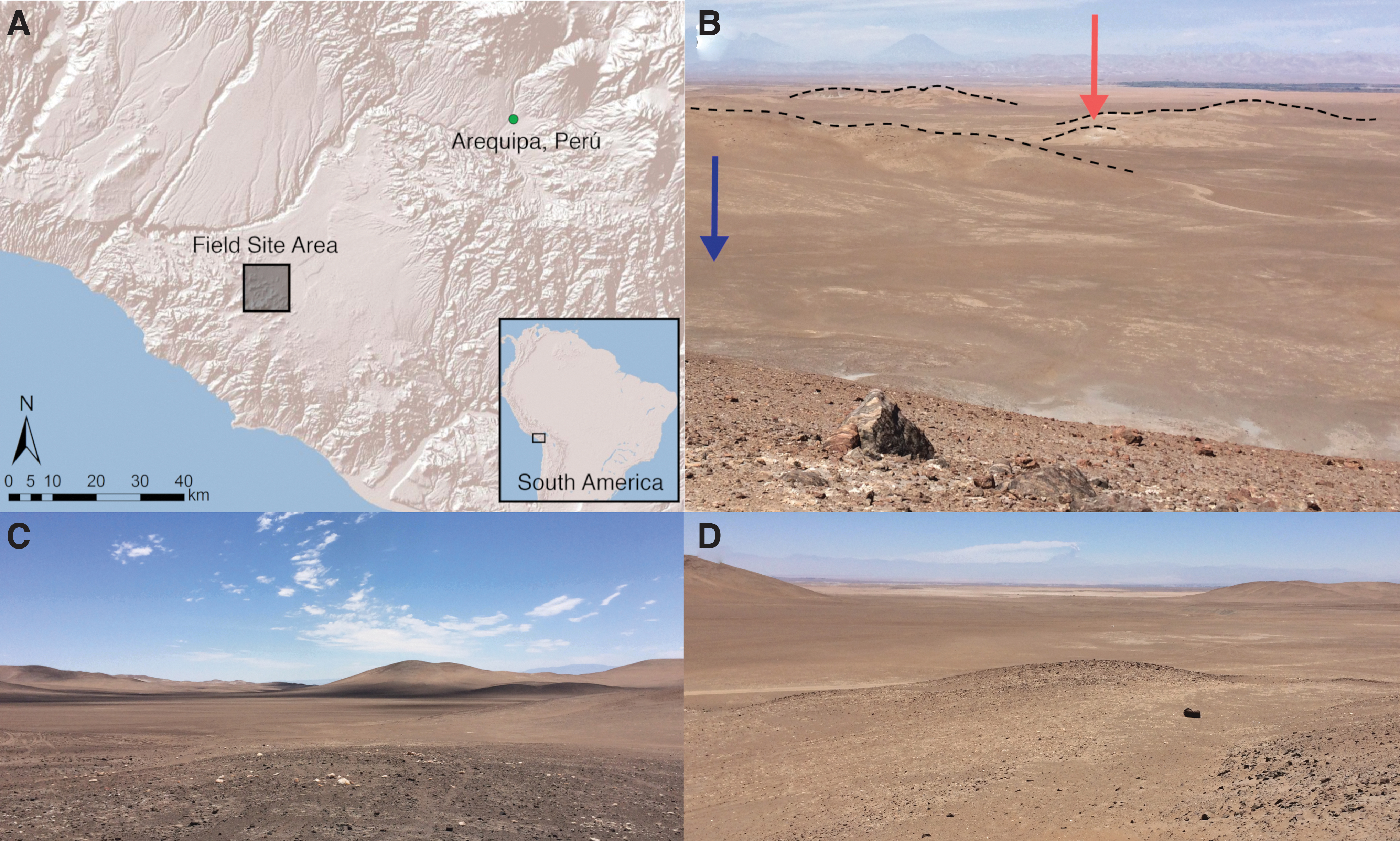
Map and photographs of the Pampas de la Joya field sites. (A) Overview map of the field area in southern Perú with the city of Arequipa noted for geographical context. (B) Overview photo of the field site showing MDQ (playa site; blue arrow) and LH (hillside site; red arrow) from a nearby hill facing ENE; note Misti volcano at center-left of the horizon. Black dashed lines emphasize the relief (∼10 m) in the landscape. (C) Photograph of the MDQ site facing NW. (D) Photograph of the LH site facing NNE. LH, Los Halitos; MDQ, Mar de Quartz. Photo credit: Donald Glaser.

2.1.2. Soil collection

We collected duplicate soil samples (∼2 m apart) at each site in October 2017. The top 5 cm (∼300 g) of surface soil was collected using a plastic hand spade and placed in a new, polyethylene zip-top bag. Samples were shipped back to the laboratory within 2 weeks and stored in the dark at 22°C before analysis and experimentation.

2.1.3. Soil temperature and RH

We measured soil temperature (T) and RH using a custom-designed and built sensor array. The sensor arrays were allowed to equilibrate in the soil for ∼36 h before data analysis (Supplementary Fig. S1). Collection of T and RH data occurred from October 1 to October 10, 2017, at MDQ, and from September 29 to October 4, 2017, at LH. The T and RH array was built from ½″ PVC tubing (1.5 cm internal diameter, 2.1 cm outer diameter) with six discrete chambers: one at each depth (i.e., 0, 2.5, 5, 10, 20, and 30 cm) to prevent air mixing between soil depths (Supplementary Fig. S2).

The PVC has a thermal conductivity similar to that of dry, sandy soil [e.g., 0.12–0.25 W/(m·K)] (Dashora et al, 2005; Robertson, 1988), so the sensors experience conditions similar to the adjacent soil. Two, 2 cm-diameter holes were placed 180° apart for air equilibration between the outer soil and the inside of the array chambers. Tyvek^® 1442R polyethylene membranes (Dupont^®, Wilmington, DE) were glued over the holes to prevent soil particles from entering the chambers while allowing air and water vapor to equilibrate across the membrane. A plastic polymer putty was used to separate the chambers due to its thermal insulation properties.

Temperature and RH were measured using Honeywell^® HIH7000 series capacitance sensors (Charlotte, NC). The data from the sensors were collected and stored using an Arduino^® pro-trinket microprocessor with an Adafruit™ microSD card breakout board. Coding and wiring schematics are available in a github repository (https://github.com/donnyglaser/Soil_TRH_SensorArray). Reported measurements at each depth were calculated as the mean of 10 readings (500 ms apart) every 20 min.

2.1.3.1. Sensor calibration and accuracy

The HIH sensors were calibrated before deployment. To calibrate temperature, the sensor was placed in an environmental chamber (Lab-Line^® model 850), allowed to stabilize for ≥30 min, and temperature recorded using a Fluke 52II meter with an LT-22N thermocouple probe. A 4-point calibration was performed with 10 sensor measurements at each temperature (i.e., 12.5°C, 17°C, 24°C, and 32°C) (Supplementary Fig. S3). The HIH sensor's temperature calibration had r ² = 0.99994; residuals for all calibration temperatures were <0.15°C (Supplementary Fig. S3).

To calibrate RH, the sensor was placed in a sealed glass chamber with a saturated salt solution buffer (Rockland, 1960). Humidity was allowed to stabilize for ≥24 h with each of 4 buffers [LiCl, 12% RH; Mg(NO₃)₂, 52% RH; NaCl, 75% RH; and H₂O, 100% RH] and 10 measurements were recorded (Supplementary Fig. S4). The HIH sensor's RH calibration had r ² = 0.99959; residuals for all calibration values of RH were <1.5% RH (Supplementary Fig. S4).

2.1.3.2. Sensor precision

We assessed the typical precision of the HIH sensor using data compiled from six depths, over ∼11 days at the MDQ site. We evaluated the standard deviation (SD) of repeated measures from the HIH sensor for temperature (binned over 10°) (Supplementary Table S3) and RH (binned over 20% RH) (Supplementary Table S4) to get a sense of the precision of the measurements. The average SD on the temperature reading was 0.008°C, and the maximum SD was 0.08°C; there is no relationship between temperature and SD, indicating that the sensors are equally precise across the entire range of observations.

The average SD for RH was 0.008% RH, and the maximum SD was 0.1% RH. There is a weak correlation between SD and RH, suggesting that values at high RH are somewhat less precise than measurements at low RH. However, the maximum observed SD (±0.1% RH) is similar to the manufacturer reported precision (±0.04% RH), indicating that the sensor is behaving nominally.

2.2. Laboratory methods

2.2.1. Soil characterization

Soil samples were sieved to 2 mm to remove gravel and cobbles and the <2 mm, fine-earth, fraction was used for characterization (Burt et al., 2014). We prioritized the fine-earth fraction because WVA is surface area-dependent (Leão and Tuller, 2014; Tuller and Or, 2005) and surface area decreases exponentially with increasing mean particle diameter (Allen, 2013). The soil particle size distribution was measured on a 40 g dry weight subsample using the hydrometer method (e.g., Day, 1965). Soil pH and conductivity were measured on a 1:2 (mass:mass) soil:deionized water (18.2 MΩ·cm water; Barnstead, Van Nuys, CA) slurry using an HACH HQ30d (Loveland, CO) multimeter with PHC201 and CDC401 probes, respectively. Extractable soil anions and cations were determined on filtered (0.2 μm, Supor^©; Pall, Port Washington, NY) subsamples of the 1:2 soil:deionized water mixture on Dionex DX600 (anions: Dionex IonPac AS11 analytical and IonPac AG11 guard columns) and DX120 (cations: Dionex IonPac CS12A analytical and IonPac SG11 guard columns) ion chromatographs, respectively according to methods from Shock et al. (2010).

A calibration curve from 0.1 to 10 ppm, periodic blanks (deionized water; one blank: five samples), and standards of known concentration were measured over the course of each sequence to ensure accurate ion concentration measurements. Bulk soil carbon and nitrogen content were determined in triplicate on dried, ground (i.e., 4 min in a ball-mill) soil samples. Briefly, soil subsamples treated with and without HCl fumigation (12 M, 8 h) were used to determine organic and total carbon content, respectively.

Milled, acidified/un-acidified soil was combusted using a Costech ECS 4010 (Valencia, CA) elemental analyzer with a thermal conductivity detector (Hedges and Stern, 1984). Inorganic carbon was determined as the difference between total carbon and organic carbon. Specific surface area was determined from Brunauer-Emmett-Teller (BET) isotherm analysis using N₂ adsorption in a Micromeritics^® Tristar II model 3020 (Norcross, GA) according to published methods (Bhambhani et al., 1972; Kaiser and Guggenberger, 2003); surface area samples were dried at 70°C under a gentle nitrogen stream to drive off excess water vapor before analysis.

Mineral abundances were determined by powder X-ray diffractometry (XRD) using a Bruker^® D8 (parameters: 5–65° 2θ, 0.02° steps, 2 s per step, Cu K-α radiation; Madison, WI) on soil samples ground to <20 μm using a McCrohn mill according to methods in Srodoń et al (2001). The resulting spectra were interpreted using “powdR,” an R library that calls the USGS's RockJock spectral database and optimizes fit by minimizing the weighted least squares residual error (Eberl, 2003; Butler and Hillier, 2021). Bulk soil porosity was calculated from helium pycnometry volume measurements on an AccuPyc 1330 (Micromeritics) using methods similar to Tamari (2004).

2.2.2. Simulation experiments

We performed laboratory incubations designed to simulate field conditions at a depth of 10 cm in the Atacama soils and measured the effect of changes in T at fixed RH on SWC (Supplementary Fig. S5). Temperature was controlled using a Lab-Line model 850 environmental chamber (Thermo Fisher, Waltham, MA). The chamber maintains T to within ±0.3°C and was used without a T ramp. Soil samples were placed into an air-tight polymethylmethacrylate enclosure (Mart^® Microbiology B.V., Lichenvoorde, NL) with a beaker containing ∼30 mL of a saturated LiCl solution to buffer at ∼12% RH (Supplementary Fig. S6) (Rockland, 1960). Before starting the experiment, the soil was dried at 50°C to a constant mass (i.e., stable to ±1.0 mg).

A lower drying temperature was chosen to eliminate all water (Section 2.2.3) without the risk of mineral dehydration (i.e., Strydom et al., 1995). Dry, <2 mm soil from each site (124 g for MDQ and 70 g for LH) in an 8-cm glass Petri dish was placed into the air-tight enclosure and the environmental chamber was cycled between 12°C (night conditions) and 35°C (day conditions) for 16 and 8 h intervals, respectively, to simulate the T changes observed in the field (Supplementary Fig. S5). The starting condition was 35°C; after 8 h, soil was removed from the enclosure and mass was determined on a Mettler Toledo model XS204 analytical balance (Columbus, OH).

The soil sample was then put back into the enclosure and cycled to the next T setting. Enclosure T and RH were measured using a one-sensor version of the field array setup described in Section 2.1.3. We modified the software to enable a higher data sampling rate and report the mean of 20 measurements (500 ms apart) every 5 min. The experiment was performed over a 4-day period. A control mass (75 g) consisting of a polyethylene Petri dish packed tightly with pyrite grains and sealed with electrical tape was incubated alongside the Atacama soils to assess the magnitude of changes in mass on a low surface area object of similar mass.

2.2.3. Soil water extraction and validation

Soil water was extracted from the experimental soils using a cryogenic trapping method similar to that presented by Koeniger et al (2011) (Supplementary Fig. S7). In brief, soil water was extracted after incubation for 48 h under night conditions (12°C, 12% RH). The soil (85 g) was placed into a 60 mL glass serum bottle (Wheaton^®, Rockwood, TN) connected to a 12 mL Exetainer^® (Labco, Lampeter, United Kingdom) with 1/16″ stainless-steel capillary tubing. The serum bottle was placed in a liquid nitrogen bath for ∼5 min; then, the headspace was removed using a vacuum pump to reduce the pressure ∼25 kPa, gauge (Supplementary Fig. S7A).

The serum bottle was removed from the liquid nitrogen and allowed to warm to room temperature for ∼15 min. To extract the water vapor adsorbed to the soils, the serum bottle was placed in a 90°C water bath and the connected Exetainer was immersed in an adjacent liquid nitrogen bath, facilitating transfer of water vapor from the soil into the Exetainer (Supplementary Fig. S7B). Over the course of 2 h ∼20 mg of clear liquid was transferred from the serum bottle to the Exetainer. The resulting extract in the Exetainer was analyzed using Fourier Transform Infrared Spectroscopy (FTIR) on a Bruker IFS 66v/S and compared with deionized water. A similar extraction of soil incubated at 50°C for 48 h failed to produce any measurable liquid; indicating that this soil was, in fact, dry.

3. Results

3.1. Field results

3.1.1. Soil temperature and RH

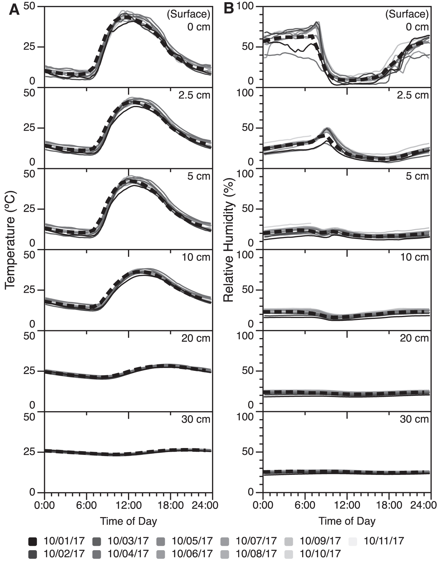
The surface T at MDQ (Fig. 3A) and LH (Fig. 4A) exhibits a strong diurnal pattern ranging from an average of ∼10°C at night to an average of ∼45°C during the day. The peak in surface T occurs between 11:50 and 13:35 (solar time). The sensors at depth show a similar diurnal pattern; however, the amplitude decreases with depth, and the timing of the peak in T is delayed by ∼5 h at the 20 cm depth. The 30 cm sensor shows a relatively stable T of ∼25°C.

FIG. 3.

Soil (A) temperature and (B) RH at the MDQ site as a function of time. Each panel shows multiple 24 h time series (thin lines) from a single depth arranged from 0 cm (surface) in the top panel down to 30 cm in the bottom panel. Thick black dashed line is an hourly average of all days. Each panel within (A, B) has the same y axis scale for direct comparison between panels. The gray-scale gradient distinguishes different days from the earliest date (black line, October 1) to the latest date (lightest gray, October 11). Both T and RH are relatively constant day to day, with the most variation observed in the surface RH.

FIG. 4.

Soil (A) temperature and (B) RH at the LH site as a function of time. Each panel shows multiple 24-h time series (thin lines) from a single depth arranged from 0 cm (surface) in the top panel down to 30 cm in the bottom panel. The thick black dashed line is an hourly average of all days. Each panel within (A, B) has the same y axis scale for direct comparison between panels. The gray-scale gradient distinguishes different days from the earliest date (black line, September 30) to the latest date (lightest gray, October 4). Both T and RH are relatively constant day to day, with the most variation observed in the surface RH.

The surface RH at MDQ (Fig. 3B) shows a strong diurnal pattern from ∼60% RH at night to ∼10% RH during the day. The shallowest sensor (2.5 cm) shows a daily pattern of ∼20% RH at night, a sharp peak of ∼40% RH around 09:00, and ∼10% RH during the day. The RH sensors at all greater depths (5–30 cm) show almost no diurnal pattern, and RH is roughly constant (±4% RH) over the entire day at ∼25% RH (Fig. 4B). The RH at LH (Fig. 4B) is comparable to MDQ; however, nighttime surface RH at LH (∼40% RH) is lower than during the same period at MDQ (∼60% RH).

The overall shapes and patterns in surface RH occur at both sites, but the magnitude and timing can vary. For example, the daytime RHs at both sites are similar at roughly 10% RH. There is a sharp, pronounced peak (∼70%) in RH at ∼07:30, just as T begins to increase. This same feature is evident at both sites, but is less pronounced, at MDQ. The 2.5 cm sensor at LH has an RH peak at 9:00 but the LH peak is smaller than the MDQ peak. The RH increases slowly from daytime values of 10% RH at ∼17:00 to nighttime values of 40–60% RH at 21:00.

3.2. Laboratory results

3.2.1. Soil characterization

Soil was analyzed in two fractions: bulk soil (all size fractions) and a <2 mm fraction. Bulk soil contains 17% gravel (>2 mm fraction) and 83% non-gravel (<2 mm fraction) at MDQ, and 13% gravel and 87% non-gravel at LH. In addition, LH had large (10–20 cm diameter) cobbles that were not sampled; the grain size difference between the two sites was noticeable by eye due to the presence of the large cobbles at LH. The texture of the <2 mm fraction at both sites is broadly a sandy loam (80% sand, 15% loam, and 5% clay) (Table 1).

Table 1.

Soil Texture and Chemistry Data for the Mar de Quartz and Los Halitos Sites

Parameter	Mar de Quartz	Los Halitos
Sand (%)	79.5 (±0.3)	84 (±0.1)
Silt (%)	16.8 (±1.55)	11 (±0.1)
Clay (%)	3.8 (±1.25)	5 (±0.0)
pH	6.46 (±0.190)	6.54 (±0.115)
Conductivity (mS/cm)	3.03 (±0.525)	6.29 (±0.220)
Total carbon (mg/g)	0.20 (±0.010)	0.16 (±0.025)
Inorganic carbon (mg/g)	0.04 (±0.005)	0.01 (±0.010)
Organic carbon (mg/g)	0.17 (±0.015)	0.15 (±0.010)
Total nitrogen (mg/g)	0.17 (±0.025)	0.34 (±0.000)
BET surface area (m²/g)	1.06 (±0.055)	0.473 (±0.0210)
Density (g/cm³)	1.38 (±0.001)	0.97 (±0.001)
Porosity (mL/mL)	0.516^a	0.655^a

Each value is the mean of measurements for two replicate samples, with one standard deviation in parentheses.

One measurement only.

BET = Brunauer-Emmett-Teller.

The MDQ soil has a slightly lower sand fraction and a higher silt fraction compared with LH. Both sites have similar, circumneutral pH (∼6.5) (Table 1). Soil conductivity at both sites is relatively high; with conductivity of ∼3 and ∼6 mS/cm, respectively (Table 1). Solid phase soil total carbon contents at both sites are similarly low at 0.2 mg/g (0.02 wt %); organic carbon was ∼80% of total carbon (e.g., 0.15 mg/g) (Table 1). Solid phase soil total nitrogen content is 0.17 mg/g (0.017 wt %) and 0.34 mg/g (0.034 wt %) at MDQ and LH, respectively (Table 1).

In general, replicate samples at the same site show high variability for most chemical analyses. The porosity of the MDQ soil was 0.52 and lower than that at LH, 0.66 (Table 1). The most abundant extractable major ions are Na⁺, Cl⁻, Ca²⁺, and SO₄ ²⁻, and concentrations are of the order of tens of mg/kg dry soil (Supplementary Table S1). Fitted MDQ and LH XRD spectra were created using the “powdR” R library with weighted least squares residual error of 0.12 and 0.07, respectively. Anhydrite is the most abundant mineral at MDQ, and actinolite is the dominant mineral at LH (Supplementary Fig. S8).

Both sites have roughly the same proportion of non-feldspar silicates (∼45%). The LH soil has the same proportion of feldspar and non-feldspar silicates (∼45%), whereas MDQ has relatively lower feldspar abundance (∼10%) (Supplementary Fig. S8). Evaporitic minerals were present at relatively higher proportions at MDQ (∼20%) than at LH (∼10%).

3.2.2. Simulated Atacama soil experiment

The results of the soil experiments are changes in soil mass as a function of T measured over the course of 80 h. Temperature ranged from 11°C to 13°C at night and from 32°C to 35°C during the day; RH was held at a fairly constant ∼12% RH (±2.7%) at all times (Supplementary Fig. S5). The large, sharp peaks in RH at 09:00 are due to the air-tight enclosure being opened and exposed to the ambient lab conditions for soil mass measurement; the peak decreases to target conditions within an hour.

Soil mass changes from the initial dry mass during the experiment were ∼180 mg (∼1.5 mg/g) for MDQ and ∼69 mg (∼1.0 mg/g) for LH. For soils from both locations, the first-time interval corresponded to a large positive change in mass, roughly 1 mg/g for MDQ and 0.5 mg/g for LH (Fig. 5). Starting from the second interval and continuing to the end of the experiment, soil mass increased during the nighttime (12°C) intervals and decreased during the daytime (35°C) intervals for soils from both sites. The control does not show the same magnitude of changes or the same pattern as the two soil samples. The control gains a total of ∼0.2 mg/g in mass over the experiment, an order of magnitude less than the soil samples.

FIG. 5.

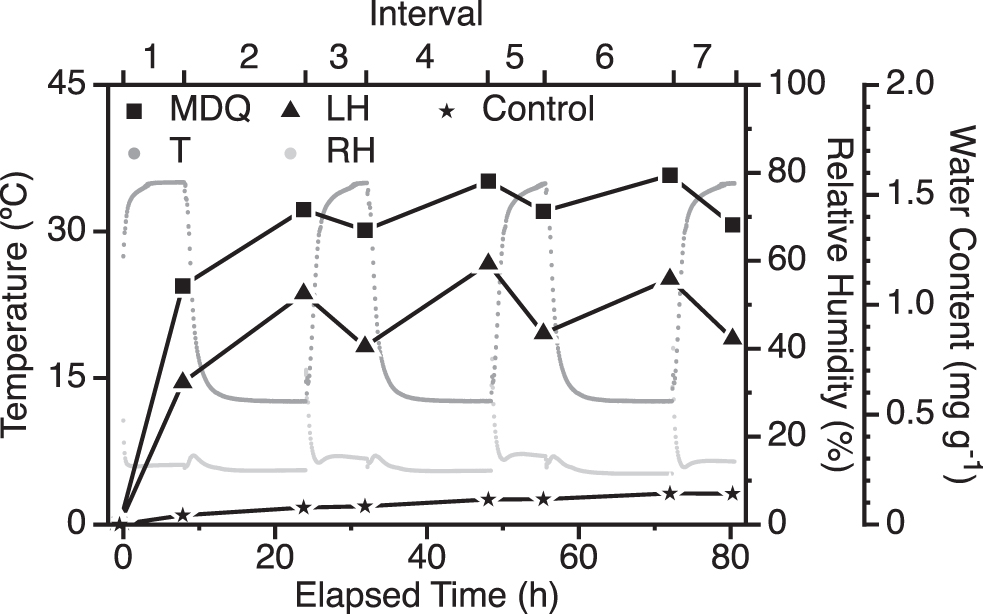
Change in mass during the simulation experiment as a function of time for soil samples from MDQ, LH, and a control. Left y axis (small, dark grey points) is enclosure temperature in °C. First right y axis (small, light grey points) is enclosure RH in %. Right most y axis is sample soil water content for MDQ (black squares), LH (black triangles), and control (black stars). Water content was calculated by comparing sample mass with dry mass. Samples were incubated for 82 h, and T changed from 12°C to 35°C on a 16:8 h cycle to simulate night/day conditions. RH was buffered at ∼12% RH. Sharp deviations in RH at the beginning of each interval are due to opening of the enclosure to measure the samples. The upper x axis ticks show points when the chamber temperature was changed to create the simulated night and day intervals. We observe increases in water content after intervals of cool conditions (12°C; nighttime) and decreases in water content after intervals of hot conditions (35°C; daytime). The control gains a small amount of water over the experiment, but at a much smaller magnitude compared with the soil samples; the control does not show decreases in water content during the hot intervals.

3.2.3. Soil water extraction and validation

Cryogenic extraction of 85 g soil yielded 22.6 mg of a clear liquid. The liquid exhibited FTIR absorption features at 1650 and 3370 cm⁻¹ that were similar to the peaks present in a deionized water standard (Supplementary Fig. S9). Results of a residual analysis show little difference (≤0.005 AU [absorbance units]) between the peaks for the liquid extracted from the soil and a water standard in the two regions of interest (Supplementary Fig. S9B).

4. Discussion

Here, we develop a diffusion-advection-reaction model to interpret the soil absolute humidity profiles as a two-part linear approximation from which we calculate water vapor flux via diffusion, and a reaction term that we interpret as WVA.

4.1. Subsurface temperature, RH, and absolute humidity in the pore space

Absolute humidity ([H₂O_(g)]), as compared with RH, is the concentration of water per unit volume and is not commonly measured directly. Absolute humidity is calculated using modeled saturation partial pressure of water that is an exponential function of T. The RH sensor measurements are calibrated in units of pressure, and it is necessary to convert to water concentration. We calculate [H₂O_(g)] using an entropy maximization framework developed by Koutsoyiannis (2012) based on RH, assuming ideal gas conditions. We observe that RH from 5 to 30 cm depth is relatively stable (±4% RH) over a diurnal cycle whereas T varies from ∼10°C to 45°C at the 5 cm depth. Considering this, and the fact that [H₂O_(g)] is a function of both T and RH, we infer that [H₂O_(g)] must be driven almost entirely by T in the subsurface, where our measured RH is nearly constant.

Figure 6A shows [H₂O_(g)] as a function of T for both sites at 5 cm depth. This indicates that there is a moderately strong positive correlation between T and [H₂O_(g)] that follows contours of fixed RH. Conversely, Fig. 6B shows [H₂O_(g)] as a function of RH, and there is little to no correlation as the data array vertically with RH. This suggests that the effect of RH on [H₂O_(g)] in these soils is negligible.

FIG. 6.

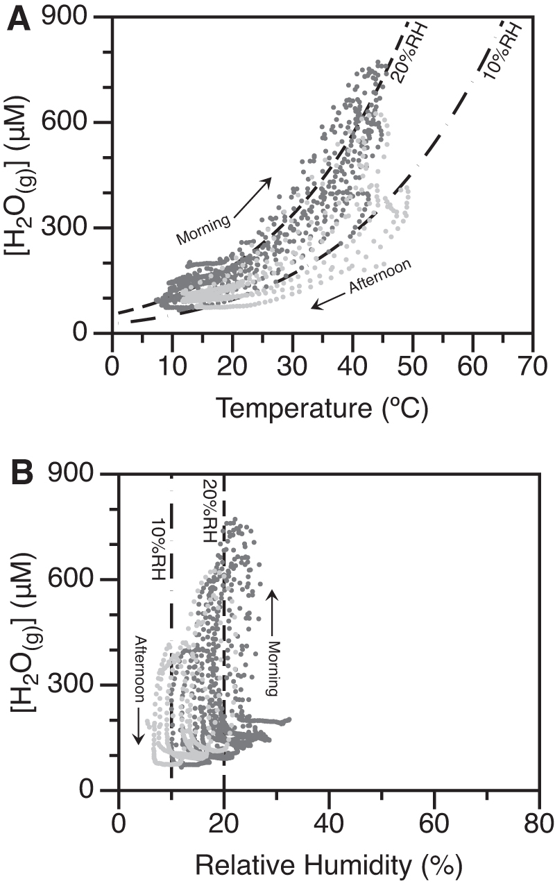
Absolute humidity ([H₂O_(g)]) for all days at 5 cm depth in the soil pore space as a function of (A) temperature and (B) RH at MDQ (dark grey) and LH (light grey). Black dashed lines are contours of constant RH at 10% (long dash) and 20% (short dash). The RH contours in (A) are calculated using the entropy maximization framework described in Section 4.1 (i.e., Koutsoyiannis, 2012). There is a moderately strong positive correlation between [H₂O_(g)] and T that follows the RH contours (A). Hysteresis in the curves is evident as a function of time such that [H₂O_(g)] increases over the course of the mornings and decreases in the afternoons in a clockwise loop (noted by arrows). There is no relationship between [H₂O_(g)] and RH as the data align almost vertically (B); counterclockwise hysteresis over the day is noted. These data suggest that diurnal changes in the subsurface can be driven primarily by changes in temperature, as heat is conducted through the soil column and RH is nearly constant.

The stability of RH over the course of the day at 5 cm depth (and down to 20 cm due to the diurnal T fluctuations) suggests the presence of some process that maintains roughly constant RH. It is plausible that deliquescent salts may buffer the RH of the pore space. In order for salts to buffer at the low RH values observed (∼20% in MDQ and ∼10% in LH), they must have a low deliquescent relative humidity (DRH); examples include LiCl, certain other chlorides, chlorates, or perchlorates.

We were unable to detect the presence of any salts with low DRH, based on X-ray diffraction. However, they could be present at abundances <3 wt %. Recent work has shown the colligative effects of salt mixtures on deliquescence, with the effect of reducing DRH relative to pure minerals (Dupas-Langlet et al., 2013; Gough et al., 2014; Toner and Catling, 2018). So, mixtures of salts could potentially buffer the RH we observe at MDQ and LH. However, common-ion effects can increase DRH and counteract the colligative effects of salt mixtures (Allan et al., 2016). Thus, RH control by deliquescence will depend on the specific salts present; however, it is plausible that low abundance salts could be present, buffering the subsurface RH.

Our ion chromatography results for soil extracts (Supplementary Tables S1 and S2) may be consistent with salt-buffered RH in the soils. The LH site has lower RH at 5 cm depth (∼10%) and a higher salt concentration (6.29 mS/cm) compared with the MDQ site (∼20%; 3.03 mS/cm). In addition, LH has a higher abundance of Cl⁻ (57.0 mg/kg) compared with MDQ (7.1 mg/kg). Further work would be required to positively identify salts present at trace levels in these soils.

It is also plausible that the WVA process itself maintains the constant RH at depth. In this case, the soil particle surfaces may act as a source and sink for water vapor, which has the effect of maintaining stable RH in the pore space.

Surface T peaks between 11:50 and 13:35 (solar time), which is ∼45 min earlier than previous similar observations of surface temperature in the Atacama (McKay et al., 2003). Another point to note in our observations of soil T is the delay in timing of the peak T at 20 cm relative to the peak T at the surface. Modeled soil temperatures as a function of depth and time (Gao et al., 2010; see their equation 4c) predict that T at 20 cm should peak ∼6 h after the peak surface T; our observations show a delay of ∼5 h. These observations may be the result of non-conductive heat sources; for example, the lack of water in these soils leads to reduced latent heat. More research is needed to investigate the energy balance of these soils and its effect on water inputs.

4.2. WVA model

A 1-D mass transport, diffusion-advection-reaction, model (WVA model) was developed to interpret the field data and is available in its entirety in a github repository (https://github.com/donnyglaser/SoilProfile_DiffusionReaction_Model). Using the field-collected soil T and RH profiles as input parameters (described in Section 2.1.3), we calculate WVA: $\frac{\partial [H_{2} O_{(g)}]}{\partial t} = D i f f + A d v + R x n,$ (1)

where [H₂O_(g)] is water vapor concentration, t is time, Diff is diffusive transport, Adv is advective transport, and Rxn is the reaction term. Each term in Eq. 1 has units of μmol/(cm³·s), that is, a change in [H₂O_(g)] per time. We assume that advective transport though the soil is negligible and that [H₂O_(g)] is in pseudo steady state on timescales of tens of minutes or more; therefore, we can simplify Eq. 1 as: $0 = D i f f + R x n,$ (2)

and balance the diffusive component against the reaction component. We use Fick's second law of diffusion to define diffusive transport: $D i f f = D \frac{\partial^{2} [H_{2} O_{(g)}]}{\partial z^{2}} = \frac{d J}{d z},$ (3)

where D is the diffusion coefficient in units of m²/s, $\frac{\partial^{2} [H_{2} O_{(g)}]}{\partial z^{2}}$ is the second derivative of [H₂O_(g)] with respect to depth (z), and J is the water vapor diffusive flux.

4.2.1. Water vapor diffusive flux

A gradient of [H₂O_(g)] with respect to depth will drive diffusive transport of water vapor from high concentration to low concentration. Here, we use Fick's first law of diffusion to solve for the water vapor flux (J): $J = - D \times \frac{\partial [H_{2} O_{(g)}]}{\partial z} .$ (4)

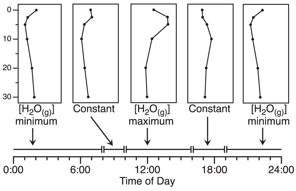
To solve this equation, we calculate $\frac{\partial [H_{2} O_{(g)}]}{\partial z}$ , in units of μM/cm (μmol/cm⁴), using a linear regression to approximate the [H₂O_(g)] versus depth profiles described in Section 4.2.2. Most of the [H₂O_(g)] versus depth profiles exhibit a two-part nature due to the presence of an [H₂O_(g)] minimum or maximum (Fig. 7). We consider the flux of the upper (J_up ) and lower (J_lo ) portions of the profile separately and then calculate the change in J (dJ; Eq. 5) to obtain the reaction term (Rxn), which we interpret as WVA (Eq. 6); that is:

FIG. 7.

Representative [H₂O_(g)] profiles and their approximate time periods over the course of a day. Vertical axis (in cm) and horizontal axis (in μM) are the same for all five panels.

d J = - J_{u p} + J_{l o}, a n d

(5)

W V A = - R x n = \frac{d J}{d z},

(6)

where dz is the combined depth of the upper and lower portions of the profile (Supplementary Fig. S10). Here, we use the convention that positive WVA is adsorption ([H₂O_(g)] minimum) and negative WVA is desorption ([H₂O_(g)] maximum). Overall, the WVA model allows us to calculate the WVA rate and allows the estimation of changes in SWC.

4.2.2. Profile identification and simplification

All [H₂O_(g)] profiles were classified as either (1) [H₂O_(g)] minimum, (2) [H₂O_(g)] maximum, or (3) constant (Fig. 7). The details of this classification scheme are described in Section S.1 in the Supplementary Data. Each [H₂O_(g)] minimum and [H₂O_(g)] maximum-type profile was simplified into upper and lower spatial regions that can be approximated by linear regression. This is because the upper and lower regions have slopes of an opposite sign and must be linearized separately to calculate dJ and thus, WVA.

4.2.3. Diffusion coefficient

The diffusion coefficient, D, is a function of porosity and T, which we calculate (in units of cm²/s), according to: $D = 0.073 {[\frac{(S - 0.1)}{0.9}]}^{2} {[\frac{T}{273}]}^{1.75},$ (7)

where S is bulk soil porosity and T is temperature in kelvin (e.g., Jabro, 2009; Troeh et al, 1982). To calculate S, in units of cm³/cm³ we use: $S = \frac{V_{p}}{V_{t}};$ (8)

where V_p is the pore volume and V_t is the total volume of the soil. We assume constant porosity as a function of depth for each site (Table 1). We calculate separate diffusion coefficients for the upper and lower profiles (D_up and D_lo ) because T differs significantly in the two regions of the profile at different times of the day (Supplementary Fig. S10 and Supplementary Figs. S16–S20). Temperature is calculated by interpolating the two nearest data points between the surface and the reaction point (T_up ) and between the reaction point and the reaction bottom (T_lo ) (Supplementary Fig. S10). The average upper and lower T (T_up and T_lo ) calculated is equal to T in Eq. 7 and is used to solve for the upper and lower diffusion coefficient (D_up and D_lo ), respectively.

4.2.4. WVA model output

The output of the WVA model generates values of WVA rate [μmol/(cm³·s)] that we present over time (Fig. 8). Values are positive during periods of WVA (i.e., [H₂O_(g)] minimum) and negative during periods of water vapor desorption (i.e., [H₂O_(g)] maximum). Trends in WVA rate are similar for both sites. The WVA rate begins positive at ∼0.0002 μmol/(cm³·s) from midnight until ∼7:00. From ∼7:00 to ∼9:00, there is a marked increase in WVA rate to ∼0.0003 observed on most days. Negative WVA values reach a minimum between −0.0007 and −0.0015 μmol/(cm³·s) between 11:00 and 12:00, after which there is a gradual trend toward more positive values of WVA rate. The WVA rates switch back to positive values of ∼0.0003 μmol/(cm³·s) at ∼17:00, gradually decreasing to ∼0.0002 μmol/(cm³·s) at midnight.

FIG. 8.

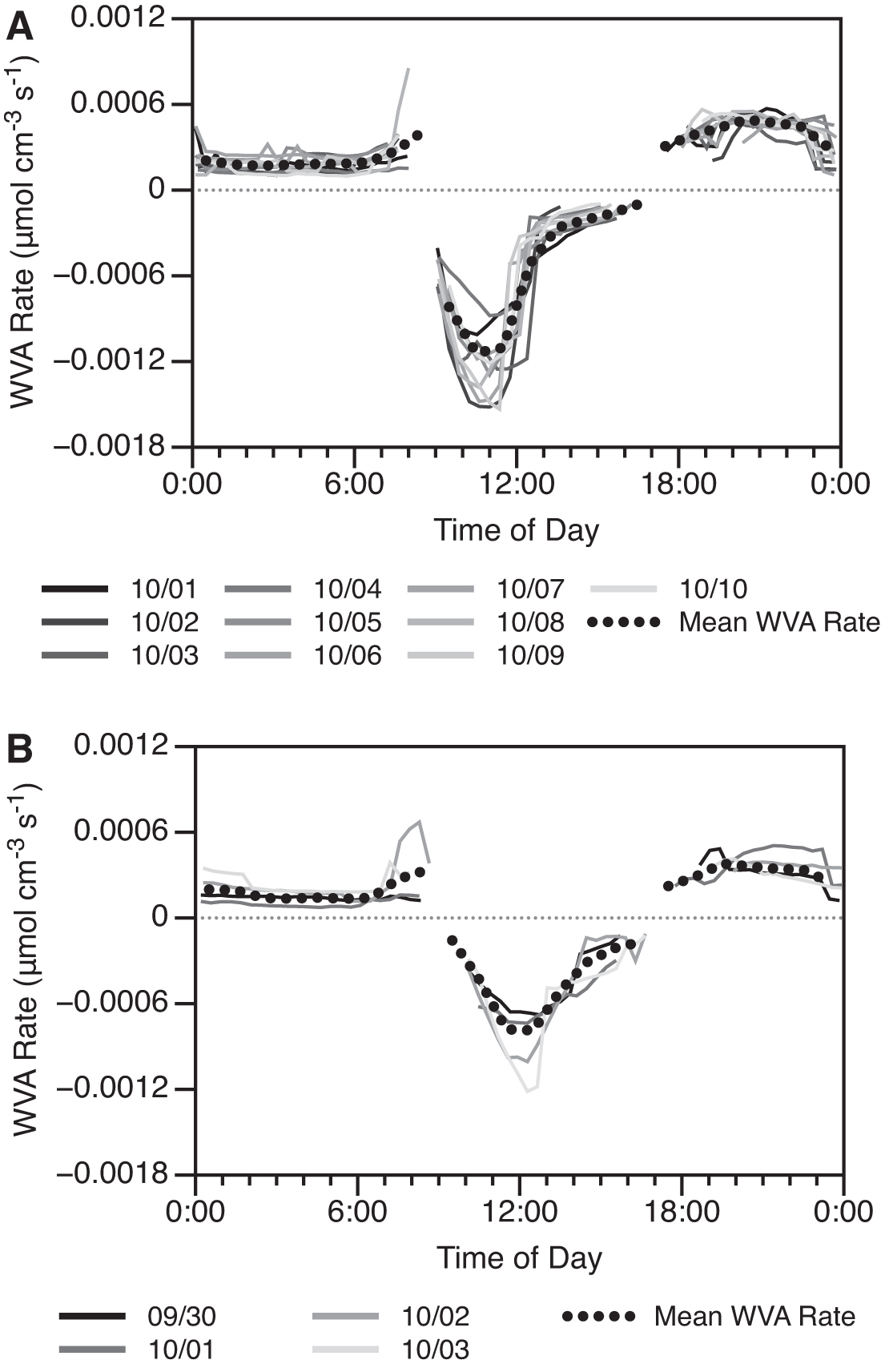
Results of WVA model showing WVA rate over time at (A) MDQ from October 1 (black) to October 10 (light grey) and (B) LH from September 30 (black) to October 3 (light grey). Thick black dotted line shows the hourly mean WVA rate for all days. Positive WVA rate indicates periods where water vapor is removed from the soil pore space (adsorption). Both sites show similar patterns of WVA rate with time. (A) Shows steady adsorption [∼0.0002 μmol/(cm³·s)] from midnight to 7:00, with a slight increase in adsorption [∼0.0004 μmol/(cm³·s)] at ∼8:00. At ∼9:00, WVA rate switches from positive to negative (desorption) and sharply decreases from approximately −0.0008 to approximately −0.0012 μmol/(cm³·s) at ∼11:00. The WVA rate increases until ∼17:00 when the WVA rate switches from negative back to positive at ∼0.0004 μmol/(cm³·s) slowly decreasing to ∼0.0002 μmol/(cm³·s) at midnight. (B) (LH) shows a similar pattern as (A) (MDQ); however, there are much less data from which to make definitive interpretations. This shows a daily cycle of WVA and desorption.

We integrated WVA rate [μmol/(cm³·s)] over time to produce a change in WVA over a specific time interval (μmol/cm³). We then summed all the changes in WVA over the course of a day to produce cumulative WVA, representing the net adsorption or desorption of water in the soils (Fig. 9). Positive cumulative WVA indicates net adsorption. Over the duration of observation at MDQ (10 days), we calculate a slightly negative cumulative WVA of −4.4 μmol/cm³, indicating a minimal loss of water over this period. At LH, we calculate a slightly negative cumulative WVA of −3.5 μmol/cm³, indicating a similarly negligible water loss over the observation period (4 days). Our observational period is too short to make overall generalizations of long-term WVA.

FIG. 9.

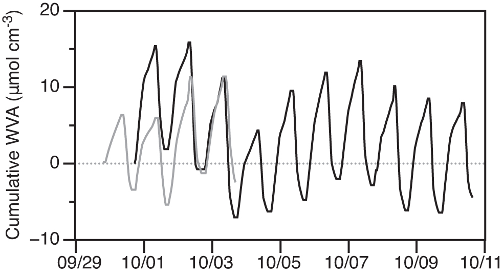
Cumulative WVA, that is, total water added/removed from the soil column per unit area, at MDQ (black) and LH (grey). Positive cumulative WVA indicates net adsorption (increased soil water content), and negative cumulative WVA indicates net desorption (decreased soil water content). Cumulative WVA at MDQ and LH indicate minimal water loss (3.5–4.4 μmol/cm³) over the study period.

4.2.5. Soil water content

Changes in SWC, the amount of H₂O associated with the soil particles (mg/g¹), can be estimated from WVA (μmol/cm³) by dividing by soil density (g/cm³). This method cannot determine absolute SWC but can assess relative changes in SWC over the adsorption or desorption periods. At MDQ, we calculate average changes in SWC of 0.19 and −0.17 mg/g for the adsorption and desorption periods, respectively (Table 2). Similarly, we calculate average changes in SWC of 0.20 and −0.22 mg/g at LH for the adsorption and desorption periods, respectively (Table 2).

Table 2.

Change in Soil Water Content at Both Sites Based on Field Data and Lab Simulation Results

Site	Observation	Change in soil water content (mg/g)
Site	Observation	Adsorption		Desorption
Mar de Quartz	Field data^a	0.19	(±0.02)	−0.17	(±0.03)
Mar de Quartz	Lab simulation^b	0.25	(±0.08)	−0.15	(±0.05)
Los Halitos	Field data^c	0.20	(±0.07)	−0.22	(±0.03)
	Lab simulation^b	0.34	(±0.07)	−0.28	(±0.03)

Values are the mean of all observations ±1 standard deviation.

n = 10; ^b n = 3; ^c n = 4.

These changes in SWC are in very good agreement with the changes in SWC observed independently in the simulation experiment (Section 4.3.2) (Table 2). The similar magnitudes of adsorption and desorption indicate that SWC is in rough steady state over the course of several days with no appreciable net loss of water from the soil (or gain to the soil). These changes in SWC are localized to the upper and lower profile regions of the soil, typically the top 10–20 cm (Supplementary Fig. S10). An increase in SWC of 0.20 mg/g over the top 10 cm of soil would equate to 20–30 μm of rain equivalent per day from WVA.

4.3. Laboratory simulations of WVA

4.3.1. Soil characteristics

The SWC changes in response to changes in T in our laboratory simulations (Fig. 5) indicate that MDQ soils have higher steady state (they reach a higher asymptotic plateau) water retention compared with LH soils (i.e., 1.5 and 1.0 mg/g soil, respectively). This is most likely due to the higher BET surface area of MDQ soils (∼1.05 m²/g soil) compared with LH soils (∼0.47 m²/g soil) (Table 1). Organic carbon is a highly adsorptive species that is capable of adsorbing ≥300 times the water observed in this experiment (Liu et al., 2017).

However, both samples in this experiment have very low organic carbon content (∼0.16 mg/g; ∼0.016 wt %), discrediting the idea that organic carbon content could be driving either (1) the overall WVA process, or (2) the differences in steady state water retention between MDQ and LH. The difference in steady state water retention could also be due to the significant differences in mineralogy for the two sites. (Supplementary Fig. S8). For example, the high evaporite content at MDQ could enhance WVA (or perhaps deliquescence); alternatively, the high feldspar content at LH could contribute to reduced WVA. We know of no published work that specifically explores the role of mineralogy in WVA.

4.3.2. Changes in SWC

The results of the laboratory simulation show a reasonably regular oscillation in mass after an initial equilibration time (∼24 h) for both MDQ and LH soils (Supplementary Fig. S11). We interpret this as evidence that the experiment reached a state where the increases and decreases in mass were roughly the same for cold and hot periods, respectively. In other words, WVA/desorption adds and removes roughly equal amounts of water into and out of the soil in our experiment (Table 2).

The increase in mass is most parsimoniously interpreted as adsorption of water to the soil grains when T is low. Similarly, mass decreases when T is increased, and water is desorbed into the vapor phase. Our experiments generated an average increase (trough-to-peak) in SWC of 0.25 ± 0.06 mg/g for MDQ and 0.34 ± 0.16 mg/g for LH (Table 2). All SWC increases for both samples are significantly different from zero. These results are in quite reasonable agreement with our WVA model-derived estimates of SWC increase of 0.19 and 0.20 mg/g for MDQ and LH, respectively (Table 2). The excellent agreement in SWC between the field and lab results suggests that our field observations are evidence for measurable WVA.

4.4. Evidence for WVA in hyperarid soils

We have provided several lines of in situ and laboratory evidence to support a daily WVA and desorption cycle in the soils of one of Earth's driest environments, the Atacama Desert.

4.4.1. WVA modeling

The output of the WVA model (Fig. 8) shows periods of positive WVA rate (i.e., between ∼17:00 and ∼9:00) at both field sites. In addition, our WVA model shows periods of negative WVA between ∼9:00 and ∼17:00 at both sites. We assert that a positive WVA rate is a measure of water vapor moving from the pore space and adsorbing to soil particles, thus increasing SWC (Fig. 1). Conversely, a negative WVA rate corresponds to water desorbing from soil particles and moving into the pore space, thus decreasing SWC (Fig. 1).

Supplementary Figure S12A shows an [H₂O_(g)] minimum-type profile with the directionality of diffusive water vapor transport indicated. At 5 cm depth, [H₂O_(g)] should increase over time, as water vapor is supplied from the top and bottom. This would result in a relatively straight [H₂O_(g)] profile if diffusion were the only process acting in these soils. However, this is not what we observe; the [H₂O_(g)] minimum-type profile is stable over 12–16 h. This indicates that a reaction, or some other physical process is removing water vapor from the pore space to maintain the [H₂O_(g)] minimum in the profile. Supplementary Figure S12B shows a [H₂O_(g)] maximum-type profile with the direction of diffusive water vapor transport shown.

Like the [H₂O_(g)] minimum-type profiles, the [H₂O_(g)] should change over time if diffusion were the only process acting on pore space water vapor. We observe [H₂O_(g)] maximum-type profiles that are stable for 4–5 h, indicating a reaction process that is adding water vapor to the pore space during this time.

4.4.2. Laboratory experiments

The results of an 80-h simulation experiment show both increases and decreases in SWC inversely related to increases and decreases in T (Fig. 5). These results are consistent in directionality and magnitude with the modeled field results. In both cases, we observe increased SWC during nighttime (12°C) conditions and decreased SWC during daytime (35°C) conditions. Cryogenic extraction of a liquid with FTIR characteristics similar to those of water from the simulation soils provides strong evidence that the cause of increased mass during the nighttime conditions is water (Supplementary Fig. S9).

4.4.3. Differences between surface and subsurface RH

Agam and Berliner (2006) state that WVA occurs when surface RH is greater than soil pore RH. We observe daily periods of several hours in duration (at both sites) where RH at the surface is greater than RH at 2.5 cm depth (Supplementary Fig. S13). These periods occur for roughly 16 h a day, between ∼17:00 and ∼9:00. Similarly, Kaseke et al. (2012a) state that WVA occurs due to a gradient of [H₂O_(g)] where the surface concentration is greater than the soil pore concentration. We observed these types of [H₂O_(g)] gradients from ∼17:00 to ∼9:00 (Section 4.5.2 and Fig. 10). Both observations agree and suggest long periods during the night when conditions are favorable for WVA.

FIG. 10.

[H₂O_(g)] difference calculated from a nearby 10 m meteorological station [H₂O_(g)] data (Supplementary Fig. S21) and our observed 2.5 cm [H₂O_(g)] data at (A) MDQ from October 1 (thin black) to October 11 (thin light grey) and (B) LH from September 30 (thin black) to October 3 (thin light grey). The thick black dashed line shows the hourly mean [H₂O_(g)] difference for all days. Positive [H₂O_(g)] differences indicate lower [H₂O_(g)] in the 10 m air compared with at 2.5 cm depth, suggesting water vapor movement out of the soil. Negative values suggest water vapor movement from the air into the soil. The thick black dotted line shows the mean WVA rate from Fig. 8. In general, [H₂O_(g)] differences are negative from ∼16:00 to ∼8:00 (16 h) and positive from ∼8:00 to ∼16:00 (8 h). Comparing [H₂O_(g)] difference with WVA rate shows that when water is moving into soil (∼16:00 to ∼8:00), we observe a positive WVA rate indicating that water is being adsorbed to the soil. This implies atmospheric recharge of water vapor into the soil during the night, and a loss of water vapor from the soil to the atmosphere during the day.

4.4.4. Other water inputs

Water vapor adsorption is not the only water input into these soils. Excluding rain, fog, dew, and deliquescence are all potential sources of water in the Atacama. However, several lines of evidence preclude these water inputs at the time of our field measurements, leaving us to conclude that WVA may be the primary water source (excluding rain) to these soils during our observations.

4.4.4.1. Fog

Fog deposition occurs when the atmospheric water content is at saturation (∼100% RH) and water droplets condense onto suspended solid particles that then settle out of the atmosphere to be deposited onto the soils (Agam and Berliner, 2006; Jacobs et al, 2002). Fog was observed during our campaign, but before measurements. During the duration of study at both sites, no fog was observed and the highest observed RH at the surface was 81% and 74% RH at MDQ and LH, respectively. This supports the claim that there were no fog events during the study at either site, indicating that fog is not necessary to support the WVA water cycle described here.

4.4.4.2. Dew

Dew deposition is a non-rainfall water input where water condenses directly onto the soil surface. Agam and Berliner (2006) describe the conditions for dew deposition as being when the soil surface T is at or below the dewpoint. Generally, dew is rare on soil or mineral surfaces in arid regions and requires a complex biological surface for formation and growth (Agam and Berliner, 2006; Tomaszkiewicz et al., 2015), so dew would not be expected, but we also can attempt to rule out dew formation using our data. Our study was not designed to measure surface T. However, using data from a Peruvian 10 m meteorological station located ∼45 km away from the field sites (16.34°S, 72.15°W) in a similarly hyperarid region, we have determined that our surface sensor is well within the surface layer as opposed to the mixed layer.

The surface layer is the air layer nearest the surface where air is highly influenced by the surface (e.g., frictional drag, heat conduction, and evaporation) (Stull, 2015); we generally observe a significant difference between the 10 m meteorological air T and our measured surface air T (Supplementary Fig. S14). During the day, the air is ≥10°C cooler than the surface, indicating that our surface sensor may be a reasonable proxy for soil surface T due to radiative heating. In general, the dewpoint is much lower than the surface T, virtually precluding dew deposition.

We compared our surface T values with the dewpoint T (Section S.3 in the Supplementary Data) and demonstrate that the vast majority of the surface T measurements are much greater than the dewpoint (Supplementary Fig. S15). There are, however, several brief periods of time at both sites where the surface air T cools to within 5°C of the dewpoint. Thus, we cannot completely preclude the presence of dew deposition; however, if any dew deposition occurred at our sites, it is most likely only for a short duration between 7:00 and 8:00. There was no visible evidence of dew observed in the field.

4.4.4.3. Deliquescence

Deliquescence is the phenomenon whereby hygroscopic minerals absorb and condense water vapor out of the atmosphere and on to mineral surfaces, typically salts, creating a super saturated brine (Davila et al., 2008; Gough et al., 2016; Guo et al., 2019). Deliquescence is a function of (1) mineral type, (2) T, and (3) RH. Each mineral absorbs water from the atmosphere at or above its unique DRH for a given T. Our analysis of the powder XRD spectra using MDI^® Jade precludes the presence of typical, environmentally relevant deliquescent minerals, with DRH <75%, such as CaCl₂, KF, MgCl₂, CaNO₃, and MgNO₃ (Supplementary Fig. S22). We cannot strictly conclude the absence of these minerals; only that if they are present, they must be considered trace mineral components.

Both MDQ and LH are rich in soluble salts as evidenced by soil conductivities of 3.03 and 6.29 mS/cm, respectively; however, the predominant ions are different for the two sites (Supplementary Tables S1 and S2). The extractable ions are primarily Ca²⁺ and SO₄ ²⁻ at MDQ and Na⁺ and Cl⁻ at LH (Supplementary Tables S1 and S2). Powder XRD analysis identified anhydrite (CaSO₄) at both sites, but at higher abundance at MDQ (Supplementary Fig. S8).

Halite (NaCl) was not identified by powder XRD at either site, despite the high concentration of Na⁺ and Cl⁻, particularly at LH. It is possible that halite (or the earlier mentioned deliquescent minerals) was only present as thin rinds; more investigation is needed on the salt environment and deliquescent capabilities of these soils. We note, our ion chromatography analysis did not detect perchlorate (ClO₄ ⁻), which is a highly deliquescent ion.

The field results cannot completely preclude deliquescence; however, near the [H₂O_(g)] minimum/maximum depth (i.e., 3–5 cm), RH is very stable. Increases in SWC due to deliquescence require changes in RH, because changes in RH are the only driver of deliquescence and its opposite process: efflorescence. It is possible that trace amounts of deliquescent salts could buffer the pore space RH; further research is needed to deconvolve WVA and deliquescence in these soils. There may be short periods where deliquescence can occur at the surface, that is, when RH shifts from low to high.

In contrast, the RH at depth is stable at ≤50%RH, ruling out deliquescence for most naturally occurring salts (e.g., NaCl and NaNO₃). Our laboratory simulation experiments show increases and decreases in SWC despite a constant, buffered RH (similar to field conditions). The observed increases and decreases in SWC in the laboratory simulation, thus, rule out deliquescence as a potential mechanism because the experimental RH was constant. Deliquescence could explain the initial increase in SWC in our experiments; however, since the RH remains constant, deliquescence cannot explain the subsequent decreases/increases in SWC.

4.5. WVA as a water input

4.5.1. Evidence for a sustainable diurnal water cycle

Over the course of our observations at MDQ (∼10 days), we observed [H₂O_(g)] minimum-type profiles for 160 h of a total 238 h (67%; Fig. 8A). At LH (∼4 days), we observed [H₂O_(g)] minimum-type profiles for 67 h of a total 120 h (56%; Fig. 8B). These results indicate that the WVA cycle is sustainable through water vapor recharge over the duration of observation.

4.5.2. Observed input of water into soils is from atmospheric water vapor

The difference in [H₂O_(g)] between two layers of air determines the diffusive movement of water between the layers (i.e., “Fickian” diffusion). Comparison of our T, RH, and [H₂O_(g)] data collected at depth to 10 m air data from a nearby meteorological station (Supplementary Fig. S21) reveals differences in [H₂O_(g)] between our 2.5 cm measurement and the 10 m air measurements (Fig. 10). Negative values indicate higher [H₂O_(g)] in the air, and a gradient favoring a downward movement of water.

Over the course of our observations, we observe that the [H₂O_(g)] difference between the overlying air and 2.5 cm is negative for 158 h of the total 238 h (66%) at MDQ and 74 h of 120 h (62%) at LH, indicating water movement from the overlying air into the soil. When comparing [H₂O_(g)] difference and WVA rate, we show an interesting negative correlation (Fig. 10). This provides further evidence that water vapor is moving from the overlying air into the soil and onto the soil surfaces between ∼16:00 and ∼8:00. The opposite process is occurring—water vapor moving from the soil surfaces and out of the soil—during midday.

We observe net movement of water into the soil from the air as well as upward movement of water from depth in the soil. This has two main implications. First, that the soil is capable of absorbing water from the atmosphere. Second, that deeper subsurface water can move upward toward the soil surface and be influenced by the diurnal T cycle. The WVA cycle observed here may work to retain and recycle water in the top 10–20 cm of soil; it also may help to store water from the very infrequent rain and fog events in this region. This is an enticing thought in the search for the habitable hyperarid environments, as an efficient water retention process could serve to sustain putative organisms for long periods of time between events of condensed water addition (e.g., rain or fog).

4.6. Relevance as a martian analog

It is intriguing that many of the behaviors of water vapor observed in the Atacama are seen on present-day Mars. Fischer et al (2019) reported that water vapor underwent regular diurnal cycles at the Phoenix and Mars Science Laboratory/Curiosity Rover sites, with [H₂O_(g)] being 4 to 40 times higher during the day than at night. They argued that these diurnal cycles were driven by interaction with the regolith, but ruled out frost deposition/sublimation, instead favoring adsorption or deliquescence (Fischer et al, 2019). At the Phoenix landing site, ephemeral liquid brines were observed (Rennó et al., 2009), and Fischer et al. (2019) suggested that more favorable conditions for brine formation may exist in the subsurface, which is where we find WVA occurring in Atacama soils.

Given that other environments can stimulate biological activity through WVA (McHugh et al., 2015), and the direct evidence for the presence of microbes in Atacama soils (Navarro-Gonzalez et al., 2003; Valdivia-Silva et al., 2011 Schulze-Makuch et al., 2018), it seems possible that WVA contributes at least partially to the habitability of Atacama soils. Taken together, it seems reasonable to conclude that future missions to Mars could fruitfully investigate the subsurface RH and water cycle.

5. Summary and Implications

5.1. Summary

We have provided evidence for an active WVA cycle in the hyperarid soils of the Atacama Desert. This WVA cycle has the capacity to measurably increase SWC during the night and early morning hours. In support of this interpretation, we provide five pieces of evidence indicating a sustainable cyclic increase and decrease in SWC through WVA summarized in the following subsections.

5.1.1. WVA and SWC are driven by changes in the [H₂O_(g)] of the subsurface pore space

The day and night [H₂O_(g)] profiles in Fig. 7 show [H₂O_(g)] minimum and [H₂O_(g)] maximum-type profiles that are stable for several hours. The [H₂O_(g)] profiles require water vapor to be moved into or out of the soil pore space to maintain the observed profiles. We assert that WVA is the necessary reaction, and the results of our WVA model are consistent with this interpretation.

5.1.2. Laboratory simulations support WVA model interpretations

We performed soil incubation experiments under simulated Atacama day/night conditions. These experiments show gravimetrically measurable changes in soil mass in response to changes in T at fixed RH, and that mass change is due to adsorbed water—as evidenced by FTIR spectroscopy. This demonstration of WVA provides robust evidence for changes in subsurface SWC in the field solely in response to changes in T.

5.1.3. Other sources of water can be reasonably ruled out

Rain and fog in this environment are well established but rare events. We can also practically rule out the presence of other non-rainfall water inputs such as fog and dew at the time of our investigation. Surface T during the study never fell below the dewpoint, which is necessary for dew formation. We can confidently assert that any relevant minerals that deliquesce at RH <75% are a very minor constituent, as the XRD spectra are not consistent with the presence of deliquescent minerals.

Therefore, deliquescence is unlikely to measurably affect bulk SWC especially at depth. The laboratory simulations show increases in SWC at low RH (12%), and no known naturally occurring minerals deliquesce at or below 12% RH. In addition, the laboratory simulations showed increases and decreases of water at stable RH. This is inconsistent with deliquescence, as changes in RH are required for deliquescence or efflorescence.

5.1.4. Atmospheric water vapor is the source of adsorbed water

The results of our WVA model and assessment of regional 10 m meteorological [H₂O_(g)] data indicate a net movement of water into the soils and onto soil surfaces from the overlying atmosphere during the night and early morning. This is limited to a brief observational window but indicates a mechanism for hyperarid soils to gain or retain water from the atmosphere.

5.2. Implications

The WVA process described here provides an additional mechanism for daily water input (although small) and retention in a hyperarid region of the Atacama Desert. Given that our profiles indicate that WVA occurs over the top 10–20 cm of the soil, our observed increases in SWC of 0.2 mg/(g·day) amount to 20–30 μm of rain equivalent. For context, similar measurements have been made in the Namib Desert that range from 200 to 8300 μm of rain equivalent per day (Kaseke et al., 2012b; Kool et al., 2021). If this process occurs at this magnitude every day (20–30 μm), it could account for a very significant amount of water—equivalent to or greater than the mean annual rainfall of 2 mm and, perhaps, as much as a factor of 5 more than rainfall. This suggests that WVA may be an important and underappreciated water input in the hyperarid regions of the Atacama.

Previously, rain and fog were believed to be the only relevant water inputs to this system. The WVA has been shown to supply sufficient water to induce microbial activity in semiarid systems (McHugh et al., 2015); however, it remains to be determined whether WVA can provide biologically relevant amounts of water in this hyperarid region. If so, it would provide compelling evidence for the habitability of these soils between rain and fog events.

The WVA described here is almost entirely driven by heating from the sun and small amounts of ambient atmospheric water vapor. This provides an interesting prospect for astrobiologists searching for microenvironments of habitability (i.e., refugia) on other past or present arid worlds.

Footnotes

Authors' Contributions

H.E.H., H.C.-Q., and S.D. developed the work described here as a piece of the NASA Nexus for Exoplanet System Science (NExSS) project (Primary Investigator S.D.). D.M.G. designed and executed the field measurements in concert with D.R.F., H.C.-Q., and S.P.M. D.M.G. designed the laboratory simulation and collected and analyzed all laboratory data. H.E.H. and D.M.G. analyzed and interpreted the results. D.M.G. wrote the original manuscript text that was edited by H.E.H.

Acknowledgments

The authors first acknowledge the peoples of the Aymara and Quechua: the ancestral and current inhabitants of the land in the Arequipa region of modern Perú where the authors' field work was performed. They also acknowledge the ancestral land of the Akimel O'odham and Pee Posh peoples of the Salt River valley that is currently occupied by Arizona State University. This work is the result of help from the authors' colleagues, friends, and reviewers. The authors thank two anonymous reviewers for their insight and perspective on their manuscript, as well as Chris McKay for his thorough and constructive comments. Everyone involved in the review process helped to improve this manuscript immensely. The authors thank all their field collaborators in Arequipa, Perú for logistical help, especially the people at Universidad Católica San Pablo: Julio Valdivia-Silva, Giovanni Alatrista Góngora, Luis Miguel Carlos Lizarraga Cardenas, Johnathan Wilmer Del Villar Guerra, Ursulo “Abel” Avelino Yapo, Eloy Condori Mamani, Fernando Mario Cardenas Dias, Maria “Nelly” Pezo Torres, and Kimberly Huilca Pari. They thank Ryan Glaser for extremely useful help with Arduino programming and coding. They also thank Dr. Everett Shock, Kris Fecteau, Alta Howells, and Vince Debes in the GEOPIG Lab for help with ion chromatography measurements and thoughtful discussions. They thank Dr. Heather Throop and Nicole Hornslein in the ASU Drylands Lab for help with soil carbon and nitrogen measurements, and Dr. Sharon Hall and Laura Steger for help with soil texture measurements. They also thank Dr. Gwyneth Gordon and Adam Smith in ASU's METALS environmental characterization center for help with BET measurements; Dr. Lynda Williams for help with XRD preparation; Dr. Emmanuel Soignard at ASU's Eyring materials center for help with XRD and RAMAN measurements; and Dr. William Petuskey for help with the pycnometetry measurements. They particularly thank Alexa Drew, Nick Elms, and Mark Reynolds for invaluable help in the lab, and Dr. Ariel Anbar for insightful discussions. Finally, they thank the Carbon and Nitrogen Dynamics (CaNDy) lab group for helpful discussion, assurance, and inspiration.

Author Disclosure Statement

No competing financial interests exist.

Funding Information

Funding was provided by the NASA Nexus for Exoplanet System Science (NExSS) research coordination network grant number NNX15AD53G (PI S.D.) and Arizona State University's Graduate College completion fellowship.

Supplementary Material

Supplementary Data

Supplementary Figure S1

Supplementary Figure S2

Supplementary Figure S3

Supplementary Figure S4

Supplementary Figure S5

Supplementary Figure S6

Supplementary Figure S7

Supplementary Figure S8

Supplementary Figure S9

Supplementary Figure S10

Supplementary Figure S11

Supplementary Figure S12

Supplementary Figure S13

Supplementary Figure S14

Supplementary Figure S15

Supplementary Figure S16

Supplementary Figure S17

Supplementary Figure S18

Supplementary Figure S19

Supplementary Figure S20

Supplementary Figure S21

Supplementary Figure S22

Supplementary Table S1

Supplementary Table S2

Supplementary Table S3

Supplementary Table S4

Abbreviations Used

Associate Editor: Christopher McKay

References

Agam

, Berliner

. Diurnal water content changes in the bare soil of a coastal desert. J Hydrometeorol, 2004; 5:922–933; doi: 10.1175/1525-7541(2004)005<0922:DWCCIT>2.0.CO;2.

Agam

, Berliner

. Dew formation and water vapor adsorption in semi-arid environments—A review. J Arid Environ, 2006;65(4):572–590; doi: 10.1016/j.jaridenv.2005.09.004.

Allan

, Taylor

, Mauer

. Common-ion effects on the deliquescence lowering of crystalline ingredient blends. Food Chem, 2016;195(15):2–10; doi: 10.1016/j.foodchem.2015.04.063.

Allen

Particle Size Measurement. Springer, Dordrecht; 2013.

Azua-Bustos

, Fairén

, González-Silva

, et al. Unprecedented rains decimate surface microbial communities in the hyperarid core of the Atacama Desert. Sci Rep 2018;8(1):16706; doi: 10.1038/s41598-018-35051-w.

Bastin

J-F

, Berrahmouni

, Grainger

, et al. The extent of forest in dryland biomes. Science 2017;356(6338):635–638; doi: 10.1126/science.aam6527.

Beck

, Pommerol

, Schmitt

, et al. Kinetics of water adsorption on minerals and the breathing of the Martian regolith. J Geophys Res 2010; 115:E10011; doi: 10.1029/2009JE003539.

Bhambhani

, Cutting

, Sing

KSW

, et al. Analysis of nitrogen adsorption isotherms on porous and nonporous silicas by the BET and αs methods. J Colloid Interface Sci 1972;38(1):109–117; doi: 10.1016/0021-9797(72)90226-3.

Butler

, Hillier

powdR: An R package for quantitative mineralogy using full pattern summation of X-ray powder diffraction data. Comput Geosci, 2021;147(1):104662; doi: 10.1016/j.cageo.2020.104662.

10.

Burt

, Soil Survey

Staff

. Kellogg Soil Survey Laboratory Methods Manual. Soil Survey Investigations Report No: 42, Version 5.0, USDA National Resources Conservation Service,, 2014; 31–37.

11.

Dashora

, Gupta

, Dashora

Thermal conductivity, diffusivity and heat capacity of plasticized polyvinyl chloride. Indian Journal of Pure and Applied Physics, 2005;43(2):132–136; ISSN:0975–1041.

12.

Davila

, Gómez-Silva

, de los Rios

, et al. Facilitation of endolithic microbial survival in the hyperarid core of the Atacama Desert by mineral deliquescence: Deliquescence and microbial survival. J Geophys Res Biogeosci 2008; 113:G01028; doi: 10.1029/2007JG000561.

13.

Day

. Particle fractionation and particle size analysis. In: Methods of Soil Analysis. ( Black

. ed.) Agronomy Monograph

Series

. 1965; pp. 545–557.

14.

Dupas-Langlet

, Benali

, Pezron

, et al. Deliquescence lowering in mixtures of NaCl and sucrose powders elucidated by modeling the water activity of corresponding solutions. J Food Eng 2013;115(3):391–397; doi: 10.1016/j.jfoodeng.2012.10.042.

15.

Eberl

User Guide to RockJock—A Program for Determining Quantitative Mineralogy from X-ray Diffraction Data. US Geological Survey Open-File Report,, 2003; 78:47.

16.

Fedorova

, Montmessin

, Korablev

, et al. Multi-annual monitoring of the water vapor vertical distribution on mars by SPICAM on Mars Express. J Geophys Res Planets 2021; 126: e2020JE006616; doi: 10.1029/2020JE006616.

17.

Fischer

, Martínez

, Rennó

, et al. Relative humidity on Mars: New results from the Phoenix TECP sensor. J Geophys Res Planets 2019;124(11):2780–2792; doi: 10.1029/2019JE006080.

18.

Gao

, Horton

, Liu

. Impact of wave phase difference between soil surface heat flux and soil surface temperature on soil surface energy balance closure. J Geophys Res, 2010; 115:D16112; doi: 10.1029/2009JD013278.

19.

Gough

, Chevrier

, Tolbert

. Formation of aqueous solutions on Mars via deliquescence of chloride–perchlorate binary mixtures. Earth Planet Sci Lett, 2014;393(1):73–82; doi: 10.1016/j.epsl.2014.02.002.

20.

Gough

, Chevrier

, Tolbert

. Formation of liquid water at low temperatures via the deliquescence of calcium chloride: Implications for Antarctica and Mars. Planet Space Sci, 2016;131(5):79–87; doi: 10.1016/j.pss.2016.07.006.

21.

Graber

, Santi

, Meza Arestegui

Constraining the critical groundwater conditions for initiation of large, irrigation-induced landslides, Siguas River Valley, Peru. Landslides, 2021;18(12):3753–3767; doi: 10.1007/s10346-021-01767-6.

22.

Guo

, Gu

, Peng

, et al. A comprehensive study of hygroscopic properties of calcium- and magnesium-containing salts: Implication for hygroscopicity of mineral dust and sea salt aerosols. Atmos Chem Phys 2019;19(4):2115–2133; doi: 10.5194/acp-19-2115-2019.

23.

Hedges

, Stern

. Carbon and nitrogen determinations of carbonate-containing solids. Limnol Oceanogr, 1984;29(3):657–663; doi: 10.4319/lo.1984.29.3.0657.

24.

Houston

, Hartley

. The central Andean west-slope rainshadow and its potential contribution to the origin of hyper-aridity in the Atacama Desert. Int J Climatol, 2003;23(12):1453–1464; doi: 10.1002/joc.938.

25.

Jabro

JD.

Water vapor diffusion through soil as affected by temperature and aggregate size. Transp Porous Media, 2009;77(3):417–428; doi: 10.1007/s11242-008-9267-z.

26.

Jacobs

AFG

, Heusinkveld

, Berkowicz

. A simple model for potential dewfall in an arid region. Atmos Res, 2002;64(1–4):285–295; doi: 10.1016/S0169-8095(02)00099-6.

27.

Kaiser

, Guggenberger

Mineral surfaces and soil organic matter: Mineral surfaces and soil organic matter. Eur J Soil Sci, 2003;54(2):219–236; doi: 10.1046/j.1365-2389.2003.00544.x.

28.

Kaseke

, Mills

, Brown

, et al. A method for direct assessment of the “non rainfall” atmospheric water cycle: Input and evaporation from the soil. Pure Appl Geophys 2012a;169:847–857; doi: 10.1007/s00024-011-0328-9.

29.

Kaseke

, Mills

, Esler

, et al. Spatial Variation of “Non-Rainfall” Water Input and the Effect of Mechanical Soil Crusts on Input and Evaporation. Pure Appl Geophys 2012b;169:2217–2229; doi: 10.1007/s00024-012-0469-5.

30.

Kite

ES.

Geologic constraints on early Mars climate. Space Sci Rev, 2019; 215:10;47. doi: 10.1007/s11214-018-0575-5.

31.

Koeniger

, Marshall

, Link

, et al. An inexpensive, fast, and reliable method for vacuum extraction of soil and plant water for stable isotope analyses by mass spectrometry: Vacuum extraction of soil and plant water for stable isotope analyses. Rapid Commun Mass Spectrom 2011;25(20):3041–3048; doi: 10.1002/rcm.5198.

32.

Kool

, Agra

, Drabkin

, et al. The overlooked non-rainfall water input sibling of fog and dew: Daily water vapor adsorption on a ! Nara hummock in the Namib Sand Sea. J Hydrol 2021; 598:126420; doi: 10.1016/j.jhydrol.2021.126420.

33.

Kosmas

, Danalatos

, Poesen

, et al. The effect of water vapour adsorption on soil moisture content under Mediterranean climatic conditions. Agric Water Manage 1998;36(2):157–168; doi: 10.1016/S0378-3774(97)00050-4.

34.

Kosmas

, Marathianou

, Gerontidis

, et al. Parameters affecting water vapor adsorption by the soil under semi-arid climatic conditions. Agric Water Manage 2001;48(1):61–78; doi: 10.1016/S0378-3774(00)00113-X.

35.

Koutsoyiannis

Clausius–Clapeyron equation and saturation vapour pressure: Simple theory reconciled with practice. Eur J Phys, 2012;33(2):295–305; doi: 10.1088/0143-0807/33/2/295.

36.

Lauro

, Pettinelli

, Caprarelli

, et al. Multiple subglacial water bodies below the south pole of Mars unveiled by new MARSIS data. Nat Astron 2021;5(1):63–70; doi: 10.1038/s41550-020-1200-6.

37.

Leão

, Tuller

Relating soil specific surface area, water film thickness, and water vapor adsorption. Water Resour Res, 2014; 50:7873–7885; doi: 10.1002/2013WR014941.

38.

Liu

, Tan

, Horikawa

, et al. Water adsorption on carbon—A review. Adv Colloid Interface Sci, 2017; 250:64–78; doi: 10.1016/j.cis.2017.10.002.

39.

McHugh

, Morrissey

, Reed

, et al. Water from air: An overlooked source of moisture in arid and semiarid regions. Sci Rep 2015; 5:13767; doi: 10.1038/srep13767.

40.

McKay

, Friedmann

, Gómez-Silva

, et al. Temperature and moisture conditions for life in the extreme arid region of the Atacama Desert: Four years of observations including the El Niño of 1997–1998. Astrobiology 2003;3(2)393–406; doi: 10.1089/153110703769016460.

41.

Narvaez-Montoya

, Torres-Martínez

, Pino-Vargas

, et al. Predicting adverse scenarios for a transboundary coastal aquifer system in the Atacama Desert (Peru/Chile). Sci Total Environ 2022;806(Pt 1):150386; doi: 10.1016/j.scitotenv.2021.150386.

42.

Navarro-Gonzalez

, Rainey

, Molina

, et al. Mars-like soils in the Atacama Desert, Chile, and the dry limit of microbial life. Science 2003;302(5647):1018–1021; doi: 10.1126/science.1089143.

43.

Piqueux

, Buz

, Edwards

, et al. Widespread shallow water ice on Mars at high latitudes and midlatitudes. Geophys Res Lett 2019; 46:14290–14298; doi: 10.1029/2019GL083947.

44.

Rennó

, Bos

, Catling

, et al. Possible physical and thermodynamical evidence for liquid water at the Phoenix landing site. J Geophys Res 2009; 114:E00E03; doi: 10.1029/2009JE003362.

45.

Robertson

. Thermal properties of rocks. USGS Open-File Report 88–. 1988; p. 106. https://doi.org/10.3133/ofr88441

46.

Rockland

LB.

Saturated salt solutions for static control of relative humidity between 5° and 40°C. Anal Chem, 1960;32(10):1375–1376; doi: 10.1021/ac60166a055.

47.

Savijärvi

, Harri

A-M

, Kemppinen

Mars Science Laboratory diurnal moisture observations and column simulations: MSL diurnal moisture. J Geophys Res Planets, 2015;120(5):1011–1021; doi: 10.1002/2014JE004732.

48.

Schulze-Makuch

, Wagner

, Kounaves

, et al. Transitory microbial habitat in the hyperarid Atacama Desert. Proc Natl Acad Sci U S A 2018;115(11):2670–2675; doi: 10.1073/pnas.1714341115.

49.

Shock

, Holland

, Meyer-Dombard

, et al. Quantifying inorganic sources of geochemical energy in hydrothermal ecosystems, Yellowstone National Park, USA. Geochim Cosmochim Acta 2010;74(14):4005–4043; doi: 10.1016/j.gca.2009.08.036.

50.

Smith

, Lalich

, Rezza

, et al. A solid interpretation of bright radar reflectors under the mars south polar ice. Geophys Res Lett 2021; 48:e2021GL093618; doi: 10.1029/2021GL093618.

51.

Srodoń

, Drits

, McCarty

, et al. Quantitative X-ray diffraction analysis of clay-bearing rocks from random preparations. Clays Clay Miner 2001;49(6):514–528; doi: 10.1346/CCMN.2001.0490604.

52.

Steele

, Balme

, Lewis

. Regolith-atmosphere exchange of water in Mars' recent past. Icarus, 2017; 284:233–248; doi: 10.1016/j.icarus.2016.11.023.

53.

Strydom

, Hudson-Lamb

, Potgieter

, et al. The thermal dehydration of synthetic gypsum. Thermochim Acta 1995;269–270(4):631–638; doi: 10.1016/0040-6031(95)02521-9.

54.

Stull

Practical Meteorology: An Algebra-Based Survey of Atmospheric Science. Department of Earth, Ocean & Atmospheric Sciences, University of British Columbia: Vancouver, BC; 2015.

55.

Tamari

Optimum design of the constant-volume gas pycnometer for determining the volume of solid particles. Meas Sci Technol, 2004;15(3):549–558; doi: 10.1088/0957-0233/15/3/007.

56.

Terada

, Kulikov

, Lammer

, et al. Atmosphere and water loss from early Mars under extreme solar wind and extreme ultraviolet conditions. Astrobiology 2009;9(1):55–70; doi: 10.1089/ast.2008.0250.

57.

Tomaszkiewicz

, Abou Najm

, Beysens

, et al. Dew as a sustainable non-conventional water resource: A critical review. Environ Rev 2015;23(4):425–442; doi: 10.1139/er-2015-0035.

58.

Toner

, Catling

. Chlorate brines on Mars: Implications for the occurrence of liquid water and deliquescence. Earth Planet Sci Lett, 2018; 497:161–168; doi: 10.1016/j.epsl.2018.06.011.

59.

Troeh

, Jabro

, Kirkham

Gaseous diffusion equations for porous materials. Geoderma, 1982;27(3):239–253; doi: 10.1016/0016-7061(82)90033-7.

60.

Tuller

, Or

Water films and scaling of soil characteristic curves at low water contents: Scaling of characteristic curves. Water Resour Res, 2005; 41:W09403; doi: 10.1029/2005WR004142.

61.

Valdivia-Silva

, Navarro-González

, Ortega-Gutierrez

, et al. Multidisciplinary approach of the hyperarid desert of Pampas de La Joya in southern Peru as a new Mars-like soil analog. Geochim Cosmochim Acta 2011;75(7):1975–1991; doi: 10.1016/j.gca.2011.01.017.

62.

Valdivia-Silva

, Navarro-González

, Fletcher

, et al. Climatological characteristics in the extreme hyper-arid region of Pampas de La Joya, Peru. Astrobiological approach in four years of observation: 2004–2008. Int J Astrobiol 2012;11(1):25–35; doi: 10.1017/S1473550411000292.

63.

Vera

, Pino-Vargas

, Verma

, et al. Hydrodynamics, hydrochemistry, and stable isotope geochemistry to assess temporal behavior of seawater intrusion in the La Yarada aquifer in the vicinity of Atacama Desert, Tacna, Peru. Water 2021;13(12):3161; doi: 10.3390/w13223161.

64.

Verhoef

, Diaz-Espejo

, Knight

, et al. Adsorption of water vapor by bare soil in an olive grove in Southern Spain. J Hydrometeorol 2006;7(5):1011–1027; doi: 10.1175/JHM556.1.

65.

Zomer

, Trabucco

, Bossio

, et al. Climate change mitigation: A spatial analysis of global land suitability for clean development mechanism afforestation and reforestation. Agric Ecosyst Environ 2008;126(1–2):67–80; doi: 10.1016/j.agee.2008.01.014.

Water Vapor Adsorption Provides Daily,Sustainable Water to Soils of the Hyperarid Atacama Desert

Abstract

1. Introduction

2. Materials and Methods

2.1. Field methods

2.1.1. Site

2.1.2. Soil collection

2.1.3. Soil temperature and RH

2.1.3.1. Sensor calibration and accuracy

2.1.3.2. Sensor precision

2.2. Laboratory methods

2.2.1. Soil characterization

2.2.2. Simulation experiments

2.2.3. Soil water extraction and validation

3. Results

3.1. Field results

3.1.1. Soil temperature and RH

3.2. Laboratory results

3.2.1. Soil characterization

3.2.2. Simulated Atacama soil experiment

3.2.3. Soil water extraction and validation

4. Discussion

4.1. Subsurface temperature, RH, and absolute humidity in the pore space

4.2. WVA model

4.2.1. Water vapor diffusive flux

4.2.2. Profile identification and simplification

4.2.3. Diffusion coefficient

4.2.4. WVA model output

4.2.5. Soil water content

4.3. Laboratory simulations of WVA

4.3.1. Soil characteristics

4.3.2. Changes in SWC

4.4. Evidence for WVA in hyperarid soils

4.4.1. WVA modeling

4.4.2. Laboratory experiments

4.4.3. Differences between surface and subsurface RH

4.4.4. Other water inputs

4.4.4.1. Fog

4.4.4.2. Dew

4.4.4.3. Deliquescence

4.5. WVA as a water input

4.5.1. Evidence for a sustainable diurnal water cycle

4.5.2. Observed input of water into soils is from atmospheric water vapor

4.6. Relevance as a martian analog

5. Summary and Implications

5.1. Summary

5.1.1. WVA and SWC are driven by changes in the [H2O(g)] of the subsurface pore space

5.1.2. Laboratory simulations support WVA model interpretations

5.1.3. Other sources of water can be reasonably ruled out

5.1.4. Atmospheric water vapor is the source of adsorbed water

5.2. Implications

Footnotes

Authors' Contributions

Acknowledgments

Author Disclosure Statement

Funding Information

Supplementary Material

Abbreviations Used

References

5.1.1. WVA and SWC are driven by changes in the [H₂O_(g)] of the subsurface pore space