Large Interferometer for Exoplanets: VIII. Where Is the Phosphine? Observing Exoplanetary PH 3 with a Space-Based Mid-Infrared Nulling Interferometer

Abstract

Phosphine could be a key molecule in the understanding of exotic chemistry that occurs in (exo)planetary atmospheres. While phosphine has been detected in the Solar System's giant planets, it has not been observed in exoplanets to date. In the exoplanetary context, however, it has been theorized to be a potential biosignature molecule. The goal of our study was to identify which illustrative science cases for PH₃ chemistry are observable with a space-based mid-infrared nulling interferometric observatory like the Large Interferometer for Exoplanets (LIFE) concept. We identified a representative set of scenarios for PH₃ detections in exoplanetary atmospheres that vary over the whole dynamic range of the LIFE mission. We used chemical kinetics and radiative transfer calculations to produce forward models of these informative, prototypical observational cases for LIFEsim, our observation simulator software for LIFE. In a detailed, yet first order approximation, it takes a mission like LIFE: (i) about 1 h to find phosphine in a warm giant around a G star at 10 pc, (ii) about 10 h in H₂ or CO₂ dominated temperate super-Earths around M star hosts at 5 pc, (iii) and even in 100 h it seems very unlikely that phosphine would be detectable in a Venus-Twin with extreme PH₃ concentrations at 5 pc. Phosphine in concentrations previously discussed in the literature is detectable in 2 out of the 3 cases, and it is detected about an order of magnitude faster than in comparable cases with James Webb Space Telescope. We show that there is a significant number of objects accessible for these classes of observations. These results will be used to prioritize the parameter range for the next steps with more detailed retrieval simulations. They will also inform timely questions in the early design phase of a mission like LIFE and guide the community by providing easy-to-scale first estimates for a large part of detection space of such a mission.

1. Introduction

Phosphine is an essential molecule for our understanding of atmospheric chemistry in planets inside and outside our Solar System. It has been observed in the upper atmospheres of Jupiter and Saturn (e.g., Bregman et al., 1975; Fletcher et al., 2009; Larson et al., 1977; Weisstein and Serabyn, 1996), and it is also expected (not detected yet) to be similarly present in exoplanet atmospheres (e.g., Wang et al., 2017). If phosphine is indeed abundant in a wide range of (exo)planetary environments, it is imperative to study its observability. Chemical kinetic models have demonstrated that phosphine can form in the deeper and hotter layers of giant planets, where the temperature and pressure are sufficiently high to make it the primary, thermochemically stable phosphorus-bearing species. Due to thermal disequilibrium, it is then dredged up to the upper layers of the atmosphere as a consequence of quenching and rapid vertical mixing and thus becomes observable (Visscher et al., 2006). This molecule is also expected to be the primary carrier of phosphorus in warm exoplanet atmospheres, where similar processes might happen. Even though the recent tentative detection of a trace of phosphine in the cloud decks of Venus has been challenged (Akins et al., 2021; Bains et al., 2021; Encrenaz et al., 2020; Greaves et al., 2021a, 2021b, 2020; Lincowski et al., 2021; Snellen et al., 2020; Thompson, 2021; Trompet et al., 2021; Villanueva et al., 2021), the interest of the community for this molecule, including its detectability in exoplanet atmospheres, has increased. First estimates by Sousa-Silva et al. (2020) showed that PH₃ at ppm levels could be observed with the James Webb Space Telescope (JWST) when using the technique of transit and eclipse spectrophotometry in H₂ and CO₂ dominated super-Earths orbiting even active late type stars at distances up to 5 pc. Wunderlich et al. (2021) discussed the detectability of PH₃ and other relevant potential biosignature gases for the case of the habitable-zone super-Earth LHS 1140 b with JWST and the Extremely Large Telescope.

One of the major achievements of exoplanet research in the first half of this century will be the investigation of atmospheric properties for a statistically significant number of temperate, terrestrial exoplanets (see, e.g., Fujii et al., 2018). This is mostly driven by the search for habitable conditions and the opportunity to identify potential bio- or even techno-signatures, based on a general understanding of the diversity of planetary bodies. Currently, we are at the very beginning of understanding whether there are any “smoking gun” biosignatures, and we are not certain about those numbers that will make a statistically significant, representative data set of the planet atmosphere zoo. In the next two decades, the first milestones on our roadmap will be achieved in conjunction with selected or proposed ground-based projects (see, e.g., Ben-Ami et al., 2018; Lovis et al., 2017; Snellen et al., 2013) and space-based missions such as the Atmospheric Remote-sensing Infrared Exoplanet Large-survey (Tinetti et al., 2018),* the Large UV/Optical/IR Surveyor (The LUVOIR Team, 2019),^† the Habitable Exoplanet Observatory (Gaudi et al., 2020),^‡ and The Origins Space Telescope (Meixner et al., 2019).^§ These next generation observatories will likely deliver a first comprehensive, consistent, large observational set of exoplanetary atmospheres. A complementary approach to the most frequently discussed large space-based coronagraphic missions or the starshade concept is to separate the light emitted by an exoplanet from that of its host star by means of an interferometer.

Large Interferometer for Exoplanets (LIFE) is such a project that was initiated in Europe with the goal to consolidate various efforts and define a roadmap that would eventually lead to the launch of a large, space-based mid-infrared (MIR) nulling interferometer (Quanz et al., 2021; Quanz et al., 2019; Quanz et al., 2018). This mission will have the capability to facilitate investigation of atmospheric properties of a large sample of (primarily) temperate terrestrial exoplanets. Centered on these clear and ambitious scientific objectives, the project will define the relevant science and technical requirements. As a next step, the status of key technologies will be reassessed, and further technological development will be coordinated.

For a detailed discussion of PH₃ in the context of more conventional biosignatures, such as the combination of oxygen and methane, we refer to the standard literature (e.g., Des Marais et al., 2002; Seager et al., 2016; Schwieterman et al., 2018; Krissansen-Totton et al., 2018; and references therein), as well as the LIFE articles (Alei et al., 2022; Konrad et al., 2022), which address the detection of astrobiologically relevant species in Earth twins. A survey of the presence of phosphine in a large variety of exoplanetary contexts is needed to understand phosphine's potential as a biosignature molecule. If PH₃ is used as a biomarker in super-Earths' planets with a H₂-dominated atmosphere, we need to understand how the processes and chemical pathways work, that is, the abiotic production of it in temperate (sub-) giants. As shown in Fig. 1, phosphine has a relatively unique signature in the MIR that can be distinguished from other relevant species in this wavelength regime at the spectral resolutions provided by LIFE. The O₃, NH₃, and PH₃ bands cover a similar spectral range but feature significantly different shapes. However, it is still important to interpret these spectral signatures in the context of other system parameters and atmospheric constituents, when performing full spectral retrievals (see also Section 4) that can, for example, derive whether the atmosphere is oxidizing. Some combinations can only exist in different chemical regimes and would not interfere with one another. For example, PH₃ is theorized to be present only in anaerobic environments (i.e., no O₃ present simultaneously). In this study, we present a first order study of the exploration space that is accessible to a mission like LIFE for an inventory study of phosphine in extrasolar planetary environments.

FIG. 1.

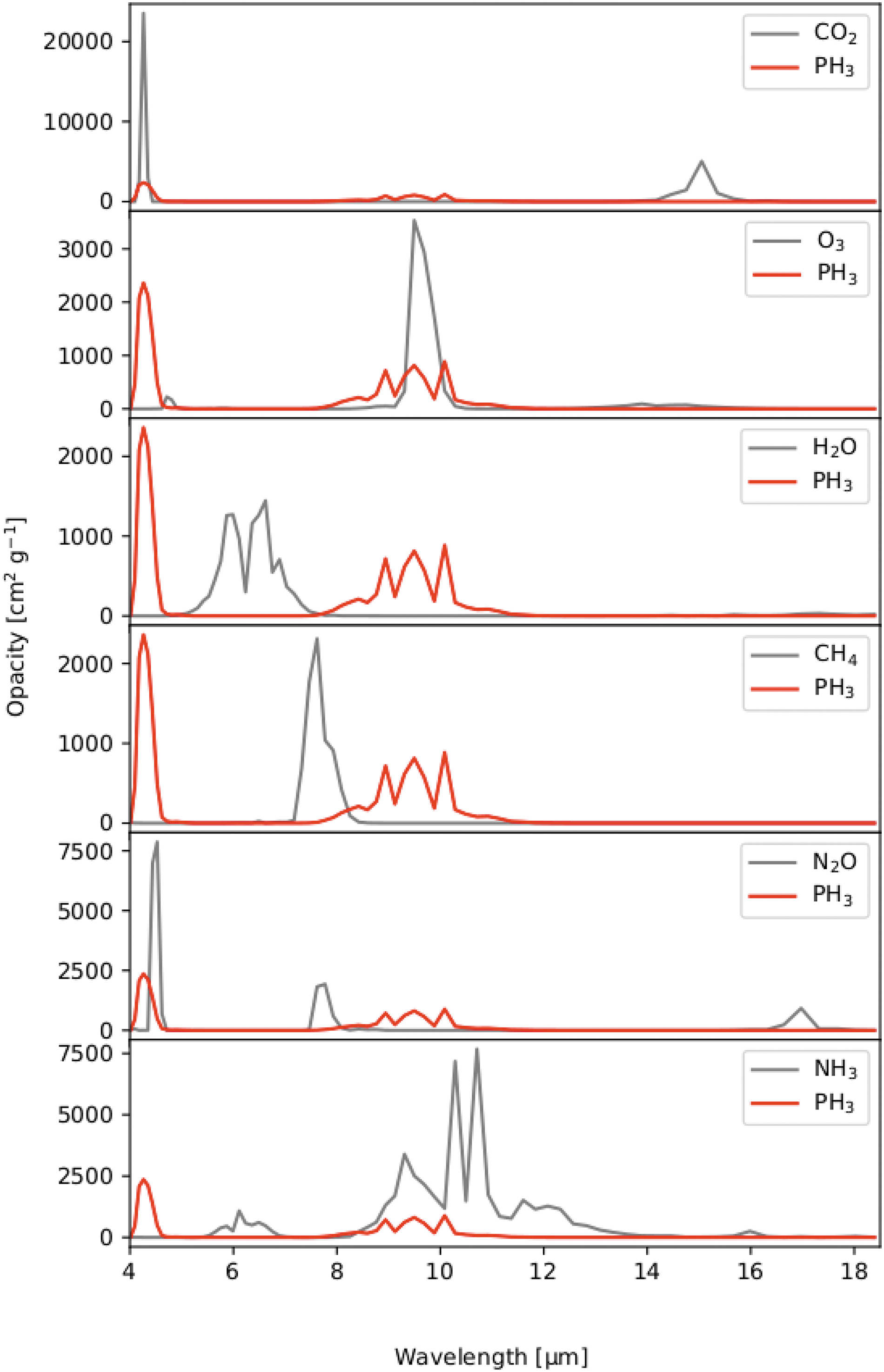
Comparison of the opacities of phosphine with other relevant species in the mid infrared. While some other species are optically active at similar wavelengths, it has a very distinct shape that helps to distinguish it.

2. Modeled Exoplanet Cases

2.1. LIFEsim

For the modeled observations presented here we use LIFEsim, which simulates observations based on a detailed model of an interferometric exoplanet characterization observation and accounts for noise from stellar leakage, local zodiacal, exo-zodiacal, and dust emission, but no instrumental noise (see Dannert et al., 2022).

Following the same approach as Wang et al. (2017) and Sousa-Silva et al. (2020) in their analysis of the observability with JWST, we used LIFEsim to produce synthetic observations of the outlined exoplanet cases with and without phosphine present in their atmospheres. For the presented output spectra, LIFEsim is configured with four apertures of 2 m diameter each, a broadband wavelength range of 4–18.5 μm, and a spectral resolution of R = 50. We assume an exo-zodi level of thrice the local zodi density (following the results from the Hunt for observable signatures of terrestrial systems survey for the expected median level of emission by Ertel et al., 2020) and an interferometric baseline setup between 10 and 100 m (Table 1).

Table 1.
Overview of Simulation Parameters Used in LIFEsim

Parameter Value

Quantum efficiency 0.7

Throughput 0.05

Minimum wavelength 4 μm

Maximum wavelength 18.5 μm

Spectral resolution 50

Imaging baseline 60–600 m

Nulling baseline 10–100 m

Apertures diameter 2 m

Exozodi 3 × local zodi

Parameter	Value
Quantum efficiency	0.7
Throughput	0.05
Minimum wavelength	4 μm
Maximum wavelength	18.5 μm
Spectral resolution	50
Imaging baseline	60–600 m
Nulling baseline	10–100 m
Apertures diameter	2 m
Exozodi	3 × local zodi

These are the same standard values as, for example, used in Quanz et al. (2021).

2.2. Exoplanet models

The main goal of this analysis was to identify the dynamic range of the LIFE observatory's exoplanet characterization potential by testing a few extreme, yet representative, science cases. Fortunately for us the literature already contained studies of phosphine in hot to warm Jupiter sized planets (Wang et al., 2017), as well as various configurations of super-Earths (Sousa-Silva et al., 2020). In our scheme, the Jupiter case represents one of the least challenging types of observations with LIFE, whereas the potentially habitable super-Earth case represents one of the “sweet spots” in terms of instrumental requirements, as well as astrobiologically relevant observations. The additional scenario of the Venus twin was chosen to explore the extreme limits of an experiment like LIFE. The two cases from the literature were modeled with dedicated pipelines tailored to these setups, while the Venus case was modeled with a standard, open (online) tool. In the next subsections, we describe in more detail these pipelines and refer to the original articles and the Planetary Spectrum Generator (PSG) documentation for all specifics. We decided for this approach since it would not have been trivial (or even impossible) to derive all discussed cases from each one or all of the used pipelines. For example, the pipeline of Wang et al. (2017) was optimized for warm Jupiters, while the methods of Sousa-Silva et al. (2020) focused on Super-Earths. Alei et al. (2022) show that even in a full Bayesian retrieval using two different modeling pipelines has only minor impact on the retrieved abundances. Therefore, we assume that this will have little to no effect on the very general feasibility/detectability study we present here. For a more detailed study of the retrieval of chemical and physical properties of an Earth-twin planet that could be obtained with LIFE, we refer to Konrad et al. (2022). The characterization of the main features of an Earth-twin at various stages of its evolution (prebiotic, Great Oxygenation Event, modern atmosphere) is also discussed by Alei et al. (2022).

2.2.1. Venus twin

Within the group of modeled science cases with the LIFE observatory concept, the detection and characterization of a Venus-like planet represent one of the most challenging observations. This case was chosen to explore the edge of the parameter space of possible detections with LIFE. In this study, we test whether our local Solar System science case of potential phosphine in Venus would be detectable remotely. We use models from the PSG (psg.gsfc.nasa.gov; Villanueva et al., 2018; PSG team priv. comms) with a “standard Venus Template” atmosphere and surface (see Table 2 for details) using the built-in “volcanic cloud” model.

Table 2.
Overview of Simulation Parameters Used in the Planetary Spectrum Generator Model of a Venus Twin

Parameter Value

Surface pressure 92 bar

Molecular weight 43.5 g/mol

Gases CO₂, N₂, CO, O₂, SO₂, H₂O, O₃

Phosphine 0 vs. 310 ppm

Clouds PSG “volcanic clouds” model

Surface temperature 756K

Surface gravity 8.87 m/s²

Surface albedo 0.22

Diameter 12,104 km

Host star Sun Twin at 10 pc

Distance to host 0.72 AU

Parameter	Value
Surface pressure	92 bar
Molecular weight	43.5 g/mol
Gases	CO₂, N₂, CO, O₂, SO₂, H₂O, O₃
Phosphine	0 vs. 310 ppm
Clouds	PSG “volcanic clouds” model
Surface temperature	756K
Surface gravity	8.87 m/s²
Surface albedo	0.22
Diameter	12,104 km
Host star	Sun Twin at 10 pc
Distance to host	0.72 AU

PSG = Planetary Spectrum Generator.

We modeled various cases, including 0, 5–20 ppb (the current estimate for Venus from Greaves et al., 2020c) and up to 310 ppm concentration [same as the super-Earth case in Section 2.2.2 from Sousa-Silva et al. (2020), minimum concentration for remote JWST detection there]. For the analysis here, we compare the detectability of the extreme 310 ppm scenario against one without any phosphine.

2.2.2. H₂- and CO₂-dominated super-Earths around M star hosts

The models for the cases of H₂- and CO₂-dominated super-Earths around M star hosts are taken from Sousa-Silva et al. (2020) (Table 3). The atmospheric composition for these scenarios is based on calculations with the photochemical model of Hu et al. (2012) (for more details please see there and references therein). These model super-Earths with radii of 1.75 R_⊕ and masses of 10 M_⊕ are orbiting a 0.26 R_S active 3000K M-dwarf star at 5 pc distance. The assumed phosphine concentrations for the “with PH₃” cases are (H₂-dominated) 220 ppb and (CO₂-dominated) 310 ppm. To maintain equitable, temperate surface conditions (288K), the H₂- and CO₂-dominated cases with no PH₃ emissions are separated from their M dwarf host star by 0.042 and 0.034 AU, respectively. Sousa-Silva et al. (2020) used a photochemical model to explore how PH₃ concentrations responded to two different scenarios: an “active” M-dwarf UV flux model based on observations of GJ1214 and a “quiet” M-dwarf for which the UV fluxes shortward of 300 nm are 0.1% of the “active” scenario fluxes. The “quiet” scenario resulted in PH₃ accumulating to roughly 100 times higher concentrations for the same emission fluxes compared to the “active” M-dwarf scenario. The PH₃ fluxes that would lead to the potential detection of PH₃ are larger than the average terrestrial PH₃ emission estimates, although comparable to the rates at which other biosignature gases are produced, and they are well below observed site-specific PH₃ fluxes on Earth (Sousa-Silva et al., 2020). The reader is directed to the work of Sousa-Silva et al. (2020) for more details on the modeling and the interactions between phosphine and other atmospheric constituents.

Table 3.
Overview of Simulation Parameters Used in the Super Earth Models

Parameters H₂ dominated CO₂ dominated

Surface temperature 288K 288K

Mass 1.75 R_⊕ 1.75 R_⊕

Radius 10 M_⊕ 10 M_⊕

Phosphine 0–220 ppb 0–310 ppm

Host star M star at 5 pc M star at 5 pc

Host star temperature 3000K 3000K

Distance to star 0.042 AU 0.034 AU

Parameters	H₂ dominated	CO₂ dominated
Surface temperature	288K	288K
Mass	1.75 R_⊕	1.75 R_⊕
Radius	10 M_⊕	10 M_⊕
Phosphine	0–220 ppb	0–310 ppm
Host star	M star at 5 pc	M star at 5 pc
Host star temperature	3000K	3000K
Distance to star	0.042 AU	0.034 AU

For more details, see Sousa-Silva et al. (2020).

2.2.3. Warm giant planets around G type hosts

We use models of Wang et al. (2017) (Table 4) for a Jupiter-like planet around a G-type star using chemical kinetics to calculate the abundances of different species, which were then input to the Smithsonian Astrophysical Observatory 1998 radiative transfer code (Kaltenegger and Traub, 2009; Traub and Stier, 1976) to calculate the transmission and emission spectra. Their chemical calculations show that PH₃ is the main phosphorous carrier for exoplanets between 400K and 2000K.

Table 4.
Overview of Model Parameters for Case 3

Parameter Value

Temperature 500K

Radius 1 M_J

Mass 1 R_J

Phosphine 0 vs. solar

Host star G-star at 10 pc

Distance to host star 0.31 AU

Parameter	Value
Temperature	500K
Radius	1 M_J
Mass	1 R_J
Phosphine	0 vs. solar
Host star	G-star at 10 pc
Distance to host star	0.31 AU

“Solar” abundances refer to Asplund et al. (2009).

In these models, the effects of vertical mixing are considered but those of photochemistry in the upper atmosphere of these planets are neglected. The rationale for this is that, while photochemistry is relevant in very hot planets with a hydrogen dominated atmosphere of solar composition close to their stars, their effect on warm planets is limited (e.g., Miguel and Kaltenegger, 2014); in addition, vertical mixing effects are the most relevant ones in the pressures probed by transmission spectroscopy (at the millibar level). Wang et al. (2017) used the solar elemental (atomic) abundances of C, H, O, N, S, and P (Asplund et al., 2009) and let the code calculate the molecules that will be formed given the conditions in the planetary atmosphere calculation. We note that the Wang et al. (2017) calculation was done without considering the effect of photochemistry, which might affect abundances in the upper parts of the atmosphere (pressures <1e⁻⁴ bar) but will most likely have a small effect on the detectability of different species, in particular in MIR emission (vs., e.g., transit transmission in the optical, near infrared).

3. Results

3.1. Estimated yields

In a first step of our study, we checked the availability of potential targets by analyzing the occurrence of the modeled cases in the Solar neighborhood accessible for the theorized observations. Therefore, we checked how many of these potential targets are already known and calculated how many of these LIFE would be able to detect in its detection phase alone even if no other methods would have found those by the time of LIFE's launch.

For the yield simulations, sections of the parameter space that correspond to the described cases are selected. These restrictions to the parameter space are shown in Table 5. We used planet occurrence rates inferred from NASA's Kepler mission to estimate the total expected number of exoplanets in the solar neighborhood and computed the fraction of these, which is detectable with LIFE within 10 h of integration time. For this task, we create synthetic exoplanet populations using the NASA ExoPAG SAG13 occurrence rates (Kopparapu et al., 2018) for all spectral types with P-pop^** (Kammerer and Quanz, 2018) and select different subsamples of planets (Venus twins, super-Earths, and warm Jovians) according to Table 5. For more details on the yield calculations, see Quanz et al. (2022).

Table 5.
Restrictions in Parameter Space for Exoplanet Categories

Parameter Venus twin Super-Earth Warm Jovian

Surface temperature 0.5 R_⊕ <R < 1 R_⊕ 1 R_⊕ <R < 1.75 R_⊕ 6 R_⊕ <R < 14.3 R_⊕

Eq. temperature 200–800K 200–800K (a) 200–800K

Parameter	Venus twin	Super-Earth	Warm Jovian
Surface temperature	0.5 R_⊕ <R < 1 R_⊕	1 R_⊕ <R < 1.75 R_⊕	6 R_⊕ <R < 14.3 R_⊕
Eq. temperature	200–800K	200–800K (a)	200–800K

(a) For the eHZ cases we defined it by the “Recent Venus” and “Early Mars” scenarios for 1 M_⊕ planets from Kopparapu et al. (2014).

For each of these subsamples, we then compute the number of planets which could be detected with an signal-to-noise ratio (SNR) >7 in 10 h of integration time using LIFEsim (Dannert et al., 2022) (we require an SNR >7 to leave a margin for additional instrumental noise). Table 6 shows planets within 20 pc around FGK stars, and Table 7 shows planets within 10 pc around M stars. We limit the M star case to within 10 pc because the survey efficiency (number of detections per observed target) becomes low further out (Quanz et al., 2022). For the case of the super Earth around an M star at 5 pc, the on-sky separation between the planet and its host star lies at 6.8 mas. The detection and characterization of the planet at this close proximity of about 0.3 lambda/B_nulling in terms of the interferometric array properties illustrate the capability of LIFE to directly image close-in targets. This is made possible by the suppression of the central null being a continuous function down to the line-of-sight, which results in the inner working angle of the observatory being a strong function of the target planet luminosity at a fraction of lambda/B_nulling. It should be noted that an absolute lower bound of the inner working angle is given by the fringe spacing due to the imaging baseline, that is, 0.5 lambda/B_imaging.

Table 6.

Number of Potential Targets in the Respective Cases Within 20 pc for FGK Host Stars

Case	Known	Total expected	LIFE detectable
Venus twin	1	247.6 ± 15.7	8.1 ± 3.0
Super-Earth	2	166.8 ± 12.9	44.9 ± 6.9
eHZ super-Earth	0	31.7 ± 5.6	0.5^+0.7 _–0.5
Warm Jovian	13	12.2 ± 3.5	11.9 ± 3.4

Column one shows the planets already known from the NASA Exoplanet Archive, column two the number of planets expected from Kepler statistics (using P-pop with the SAG13 occurrence rates), and column three the number of planets detectable with LIFE within 10 h of integration time.

LIFE = Large Interferometer for Exoplanets.

Table 7.

Same as Table 6 But for M Star Hosts Within 10 pc Only

Case	Known	Total expected	LIFE detectable
Venus twin	0	78.7 ± 8.9	18.5 ± 4.4
Super-Earth	13	53.9 ± 7.3	31.9 ± 6.0
eHZ super-Earth	4	14.0 ± 3.7	4.5 ± 2.0
Warm Jovian	1	1.7 ± 1.3	1.6 ± 1.3

The limits of the “boxes” shown here are taken to be wider than the particular cases described in our examples and are chosen to be aligned with those of Kopparapu et al. (2018). The point we are making is that there will be dozens of planets in this parameter space to explore, which will allow us to derive the presence or nonpresence of phosphine within the order of integration times used in our examples.

3.2. Venus twin

Figure 2 shows the results of a simulated observation of a Venus twin around a Sun twin at 10 pc. We compare a simulated 100 h observation of an atmosphere with 310 ppm of phosphine to a phosphine free model. The significance is only ∼0.15 sigma, and the phosphine is thus not detectable.

FIG. 2.

Detectability of phosphine in the emission spectrum of a Venus Twin planet, after 100 h of observation with LIFE. Top: planet flux for atmospheres with and without PH₃. The blue area represents the 1-σ sensitivity; the gray error bars show an individual simulated observation. Bottom: Statistical significance of the detected difference between an atmospheric model with and without phosphine.

3.3. H₂- and CO₂-dominated super-Earth around M star host

Figures 3 and 4 show the results of simulated observations of H₂- and CO₂-dominated super-Earths orbiting an M star host at 5 pc (from Sousa-Silva et al., 2020; see Section 2.2.2). We modeled a 10 h observation of these atmospheres with 220 ppb and 310 ppm of phosphine, respectively, and compared them to phosphine free models for the same cases. We get a solid detection of up to 5 σ per spectral channel in the bands between 8 and 12 μm that show the biggest difference between a PH₃ bearing atmosphere and one without.

FIG. 3.

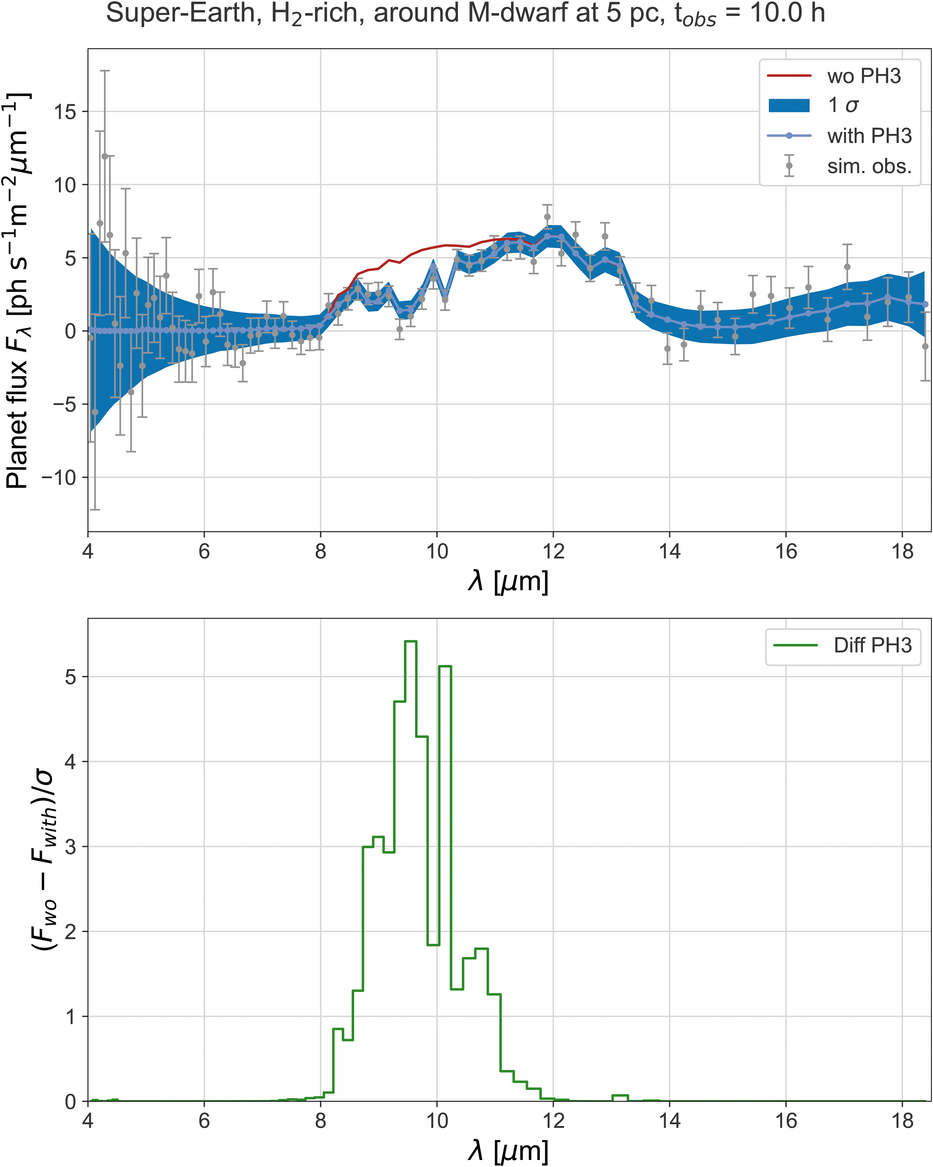
Detectability of phosphine in the emission spectrum of a super Earth exoplanet (10 M_⊕; 1.75 R_⊕) with a hydrogen-rich atmosphere orbiting an active M-dwarf, after 10 h of observation with LIFE. Top: planet flux for atmospheres with and without PH₃, respectively; blue and red curves represent a modeled atmosphere with a PH₃ mixing ratio of 310 ppm and an atmosphere without PH₃. The blue area represents the 1-σ sensitivity; the gray error bars show an individual simulated observation. Bottom: Statistical significance of the detected difference between an atmospheric model with and without phosphine.

FIG. 4.

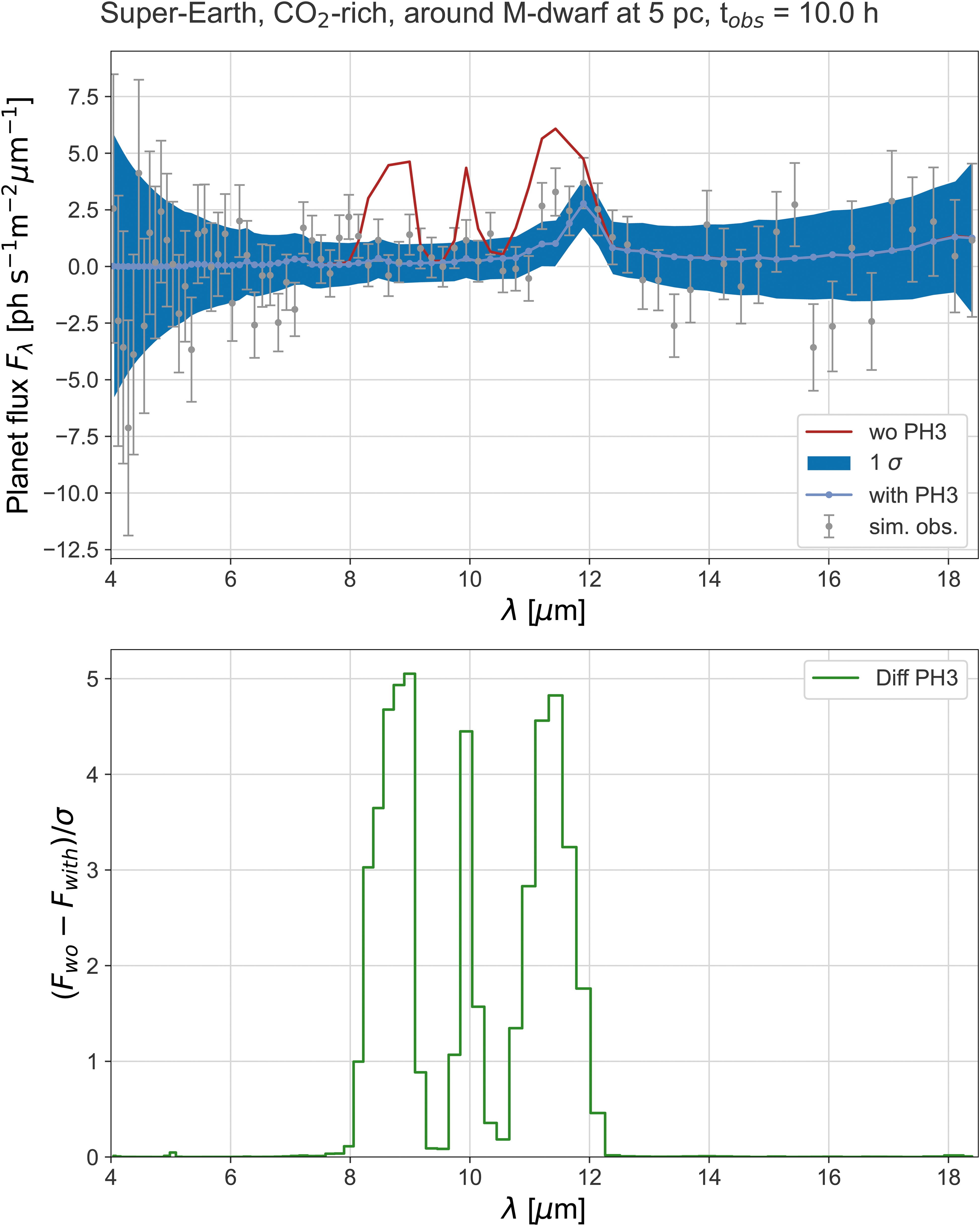
Detectability of phosphine in the emission spectrum of a super Earth exoplanet (10 M_⊕; 1.75 R_⊕) with a carbon dioxide-rich atmosphere orbiting an active M-dwarf, after 10 h of observation with LIFE. Top: planet flux for atmospheres with and without PH₃, respectively; blue and red curves represent a modeled atmosphere with a PH₃ mixing ratio of 310 ppm and an atmosphere without PH₃. The blue area represents the 1-σ sensitivity; the gray error bars show an individual simulated observation. Bottom: Statistical significance of the detected difference between an atmospheric model with and without phosphine.

3.4. 500K giant around G star host

Figure 5 shows the results of a simulated observation of a 500K giant planet orbiting at G star at 10 pc. We get a very solid detection of up to 50 σ per spectral channel in the band around 4.5 μm and up to 20 σ per spectral channel in the bands between 8 and 12 μm that show the biggest difference between a PH₃ bearing atmosphere and one without.

FIG. 5.

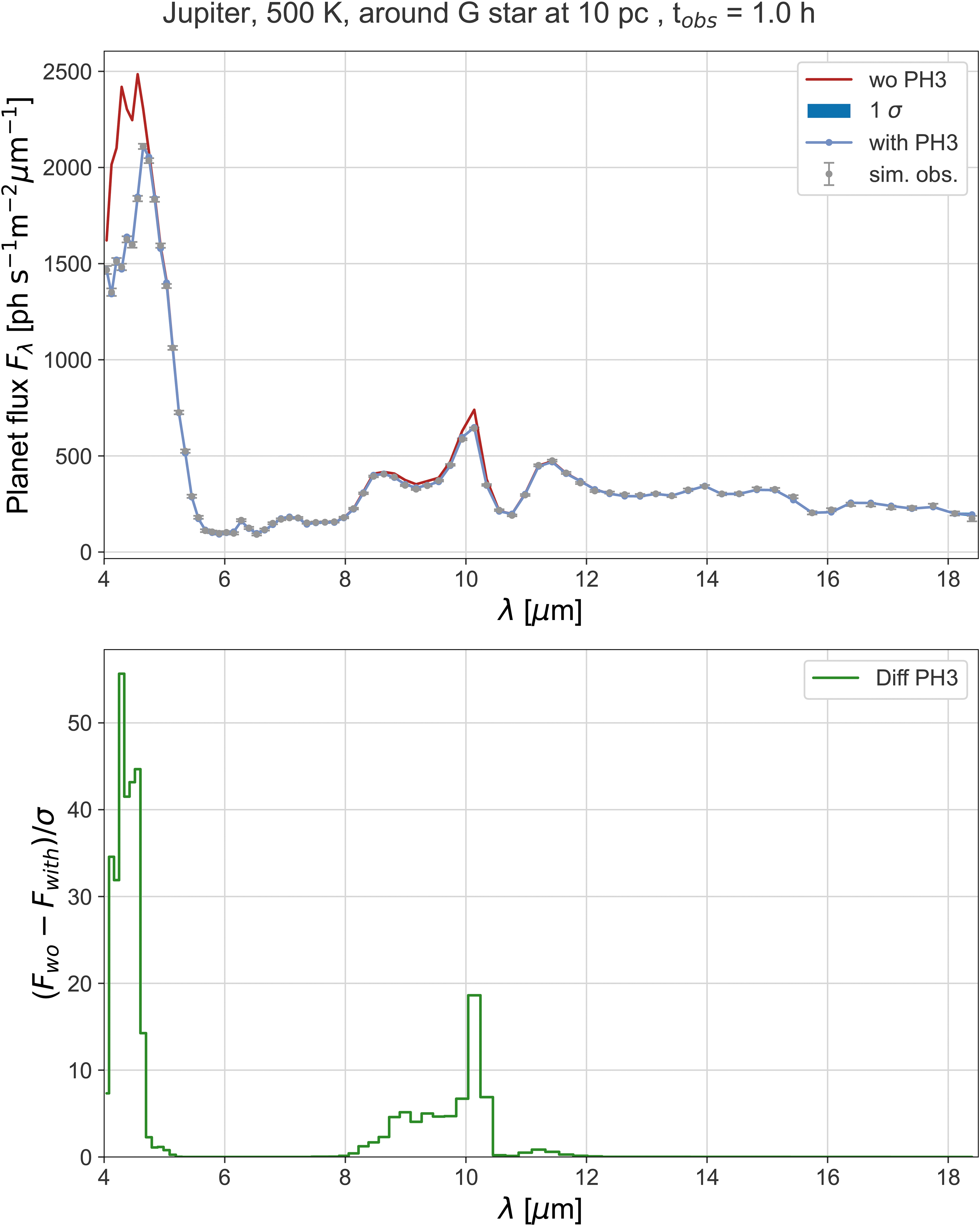
Detectability of phosphine in the emission spectrum of 500K warm Jupiter like planet, after 1 h of observation with LIFE. Top: planet flux for atmospheres with and without PH₃. The blue area represents the 1-σ sensitivity; the gray error bars show an individual simulated observation. Bottom: Statistical significance of the detected difference between an atmospheric model with and without phosphine.

4. Discussion and Conclusions

By applying a detailed mission and instrument simulator for a future MIR space interferometer to map the detectability space of phosphine in three different, extreme planet types and scenarios we find the following:

Observations of extrasolar PH₃ in a Venus-like planet around G-type stars are very challenging. Even after 100 h of simulated observation, the difference in two extreme forward models (no vs. 310 ppm of PH₃) of phosphine is not detectable.

For the cases of H₂ and CO₂ dominated super-Earths around M star hosts, a mission like LIFE can produce highly informative observations in a relatively small amount of time. Applied to a suite of models for these planets taken from the literature, LIFEsim confirms that phosphine concentrations of 220 ppb (H₂ case) and 310 ppm (CO₂ case) can clearly be distinguished from PH₃ free atmospheres with integration times in the order of 10 h.

Giant planets, such as the example of the 500K Jupiter, can quickly and easily be characterized in the order of 1 h. LIFE will allow us to make—if present—detections of phosphine in many giant exoplanets and help understand its relevance and occurrence.

In Table 8, we show a comparison of the observation times needed to get a significant detection of phosphine in the described cases. In comparison to the studies of JWST observability of the same scenarios at comparable signal to noise ratios of Sousa-Silva et al. (2020) and Wang et al. (2017), we can report that a concept like LIFE will perform more than an order of magnitude faster: the super-Earths scenarios take 131 h (for a H₂-dominated atmosphere) and 48 h (for a CO₂-dominated atmosphere) of JWST secondary eclipse emission spectrophotometry (Sousa-Silva et al., 2020) in comparison to about 10 h of observation time needed with LIFE. While the warm Jupiter scenario of Wang et al. (2017) is observable only in transit transmission spectrophotometry within about 30 h of time with JWST, it takes only 1 h with LIFE for a solid detection of phosphine. It is also important to note that the JWST observations require multiple visits to add up the times from a number of eclipse/transit events, while the LIFE observation can be done in a single visit and on nontransiting systems as well.

Table 8.

Overview of Observation Times Needed to Detect the Modeled Levels of PH₃

Observation type	500K giant (hours)	H₂ super Earth (hours)	CO₂ super Earth (hours)
JWST transit/transmission spectrophotometry	∼29	∼91	>200
JWST eclipse/emission spectrophotometry	>30	∼131	∼48
LIFE nulling interferometry/emission spectroscopy	<1	<10	<10

JWST numbers from Wang et al. (2017) and Sousa-Silva et al. (2020).

JWST = James Webb Space Telescope.

A caveat of the presented analysis is that it was done for presumably extreme cases and for the comparison of forward models with and without phosphine in the respective atmospheres. Therefore, the next steps for us will be to simulate more examples and run full Bayesian retrievals to get to more quantitative assessments also on the limits of phosphine detectability. The analysis presented here will help to prioritize the parameter range to go for in the next deeper dives into these atmospheres with more detailed retrieval simulations. These results will inform crucial questions and decisions in the early design phase of a mission like LIFE. In combination with other early results of the LIFE initiative, these results will help to get a better idea on how to handle the overall planet statistics in the planning phase of large future missions for terrestrial exoplanet characterization by giving a first order estimate of the realistically explorable parameter space. To build upon these estimates, the LIFE team is currently working on a comprehensive simulation of the consequences on scheduling for the survey and characterization phases of the LIFE mission. At this end, we are also investigating novel machine learning methods that are necessary to expand and augment our front-to-end simulations of the full LIFE survey, including full retrievals (see, e.g., Gebhard et al., 2022). These results will deliver timely information needed for the early definition of sensitivity, wavelength coverage, and spectral resolution requirements on the technology side and set important limits for the modelers to reduce the computing load for upcoming future work such as calculations of spectral/photochemical grids.

Footnotes

Acknowledgments

The authors thank the referees, as well as the participants, of AbSciCon 2022 for very useful feedback on this work.

Authors' Contributions

D.A.: Conceptualization, methodology, data curation, writing-original draft, writing-review and editing, visualization, supervision, project administration. M.O.: Software, methodology, visualization. F.D.: Software, methodology, formal analysis, data curation. Y.M. and C.S.S.: Methodology, writing-review and editing. J.K.: Methodology, software, formal analysis, writing-review and editing. F.M., B.S.K., and H.S.W.: Writing-review and editing. E.A.: Writing-review and editing, visualization. S.P.Q.: Writing-review and editing, supervision.

Author Disclosure Statement

No competing financial interests exist.

Funding Information

Part of this work was supported by SNF, NCCR PlanetS, and the Heising-Simons Foundation.

Abbreviations Used

References

Akins

, Lincowski

, Meadows

, et al. Complications in the ALMA Detection of Phosphine at Venus. ApJL, 2021; 907:L27; doi: 10.3847/2041-8213/abd56a

Alei

, Konrad

, Angerhausen

, et al. Large Interferometer For Exoplanets (LIFE): V. Diagnostic potential of a mid-infrared space-interferometer for studying Earth analogs. Astron Astrophys, 2022; 665:A106; doi: 10.1051/0004-6361/202243760

Asplund

, Grevesse

, Sauval

, et al. The chemical composition of the sun. Annu Rev Astron Astrophys, 2009; 47:481–522; doi: 10.1146/annurev.astro.46.060407.145222

Bains

, Petkowski

, Seager

, et al. Phosphine on venus cannot be explained by conventional processes. Astrobiology, 2021; 21(10):1277–1304; doi: 10.1089/ast.2020.2352

Ben-Ami

, López-Morales

, Szentgyorgyi

In Ground-based and Airborne Instrumentation for Astronomy VII. SPIE Conf Ser, 2018; 10702:107026N; doi: 10.1051/0004-6361/201935302

Bregman

, Lester

, Rank

Observations of the v₂ band of PH₃ in the atmosphere of Saturn. ApJ, 1975; 202:L55; doi: 10.1086/181979

Dannert

, Ottiger

, Quanz

, et al. Large Interferometer For Exoplanets (LIFE)—II. Signal simulation, signal extraction, and fundamental exoplanet parameters from single-epoch observations. Astron Astrophys, 2022; 664:A22; doi: 10.1051/0004-6361/202141958

Des Marais

, Harwit

, Jucks

, et al. Remote sensing of planetary properties and biosignatures on extrasolar terrestrial planets. Astrobiology, 2002; 2:153; doi: 10.1089/15311070260192246

Encrenaz

, Greathouse

, Marcq

, et al. A stringent upper limit of the PH₃ abundance at the cloud top of Venus. Astron Astrophys, 2020; 643:L5; doi: 10.1051/0004-6361/202039559

10.

Ertel

, Defrère

, Hinz

, et al. The HOSTS Survey for Exozodiacal Dust: Observational results from the complete survey. Astron J, 2020; 159:177; doi: 10.3847/1538-3881/ab7817

11.

Fletcher

, Orton

, Teanby

, et al. Phosphine on Jupiter and Saturn from Cassini/CIRS. Icarus, 2009; 202:543–564; doi: 10.1016/j.icarus.2009.03.023

12.

Fujii

, Angerhausen

, Deitrick

, et al. Exoplanet biosignatures: Observational prospects. Astrobiology, 2018; 18:739; doi: 10.1089/ast.2017.1733

13.

Gaudi

, Seager

, Mennesson

, et al. The Habitable Exoplanet Observatory (HabEx) mission concept study final report. arXiv:2001.06683; 2020.

14.

Gebhard

, Angerhausen

, Alei

, et al. Using machine learning to parameterize pressure-temperature profiles for atmospheric retrievals of exoplanets. In: 2022 Astrobiology Science Conference. AGU; 2022.

15.

Greaves

, Bains

, Petkowski

, et al. On the robustness of phosphine signatures in Venus' clouds. Nat Astron, 2021b;5:726–728; doi: 10.1038/s41550-021-01423-y

16.

Greaves

, Richards

AMS

, Bains

, et al. Re-analysis of phosphine in Venus' clouds. Nat Astron, 2021a;5:636–639; doi: 10.1038/s41550-021-01424-x

17.

Greaves

, Richards

AMS

, Bains

, et al. Phosphine gas in the cloud decks of Venus. Nat Astron, 2020; 5:655–664; doi: 10.1038/s41550-020-1174-4

18.

, Seager

, Bains

Photochemistry in Terrestrial Exoplanet Atmospheres. I. Photochemistry model and benchmark cases. ApJ, 2012; 761:166; doi: 10.1088/0004-637X/761/2/166

19.

Kaltenegger

, Traub

. Transits of earth-like planets. ApJ, 2009; 698:519; doi: 10.1088/0004-637X/698/1/519

20.

Kammerer

, Quanz

. Simulating the exoplanet yield of a space-based MIR interferometer based on Kepler statistics. Astron Astrophys, 2018; 609:A4; doi: 10.1051/0004-6361/201731254

21.

Konrad

, Alei

, Angerhausen

, et al. Large Interferometer For Exoplanets (LIFE): III. Spectral resolution, wavelength range and sensitivity requirements based on atmospheric retrieval analyses of an exo-Earth. Astron Astrophys, 2022; 664:A23; doi: 10.1051/0004-6361/202141964

22.

Kopparapu

, Hébrard

, Belikov

, et al. Exoplanet classification and yield estimates for direct imaging missions. ApJ, 2018; 856:122; doi: 10.3847/1538-4357/aab205

23.

Kopparapu

, Ramirez

, Schottel Kotte

, et al. Habitable zones around main-sequence stars: Dependence on planetary mass. ApJ, 2014; 787:L29; doi: 10.1088/2041-8205/787/2/L29

24.

Krissansen-Totton

, Olson

, Catling

. Disequilibrium biosignatures over Earth history and implications for detecting exoplanet life. Sci Adv, 2018; 4:eaao5747; doi: 10.1126/sciadv.aao5747

25.

Larson

, Treffers

, Fink

Phosphine in Jupiter's atmosphere: The evidence from high-altitude observations at 5 micrometers. Astron J, 1977; 211:972; doi: 10.1086/155009

26.

Lincowski

, Meadows

, Crisp

, et al. Claimed detection of PH₃ in the clouds of Venus is consistent with mesospheric SO2. ApJL, 2021; 908:L44; doi: 10.3847/2041-8213/abde47

27.

Lovis

, Snellen

, Mouillet

, et al. Atmospheric characterization of Proxima b by coupling the SPHERE high-contrast imager to the ESPRESSO spectrograph. Astron Astrophys, 2017; 599:A16; doi: 10.1051/0004-6361/201629682

28.

Meixner

, Cooray

, Leisawitz

, et al. Origins Space Telescope Mission Concept Study Report. arXiv:1912.06213; 2019.

29.

Miguel

, Kaltenegger

Exploring atmospheres of hot mini-Neptunes and extrasolar giant planets orbiting different stars with application to HD 97658b, WASP-12b, CoRoT-2b, XO-1b, and HD 189733b. ApJ, 2014; 780:166; doi: 10.1088/0004-637X/780/2/166

30.

Quanz

, Absil

, Angerhausen

, et al. Atmospheric characterization of terrestrial exoplanets in the mid-infrared: Biosignatures, habitability, and diversity. arXiv:1908.01316; 2019; doi: 10.1007/s10686-021-09791-z

31.

Quanz

, Kammerer

, Defrère

, et al. Exoplanet science with a space-based mid-infrared nulling interferometer. SPIE, 2018; 10701:107011I; doi: 10.1117/12.2312051

32.

Quanz

, Ottiger

, Fontanet

, et al. Large Interferometer For Exoplanets (LIFE). I. Improved exoplanet detection yield estimates for a large mid-infrared space-interferometer mission. Astron Astrophys, 2022; 664:A21; doi: 10.1051/0004-6361/202140366

33.

Schwieterman

, Kiang

, Parenteau

, et al. Exoplanet Biosignatures: A review of remotely detectable signs of life. Astrobiology, 2018; 18:663; doi: 10.1089/ast.2017.1729

34.

Seager

, Bains

, Petkowski

. Toward a list of molecules as potential biosignature gases for the search for life on exoplanets and applications to terrestrial biochemistry. Astrobiology, 2016; 16:465; doi: 10.1089/ast.2015.1404

35.

Snellen

IAG

, de Kok

, le Poole

, et al. Finding extraterrestrial life using ground-based high-dispersion spectroscopy. ApJ, 2013; 764:182; doi: 10.1088/0004-637X/764/2/182

36.

Snellen

IAG

, Guzman-Ramirez

, Hogerheijde

, et al. Re-analysis of the 267-GHz ALMA observations of Venus: No statistically significant detection of phosphine. Astron Astrophys, 2020; 644:L2; doi: 10.1051/0004-6361/202039717

37.

Sousa-Silva

, Seager

, Ranjan

, et al. Phosphine as a biosignature gas in exoplanet atmospheres. Astrobiology, 2020; 20:235; doi: 10.1089/ast.2018.1954

38.

The LUVOIR Team. The LUVOIR Mission Concept Study Final Report. arXiv:1912.06219; 2019; doi: 10.48550/arXiv.1912.06219

39.

Thompson

MA.

The statistical reliability of 267 GHz JCMT observations of Venus: No significant evidence for phosphine absorption. MNRAS, 2021; 501:L18; doi: 10.1093/mnrasl/slaa187

40.

Tinetti

, Drossart

, Eccleston

, et al. A chemical survey of exoplanets with ARIEL. Exp Astron, 2018; 46:135; doi: 10.1007/s10686-018-9598-x

41.

Traub

, Stier

. Theoretical atmospheric transmission in the mid-and far-infrared at four altitudes. Appl Opt, 1976; 15:364; doi: 10.1364/AO.15.000364

42.

Trompet

, Robert

, Mahieux

, et al. Phosphine in Venus' atmosphere: Detection attempts and upper limits above the cloud top assessed from the SOIR/VEx spectra. Astron Astrophys, 2021; 645:L4; doi: 10.1051/0004-6361/202039932

43.

Villanueva

, Cordiner

, Irwin

, et al. No evidence of phosphine in the atmosphere of Venus from independent analyses. Nat Astron, 2021; 5:631–635; doi: 10.1038/s41550-021-01422-z

44.

Villanueva

, Smith

, Protopapa

, et al. Planetary spectrum generator: An accurate online radiative transfer suite for atmospheres, comets, small bodies and exoplanets. J Quant Spectr Rad Transf, 2018; 217:86; doi: 10.1016/j.jqsrt.2018.05.023

45.

Visscher

, Lodders

, Fegley Jr

Atmospheric chemistry in giant planets, brown dwarfs, and low-mass dwarf stars. II. Sulfur and phosphorus. ApJ, 2006; 648:1181; doi: 10.1086/506245

46.

Wang

, Miguel

, Lunine

Modeling synthetic spectra for transiting extrasolar giant planets: Detectability of H₂S and PH₃ with JWST. ApJ, 2017; 850:199; doi: 10.3847/1538-4357/aa978e

47.

Weisstein

, Serabyn

Submillimeter Line Search in Jupiter and Saturn. Icarus, 1996; 123:23; doi: 10.1006/icar.1996.0139

48.

Wunderlich

, Scheucher

, Grenfell

, et al. Detectability of biosignatures on LHS 1140 b. Astron Astrophys, 2021; 647:A48; doi: 10.1051/0004-6361/202039663

Large Interferometer for Exoplanets: VIII. Where Is the Phosphine? Observing Exoplanetary PH 3 with a Space-Based Mid-Infrared Nulling Interferometer

Abstract

1. Introduction

2.1. LIFEsim

Table 1. Overview of Simulation Parameters Used in LIFEsim Parameter Value Quantum efficiency 0.7 Throughput 0.05 Minimum wavelength 4 μm Maximum wavelength 18.5 μm Spectral resolution 50 Imaging baseline 60–600 m Nulling baseline 10–100 m Apertures diameter 2 m Exozodi 3 × local zodi

2.2.1. Venus twin

Table 4. Overview of Model Parameters for Case 3 Parameter Value Temperature 500K Radius 1 MJ Mass 1 RJ Phosphine 0 vs. solar Host star G-star at 10 pc Distance to host star 0.31 AU

3.1. Estimated yields

Table 5. Restrictions in Parameter Space for Exoplanet Categories Parameter Venus twin Super-Earth Warm Jovian Surface temperature 0.5 R⊕ <R < 1 R⊕ 1 R⊕ <R < 1.75 R⊕ 6 R⊕ <R < 14.3 R⊕ Eq. temperature 200–800K 200–800K (a) 200–800K

Footnotes

Acknowledgments

Authors' Contributions

Author Disclosure Statement

Funding Information

Abbreviations Used

References

Table 4.
Overview of Model Parameters for Case 3

Parameter Value

Temperature 500K

Radius 1 M_J

Mass 1 R_J

Phosphine 0 vs. solar

Host star G-star at 10 pc

Distance to host star 0.31 AU

Table 5.
Restrictions in Parameter Space for Exoplanet Categories

Parameter Venus twin Super-Earth Warm Jovian

Surface temperature 0.5 R_⊕ <R < 1 R_⊕ 1 R_⊕ <R < 1.75 R_⊕ 6 R_⊕ <R < 14.3 R_⊕

Eq. temperature 200–800K 200–800K (a) 200–800K