




Abstract
Future systems of extreme isolation, including initiatives in space exploration, may require the services of onboard ecosystems. Biosphere 2, which ran between 1991 and 1993, aspired to mimic the earthly ecosystem and assess the ability of humans and other species to survive in a fully enclosed space. In this study, the data for plant species survival in the tropical rainforest sector from the first 2-year mission were studied through the prism of the neutral theory of biodiversity (NTB), which predicts how closed communities develop and how they lose species due to random demographic effects. Biosphere-2 lost species faster than a neutral process would predict. The specific reasons have been well documented, but the integrated approach of NTB offers new insights. It predicts that a closed ecological community must lose species and there is a specific time frame for this. To test it properly, the operation time of Biosphere-2 should have been at least 30 times greater. The new insights that NTB brings to the story of Biosphere 2 could be important for microcosm studies in general. A similar analysis suggests that the operation and testing time of other simulated ecosystems should also be increased.
Introduction
The ability of living organisms to survive and reproduce in ever-changing and adverse conditions needs to be studied not only for the sake of understanding the effects of human activities on Earth's environment but also for the rising prospects of space colonization. To do so, the individual functions and collaboration between ecosystems should be looked at on a smaller scale that enables the control of the different factors involved. Such study should be conducted in conditions of isolation to minimize any contact with the external environment.
A common approach has been construction of artificial ecosystems that vary in size. These experimental structures usually reproduce the exact conditions of a specific ecosystem, including its biotic and abiotic factors (Matheson, 2008). Examples of such systems are ecotrons, which are usually multiple identical facilities that enable the study of specific interactions (Roy et al., 2021). Aquaria are another form of closed ecosystems that can vary greatly in their volume and capacity.
Many approaches have essentially followed an agricultural paradigm, beginning with a small number of crop species. However, some projects have attempted to construct and run autonomous ecological communities. This makes sense because most real agricultural systems are embedded within ecosystems that provide services such as pollination and soil quality, so some degree of ecological autonomy is going to be necessary.
One of the most ambitious large-scale efforts to mimic and understand ecosystem interactions in closed ecosystems was the famous Biosphere 2 experiment, a closed facility of size 1.28 ha, designed to sustain life for about 100 years (Walter and Carmen Lambrecht, 2004). Biosphere 2 could host an eight-person crew (the “Biospherians”), isolated in the sealed structure and sustained by it, producing their own food.
It had seven different compartments, five of which constituted the wilderness areas (savannah, oceanic ecosystem, desert, mangrove marshland, and tropical rainforest). The remaining areas were an intensive agriculture space for food production and a habitable region where Biospherians resided. Additionally, the experiment included two separate chambers that were able to adjust their volume to keep the temperature constant and to keep humidity in equilibrium (Nelson et al., 1992).
The first mission took place between 1991 and 1993 and lasted 2 years in total. Despite careful preparation and extensive efforts to predict the overall operation of the system, the mission encountered many serious problems. The most striking and important one seems to be reduction in the concentration of oxygen, which fell from 20.9% when the enclosure started to 14.4% about 16 months later. This malfunction was attributed to lack of equilibrium between photosynthetic oxygen production and its consumption by respiration.
Other problems included the loss of pollinators, algal mats in the oceanic biome that had to be removed manually, and certain plant species that dominated over edible crops and trees (Cohen and Tilman, 1996; Dempster, 2008). The lack of previous results from such large-scale experiments made difficult any prediction of what was to follow. One of the most influential factors is considered the choice of nutrient-rich soil. The amounts of different elements appear to be far from normal and may have led to a rapid imbalance shortly after the experiment started.
The presence of pests combined with the reduced solar irradiation available through the glass panels caused low yields and therefore food scarcity. Along with this, the huge number of species selected and their mixture in different artificial communities probably changed their function and led to their quick degradation (Walter and Carmen Lambrecht, 2004; Milçu et al., 2011). One of the most affected biomes of Biosphere 2 was the tropical rainforest, which hosted a great variety of plants, but lost more than half of the identified plant individuals by the end of the enclosure 2 years later (Leigh et al., 1999).
Evidently this quick loss of species and individuals does not correspond to the natural rates of species loss. To get some perspective on its performance relative to a natural community of the same size, we employed a neutral community concept. A well-known ecological theory for development of an ecological community in isolation is the neutral theory of biodiversity (NTB) (Hubbell, 2001). One of the crucial aspects of this theory is the assumed neutrality at the species level.
This theory has been used to study the loss of species in naturally isolated systems such as birds on islands (Halley and Iwasa, 2011) and plants on habitat fragments (Gilbert et al., 2006). The results have been sufficiently close to observations to make this a plausible model for other applications. Applying this model to a potential space colony brings an important perspective. Thus, in this work, we have tried to simulate and predict what would be the expected plant succession timeline if the organisms of the tropical rainforest's biome were living under a neutral equilibrium.
Our main objective is to use NTB to examine whether the observed loss of species could be attributed to neutral drift or whether we must consider other causes. These findings could thus help us better understand the actual rapid loss of species in Biosphere 2's 2 years of operation that fell so short of Biosphere 2's original ambitious aims of maintaining a free-standing community for 100 years. It can therefore enhance our ability to assess the performance of closed ecosystems intended to survive a long time.
Methods
Data sources
For the study of plants that constituted the tropical rainforest biome of Biosphere 2, we selected the data presented by Leigh et al. (1999). At the time of the experiment, some plant species were known, while others were not fully identified (i.e., only family or/and genus were known, although they were recorded in the species catalog) or not identified at all. In the present study, we chose to work only with the fully or partially identified plants, which belong to 342 species groups and include, in total, 1571 individuals. The abundance levels of each initial species group were transcribed and classified in an EXCEL sheet.
After consulting the TRY plant database (Kattge et al., 2020) for the average lifetime of the plants used in the tropical rainforest biome, we found that most of the fully known species were perennials—mainly trees, lianas, and vines. The lifetimes of 10 different perennial plant species were selected to find the average lifetime.
The fully identified species in the biome were 282 in total and therefore our species' lifetime assessment has taken into consideration ∼3.6% of the known plant species. At this point, it needs to be stressed that at the time this work was written, no other database was found with availability of plant lifetimes. The data concerning species lifetimes are presented in Supplementary Table S1.
Through this assessment, the average lifetime value found is 37.1 years and in that time frame, we therefore expect most of the initial plants to have died and be succeeded by the next plant generation. Many perennial plants and especially trees have longer lifetimes, but here we accept that the above value is indicative of the Biosphere 2 tropical plants' average lifetimes.
In this work, we introduce the concept of generation time, which corresponds to the time needed for half of the plants to be replaced. For the purposes of this work, we assume that the generation time is half the average lifetime, that is, ∼18.5 years.
Theoretical background
The unified neutral theory of biodiversity and biogeography (UNTB), which was proposed by Stephen Hubbell, is a model of ecological communities under speciation and extinction and seeks to explain the existence of species richness and relative species abundance through the lens of neutral equilibrium (Hubbell, 2001). Species are assumed not to interact as predators, parasites, or mutualists, but only interact through competition for space.
According to this theory, each organism belonging in a certain community is assumed (on a per capita basis) to be equal with the rest and thus neutrality is ensured. One of the most important aspects of this theory is that in a closed community with no immigration and with equal chances of death and birth of each species, zero-sum dynamics is in force.
In other words, there is no increase in a species' abundance without another one decreasing, and the total number of individuals in the community remains invariant. Thus, there is a probability of any species going extinct if its abundance is low and so every community will tend to lose species, especially if the community is small. In Hubbell's 2001 NTB, biodiversity is maintained by a nonzero speciation rate.
A fully closed local community, such as the tropical rainforest biome of Biosphere 2, is a small community that operates for a relatively short period of time (not an evolutionary timescale), so we expect speciation to be effectively absent. For this community, we can apply a simpler NTB without speciation (Hubbell, 2001).
Two important factors define the behavior of this community: the size and the distribution of abundance of species in the community. The initial abundance of the focal species in the community influences to a great extent the time needed for it to either go extinct or become the only dominant species. The smaller the community, the quicker the species loss and drift toward monodominance.
To test the accuracy of results obtained from the tropical rainforest data processing with NTB, we used the equation of Halley and Iwasa (2011), as given below, for the number of species at time t after isolation:
In this equation, the species richness for each specific time step is given as a function of time in years, S
0 is the initial species richness and t
50 is the half-life (i.e., time needed for the initial species richness to become exactly half). Also from Halley and Iwasa (2011), half-life can be derived from the following equation:
The terms of the equation are the years of life per generation (τ), corresponding to the actual generation time found to be ∼18.5 years, as referred above; the initial number of individuals (N); and the initial species richness (S 0).
In this work, we have converted the equation into linear form to find the best fit using the least squares method to obtain the values of S 0 and t 50. We also used Equation (2) along with the known input values to assess the evolution of the neutral community. In this way, two different lines emerge, which are compared with the one produced by the NTB simulation model.
The simulation scripts were written in R and are available in the Supplementary Data. The routine was developed with commands from the UNTB package by Hankin (2007). The command “untb” that simulates random drift has been the main constituent of the work. The input for the command was the initial number of species and the individuals assigned to each one of them and the number of deaths per generation, which corresponds to 785 (i.e., half of the initial plant individuals).
The command was then encapsulated in a bigger loop that ran until the number of the remaining species was reduced to a specific value. The value was decided each time based on the chosen percentage of remaining species (i.e., 308 when 90% of the initial species are still present). The number of generations to reach this number of species is equivalent to the loop repetition counts. The generations needed to reach the species richness percentages retained are presented in Supplementary Table S2. For each of these remaining species values, the routine was repeated 1000 times.
After running the routine, we used the five-number summary method (minimum value, lower quartile value, median value, upper quartile value, and maximum value) to check the generations needed to reach each remnant species' richness percentage. Afterward, the acquired data were plotted and are presented in the Results section that follows below. In the second part of our analysis, we fitted our results to the equation by Halley and Iwasa [Eq. (1), above], as mentioned previously.
The linear fit and its accuracy were then tested statistically with R.
Species loss in a population decline
In the running of the neutral model, it is assumed that the population stays constant. However, in the Biosphere 2 experiment, only 744 from the initial 1571 individuals were still surviving by the time it was shut down. This, by itself, if done in a purely random way, would cause the stochastic extinction of several species. Could this be an alternative explanation for the observed loss of species observed at the end of Biosphere 2's 2-year enclosure?
To test this, we randomly sampled individuals from the initial pool of species and assessed whether the results of our sampling match the actual species loss in Biosphere 2. We iterated the random sampling procedure 10,000 times in total.
Results
Simulated persistence times and comparison with the NTB
After introducing into the routine the specific species richness milestone steps described previously, we iterated the code 1000 times per step. The five-number summary for the resulting generation times per step is presented in Supplementary Table S3. To assess the agreement of our findings with other neutral models, we fitted our results in the equation by Halley and Iwasa (2011).
The data were fitted in two ways. In the first case, the terms of the equation are considered known. These are the years of life per generation (τ), corresponding to the actual generation time found to be ∼18.5 years, as mentioned previously; the initial number of individuals (N = 1571); and the initial species richness (S 0 = 342). By inserting the above values into the equation for the community half-life, we find that it is equal to ∼170 years.
In the second case, both half lifetime and initial species richness were considered unknown and attempted to be determined by linear fit with the least squares method. For this reason, the generation time was converted into years. The data for the fit is presented in Supplementary Table S4. The value of half lifetime (t 50) was found to be ∼409 years (408.72 years) and the initial species' richness (S 0) was ∼196 species (195.73 species).
To check our model's accuracy, we calculated the multiple and adjusted R 2 values, which are 0.9962 and 0.9960, respectively (p-value <2.2 × 10⁻¹⁶). The comparison of lines that occur from these two fitting attempts, along with simulation results for the median amount of time needed to reach the remaining species' richness percentage milestones, is presented in Supplementary Fig. S1.
The simulation results for the maximum, minimum, and median time corresponding to each species richness percentage step along with the results from the equation fit described in the first case were plotted and are presented in Fig. 1, where the time axis is logarithmic, and its value is set in years (generation time = 18.5 years). The pattern of the lines indicates that species abundance initially declines quickly, but later larger persistence times prevail as the line slope becomes smaller.
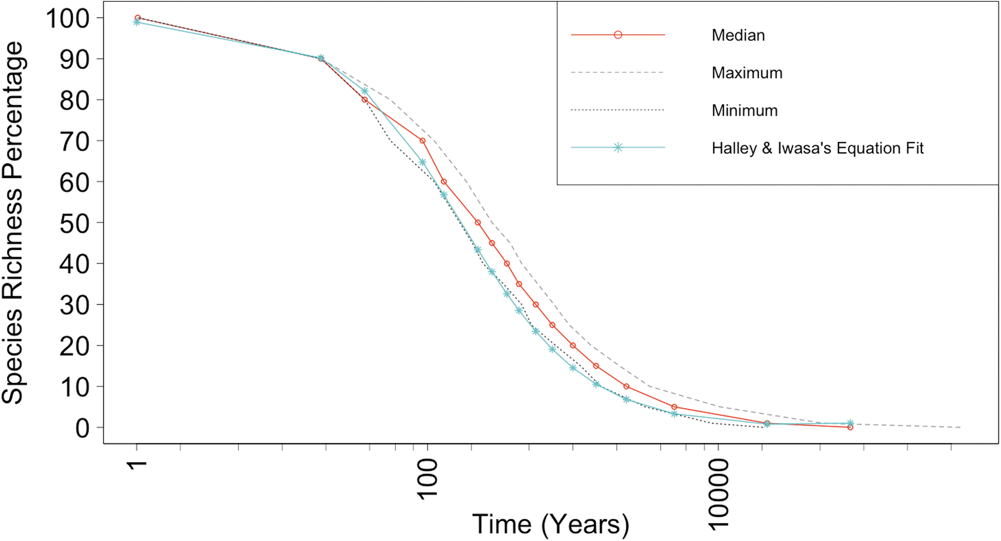
Species richness retained along with time. Each line represents the percentage of species richness that is retained along with years (generation time × 18.5 years). The lower broken gray line represents the minimum number of generations until each species richness percentage is reached, the red line represents the median generation number, and the upper broken gray line represents the maximum. Color graphics are available online.
This increase in persistence time becomes extremely large by the time only 10% species richness is left as a steep change of the inclination is observed.
As referred above, by the time the last 10% of the initial species richness is reached, the line inclination is much smaller. Therefore, we questioned whether the time needed to reach this percentage varies greatly or whether it is fixed.
The variability in the time needed to reach this specific stage is presented in Supplementary Fig. S2. In this figure, we can see that there is a normally distributed plot of generation numbers in relationship with their frequency of appearance. Normality of distribution was confirmed using the Shapiro–Wilk test (p-value = 9.027 × 10–07). The most common number of generations needed to reach 10% of species richness lies between 120 and 130 generations.
Preston proposed that the individuals per different species in a sample should be graphed in continuous doubling abundance categories, the octaves. The octave class j (j ∈ 0, 1, 2, 3, …) is centered at 2 j , with upper and lower limits of 2 j+½ and 2 j-½, respectively. Thus, a species i with abundance ni will add +1 to octave-j if and only if ni satisfies 2 j+½ > ni > 2 j−½. One of the remarks of Preston was that sample size played an important role in the shape of the distribution when plotted (Hubbell, 2001; Preston, 1948).
In Fig. 2, we see a comparison of the abundance of individuals per species for (1) the initial species richness and (2) the last 10% of the species retained after simulation runs. Both plots were created according to Preston's methodology. To compare data and see whether their distributions are normal and symmetrical, we calculated the skewness and kurtosis.
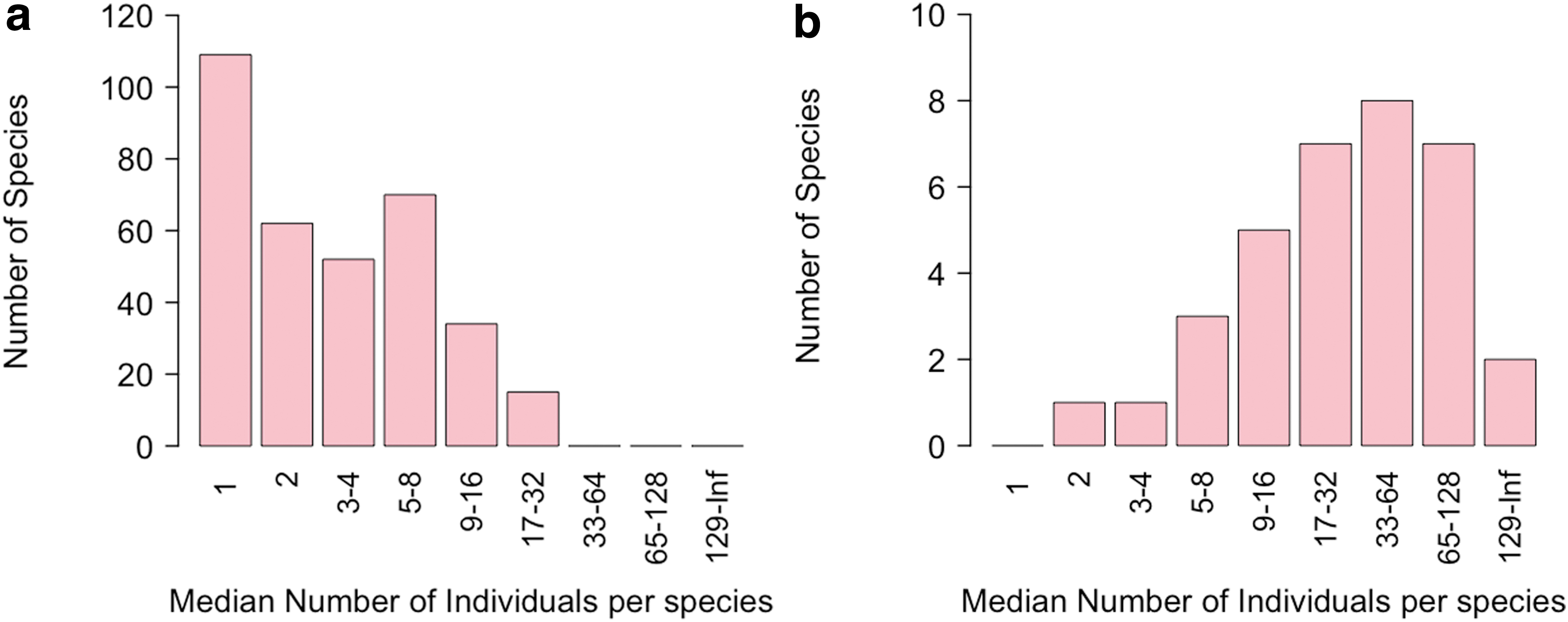
Presentation and comparison of the individuals' distribution in abundance octaves according to Preston for
The first plot (Fig. 2a) that represents the individuals' abundance per species for the initial species richness (342 species) has a great number of species that have only one individual. The plot is clearly positively skewed (∼0.46) with a large number of species with only one or two individuals.
The second plot (Fig. 2b) depicts the median number of individuals per species for the last 34 (10%) species retained. The plot presents a small positive skewness (0.22), which means that the data are more symmetrically distributed than in the previous case. In addition, there are more species with relatively large and viable populations, rather than those with only one to two individuals. In this study, we observe that the most abundant octave's height is quite close to the neighboring ones, a fact that renders the plot more symmetrical.
Another question arising at this point is whether the species diversity in these last stages of plant community development has stabilized and therefore only specific species are expected to survive or if there is any variance. When analyzing the 34 species composing the list of last 10% that remain, a brief change was observed for those found in the last ranks (i.e., less abundant species).
The results are presented in Supplementary Table S5, where a small oscillation is observed in the last six ranks (from the 28th most abundant species to the 34th). In the final two ranks, the variance becomes greater as three different species compete to remain. Nevertheless, it seems that the initially most abundant species have a head start and are expected to persist and establish over time.
By the end of the 2-year enclosure period of the first mission in Biosphere 2, as mentioned above in Section 1, only 744 of the initial 1571 individuals (a 52.6% loss) were left. These individuals belong to 205 different species (some species were not fully identified and only genera were recorded). The results are presented in Supplementary Fig. S3.
The results show that we expect an average of 259.6 (±6.123) species to remain. According to a t-test, this is significantly greater than the actual number remaining (p-value <2.2 × 10⁻¹⁶). This result further demonstrates that the species loss in Biosphere 2 was not random. Thus, the random loss of 52.6% of individuals does not explain such a large loss of species.
Discussion
In this work, we have tried to predict how communities should evolve if zero-sum dynamics based on the neutral biodiversity theory prevail and to compare our results with the actual experimental outcomes, such as those of the plant biome in Biosphere 2.
Our first goal was to assess what would be the expected evolution and succession pattern in a community under neutral dynamics. The output of our model indicates that when zero-sum dynamics are in force, the initial species loss is fast, with an important part of the biodiversity being lost in a relatively short time. As species richness decreases, however, the remaining species persist longer so that extinction of these could take many centuries. Especially after ∼90% of the initial richness is lost, the time to extinction increases enormously.
Competition to survive is present throughout the simulations. However, there is variance as to the identity of the last remaining species. This is not a surprise because in a neutral community, the winner is entirely dependent on luck since all species are equally “fit” in a neutral model. The least abundant species are left to compete for survival, whereas the most abundant species have already established their ranges. Randomness is the main driver of this phenomenon.
Another important issue concerns the species abundance distribution (SAD) of the initial and long-term simulated communities, for example, the community when only 10% of the initial species richness remains. Initially, the SAD may have a long tail and many singleton species, as that for Biosphere 2. Later, however, the Preston plot shows a more bell-shaped distribution with medium-sized groups being the most abundant ones.
This is in line with ecological intuition since in the long term, each species must have enough individuals to be viable to survive. The initial dynamics reflect a loss of species too rare to be viable and a consolidation of species that are already abundant. The asymmetric, long-tailed initial distribution is not that of a viable isolated community. Once this sample becomes a community itself, it means that there must be a consolidation of the core species in the new community with fewer species on the threshold of extirpation.
Biosphere 2 had some issues at the end of the first 2-year enclosure, which had not been expected. The plant biodiversity of the tropical rainforest area lost 40% of its initial known species. This correlates with the expectation of species loss in a neutral community, but it is much greater than what is expected. To some extent, this difference might be blamed on the fact that our choice of generation time of 18.5 years is very long and that many of the plants in Biosphere 2's initial rainforest community were annuals or biennials.
Suppose we go with this criticism and instead choose a half lifetime of τ = 1/2, as if all plants were annuals, this would reduce t 50 by a factor of 2 × 18.5 = 37, leading to a new t 50 = 409/37 ≈ 11 years. With such a half-life, we would expect [using Eq. (1)] a more substantial loss of about 15.3% after 2 years, but this is still much smaller than the observed 40% loss.
Another important factor was the loss of actual plant population, which fell from 1571 to 744 individuals. This loss was extremely fast and these individuals lost were not replaced by new births (Leigh et al., 1999). A possible explanation for this loss of individuals is Yoda's self-thinning rule (Mrad et al., 2020; Westoby, 1984). According to this theory, plant loss can be described as a result of plant competition due to increasing density and biomass.
Mortality is initiated as plants grow in size and their energy requirements become greater, exceeding the area's carrying capacity. The rate and speed of mortality also depend on the growth conditions, which in the case of Biosphere 2 were designed to be optimum. This usually entails a loss of biodiversity, but our simulations suggested that the loss of species in this process is only expected to be about 22 species, only a 7.8% loss.
Thus, the loss of biodiversity over the 2 years of operation of Biosphere 2 cannot be explained either by neutral dynamics or by self-thinning. Instead, there are other issues that must be considered to explain the large loss of biodiversity in Biosphere 2.
Biosphere 2 seems to have been the most extended and large-scale closed ecosystem experiment conducted to date, and it is also unique in its attempt to support autonomous closed ecosystems. However, it faced a series of problems that damaged the ecosystems and put the lives of the Biospherians in danger and so was closed down prematurely. The scarcity of data from other closed ecosystems of this caliber renders the explanation of its results difficult and uncertain.
The NTB helps explain how the experiment might have gone in the absence of the specific problems that arose, but only under the influence of zero-sum dynamics. For example, in a neutral community the size of the Biosphere 2 tropical plant biome, the length of time it takes half of the species of an autonomous isolated ecological community to go extinct due to random demographic processes should be 409 years (or 11 years if all are annuals).
This biodiversity half-life provides a measure of the time horizon we need to assess whether the population dynamics of the ecological community are working as they should be. For example, it has been argued that Biosphere 2, in subsequent experiments, “reached stability.” To assess the credibility of such claims, an experiment of such size (at least the “ecological community” part of it) needs to be allowed to run for at least the time previously mentioned.
There were no previous or subsequent experiments of similar size and scope as Biosphere 2. Nevertheless, there have been many attempts to realize isolated microcosms in extreme environments. The BIOS-3 experiment that was conducted in Siberia, earlier than Biosphere 2, had been evolving and improving based on information from previous experiments (BIOS 1 and 2). The final setup consisted of four chambers, one for human survival and the other three for crop production; this could host missions of three humans.
Three missions were conducted in total, and in each case, the system was able to sustain humans who suffered minor problems during the enclosure (Salisbury et al., 1997). The CEBAS closed aquatic system, set in a 9-day spaceflight, gave positive results for survival in space. The experiment was conducted without the presence of humans. The minimodule consisted of four compartments that were linked in the mode of a simple closed loop.
By the end of the experiment, the results were promising and similar to the ones conducted on Earth, where a second identical experiment had been simultaneously run (Bluem et al., 2000). More recently, the Lunar Palace 1 experiment had been simulating the conditions of a Moon base. The facility consists of a 160-m2 area and has operated in two different missions that lasted a total of 105 and 370 days (Fu et al., 2016, 2021).
The experiments described above not only had no recorded loss of individual species but also their duration and species abundance were shorter than those of Biosphere 2. After consulting the relevant literature regarding the duration and number of species in each experiment, we created the conceptual diagram presented in Fig. 3, which assesses the mission time as a function of the size of the ecological community.
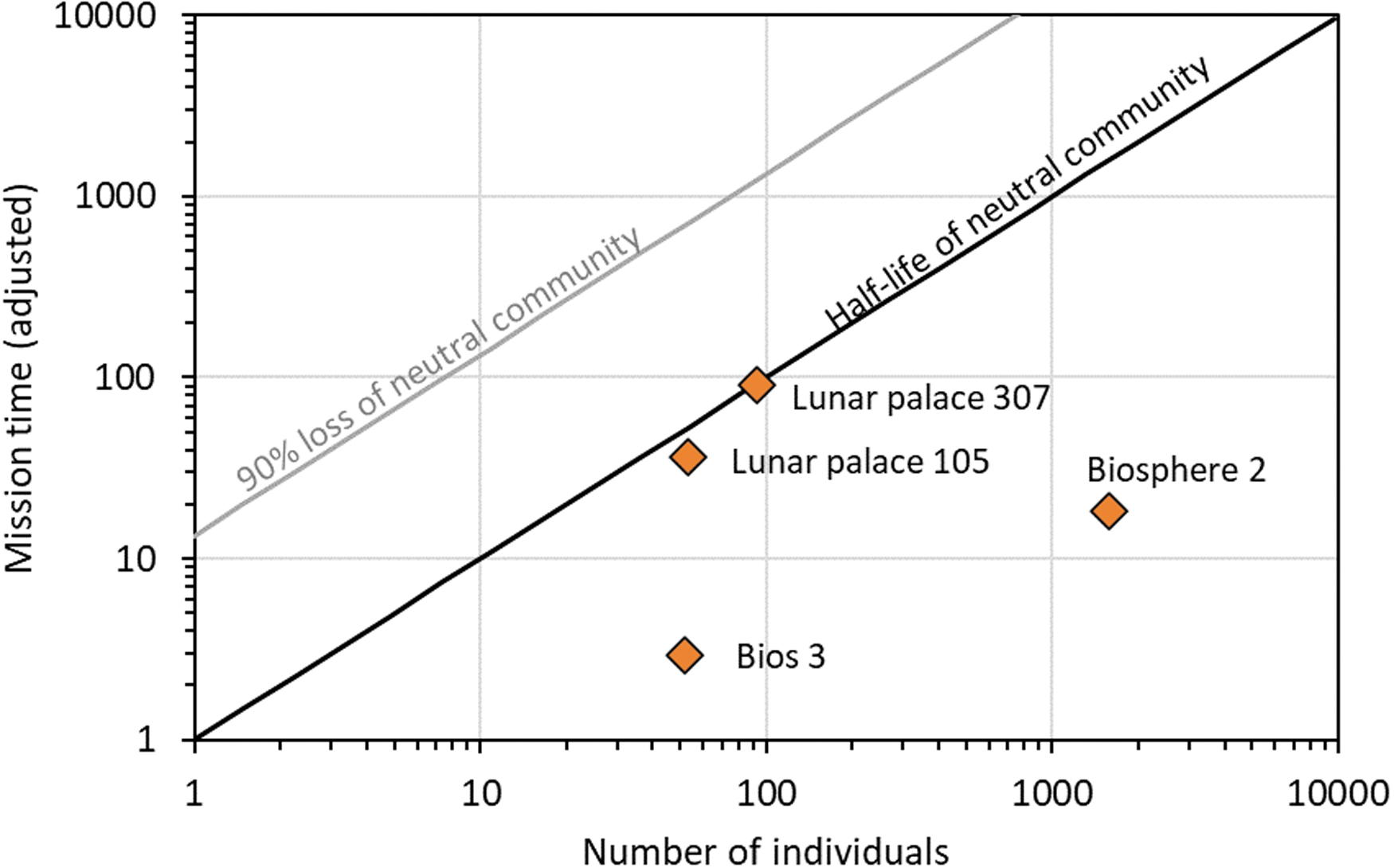
Comparison of different systems used to study systems of extreme isolation with the loci for the half-life of a neutral community and the time to 90% loss. In each case, the mission time was adjusted by the factor of (S 0/τ). For Biosphere 2, only the tropical rainforest region data were used (see Supplementary Table S6). Color graphics are available online.
In future space applications, if the mission time Δt is significantly greater than the biodiversity half-life, then a significant loss of species will begin to occur. Typically, the higher the number of individuals in the onboard ecosystem (for a given diversity), the longer the half-life (following Equation 2). We can define an adjusted mission time as Δt′ = (S 0/τ)Δt.
If we apply the same adjustment to half lifetime, we see that t 50 ′ = N, which is the adjusted time it takes a system to lose a significant portion of its biodiversity due to random drift. Figure 3, thus, compares the time required for loss of 50% of the species through neutral drift with the operating times of various systems.
In general, systems have not operated long enough to encounter the problem of biodiversity loss. This is especially true for Biosphere 2. It is therefore clear that realistic tests for systems of extreme isolation will need to run for longer to be fully credible.
As the knowledge of what lies beyond our planet grows day by day (Serjeant et al., 2020), the prospects of manned space exploration missions are more prominent than ever. An understanding of the intrinsic interactions that rule our own planet should be a major goal for preservation of life both on Earth and in other isolated systems. Biosphere 2 has been the longest-running experiment carried out in full isolation (Mohanty et al., 2008).
Due to the huge diversity of factors encapsulated in Biosphere 2, it has been the object of studies focusing on different aspects (Finn et al., 1999; Cockell et al., 2000; Nelson et al., 2015). At the same time, closed ecosystem designing and the ecological interaction issues arising generally from such enclosures have also preoccupied researchers (Cohen and Tilman, 1996; Bolger, 2001; Petersen and Hastings, 2001; Petersen and Englund, 2005).
In this study, we have gained valuable new insights into the evolution of the tropical rainforest biome of Biosphere 2 and its plants using the NTB to understand and analyze the process of plant succession and their interactions. Within the context of the neutral theory, we have considered various approaches concerning the evolution of the plant community.
The possible succession stages and expected lifetimes of tropical rainforest region plants were studied under the hypothesis that neutral equilibrium was the dominant mechanism. Thus, the NTB provides a new and useful insight into the way we interpret the evolution of Biosphere 2 and can offer an important perspective to the study of microcosms in general.
Footnotes
Acknowledgments
The authors thank Dr. Martha Charitonidou (Laboratory of Ecology, University of Ioannina) for input and valuable discussions about this work; Professor Uffe Gråe Jørgensen (Niels Bohr Institute, University of Copenhagen) for support and suggestions; and the members of our sections for the ideas and contributions.
Authors' Contributions
E.S. was involved in conceptualization, methodology, investigation, formal analysis, and writing—original draft. J.M.H. was involved in conceptualization, validation, writing—review and editing, visualization, and supervision.
Author Disclosure Statement
No competing financial interests exist.
Funding Information
E.S. was financed by the Novo Nordisk Foundation Interdisciplinary Synergy Programme, grant no. NNF19OC0057374.
Supplementary Material
Supplementary Figure S1
Supplementary Figure S2
Supplementary Figure S3
Supplementary Table S1
Supplementary Table S2
Supplementary Table S3
Supplementary Table S4
Supplementary Table S5
Supplementary Table S6
Abbreviations Used
Associate Editor: Radu Popa
References
Supplementary Material
Please find the following supplemental material available below.
For Open Access articles published under a Creative Commons License, all supplemental material carries the same license as the article it is associated with.
For non-Open Access articles published, all supplemental material carries a non-exclusive license, and permission requests for re-use of supplemental material or any part of supplemental material shall be sent directly to the copyright owner as specified in the copyright notice associated with the article.
