
Abstract
In Lammer et al. (2024), we defined Earth-like habitats (EHs) as rocky exoplanets within the habitable zone of complex life (HZCL) on which Earth-like N2-O2-dominated atmospheres with minor amounts of CO2 can exist, and derived a formulation for estimating the maximum number of EHs in the galaxy given realistic probabilistic requirements that have to be met for an EH to evolve. In this study, we apply this formulation to the galactic disk by considering only requirements that are already scientifically quantifiable. By implementing literature models for star formation rate, initial mass function, and the mass distribution of the Milky Way, we calculate the spatial distribution of disk stars as functions of stellar mass and birth age. For the stellar part of our formulation, we apply existing models for the galactic habitable zone and evaluate the thermal stability of nitrogen-dominated atmospheres with different CO2 mixing ratios inside the HZCL by implementing the newest stellar evolution and upper atmosphere models. For the planetary part, we include the frequency of rocky exoplanets, the availability of surface water and subaerial land, and the potential requirement of hosting a large moon by evaluating their importance and implementing these criteria from minima to maxima values as found in the scientific literature. We also discuss further factors that are not yet scientifically quantifiable but may be requirements for EHs to evolve. Based on such an approach, we find that EHs are relatively rare by obtaining plausible maximum numbers of
Introduction
Whether we are alone in the Universe or life might be common within the Milky Way and beyond is a fundamental question that has occupied mankind for centuries. As Giordano Bruno puts it in his famous work “De l’infinito universo et mondi” (Bruno, 1584):
In space there are countless constellations, suns, and planets; we see only the suns because they give light; the planets remain invisible, for they are small and dark. There are also numberless earths circling around their suns, no worse and no less than this globe of ours. For no reasonable mind can assume that heavenly bodies that may be far more magnificent than ours would not bear upon them creatures similar or even superior to those upon our human Earth.
More than 500 years later, astronomers were by now able to discover well over 5000 of the once-invisible planets. Whether at least some of these heavenly bodies are indeed similar to Earth, and bear any kind of living creatures upon them, however, remains unknown until this day.1
Even more so, as already pointed out within part one of our study (Lammer et al., 2024, thereafter called Paper I), not even a clear and unambiguous definition of the expression “Earth-like” can be found within the scientific literature. The related term “Eta-Earth” (
Within Paper I, we define the term EH as a rocky exoplanet within the HZCL, that is, the HZ of complex life3 (Schwieterman et al., 2019a; Ramirez, 2020, see also Sections 5.2.1 and 6.1.1) that evolved an N2-O2-dominated atmosphere with minor amounts of CO2 as a result of geologic activity and the emergence and evolution of (microbial) life.4 Such an Earth-like atmosphere would most likely constitute a geo- and biosignature (see Paper I, Stüeken et al., 2016; Lammer et al., 2019; Sproß et al., 2021) since this particular combination of atmospheric gases would not be stable over geologic timescales without working carbon–silicate and nitrogen cycles, and without the prevalence of microbial life that can recycle fixed nitrogen back into the atmosphere. Such an atmosphere also presents a biogenic disequilibrium (Krissansen-Totton et al., 2018), and hence again, a remotely detectable biosignature.
Even if it turns out that abiotic pathways can lead to N2-O2-dominated atmospheres, it will nevertheless constitute an EH as these conditions are crucial for most of present-day life on our planet. Finding such a world would therefore, in any case, signify an immense milestone toward better understanding the prevalence of life in the Universe.
Because the term
While Paper I presented our hypothesis and formula to calculate such a maximum number, the present work will apply this equation by including our current knowledge about stellar evolution, galactic habitable environments, and the evolution and stability of EHs. Since the present status of research can only quantify some of the relevant parameters, while others remain poorly constrained, and therefore neglected within our estimate, our calculation can only provide a maximum number of EHs. This result, however, will be further refinable in the future when observatories such as the James Webb Space Telescope (JWST) and Extremely Large Telescope (ELT), and potentially Large Interferometer for Exoplanets (LIFE) and Habitable Worlds Observatory (HWO) provide us with spectroscopic data of rocky exoplanet atmospheres within the HZs of their host stars. While earlier approaches to estimate habitable worlds or even intelligent life in the galaxy such as those based on the Drake equation (Drake, 1965; Vakoch et al., 2015) and/or on
In the next section, we briefly summarize our formula for deriving the maximum number of EHs,
A Formula for Estimating the Maximum Number of EHs
A famous way to estimate the number of communicating extraterrestrial civilizations in the Milky Way was proposed by Frank Drake in the 1960s (Drake, 1965), that is,
Our approach to estimating the maximum number of EHs does not take into account
As outlined in Paper I, our basic equation to derive
The parameters
The second term,
Finally, the term
Here,
Several other factors that may be subsumed within
The second term in Equation 4,
Another factor feeding into
The final term within Equation 4 constitutes
Volcanic degassing might not be able to resupply enough N2 if no tectonic processes exist that provide the right parameter range for oxygen fugacity, pressure, and temperature within the mantle to convert NH3 and NH
So, the origin of life,
We discuss most of the requirements above in more detail within Sections 5, 6, and Appendix 5. Next, we outline our general model approach and discuss related methodological issues, for example, the potential positive or negative correlation between different requirements.
Outline and model approach
The main aim of our study is to apply our formula, as derived in Paper I, for estimating the maximum number of EHs in the galaxy. By now, several studies calculated the number of HZ rocky exoplanets within the Milky Way (Bryson et al., 2021) or estimated the amount of communicating extraterrestrial intelligences (CETIs) that may presently exist in the galaxy (Westby and Conselice, 2020). However, no study to date has applied the current knowledge about scientifically quantifiable stellar or planetary requirements that are needed for EHs to evolve onto the distribution of presently existing stars and planets within the Milky Way to derive a maximum number of EHs, on which life as we know it might indeed be able to originate and evolve.
To do so, we first calculate the distribution of stars,
All the galactic, stellar, and planetary requirements that need to be met for EHs to evolve will be applied to the distribution of stars within the galactic disk. This will finally give us the distribution of EHs as functions of galactic spatial location, stellar mass, and stellar birth age. Crucially, the received numbers will be plausible maximum numbers since several necessary and potentially necessary requirements are not implemented in our model. These criteria are evaluated further in the appended Section 5. Our results are finally summarized and discussed within Section 7.
For deriving our EH distribution and maximum numbers, we perform 6 different model runs for which a summary of all input parameters, including their scientific sources, can be found in Section 8. First, we calculate our distribution for two types of atmospheres, that is, for N2-O2-dominated atmospheres that have a maximum mixing ratio of 10% CO2 (i.e., for N2-O2-dominated atmospheres that have a maximum mixing ratio of just 1% CO2 (i.e.,
In addition, we perform three different model runs for the two atmospheric cases, that is, a nominal case, which always implements mean values for the input parameters from the scientific literature—this often coincides with the values assumed to be most realistic and/or reliable by the published studies we investigated; a maximum case, for which we always implement reasonable maximum values; and a minimum case that conversely takes into account minimum values.
Combining our two atmosphere scenarios with nominal, maximum, and minimum cases results in the aforementioned total of 6 different model cases. Atmospheric composition does not feed into our calculations before investigating the effects of stellar short-wavelength radiation; our model cases will therefore increase from 3 to 6 not before Section 5.2. We, however, from time to time discuss other potential scenarios in case there are alternative input parameters.
Within each section and their related appendices, we review the importance of the different requirements, discuss and estimate their occurrence rates, prescribe their implementation into our model cases, and present their effects on the sample of stars/planets in the galactic disk. For this, we start with the entire distribution of stars (Section 4) and then apply one necessary requirement at a time to the (remaining) distribution. With each implemented criterion, the sample of remaining stars/planets will therefore decrease until we receive our final maximum distribution of EHs in the galactic disk. At the end of Sections 4, 5, and 6, we present a Summary section where we discuss our derived results and distributions for
Caveats, methodological, and philosophical issues
This model approach comes with several caveats, as well as implicit and explicit assumptions. These can be divided into five broad categories as described in the following.
Uncertainties in the magnitude of the involved variables
Many factors that feed into the emergence and evolution of EHs cannot be scientifically quantified at present (see specifically Appendix 5), whereas others are only quantifiable up to a certain, low extent. Although our approach allows to set most of them equal to 1, several implemented parameters remain that are still highly uncertain. A prominent example is “Eta-Earth” itself, the occurrence rate of rocky exoplanets in the HZ of solar-like stars (see Sections 6.1.1 and B); an important variable through which we estimate the occurrence rate of rocky exoplanets in the HZCL. Literature values for
However, further difficulties come into play here. The most crucial one relates to the fact that no rocky exoplanets were yet discovered in the HZ of solar-like stars, implying that observations from either lower mass stars or tighter orbital periods must be extrapolated. This is nontrivial since additional effects such as dependencies with stellar mass or temperature must be accounted for. Another often neglected effect that is increasingly taken into account in recent years relates to atmospheric erosion of primordial atmospheres on close-in orbits (Neil and Rogers, 2020; Pascucci et al., 2019), an important process that can lead to substantial overestimates of
Scaling from a specific range of orbital periods and radii to different parameter ranges, or from a specific stellar mass to another, as we need to perform for deriving the occurrence rate of rocky exoplanets in the HZCL, brings in further uncertainties, although these will be less pronounced than the inherent uncertainties in Eta-Earth itself. However, it will take quite some time until new instrumentation will discover rocky exoplanets in the HZs of solar-like stars and it will even take longer until robust occurrence rate statistics will exist on
Certainly, Eta-Earth is not the only parameter with high uncertainties. While the stellar parameters in our model are comparably well defined, any planetary parameters must be taken with caution. This is also true for the occurrence rate of planets with an appropriate water mass fraction and the frequency of large moons as both are mostly based on theoretical models but not on direct observations.8 Also, atmosphere and GHZ models are mostly based on theoretical considerations and on inherent assumptions that can lead to high uncertainties. As an example, are all relevant cooling agents implemented in an atmospheric model or are important molecules omitted, forgotten, or even unknown that may lead to a change in thermal stability (Section A)? What actually quantifies as a SN “sterilization” event is another relevant example.
These uncertainties are one of the reasons why we include literature reviews on various related topics (as mostly found in the appendices) and implement each of the parameters from comprehensive literature-based minimum to maximum values. They also highlight the possibility that our estimates can significantly change in the future when new models and observations are available.
Uncertainties in the choice of requirements themselves
Our derived formulation relies on the implementation of clusters of necessary requirements. However, whether a “necessary requirement” is indeed a necessary requirement is a category of caveat in itself (Ćirković, 2012). Although some of them are well accepted, others are not. The existence of a host star around which the rocky exoplanet orbits in the HZ is certainly well accepted, at least for the type of habitat we are considering, that is, for an “EH.” We define this as a rocky exoplanet within the habitable zone of complex life (HZCL) on which Earth-like N2-O2-dominated atmospheres with minor amounts of CO2 can exist. Although this sounds almost tautological, this is not necessarily the case for other potential habitats such as the recently suggested Hycean worlds (Madhusudhan et al., 2021) for which no host star would be needed,9 for subsurface ocean worlds (Nimmo and Pappalardo, 2016) and planets with deep biospheres (Lingam and Loeb, 2020; McMahon et al., 2013), both of which do not have to orbit in the HZCL at all, or for brown dwarf (BD) habitats, which neither need a host star nor a conventional HZ, a rocky surface or an N2-dominated atmosphere (Lingam and Loeb, 2019a). It is, however, less simple for other requirements.
Another example relates to the “right amount of water,”
There is another type of category, that is, the ones that are strongly debated and may finally not turn out to be a requirement at all. Most of them we did not implement into our model (some of these are discussed in Appendix 5), but one specific example we did, that is, the potential requirement of possessing a large moon. The initial argument in favor of the “Rare Moon” relates to the need for a large satellite to stabilize obliquity variations (Laskar et al., 1993). As it turned out, such an argument was not confirmed by simulations afterward (Waltham, 2019a), thereby illustrating that specific arguments must not necessarily be true. However, even though several further arguments in favor of a large moon exist (see appended Section 4.1), one could apply a similar reasoning as discussed above related to the water issue. Although we implemented a relatively “optimistic” parameter range for the occurrence rate of large moons (see Sections 6.3.1 and D.2), it may still overestimate its relevance if the requirement turns out to be negligible. On the contrary, if its importance will be confirmed in the future and if large moons are indeed rare, then our implemented parameter range could be too optimistic. Future observations can give important hints on this issue and on the uncertainties in the various parameters in general.
Methodological issues
Our formulation closely relates to the famous Drake equation (Drake, 1965) and therefore inherits some of its difficulties to a certain extent. One crucial problem with this type of equation is its lack of temporal structure (Ćirković, 2004; Lingam and Loeb, 2021). In its usual version, the Drake equation assumes a uniformity in time. As an example, the SFR of the galaxy feeds into the Drake equation via
A similar assumption could be introduced for the GHZ by assuming that the Milky Way may have been uninhabitable in the past due to frequent SNs, again suggesting a stepwise function of habitability. In this case,
However, our approach is not entirely equivalent to a uniform, step-less Drake equation since we effectively try to tackle this problem for specific parameters. As described in the following sections, we indeed implement the SFR, IMF, and stellar main-sequence lifetime into our model to arrive at a stellar age distribution for the Milky Way. This is of fundamental importance due to the aforementioned metallicity evolution and the thermal stability of N2-dominated atmospheres. Because of the latter, we must account for stellar evolution, otherwise we could not calculate which stars allow for such atmospheres to be thermally stable (which is roughly favored for older stars; see appended Section 1). In the same manner, we also implement the evolution of galactic metallicity for considering the temporal distribution of rocky exoplanets. If we neglected these evolutionary parameters, we would overestimate the number of stars that can in principle host Earth-like atmospheres.
We do, however, not consider the evolution of SN rates, which indeed introduces a methodological uncertainty due to the spatial dynamics in the galactic disk. Drake equation-like formalisms cannot properly account for such dynamics, which is also true for our present framework. As an example, even though we only need to know the probability distribution of being sterilized by SNs for the present day, this does not assure us to choose the correct stellar systems for being sterilized because of neglecting stellar migration within the disk. A hypothetical star could, for example, migrate from a denser, more metal-rich region in the inner disk outward toward a metal-poorer region with far less detrimental SNs. This star could therefore have a sufficient metallicity for forming planets without being sterilized by SNs exactly because of its migration toward a quieter region. Since we ignore such migration, however, the same hypothetical star could have ended up being sterilized as it would have been if it had remained in the inner disk.
There are further evolutionary aspects we do not currently consider in our framework. One important example relates to the evolution of planetary atmospheres. Their composition (and pressure) can significantly change over geological timescales, thereby strongly affecting their thermal stability against atmospheric escape into space (see Sections 5.2.1 and A.2). Conceptually this is a crucial point in our formulation, although we do not consider it explicitly (but assume it implicitly). After the active phase of a star, when an N2-dominated atmosphere theoretically becomes thermally stable at a planet, it must not necessarily be the case that such atmosphere will indeed evolve. We presently assume that any planet around a sufficiently weakly active star will host such an atmosphere—certainly a clear overestimate (see appended Section 5.2.1). We therefore set this requirement equal to unity, as we do with all requirements that are not implemented into our model.
Another crucial limitation of a Drake equation-like approach is the simple multiplication of parameters that may or may not be independent of each other (Ćirković, 2012). In reality, some of the parameters feeding into Relations 2, 3, and 4 can be positively or negatively correlated, implying that the outcome could be either an overestimate or underestimate, if known correlations are not addressed properly. We give some examples in Paper I, but here we emphasize an obvious positive correlation between two well accepted necessary requirements that we did indeed implement. These are the stellar metallicity and the occurrence rate,
Potential correlations could in principle be tested and explored by performing statistical tests. This also includes the implementation of probability distribution functions instead of mostly taking point values or ranges (although these variables vary over space, time, and stellar mass in our model). This was already pointed out by several different authors who highlighted point variables instead of probability distribution functions to be another major limitation of the classical Drake equation (Glade et al., 2012; Lingam and Loeb, 2021; Maccone, 2010, 2011). However, implementing probability distribution functions is beyond the scope of the present study.
This brings us to a final methodological issue. As written above, we run three different cases for two types of atmospheres, a nominal case for which we always take mean values from the scientific literature, and minimum and maximum cases for which we always take minimum and maximum values, respectively. Therefore, both minimum and maximum cases are statistically highly unlikely since it is improbable that any chosen parameter will always reach either its theoretical minimum or maximum in reality. Based only on the implemented requirements, this would necessarily imply that the minimum cases are too low and the maximum cases are too high, with the actual values being closer toward the nominal cases. We further emphasize that this methodology still only results in a variation of the maximum number because several necessary requirements are not implemented into our framework but simply set equal to unity. Given this, it makes sense to not only consider maximum values for calculating the actual maximum number of EHs within the galaxy but to use the entire value range of each parameter from minimum to maximum for illustrating the uncertainties within the present scientific knowledge as well. If we were to only calculate the maximum number of EHs with strict maximum values from the scientific literature, the results would (i) pretend a strict theoretical maximum by neglecting any uncertainty range, and (ii) give unrealistically high maximum numbers as just described above.
Neglected factors
As already mentioned above, our approach ignores any potential requirements whose occurrence rates cannot be properly assessed with our current scientific knowledge. The occurrence rate of all these requirements is set equal to 1, which implies that our derived number of EHs must represent a maximum number by definition. The actual occurrence rate of EHs should therefore always be lower than the rate found by our formulation. An extensive list of potential galactic, stellar, planetary, and biological requirements ignored by our present study can be found in Appendix 5.
Our present formulation is further restricted in terms of potential habitats that it can presently cover, as it is designed for investigating the occurrence rate of EHs. It therefore does not cover any other hypothetical habitats such as subsurface ocean worlds, or more exotic ones such as the aforementioned Hycean worlds. However, this restriction is again by design. We are specifically interested in EHs because we can evaluate their existence at least partially based on some hard physical parameters. The most crucial of these parameters is the thermal stability of Earth-like atmospheres, that is, N2-O2-dominated atmospheres with a minor amount of CO2. In this study, we emphasize the specific importance of the minor species CO2, which not only relates to atmospheric stability but also to the toxicity limits of complex life (see below). Based on such relatively well understood atmospheric parameters, we can show that by far, not all stars are able to presently host EHs. This is a crucial point to emphasize because, based on specific known requirements, our formulation allows to derive some information on the prevalence of EHs. Even though this may seem similar to an anthropocentric ansatz, it is less clear how we can retrieve similar information on other types of habitats as our knowledge about them is much more restricted.
Another advantage of our approach relates to observability. Even though we are presently not at a stage where we can directly observe N2-dominated atmospheres, we will be able to do so in the future. In the meantime, we can already start doing atmospheric statistics that will give important insights into the prevalence of EHs: If most planets in the HZCL have H2- and/or CO2-dominated atmospheres or even none at all, we can induce that N2-dominated atmospheres will likely be rare. One can also infer that finding an N2-O2-dominated atmosphere will likely be an indication for life since these atmospheres function as a biosignature (see Paper I). This is an exciting prospect that makes deriving the maximum number of EHs in unison with their stellar/galactic distribution a worthwhile study to endeavor.
We should further explicitly highlight that we do not exclude the actual existence of other forms of habitats. If EHs are rare compared with the number of stars, it may well be that other forms of habitats could be more abundant. Although we are at present simply agnostic about them, we discuss a pathway for extending our formalism toward other forms of habitats in Section 7.8. We also point out that our formulation does not cover CETI like the Drake equation does. Also for this, we suggest a potential extension in Section 7.9.
Finally, we only investigate the galactic disk and neither the galactic bulge nor the galactic halo (as detailed in Section 4.1). We further neglect any space beyond our galaxy as it is not entirely trivial to expand our formalism toward a broader region of the Universe (Gonzalez, 2005). In addition, we neither calculate the evolution of habitability nor the maximum number of EHs throughout galactic history. Our calculations only relate to the present day. Finally, we want to emphasize that we do not consider parameters that may increase the maximum number of EHs. Obvious examples could be panspermia or the existence of hypothetically habitable exomoons. We do, however, discuss these issues in some detail in Section 7 and Appendix 5.
Some philosophical issues
As a last category, we briefly discuss certain philosophical issues related to our methodology, of which the definition of complex aerobic life is the most critical. We already discuss this issue in detail in Paper I and therefore keep it relatively short but it is of importance to reiterate it here. Our definition closely follows three studies that discuss certain atmospheric toxicity limits for complex life. These are Catling et al. (2005) related to O2, Schwieterman et al. (2019a) related to CO2, and Ramirez (2020) related to CO2 and N2, that is, the three prime atmospheric species for our framework.
Based on these studies, we use the terms “complex (aerobic) life,” “life as we know it,” “advanced metazoans,” and “animal life” synonymously to mean millimeter- to meter-sized carbon-based heterotrophs that are mobile and contain a blood-circulatory-like system comparable with advanced metazoans.10 Whenever we mean other forms of life in our study, we spell it out explicitly. We also note that focusing on habitats suitable to animal-like complex life, although it may seem arbitrary at first glance, may actually be well justified. On Earth, animals are the only complex multicellular eukaryotes capable of phagocytosis and animals are effective “ecosystem engineers.” For these reasons, Lingam and Loeb (2021) suggest that the evolution of animal multicellularity is one of the five, potentially universal, key critical steps for the emergence of technological intelligence on Earth and on exoplanets in general.11
Catling et al. (2005) precisely outline the universal importance of atmospheric O2 for such complex life by showing that a certain O2 partial pressure of pO
In this study, we need to highlight, however, that extraterrestrial life must not necessarily evolve toward similar toxicity limits but may find additional pathways to cope with toxic atmospheres, especially if the evolutionary pressure of survival is high. We nevertheless find these pressure limits to be a useful starting point for evaluating the prevalence of EHs in the galaxy even if such limits may vary substantially on other worlds. Until no other biospheres are found and investigated, it is reasonable to evaluate atmospheres within aforementioned limits as long as it is made clear that these can be substantially different for extraterrestrial complex life.
Whenever we talk about Earth-like atmospheres, we implicitly mean N2-dominated atmospheres with O2 as a second, less abundant main species, and with a minor amount of CO2. Such atmospheres can certainly include other trace species and the exact ratios of the three main species are not fixed as long as the CO2 mixing ratio is either below
This specific definition of an atmosphere also relates to our definition of what an EH actually constitutes. As we have already stated, we define an EH as a rocky exoplanet within the HZCL on which Earth-like N2-O2-dominated atmospheres with minor amounts of CO2 can exist. This definition in principle allows for the possible existence of complex aerobic life that obeys to similar limits as advanced metazoans here on Earth, but it is important to note that such putative organisms do not have to actually live on such a planet. However, the proposition that the Earth-like atmospheres themselves, that is, the simultaneous existence of N2 and O2 with minor amounts of CO2, act as a biosignature makes EHs extremely relevant for astrobiology in itself, regardless of whether complex life actually exists there or not.
Although EHs are close to the definition of Class I habitats in Lammer et al. (2009),12 both are not entirely the same since the latter does not directly relate to atmospheric composition. It does, however, relate to certain stellar and geophysical conditions needed for such habitats to evolve, which can be regarded to be semantically equivalent with our meaning of necessary requirement. Class I habitats further exclude ocean worlds explicitly on which the ocean is not in direct contact with the mantle silicates due to the formation of a high-pressure (HP) ice layer between both (such planets are defined as Class IV habitats in Lammer et al., 2009). We also exclude them from our definition, but this does not relate to ocean planets without subaerial land on which an HP ice layer may not exist. We discuss arguments on whether these planets could constitute an EH in detail in appended Section 3.1. However, we also note that Lammer (2013) refined the definition of Class I habitats, so that (i) it does exclude ocean worlds without subaerial land entirely (with ocean worlds constituting Class V habitats) and (ii) N2 as main species should be present in their atmospheres.13
If one takes the definition of EHs (or Class I habitats), it seems logical that it becomes narrower the more is scientifically known about said certain stellar and geophysical conditions. If we, for instance, could exclude planets without subaerial land based on future scientific knowledge, this will narrow down its definition and hence the number of planets that can evolve into an EH. One must, however, take care to not overspecify its definition, otherwise the definition of EH will be indistinguishable from Earth, and Earth will by definition be the only EH in existence. It is therefore important to keep a balance between a too narrow, tautological definition and a broader useful one that allows searching for planets on which complex aerobic life may evolve based on identifying and testing relevant and scientifically quantifiable requirements.
Another issue is related to the GHZ. It is important to highlight that the models we utilize for the sterilization rates of SNs were performed for complex life as defined above. As we discuss in Section 5.1, the effects of SNs would be less pronounced if we would only consider extremophiles or microbial life. We also want to mention that the definition of rocky exoplanet, and hence of “Earth-like” itself, seems to be slightly contentious, as there is no fixed mass or radius range that applies to the term rocky exoplanet. We discuss this in detail in Sections B and 6.1. Finally, we also emphasize that our results have certain philosophical implications such as for the Copernican Principle, the Fermi Paradox, and the Search for and Messaging to Extraterrestrial Life, that is, for SETI and METI. We discuss these potential implications in Section 7.
The Number of Stars Within the Milky Way
The components of the Milky Way and their relevance for estimating
The various components of the Milky Way
The Milky Way (see reviews by Bland-Hawthorn and Gerhard, 2016; Helmi, 2020) is a typical disk galaxy and can be divided into different regions, that is:
Galactic bulge
The galactic bulge is the high-density inner region of the Milky Way, which extends to about 2 kpc from the center (see Barbuy et al., 2018, for a recent review of the bulge and bar region) with an average stellar density of about 14 stars per cubic pc (Robin et al., 2003). Its structure is strongly barred with a long lower density bar extending outward from the bulge into the inner disk with a half-length of 5.0 ± 0.2 kpc (Wegg et al., 2015). The bulge itself holds a stellar mass of
Galactic halo
The halo (Belokurov et al., 2018; Helmi, 2020; Helmi et al., 2018) is the extended spherical part of the Milky Way and is populated by lone stars and globular clusters with metallicities that are mostly clearly below
Galactic disk
The galactic stellar disk (Bland-Hawthorn and Gerhard, 2016; Bovy et al., 2016; Helmi, 2020; Rix and Bovy, 2013) is commonly decomposed into two different components, for example, the thin and the thick disk (Gilmore and Reid, 1983). In this study, the thin disk is the main component of the Milky Way and the place of ongoing star formation with a current SFR of (Licquia and Newman, 2015). It has a compact scale height, a wide spread of different stellar ages and metallicities, and its origin (Kilic et al., 2017) can be traced back to about 8 billion years ago (Ga). The thick disk, on the contrary, has a larger scale height, but is much more diffuse than the thin disk (McMillan, 2017), and its age is of the order of 10 Gyr (Kilic et al., 2017). Its metallicity distribution function (MDF) peaks lower than for the thin disk at
In total, the Milky Way holds a stellar mass of about
For calculating
Excluding the galactic halo
As written above, the galactic halo mainly consists of metal-poor and old stars. Zuo et al. (2017), for example, can reproduce the MDF in the galactic halo well by separating it into three distinct groups with peak metallicities of (Fe/H) approximately −0.63, −1.45, and −2.0, where the two metal-poorer components correspond to the inner and outer halo, respectively.14 The additional, relatively metal-rich component, which corresponds to substructures within the galactic halo such as clouds, and streams such as the Sagittarius stream (Belokurov et al., 2007; Grillmair and Carlin, 2016; Koposov et al., 2012), covers about 10% of halo stars (Zuo et al., 2017). Similar results were found by other surveys, for example, (Fe/H) approximately −1.2 ± 0.3, and −2.0 ± 0.2 by Liu et al. (2018) for the inner and outer galactic halos, respectively.
It seems unlikely that many of them will provide habitable conditions at present, however. As already pointed out by Lineweaver et al. (2004), many of the halo stars will have metallicities that are too low to host rocky exoplanets, a threshold that might be somewhere around
In addition, the high majority of stars within the galactic halo, including the inner halo, are of an age of ∼10–12 Gyr (Jofré and Weiss, 2011) while the metal-rich stellar component of the Sagittarius stream holds ages of ∼9.5–11 Gyr (Carollo et al., 2016). Similar ages can be found for other metal-rich halo regions such as the Styx and Orphan streams, both of which were found to cover ages of ∼10–11 Gyr (Carollo et al., 2016). These stellar ages are significant, and one can expect that many of the rare planets that formed around these stars do not show geological activity at the present day, specifically if one considers that planets with an Earth-like radiogenic heat budget will be geologically active for about 6 Gyr (Mojzsis, 2021). These worlds would therefore provide relatively limited conditions for the evolution and maintenance of complex life. In fact, these stellar ages are even too old to generally allow inhabited planets around G-type stars based on their average main-sequence lifetime and bolometric luminosity evolution. EHs in the galactic halo must therefore logically be restricted either to old low-mass stars, which pose further difficulties (as discussed in later sections), or to one of the few younger ones that were either ejected out of the galactic disk (Faltová et al., 2023) or formed at younger ages under as of yet poorly constrained conditions (Bellazzini et al., 2019).
No study has explicitly modeled the habitability of the galactic halo, so no potential distribution can be incorporated within our model (as we do for the disk in the following subsections). However, even if there are stars within the halo that currently allow for the existence of an EH, their numbers will be minuscule, most likely significantly below 1 permille of the entire population, at least based on the considerations above. Due to their average distance, the potential to observe and characterize some of them in the near future may further be relatively elusive. Based on this reasoning, we therefore do not consider the galactic halo within this study.
Excluding the galactic bulge
The story looks a bit different for the galactic bulge. Depending on the specific study (Licquia and Newman, 2015; McMillan, 2017, 2011), its stellar mass amounts to about ∼20% of the entire galactic stellar mass. So, if we assume the bulge to be habitable, it cannot be neglected as long as we want to estimate the maximum number of EHs within the entire Milky Way. Whether the bulge is indeed habitable, however, is debated (Balbi et al., 2020), as outlined in the following.
The habitability of different galactic regions, which is often subsumed under the concept of the so-called GHZ, depends on various factors (Kaib, 2018) that are usually broadly divided into three (nonexhaustive) areas, that is, high-energetic events such as AGN, SNs, and GRBs that both sterilize a planet and erode its atmosphere; close stellar encounters that perturb the orbit of a planet and/or trigger comet and asteroid bombardments; and the metallicity of the local interstellar medium (ISM), which may hinder the accretion of rocky exoplanets around newly forming stars.
Several specific problems may arise for the bulge, particularly within (i) and (ii).
Since the stellar density in the bulge is significantly higher than in the disk and halo regions, it can be expected that a planet suffers from detrimental SNs more often than a planet in the other disk regions. As estimated by Gehrels et al. (2003), an SN within
Apart from SNs, GRBs (Gowanlock, 2016; Melott et al., 2004; Piran and Jimenez, 2014; Scalo and Wheeler, 2002; Thomas et al., 2021; Thomas et al., 2005b, 2005a) could be another threat within the bulge. Piran and Jimenez (2014), for example, found that these could render the galactic center inhospitable to life. However, a study by Gowanlock (2016) that considers the SFH and metallicity evolution of the galaxy suggests a more complex picture. If GRBs correlate with low-metallicity environments (Jimenez and Piran, 2013), predominantly the metal-poor outskirts of the Milky Way will presently be affected by GRBs. If GRBs, on the contrary, exclusively follow the galactic SFH, most of them will occur in the galactic center.
The supermassive black hole (SMBH) Sagittarius A
As a side note, it should be mentioned that the effect of the XUV flux from an SMBH on the atmospheric mass loss of a rocky exoplanet may be underestimated. Balbi and Tombesi (2017) and Balbi et al. (2020) calculate this process with the well-known energy-limited escape esquation (see Equation 25 in Section 6.2.1), in which the square of the photospheric radius,
Because of the high stellar density in the galactic center, stellar systems are susceptible to orbital perturbations by nearby stars (Balbi et al., 2020; Bojnordi Arbab and Rahvar, 2021; de Juan Ovelar et al., 2012; Jiménez-Torres et al., 2013; McTier et al., 2020). McTier et al. (2020), for example, found that 8 out of 10 bulge stars experience stellar encounters within 1000 AU at a rate of
Finally, we point out a potentially positive aspect of habitability related to the bulge. Apart from its generally high density of stars, which can be regarded as a positive aspect in itself at least related to the number of systems that can be examined per volume of space, the advantage for panspermia, that is, for transferring life from one stellar system to another, should particularly be highlighted (Adams and Spergel, 2005; Balbi et al., 2020; Belbruno et al., 2012; Chen et al., 2018; Gobat et al., 2021; Chen, 2021).17 In the bulge, the travel time of an ejecta for reaching the nearest star can be smaller by at least an order of magnitude compared with the galactic disk; it may hence be within the estimated survival time of certain extremophiles (Balbi et al., 2020; Ginsburg et al., 2018).
The arguments of the last paragraphs do not paint an entirely coherent picture or generally prove the complete noninhabitability of the galactic bulge, at least not for microbial life and/or extremophiles. However, they indicate that other galactic regions, particularly within the disk, might provide far more favorable habitable environments than the galactic center. Because of this and the lack of studies on the SFH and the distribution of SNs and metallicity within the bulge, we presently restrict ourselves to estimating the maximum number of EHs in the galactic disk.
To derive such a maximum number, however, we need to calculate the spatial distribution, age, and total number of presently existing stars in the galactic disk. To achieve such a distribution, we first need to implement the IMF and SFH into our model.
Implementing IMF, main-sequence lifetime, and SFH
The IMF
The IMF describes the initial distribution of stellar masses,
The lower stellar mass limit,
The Initial Distribution of Stars Within the Stellar Spectral Classes for Different Initial Mass Functions and
Mass range after (Habets and Heintze, 1981).
Salpeter (1955).
Miller and Scalo (1979).
Chabrier (2003).
The IMF was subsequently further investigated by several different authors (Chabrier, 2005, 2003; Kroupa et al., 1993, 2013; Kroupa, 2001; Miller and Scalo, 1979) to better fit the refined observational data. Kroupa et al. (2013) provide a thorough review of the IMF and propose a two-part power-law “canonical IMF” for masses between
By integrating this relation, we obtain the number of stars,
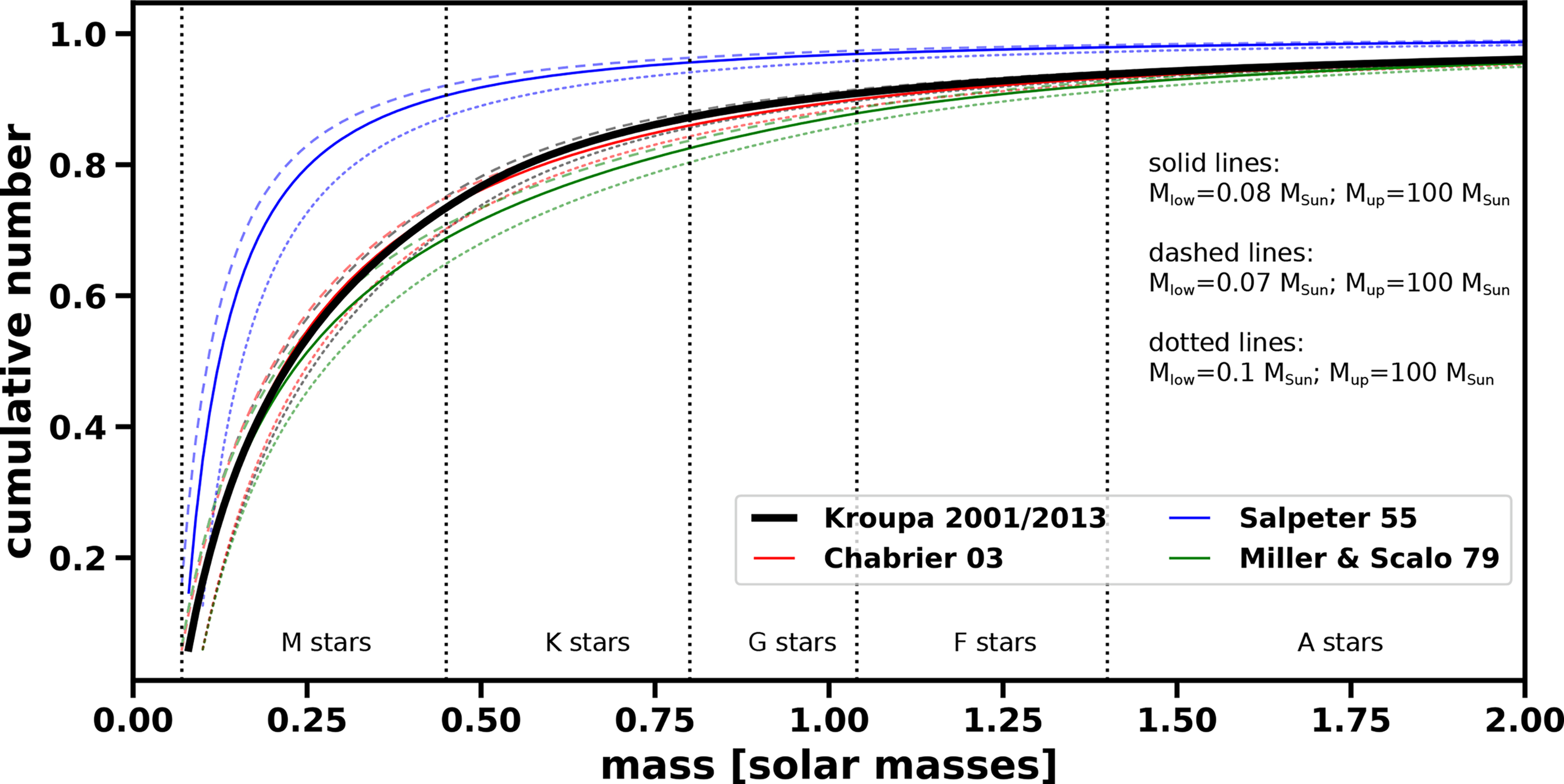
Different cumulative stellar mass distributions for different initial mass functions (IMFs), that is, of an initial population of stars, as calculated through the empirical power laws by Salpeter (1955), Miller and Scalo (1979), Kroupa (2001)/ Kroupa et al. (2013), and Chabrier (2003), displayed for stellar masses up to 2.0
We should finally mention that the IMF may not be constant but varies over time. Li et al. (2023), for instance, found that the relative fraction of low-mass M dwarfs that form during an episode of star formation increases with stellar metallicity and hence galactic age. Based on correction factors by Liu (2019) and Moe et al. (2019), Li et al. (2023) also provide an IMF correction for binary systems that may further increase the relative fraction of young low-mass stars. This indicates that a higher number of M dwarfs form at present than at earlier ages of the galaxy. Since we implement the canonical IMF and do not consider such variability, this may slightly affect our results. If we implemented a variable IMF instead, our stellar distribution would contain a higher number of young M dwarfs, while the fraction of stars in the other spectral classes would be slightly lower. Such alteration would potentially lead to a slightly lower maximum number of EHs since a larger number of stars would fail to meet
Since the IMF describes the initial stellar distribution, we need to implement the stellar main-sequence lifetime as a function of stellar mass to calculate the potential survival of a star until the present day. For the main-sequence lifetime, we follow the same approach as Westby and Conselice (2020) who combine the estimated main-sequence lifetime of the Sun of about 10 Gyr (Schröder and Smith, 2008) with the luminosity-mass correlation by Salaris and Cassisi (2005). This gives the following relationship between main-sequence lifetime,
By applying this relation, we obtain the black solid line in the upper panel of Figure 2, which illustrates the main-sequence lifetime of stars as a function of stellar mass. For comparison, the red line corresponds to a calculation performed with a similar relationship by Hansen and Kawaler (1994). The blue line additionally illustrates the “mean habitable lifetime for planets that may possess intelligent observers” by Waltham (2017) and was calculated with the power-law fit from the same study. Waltham (2017) based their mean habitable lifetime on a probabilistic combination of the Copernican and Anthropic principles and therefore assume planets to be inhabitable for intelligent life if these provide conditions similar to the Earth’s. Note, however, that (i) this lifetime is larger than the main-sequence lifetime for stars with masses below ∼0.6
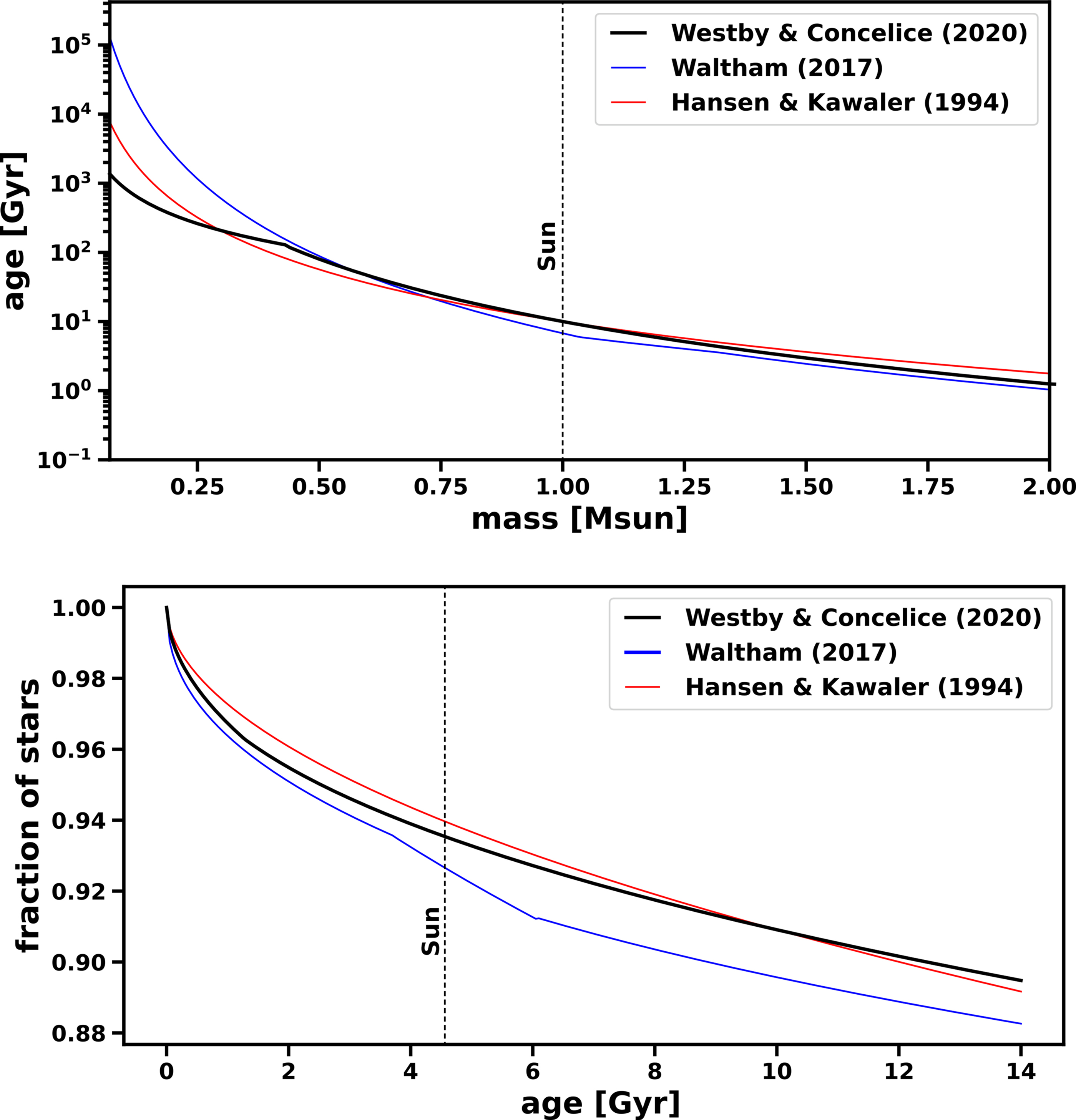
Upper panel: Main-sequence lifetime of stars with masses between 0.1M
While we implement the relationship by Westby and Conselice (2020) as an upper limit of stellar age into our nominal case (the white area in Fig. 4 derives from this limit), we see in Section 5.2 that our results are insensitive to the chosen stellar main-sequence lifetime relation. This is because the upper age limit of stars, which allow for the existence of EHs, will always be set by the maximum bolometric luminosity that still permits the survival of complex life in the HZCL, a value that will always be lower than the actual main-sequence lifetime (but may intersect with the mean habitable lifetime by Waltham, 2017).
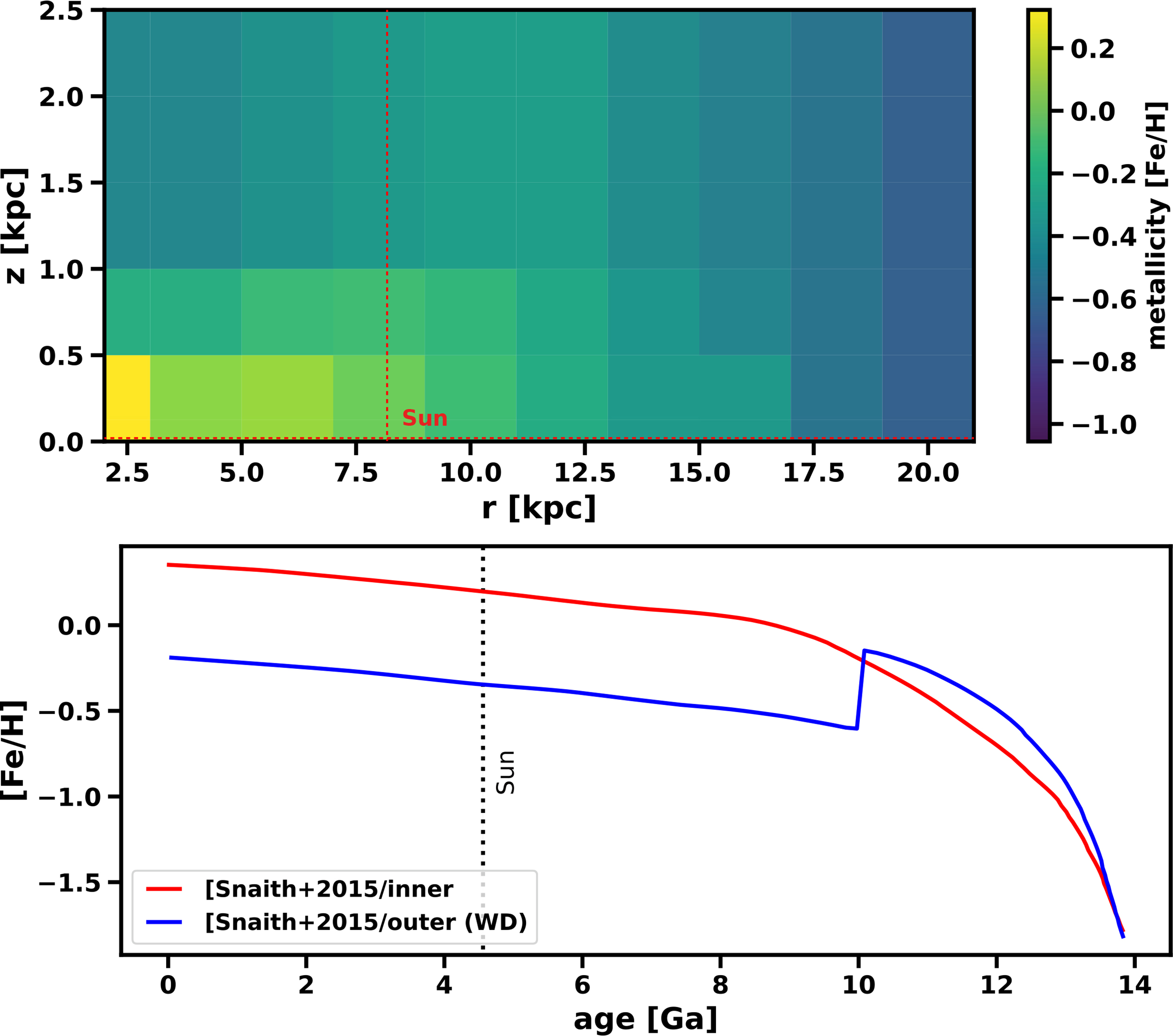
As a final step, we need to implement the actual SFH, that is, the evolution of the SFR of the galactic disk to obtain the distribution of presently existing main-sequence stars as a function of stellar mass and age. For this, we implement the SFH as reconstructed by Snaith et al. (2015) into our nominal case. These authors developed a chemical evolution model to reconstruct the SFH of the galactic disk over time from present-day chemical abundances of the Milky Way’s inner (
The upper panel of Figure 3 shows the best-fit SFH for the inner (solid black line) and outer disks (dashed black line) by Snaith et al. (2015) that we use within our nominal case. For comparison, we also display the reconstructed SFH for the Milky Way by Naab and Ostriker (2006), the cosmic SFH (green line) by Madau and Dickinson (2014), and the SFH of a 2 kpc wide bubble around the Sun (gray line) by Ruiz-Lara et al. (2020). We evaluate how a change in SFH might affect the maximum number of EHs in Section 6.

Upper panel: The normalized best-fit star formation history (SFH) for inner (solid black line) and outer disk (dashed black line) by Snaith et al. (2015), the reconstructed SFH of the Milky Way by Naab and Ostriker (2006), the cosmic SFH (green line) by Madau and Dickinson (2014), and the SFH of a 2 kpc wide bubble around the Sun (gray line) by Ruiz-Lara et al. (2020). Lower panel: Inner and outer SFH by Snaith et al. (2015) renormalized (dotted lines) to only include stars that still reside on the main sequence.
The SFH in the upper panel of Figure 3, however, shows any star that ever existed in the galactic disk. Since we are only interested in those that are still on the main sequence, we need to renormalize the distribution. This can easily be done by excluding any star that already diverged from the main sequence via Equation 8. The lower panel of Figure 3 consequently shows the renormalized SFH for the inner and outer disk as implemented in our nominal case. The distribution, as expected, slightly shifts toward the present day.
As a side note, be aware that the SFH by Snaith et al. (2015) starts at an age of 14 Ga, even though the actual age of the Universe is currently estimated to be around 13.8 Gyr (Planck Collaboration et al., 2020) and the epoch of reionization with the emergence of the first stars might date some few 100 Myr later still (Robertson, 2021), with the oldest galaxies having emerged earlier than about 400 Myr after the Big Bang (Robertson et al., 2022).20 By using this specific SFH, we are stuck with this age determination, but this will not affect our results significantly. A later starting age would potentially decrease the maximum number of EHs further since the earliest stars would have had less time for their XUV flux to decrease (see Section 5.2).
By implementing IMF, SFH, and main-sequence lifetime into our model, we can already derive some interesting numbers even though we did not yet calculate
From all the stars that ever formed within the disk, 91.15(+0.60/−2.04)%21 are yet residing on the main sequence. Within a stellar mass range of
The average initial stellar mass calculated through the IMF is
Finally, only 46.86(+0.48/−3.33)% of the entire stellar mass that has ever been produced within the disk is yet residing on the main sequence, which is in stark contrast to the aforementioned stellar survival rate of 91.15(+0.60/−2.04)%. This illustrates a strong shift toward lower mass stars over time as can also be seen through a change in the relative stellar distribution within the different spectral classes. By considering the canonical IMF with
The relative distribution of stars at the present day as a function of stellar birth age and mass can be seen in Figure 4 for our nominal case. The upper panel shows the relative fraction of stars within age and mass bins of δt = 50 Myr times δM = 0.01
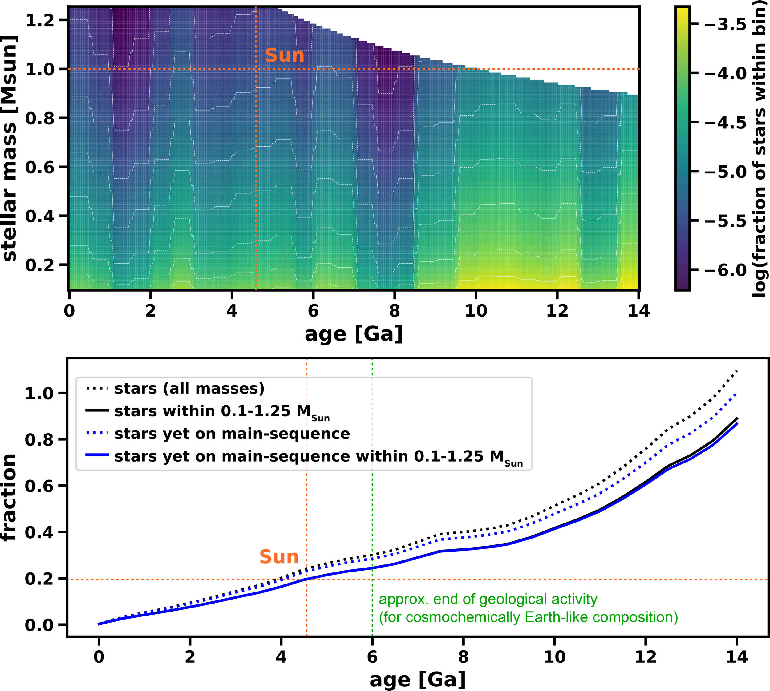
Upper panel: The relative fraction of today’s main-sequence stars between 0.1 and 1.25
According to our nominal case, about 71.5% of all main-sequence stars are older than 6 Gyr. This age is of particular interest since data from coupled galactic chemical evolution and geophysical thermal models indicate that the window for geologically active, cosmochemically Earth-like planets is around 6 Gyr (Frank et al., 2014; Mojzsis, 2021). Older planets might therefore show strong restrictions in maintaining carbon–silicate and nitrogen cycles.
As the evolution of an EH also depends on its location within the galactic disk, we not only need to calculate the number of stars but also their distribution within the disk. For this purpose, we make use of the widely accepted axisymmetric mass distribution and gravitational potential model of the Milky Way by McMillan (2017, 2011). Their model divides the galaxy into 6 axisymmetric components, that is, the bulge, the dark-matter halo, thin and thick stellar disks, H
The density distribution,
In both equations,
Parameters of the Best-Fitting Model for the Galactic Stellar Disks by McMillan (2017), Stellar Disk Mass and Stars (Nominal Case)
By using Equation 10, we can calculate the whole stellar mass,
In this study, it has to be noted that the model by McMillan (2017) assumes no “central hole” for the thin and thick disk. It presumes that the disks extend into the bulge until the center of the galaxy at r = 0 kpc. We therefore have to exclude the central part and start our calculation at
We further need to clarify, which class of objects are included within the stellar mass of the disk. Since McMillan (2017, 2011) gives no further description of the stellar disk mass,
If we divide these numbers by our calculated average stellar mass of
To actually calculate the stellar distribution in the galactic disk, we have to integrate Equation 9 over
We set
Within such boundary conditions (i.e.,

Galactic habitable environment
The concept of the GHZ was first discussed in detail by Gonzalez et al. (2001) and Lineweaver et al. (2004), and refers to regions within a galaxy in which planets can provide a “long-term habitat for animal-like aerobic life” (Gonzalez et al., 2001). As already discussed in Section 4.1 related to the bulge, simulations for the GHZ mostly consider the following three different criteria, that is, (i) high-energetic events that can sterilize a planet and erode its atmosphere, (ii) orbital perturbations of a stellar system, and (iii) the metallicity of the ISM.
The upper panel of Figure 6 shows the probability of a planet being habitable as a function of galactocentric distance for several different GHZ models from the scientific literature. Lineweaver et al. (2004) modeled the evolution of habitability in the Milky Way and considered stellar distribution, metallicity, sufficient time for biological evolution, and the effect of SNs. They found that most habitable environments are within a narrow annulus of 7–9 kpc from the galactic center as schematically and in a simplified manner illustrated by the dashed orange line in Figure 6.25 Between this region and the galactic center, the high-energetic radiation of SNs becomes too strong and frequent to allow for complex life. Farther outside the metallicity becomes so low that the probability of forming rocky exoplanets becomes low as well.
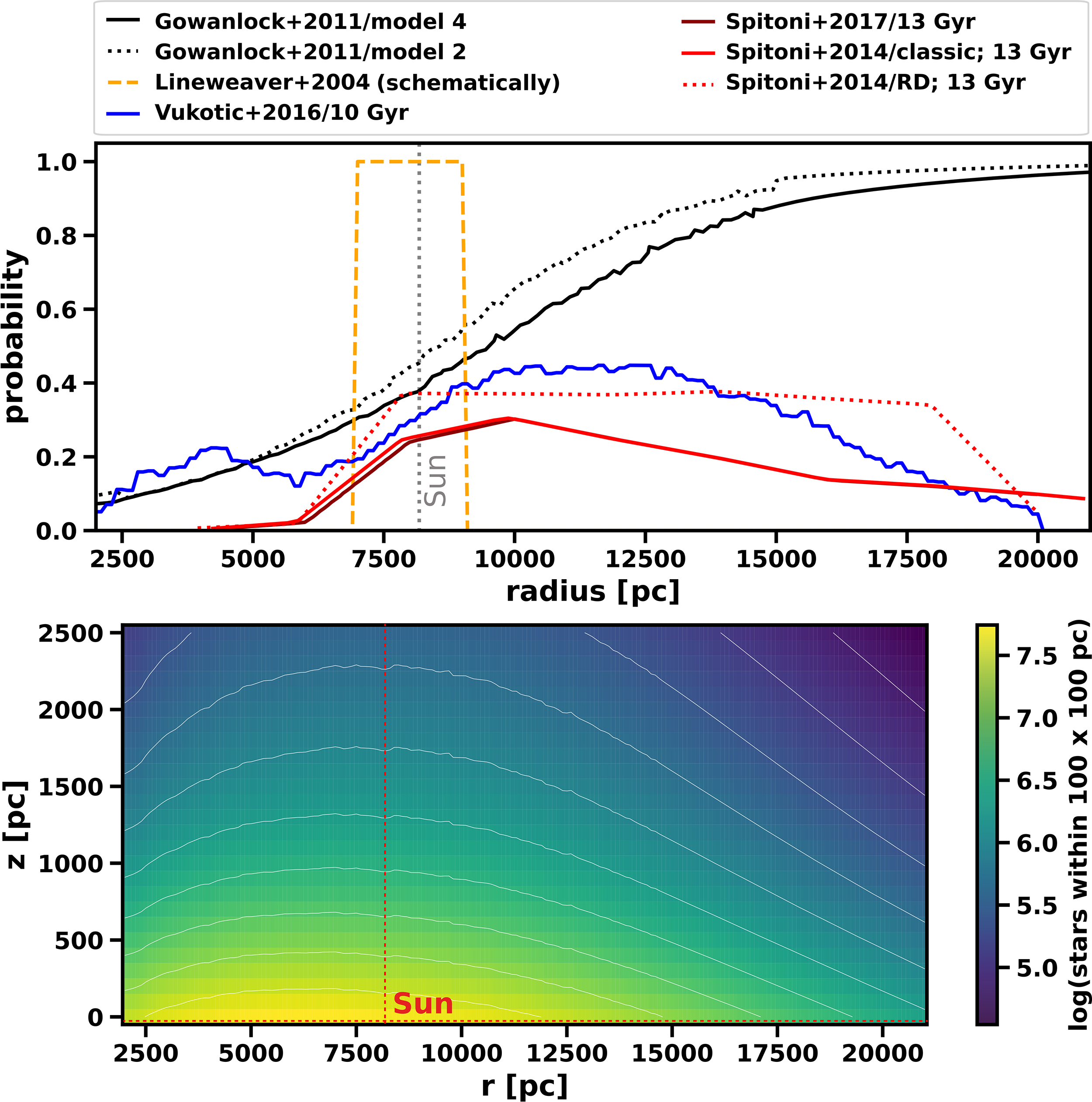
Upper panel: Galactic habitable zones (GHZ) from various studies, which show the probability of being habitable as a function of galactocentric distance. The black lines show the fraction of stellar systems that are not sterilized by supernovae (SNs) in two of the GHZ models (both of them extrapolated from 15000 pc up to 21000 pc) by Gowanlock et al. (2011). The dashed orange line schematically and in a simplified manner illustrates the annular region of 7000–9000 pc from the landmark study by Lineweaver et al. (2004) within which habitable planets are the most likely; note, however, that the GHZ in Lineweaver et al. (2004) is much more complex (see their Fig. 3) and that habitable planets are not restricted to this annulus. The blue line indicates results by Vukotić et al. (2016) for the 10-Gyr-old galaxy based on SN explosions, metallicity, and orbital stability. The red and dark-red lines show different models by Spitoni et al. (2014) and Spitoni et al. (2017) that include SN explosions and the chemical evolution of the Milky Way. Lower panel: Distribution of stars in the r–z plane of the galactic disk that were not sterilized by SNs during the last 4 Gyr based on “model 4” by Gowanlock et al. (2011), that is, the model implemented in our nominal case. Data extracted from: upper panel of Figure 6 by Gowanlock et al. (2011) for the solid black lines (model 2 and model 4); bottom right panel of Figure 5 in Vukotić et al. (2016) for the blue line; Figure 4 and right panel of Figure 11 (dark red lines, both) by Spitoni et al. (2014) for the red solid and dotted lines, respectively; right panel of Figure 5 (yellow line) by Spitoni et al. (2017) for the dark red line; GHZ by Lineweaver et al. (2004) as stated within their article.
The black lines in Figure 6 show the probability of not being sterilized by SNs of types Ia (SNIa) and II (SNII) during the last 4 Gyr in two of the four GHZ models provided by Gowanlock et al. (2011), as derived from the SFH and metallicity gradient modeled by Naab and Ostriker (2006). The dotted black line shows “model 2” by Gowanlock et al. (2011), which is additionally based on the Kroupa IMF and the stellar number density from Carroll and Ostlie (2006), while the solid black line illustrates their “model 4,” which is also based on the Kroupa IMF but takes the stellar number density from Jurić et al. (2008).26 By additionally excluding stars with a metallicity too low to host rocky exoplanets (not displayed in Fig. 6), Gowanlock et al. (2011) further conclude that most habitable planets will be toward the inner galaxy since this galactic region is much more densely populated by stars that have a sufficiently high metallicity to form rocky exoplanets.
To derive the probability distribution of not being sterilized by SNs, Gowanlock et al. (2011) assume that a stellar system must not be sterilized within the last 4 Gyr, so that metazoan life can potentially arise on a planet, a timescale that is simply based on an analogy with the emergence timescale of metazoan life on the Earth. The spatial and temporal occurrence rates of SNIa- and SNII-type SNs in their galactic models were calculated by assuming that stars with a stellar mass of
In this study, we note that such probability distribution may provide relatively conservative assumptions on the lethal effects of SNs. If the putative organisms on a planet evolved and adapted to already harsh radiation environments and/or the emergence of complex life needs less time, it may overestimate the lethal role of high-energetic galactic events. In addition, it must be noted that complete sterilization of a biosphere is relatively unlikely since some extremophiles can withstand high amounts of radiation (Balbi et al., 2020). On the contrary, new simulations, based on the evaluation of SN-emitted cosmic rays (Thomas and Yelland, 2023) and X-rays (Brunton et al., 2023),27 find that SNs might be lethal over even larger galactic distances than initially thought, which could also indicate an underestimate of lethal distances within existing GHZ models. However, the important aspect of high-energetic events for a biosphere relates to the question of whether the planetary conditions can be restored toward habitability in such a way that an extended biosphere can develop afterward. That means that not the entire planet has to be sterilized (including extremophiles) but its biosphere must not recover (see also discussion in Section 4.1).
The upper panel of Figure 6 also shows simulations by Spitoni et al. (2017, 2014), who considered SNs and the chemical evolution of the Milky Way with (solid red line; Spitoni et al., 2014) and without radial gas flow (dotted red line; Spitoni et al., 2014), as well as the effect of dust (solid dark-red line; Spitoni et al., 2017) on the GHZ. After 13 Gyr of evolution, the model without consideration of radial gas flow (solid red line) finds the most habitable region to be within 8 and 12 kpc, while the model that includes radial gas flow enhances the habitability of the outer galactic disk. Similarly, Spitoni et al. (2017) find the galactic disk to be most habitable around 8 kpc within their updated model.
All of the abovementioned models, as well as further research by Morrison and Gowanlock (2015), Forgan et al. (2017), and Spinelli et al. (2021), broadly agree that the Milky Way has the highest probability of providing habitable conditions either around the location of the Sun or, particularly in terms of numbers of habitable planets, toward the inner disk. However, the solid blue line in Figure 6 shows another study by Vukotić et al. (2016) who found that habitability might increase further toward the outer disk, with the peak value to be around 10–15 kpc. As pointed out by these authors, the reason for this discrepancy might be due to the chosen stellar threshold density, SFR, and particularly due to dynamical effects that cause outward migration of metal-rich stars (see also, Gowanlock and Morrison, 2018).
To implement galactic habitable environments into our model, we first consider the effect of SNs on the habitability of the galactic disk based on the GHZ results by Gowanlock et al. (2011) and others. The evolution of metallicity is then implemented separately afterward, as outlined in Section 5.1.2. We further assume orbital perturbations from nearby stars to be negligible within the disk and do not consider the effect of GRBs for estimating the maximum number of EHs (see appended Section 5.1.1).
Finally, we need to note that we do not consider radial mixing of gas and stellar migration within the galactic disk although such processes were likely important for galactic chemical evolution (Minchev et al., 2013; Roškar et al., 2008; Schönrich and Binney, 2009; Sellwood and Binney, 2002; Spitoni et al., 2015). This could affect our results since stars can migrate from more hostile toward more habitable regions and vice versa, thereby affecting the conditions for life within these systems. Based on age–metallicity relationships, it was even suggested (Baba et al., 2023; Lu et al., 2022) that the Sun itself migrated outward from a potential galactocentric birth location around 5 kpc toward its present position at around 8.1 kpc. If so, the Sun would have been born in a region with higher SFRs and SN rates, affecting the evolution of habitability in the solar system. Enhanced SNs and Wolf–Rayet winds, for instance, could explain the increased implantation of short-lived radionuclides into the protoplanetary disk of the Sun (Baba et al., 2023), a potential beneficial feature related to the evolution of EHs (see appended Section 5.1.1). If the solar system remained in the inner disk, however, it could have affected its habitability negatively due to the increased SN rates.28
Implementing
For considering the effect of SNs as part of
For our nominal case, we implement the probability distribution of “model 4” by Gowanlock et al. (2011), which makes use of the Kroupa IMF (Kroupa, 2001) with
The effect of
The highest density of stars that are not affected by SNs within our nominal case can be found at a galactocentric distance of 7.0 kpc, and about 49% of such stars are located farther away from the galactic center than the Sun. In total,
If we change the SFH within our nominal case to the one by Naab and Ostriker (2006) to be in line with the SFH used by Gowanlock et al. (2011) but keep everything else the same, we obtain
As noted above, recent studies by Thomas and Yelland (2023) and Brunton et al. (2023) found that SNs may be lethal over larger distances than initially thought. Thomas and Yelland (2023) calculated that the cosmic ray flux from an average SN can be lethal up to 20 pc instead of 8–10 pc as usually assumed. Depending on the total energy of the SN, its conversion efficiency to cosmic rays, and variations in interstellar transport, the lethal distance estimated by Thomas and Yelland (2023) can vary between 4 and 160 pc. Gowanlock et al. (2011) take 8 pc from Gehrels et al. (2003) as the average lethal distance for an SN with lethal distances varying between about 2 and 27 pc depending on SN type and luminosity. One can therefore expect that implementing the new calculations by Thomas and Yelland (2023) would decrease the number of stellar systems that are not affected by SNs in our model. In addition, Brunton et al. (2023) estimate that the emitted X-ray flux of SNs can be lethal up to 50 pc, an effect that may likely lead to an additional decrease of unaffected systems. However, implementing these recent results into our model is beyond the scope of the present study.
If we finally take into account studies that also include metallicity within their GHZ, the number of stars that can still host EHs decreases significantly and ranges from
The metallicity requirement,
Calculating and implementing
Planet occurrence rates seem to be correlated with the metallicity of the host stars (Adibekyan, 2019; Zhu, 2019; Hansen et al., 2021). Based on observations, Fischer and Valenti (2005) were the first to present a probability relationship between a star’s metallicity, (Fe/H), and the occurrence rate of gas giant planets (GGPs) with orbital periods shorter than 4 years around FGK main-sequence stars, that is,
Based on this relation, Johnson and Li (2012) further suggested that the first Earth-like planets should have formed around stars with a metallicity of
Zhu (2019) and Hansen et al. (2021) further investigated the relationship between planetary radius,
To implement the importance of metallicity (i.e.,
If we did not account for the evolution of galactic metallicity, we would overestimate G- and F-type stars with lower metallicities but at the same time underestimate M and K dwarfs with lower metallicities, since old, low-metallicity stars are predominantly low-mass stars.
To take account of the present-day metallicity, we closely follow Westby and Conselice (2020) and implement the galactic MDFs suggested by Hayden et al. (2015). These authors provide skewed Gaussian metallicity distributions, including mean values, standard deviation, and the respective skewness, for different galactocentric distances within the disk. Similar to Westby and Conselice (2020), we use these values to calculate the galactic probability distribution of stars above a certain metallicity threshold. Since Hayden et al. (2015) only provide data between 3 kpc and 15 kpc, we make use of their fitting relationship for the inner and outer skirts of the disk, that is,
Upper panel: The metallicity (Fe/H) distribution of the present-day galactic disk according to Hayden et al. (2015). Closer than r = 3 kpc and beyond r = 15 kpc the value for (Fe/H) was extrapolated with the fitting function provided by Hayden et al. (2015); for z > 2 kpc it was further assumed to be the same as for z < 2 kpc. Lower panel: Evolution of (Fe/H) for the inner (red; model with dilution; see text) and outer disk (blue) according to the best-fit model by Snaith et al. (2015).
As we further account for the metallicity evolution of the Milky Way, we implement the best-fit (Fe/H)-age tracks provided by Snaith et al. (2015) for the inner and outer disk, which correlate with the best-fit SFH from their chemical evolution model. These tracks can be seen in the lower panel of Figure 7 where “with dilution” denotes their best-fit model for the outer disk. For this, Snaith et al. (2015) assumed a galactic accretion event at 10 Ga that diluted the in situ gas of the outer disk with primordial gas to match the age-metallicity and age-α observations by Haywood et al. (2013). It is worth noting that a similar dilution effect was later also considered by Spitoni et al. (2019, 2020, 2021) and Lian et al. (2020b, 2020a) within their chemical evolution models for reproducing the abundance ratio of (α/Fe)31 versus (Fe/H) in Apache Point Observatory Galactic Evolution Experiment32 stars in the outer disk.
To combine the evolutionary tracks from Snaith et al. (2015) with the present-day distribution from Hayden et al. (2015), we renormalize the (Fe/H)-age tracks for inner and outer disk with the present-day values of the different Milky Way regions so that the evolving metallicity of the best-fit model by Snaith et al. (2015) will reach the certain regional (Fe/H)-values as observed by Hayden et al. (2015). The average metallicity of all stars within a certain region will hence be renormalized to meet the present-day metallicity value of this respective region. If we generally average over the (Fe/H)-values provided in Hayden et al. (2015) for the outer disk region between 7 and 15 kpc (for a disk height
The upper panel of Figure 8 shows the probability of any presently existing star to be above the threshold value of our nominal case, that is,

Upper panel: The present-day probability for a certain star to be above a metallicity threshold of
The lower panel of Figure 8 illustrates the age distribution of remaining stars that fulfill our nominal case metallicity threshold of
In total, 69.3% of all remaining stars meet the metallicity threshold of
Finally, 76.69(+1.00/−0.45)% of the remaining stars are low-mass M dwarfs, which is a slightly lower value than for the entirety of GHZ stars, for which it is 77.27(+0.77/−0.0)%. This small shift relates to the fact that the metallicity of the ISM has been increasing since the galaxy’s birth, thereby implying that M dwarfs are, on average, below the threshold more often than heavier stars. This can be seen in Figure 9, where the upper panel illustrates the stellar fraction above the respective metallicity threshold

Upper panel: The fraction of stars above the different metallicity thresholds
As a final note related to metallicity, we point out that the occurrence rate of rocky exoplanets will not only depend on a lower metallicity cutoff. Their formation probability may also decrease for high metallicities. This seems to be likely due to (i) a rise in the occurrence rates of hot Jupiters (Buchhave et al., 2018; Osborn and Bayliss, 2019) and warm, dynamically active giant planets (Schlecker et al., 2021) with increasing metallicity, and (ii) an increase in rocky building blocks that may lead to the growth of more massive planets with hydrogen-dominated atmospheres. Through assuming (i) and the related destruction of rocky exoplanets by migrating hot Jupiters, Prantzos (2008) and subsequently Carigi et al. (2013), used Equation 12 by Fischer and Valenti (2005) to calculate the probability of a star hosting Earth-like planets but not hot Jupiters, thereby taking into account a potential lower probability of rocky exoplanets around high-metallicity stars. However, Spitoni et al. (2014) already pointed out that this assumption might be questionable since the relationship by Fischer and Valenti (2005) covers any GGPs with orbital periods shorter than 4 years.35 Since GGPs on wider orbits (as is the case in the solar system) will not necessarily destroy or disturb Earth-like planets in circumstellar HZs, one may expect that applying such relationship could slightly underestimate the occurrence rate of rocky exoplanets around high-metallicity stars (see also Fig. 8 in Carigi et al., 2013), whereas the opposite may hold for neglecting any such relationship (as in our model). This reasoning, however, is only based on argument (i), while the relevance of argument (ii) cannot be properly assessed with our present scientific knowledge.
One of the most important requirements for an EH, even though it is often overseen or ignored, is the long-term stability of its N2-O2-dominated atmosphere against atmospheric escape to space on the one hand (i.e., the lower limit
To meet the lower limit, any atmospheric sinks such as thermal and nonthermal escape to space must be either negligible or at least smaller than any atmospheric sources (e.g., volcanic degassing or biological processes) that would otherwise replenish nitrogen and oxygen into the atmosphere. In this study, thermal escape is mostly driven by the incident XUV flux36 of the host star, which heats and expands the upper atmosphere (see appended Section 1.2), and thereby removes neutral gas via a hydrostatic or hydrodynamic flow into space (Erkaev et al., 2013; Johnstone et al., 2019a, 2021b; Kubyshkina and Vidotto, 2021; Tian et al., 2008a). Nonthermal escape, on the contrary, mostly removes ionized gas from the atmosphere and is mainly driven by CMEs and the stellar wind of the star and/or the polar outflow from a planet’s own magnetosphere (Airapetian et al., 2017; Dong et al., 2017b, 2018, 2019; Garcia-Sage et al., 2017; Khodachenko et al., 2007; Lammer et al., 2007; Scherf and Lammer, 2021).
The upper limit,
In the appended Sections 1.1 and 1.2, we discuss the scientific background of stellar evolution, with a particular focus on the relationship between stellar mass, rotational and XUV flux evolution (Section A.1), and the fundamental role of the stellar radiation (XUV flux and flares) and plasma environment (stellar winds and CMEs) for the stability of Earth-like atmospheres and the destruction of ozone (Section A.2). The results presented in these appended sections indicate the importance of considering the evolution of the entire radiation and plasma environment of the various stellar spectral classes. In this study, however, we only consider the role of the stellar XUV flux, but neither include (super)flares nor the role of nonthermal escape into our model. For the latter, the role of intrinsic magnetic fields for atmospheric protection is by now insufficiently investigated and there are no quantifiable model approaches that can be included in our framework, particularly for the evolution of stellar winds and CMEs on stars other than solar-like ones. However, this is an important topic, and we therefore strongly encourage the reader to consult these appended sections.
In the next section, we derive a distribution of stars that can presently host HZCL planets with thermally and climatically stable N2-O2-dominated atmosphere by including the aforementioned lower and upper limits. The stellar XUV flux evolution as a function of stellar mass will serve as a lower threshold by providing lower age limits, for which the XUV flux has declined below a specific threshold level. The bolometric luminosity,
The lower stellar limit,
Implementing
A star’s XUV irradiation is absorbed in the upper atmosphere of a planet, which leads to the heating and expansion of its thermosphere (see Fig. 35 in the Appendix). As we detail in the appended Section 1.2, this effect can be specifically important for Earth-like atmospheres, for which XUV surface fluxes only 5 to 6 times as high as received by today’s Earth will be enough for the atmosphere to expand adiabatically and to erode into space within a few Myr (Johnstone et al., 2021b; Tian et al., 2008a). Since CO2 serves as an infrared coolant (Johnstone et al., 2021b; Kulikov et al., 2007; Lichtenegger et al., 2010), it can prolong the thermal stability of Earth-like atmospheres and we derive certain stability thresholds for nitrogen-dominated atmospheres with maximum mixing ratios of
For implementing
Through this approach, we exclude any star for which
We focus on the HZCL since this concept provides important boundary conditions for our model. Schwieterman et al. (2019a), and more recently Ramirez (2020), define the HZCL (or CLHZ as abbreviated by Ramirez, 2020) as the zone around a star where (i) liquid water can exist at a planet’s surface and (ii) the CO2 partial pressure is below the toxicity limit for complex life (see Section 3.2.5). Both studies find a partial pressure of pCO
Schwieterman et al. (2019a) provide HZCL boundaries for three different values of the CO2 partial surface pressure, that is, pCO
Since we are interested in the maximum number of EHs, that is, HZCL planets that can host N2-O2-dominated atmospheres with minor amounts of CO2, we can combine the results obtained by Johnstone et al. (2021b) on the stability of N2-dominated atmospheres with the concept of the HZCL. For this, we assume any planet to be in the middle of the HZCL even though the actual positions of HZCL planets will certainly vary over its entire orbital range. However, planets inside the mean HZCL distance,
Similarly, we assume that all planets have a mass of M
pl = 1.0 M⊕ since this is the mass for which reliable simulations are available. Planets with higher masses than the Earth will tend to grow faster to reach such a high mass, and the more massive a planet, the likelier it will become that any accreted primordial atmosphere cannot be lost afterward. The so-called Fulton Gap (Fulton et al., 2017; Fulton and Petigura, 2018, see also Section A.2) further supports the hypothesis that planets of a certain mass/radius will tend to host a primordial atmosphere while planets with a radius of
Another upper mass limit can be derived from the degassing of volatiles from a planet’s interior and, potentially, its tectonic regime. While Valencia et al. (2007) and van Heck and Tackley (2011) find that plate tectonics might be equally or more frequent on super-Earths, several other studies conclude that the opposite might be true (Miyagoshi et al., 2015; Noack and Breuer, 2014; O’Neill and Lenardic, 2007). In addition, Noack et al. (2017) and Dorn et al. (2018) for stagnant-lid, and Kruijver et al. (2021) for plate tectonic planets, found that the degassing of volatiles will start to be significantly reduced for planets with
On the other side of the mass scale, small-mass planets will not be able to hold on to an N2-dominated atmosphere. A Mars-mass planet around a G-type star might already be too small to assure the long-term stability of such an envelope and even more massive planets might struggle to keep such an atmosphere, particularly for K and M dwarfs. In fact, nonthermal atmospheric escape tends to reach maximum loss rates for a planetary radius of
These arguments exemplify that for both sides of the mass distribution, planets will become inhospitable to complex life for certain mass limits. However, these upper and lower limits are not (yet) strictly definable, and their mean value might diverge from
As a first step for implementing the XUV limit,
We vary between Moist Greenhouse and Runaway Greenhouse limits as the inner boundary, which coincide with
We substitute the outer boundary of the HZ with the HZCL definitions by Schwieterman et al. (2019a) and Ramirez (2020). While Schwieterman et al. (2019a) give the corresponding values for a, b, c, and d, we directly take
For our nominal case, we take the outer HZCL boundary by Ramirez (2020). By additionally taking the Runaway Greenhouse limit by Kopparapu et al. (2014) as the inner boundary, this results in a mean HZCL distance of
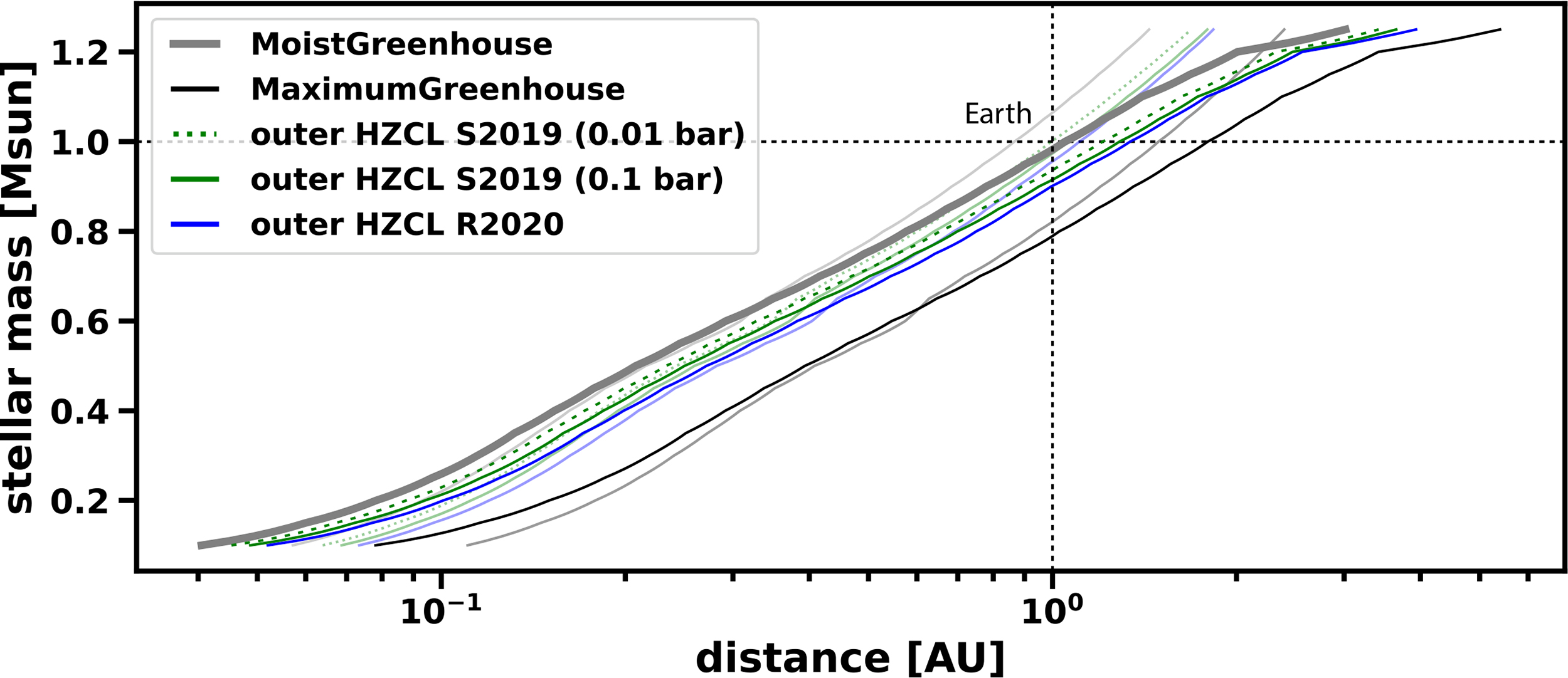
The inner habitable zone (HZ) boundary (thick gray line) of the HZ according to the Runaway Greenhouse threshold and several different outer boundaries, that is, the HZ of complex life (HZCL) for pCO
To be consistent with the outer HZCL boundary in Ramirez (2020), we assume a maximum of pCO
For our minimum case, we, consequently, take into account only the X-ray part of the spectrum with
Figure 11 shows the X-ray (upper panel) and XUV surface flux (lower panel) at
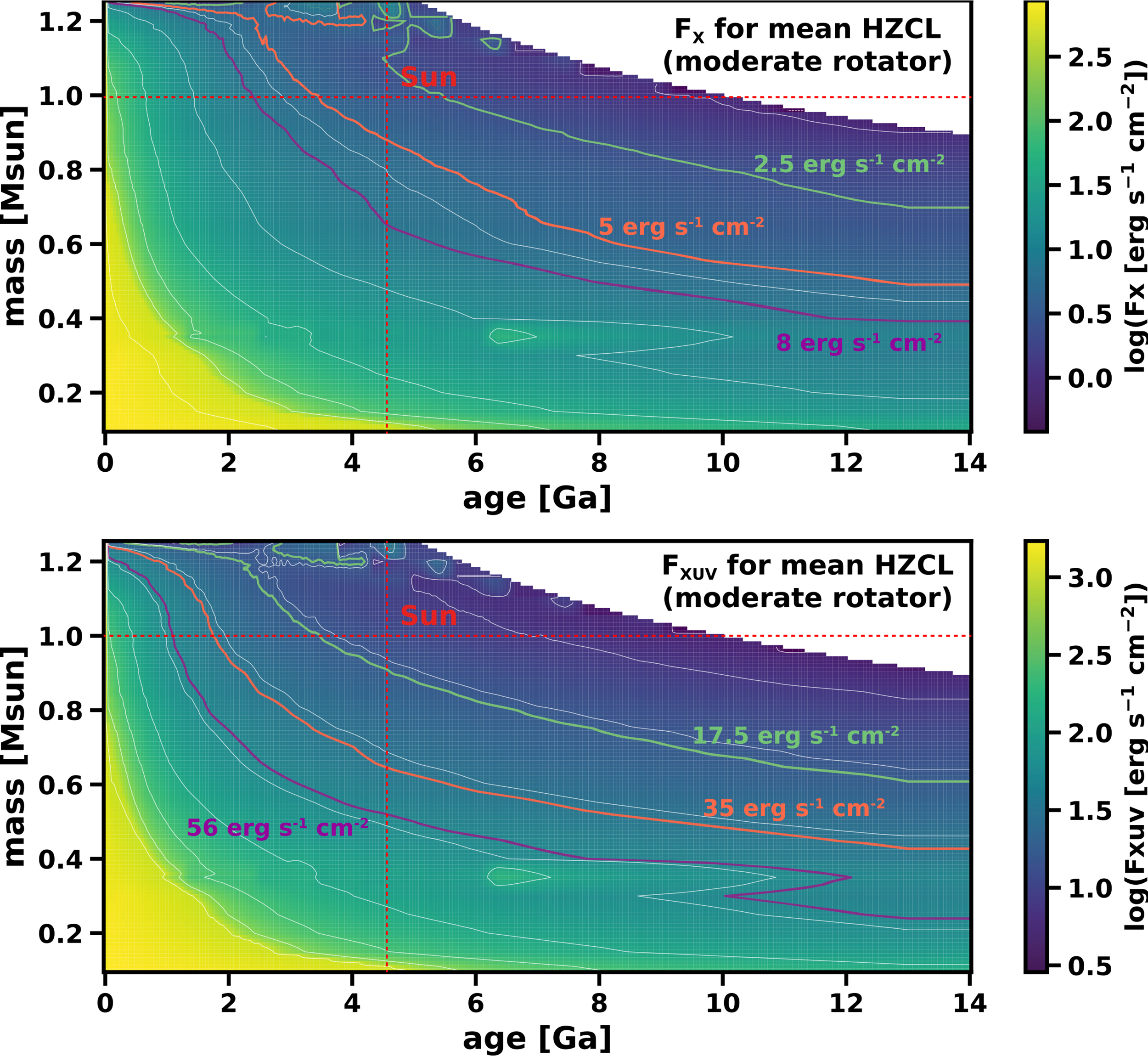
Upper panel: The stellar X-ray surface flux,
It has to be noted, however, that Figure 11 only illustrates the 50th percentile of the stellar distribution, that is, the so-called moderate rotators. Stars with the same mass but at a lower percentile of the rotational distribution will rotate slower (such as the so-called slow rotator at the 5th percentile) and therefore reach any surface flux threshold earlier than the 50th percentile. Conversely, any star that rotates faster will fall below such value later. To account for this effect, we implement the entire stellar rotational distribution, as it can be calculated with Mors, and distribute all stars evenly over all percentiles.
Figure 12 illustrates the age at which each percentile (from 0 to 100th) of each stellar mass (with
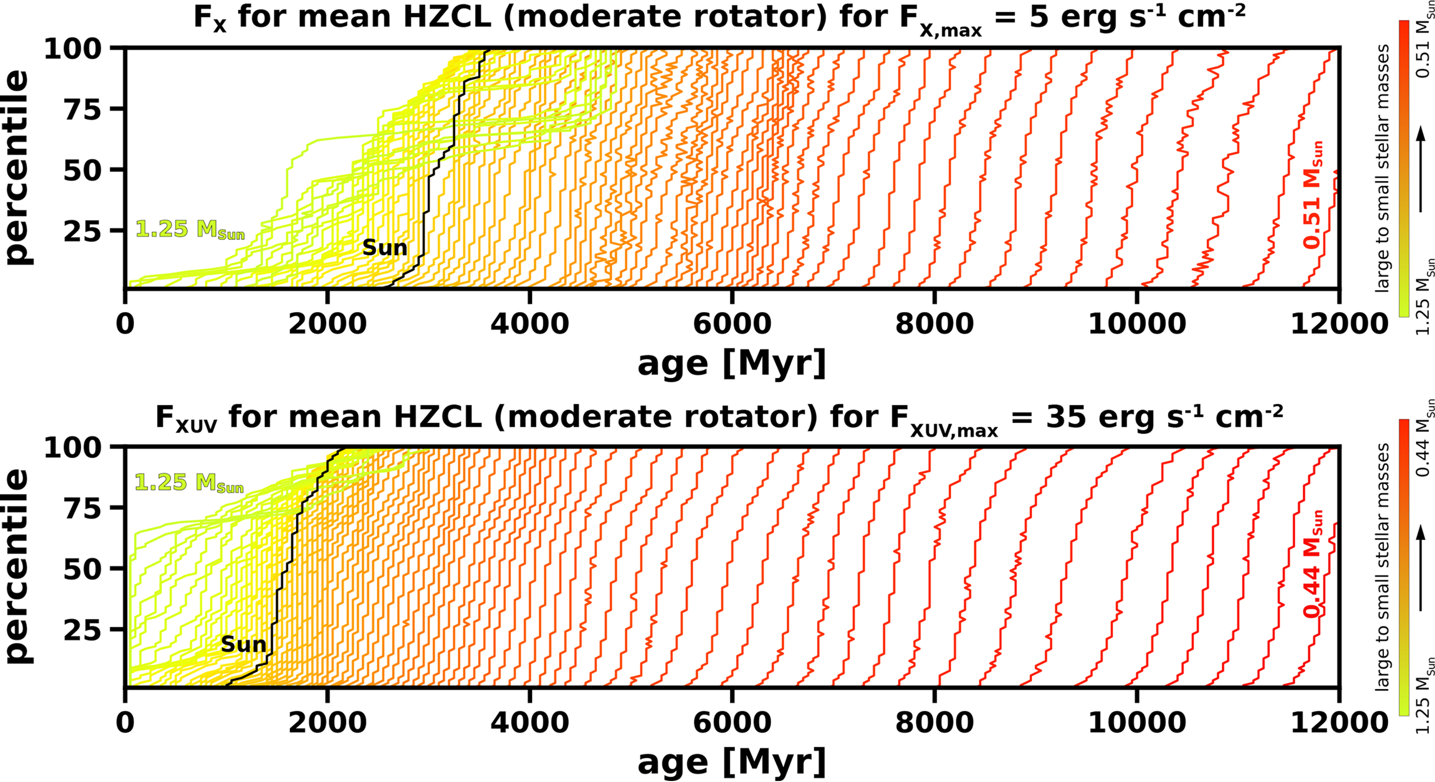
The stellar ages at which the X-ray (upper panel) and XUV surface flux (lower panel) at
With the Runaway Greenhouse limit from Kopparapu et al. (2014) and the pCO2 = 0.1 bar limit from Ramirez (2020) as the inner and outer HZCL boundaries, respectively, and by taking account of the entire stellar rotational distribution, we find that
As a side note, if we change the outer HZCL boundary of our nominal case from Ramirez (2020) to Schwieterman et al. (2019a), the number of suitable stars decreases from
Figure 13 shows the number of remaining GHZ stars that are above the lower limit,
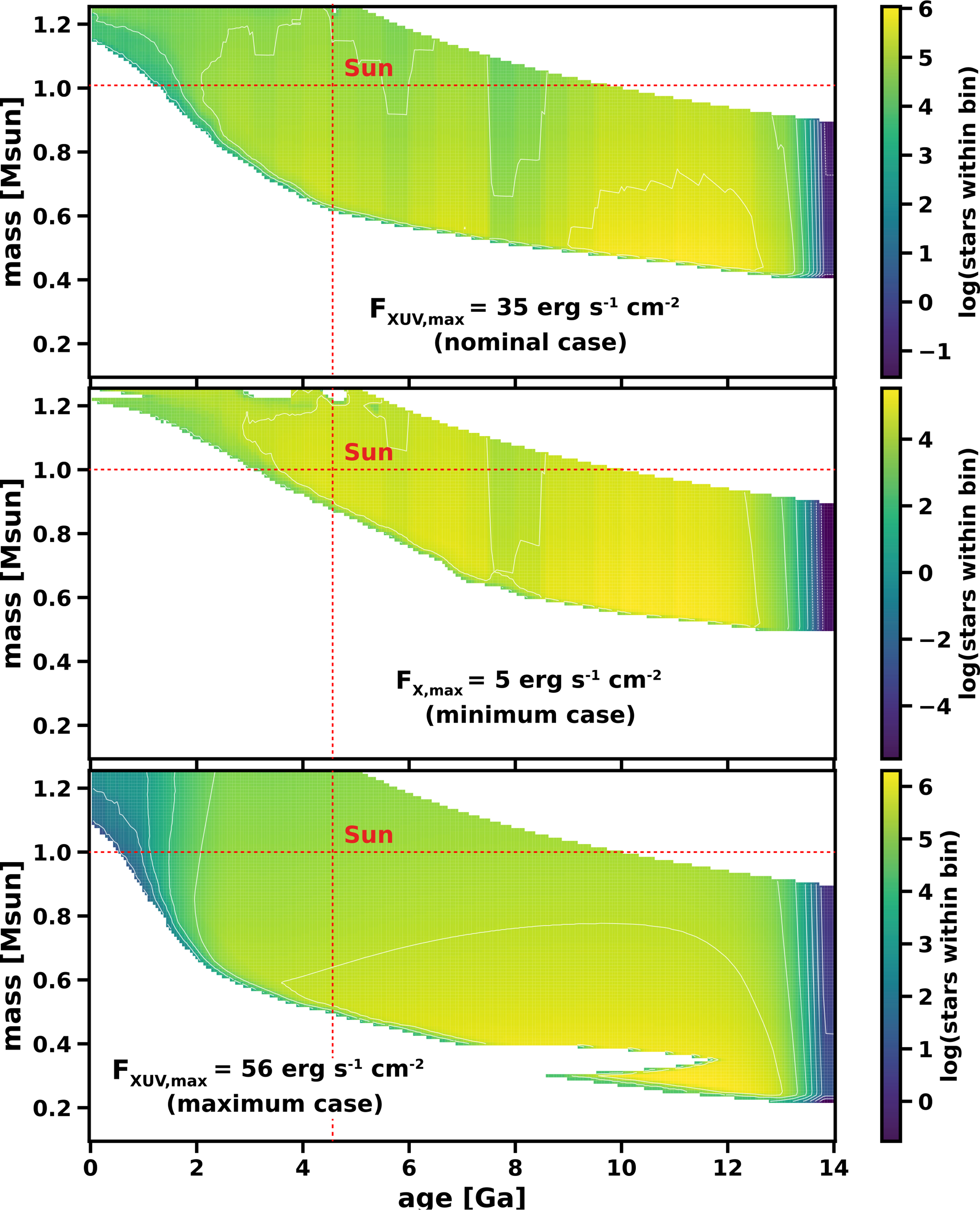
The number of remaining GHZ stars that are above the lower limit,
The lower limit therefore strongly affects the relative fractions of the different spectral classes, much more so than the metallicity threshold. Only 0–22.36% of the remaining stars will be M dwarfs, while K dwarfs suddenly hold the majority with 53.38–68.66%. The relative fraction of G and F stars also rise significantly, that is, from 4.26–4.76% and 1.12–1.49% to 18.09–35.54% and 4.36–11.08%, respectively.
Figure 14 illustrates this distribution. In this study, the upper panel depicts our nominal case and shows the number of stars by spectral class that still meet all requirements as a function of birth age. At maximum, only old M dwarfs remain part of the sample (for the minimum case, no M dwarfs remain, not even old ones), while the distribution shifts toward younger ages for earlier spectral classes. This is particularly interesting because any N2-dominated atmosphere must be outgassed at an age when the star already allows for its thermal stability. A geologically active planet must therefore be a prerequisite for allowing the buildup of a stable atmosphere. As already briefly discussed in Section 4.2.4, however, this may not be the case for planets older than about 6 Gyr (Frank et al., 2014; Mojzsis, 2021). Any M dwarf still part of the distribution has an age much older than the Sun and even older than ∼6 Gyr, indicating that any geological activity on planets orbiting these old stars may already have vanished millions or even billions of years ago, at least for cosmochemically Earth-like planets.
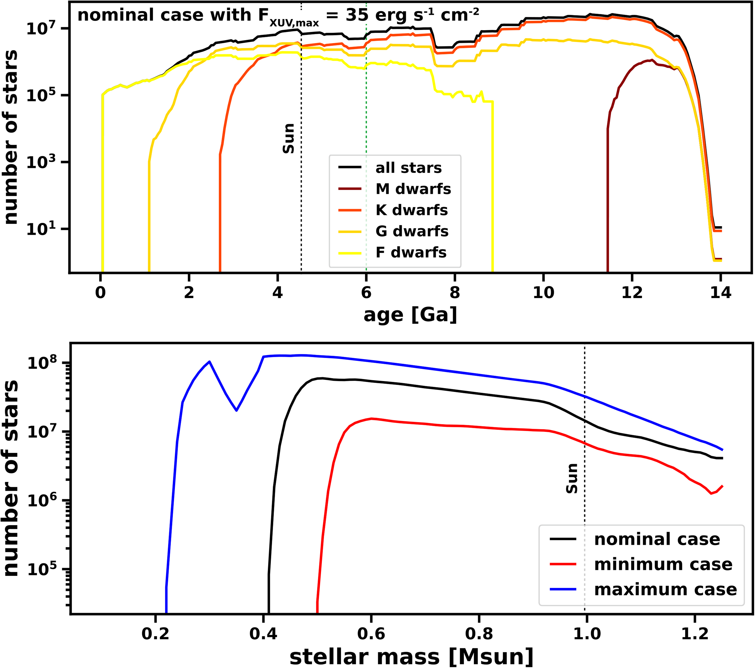
Upper panel: The number of remaining GHZ stars that are above the lower limit,
The lower panel of Figure 14 illustrates nominal, minimum, and maximum cases for
The numbers presented above, however, are for N2-O2-dominated atmospheres with
By applying this criterion, only
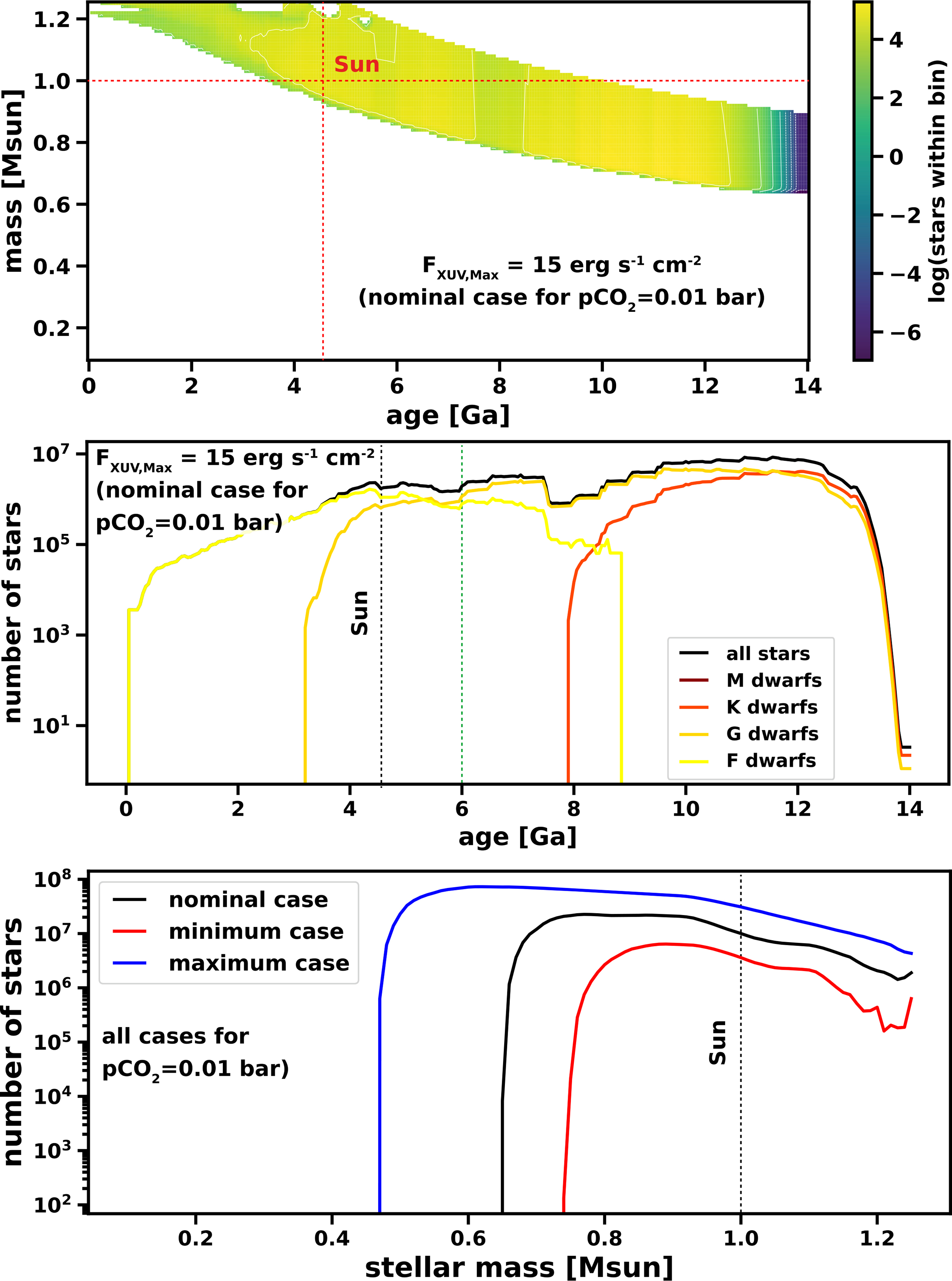
Our nominal case for an N2-O2-dominated atmosphere with
We emphasize that the actual number of stars suitable to host planets with N2-O2-dominated atmospheres will likely be lower, independent of the maximum level of pCO2 chosen. Our calculation of the lower limit neither includes the effect of superflares nor nonthermal escape, the latter of which is triggered through a star’s stellar wind and CMEs. Since these processes are important particularly around M to late K dwarfs, these will further reduce the number of small-mass stars being part of the remaining stellar distribution. EHs around M- and late K-type dwarfs should, therefore, be exceedingly rare.
Implementing
For the upper limit,
We subsequently denote the upper limit simply as
While Kopparapu et al. (2013) calculated Moist Greenhouse and Runaway Greenhouse limits to be at
We investigate
Figure 16 illustrates the stable HZCL boundaries for a time when slow, moderate, and fast rotators fall below the threshold values for the lower limit,
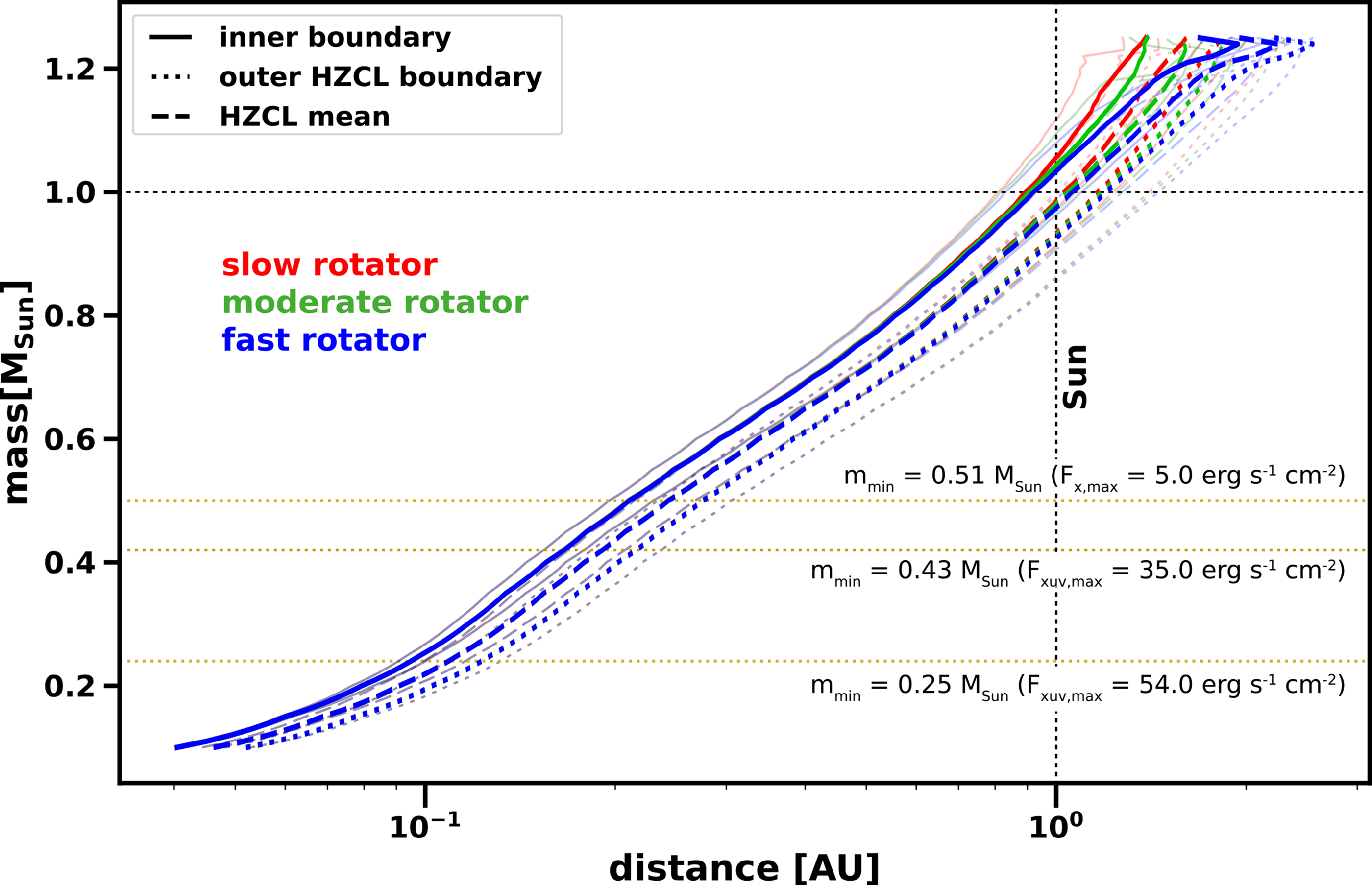
The stable HZCL boundaries for slow, moderate, and fast rotators with
Similar to the lower limit variation, we also change the respective thresholds for the upper limit,
Figure 17 illustrates the ages at which slow, moderate, and fast rotators fall below the lower limits and surpass the upper limits, that is,
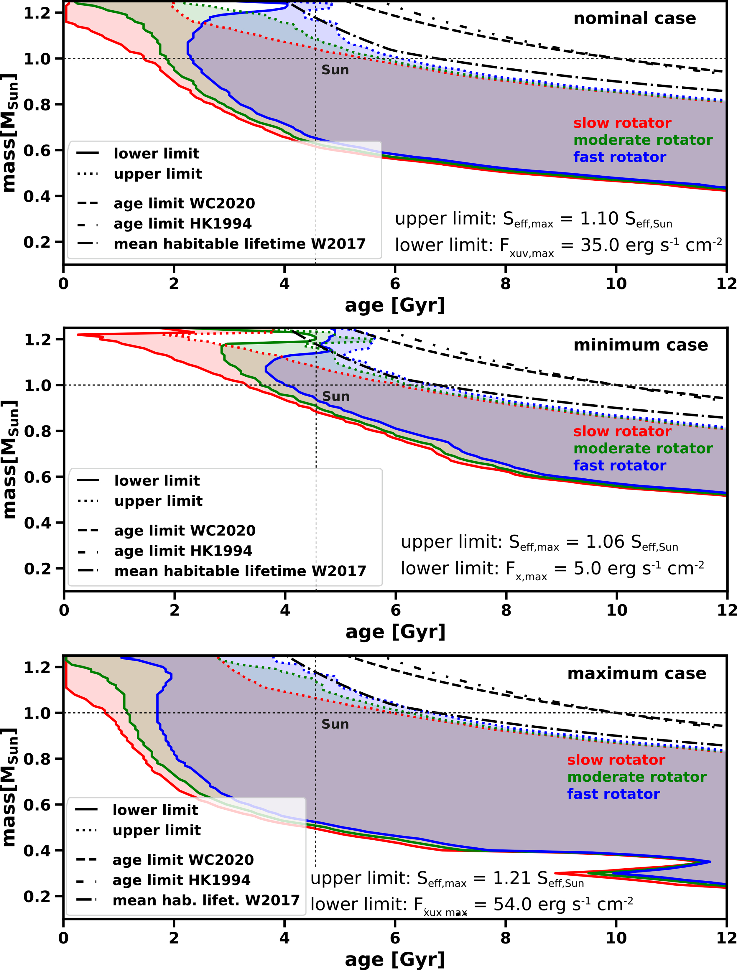
The ages when slow, moderate, and fast rotators fall below the lower and surpass the upper limits, that is,
However, for our nominal case with

The distribution of remaining stars as a function of stellar mass and age, including
It can also be seen in Figure 17 that the specific type of calculation for the main-sequence lifetime, as already introduced in Section 4.2.2, does not influence our final results since the habitability lifetime of EHs will always be shorter than the main-sequence lifetime of the respective star. It happens, however, that the habitable area might intersect with the mean habitable lifetime for intelligent observers from Waltham (2017). This is not surprising as this author’s power law fits define a typical habitable lifetime that is highly dependent on the mean habitable lifetime of various locations in the HZ. The further outward our actual HZCL shifts because of a decrease in the lower threshold value,
This can specifically be observed if we restrict the maximum atmospheric mixing ratio to
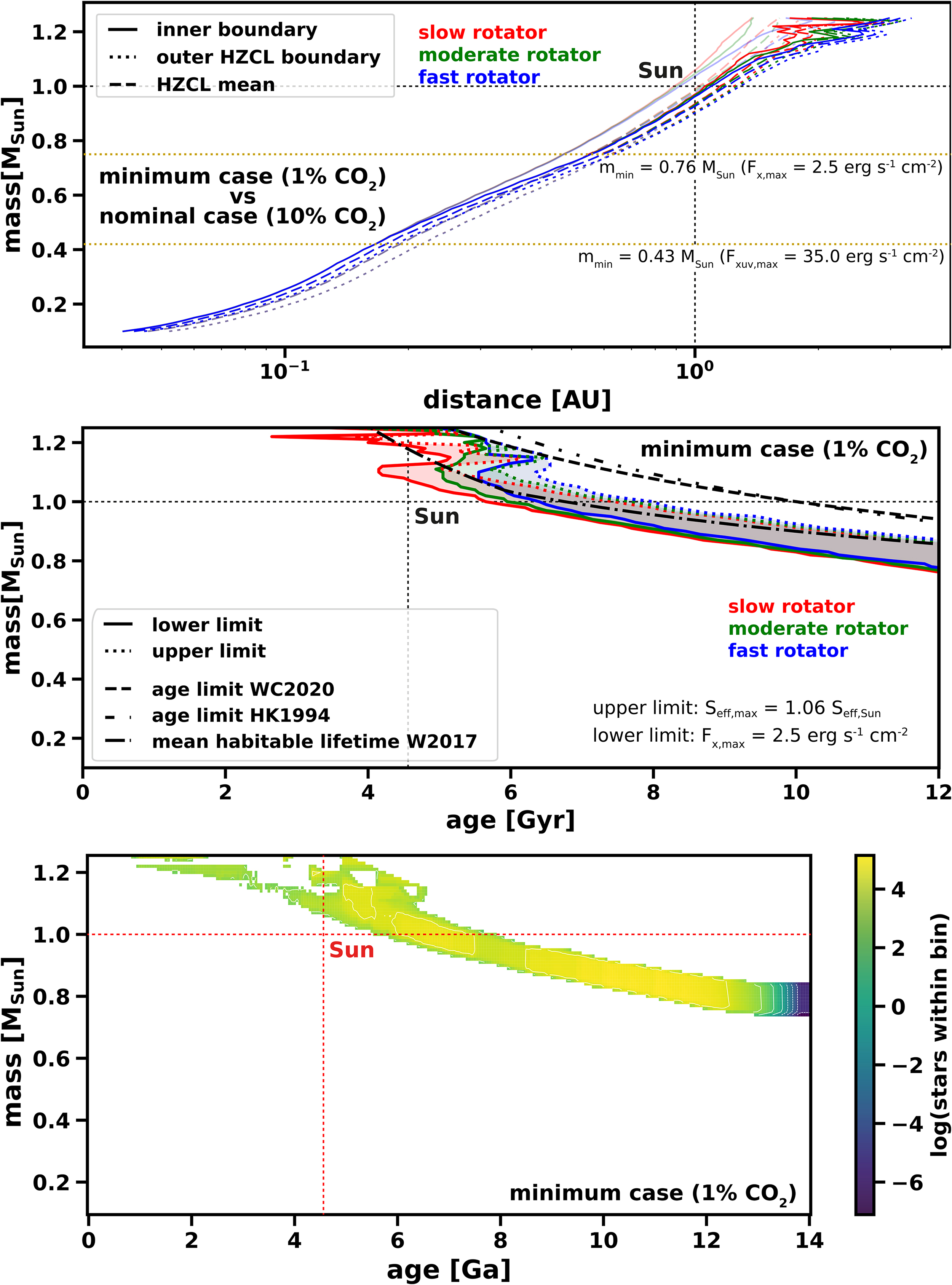
The minimum case for an N2-O2-dominated atmosphere with
An additional problem that may occur for stars with
Finally, we emphasize that the actual upper limit may be determined not by the bolometric luminosity of the parent star, but by the properties of the planet itself. Even though such an upper limit would then be part of
However, CO2 levels might not be the only atmospheric threshold that could be reached before the Moist Greenhouse limit. As Ozaki and Reinhard (2021), who couple carbon, oxygen, phosphorus, sulfur, and methane cycles in their model together with the evolution of the Sun, point out that the Earth’s atmosphere will be deoxygenated to an O2 content of less than 1% of the PAL probably before the Moist Greenhouse limit is reached. Within their simulations, 1% PAL and 10% PAL are achieved in 1.08 ± 0.14 Gyr and 1.05 ± 0.16 Gyr, respectively, largely due to an increase in surface temperature and a prompt halt of photosynthesis, the latter related to the CO2 limits mentioned above (Ozaki and Reinhard, 2021). A similar outcome has been found by Lingam and Loeb (2021), who calculate that the net primary productivity, that is, the net production of organic carbon within a biosphere, will decline steeply toward <10% of the modern value at the time the Runaway Greenhouse state is reached, which is due to the related increase in the average surface temperature. Importantly, this will be accompanied by a strong decline in atmospheric O2 since the oxygen sinks will outcompete its sources, thereby leading to the extinction of advanced animal life well before the ocean begins to evaporate.
One should keep such limits in mind and be aware that the Moist Greenhouse or even the Runaway Greenhouse limit will not be the limiting factor that sets an end to Earth’s complex life biosphere. This will be extinct well before these limits are reached.
As derived step by step in the preceding subsections, not every star with
Avoiding sterilization by nearby SNs (Section 5.1.1)
Depending on our specific case, ∼22–30% of all disk stars (and ∼27–30% of all disk stars in the mass range) fulfill such requirement. Note that this criterion is particularly important for complex and/or surface life, while a microbial or subsurface habitat may require less strict conditions. If organisms on other worlds evolve to adapt to harsh radiation environments and/or complex life requires less time to develop, this requirement could be met by more stellar systems. SNs are, however, not the only high-energy events. GRBs or sudden outbursts of the central SMBH can further reduce the fraction of stars around which a complex biosphere may survive.
Surpassing the metallicity threshold (Section 5.1.2)
Only stars surpassing a certain metallicity threshold allow for the accretion of rocky exoplanets. Depending on the chosen threshold, ∼39–86% of all remaining stars meet this requirement. However, this does not cover the potential upper metallicity threshold above which planets may grow too quickly to allow EHs to form.
The stellar lower limit (Section 5.2.1)
The short-wavelength radiation of young and/or lower mass stars may be too high to allow for the thermal stability of N2-O2-dominated atmospheres. Depending on the chosen threshold, this lower limit is met either by ∼7–27% or ∼2–13% of the remaining sample of stars, depending on whether the atmospheres have maximum CO2 mixing ratios of 10% or 1% CO2, respectively. However, energetic flares and nonthermal escape through stellar winds and CMEs—effects we do not consider—will further reduce the number of stars surpassing this critical and often overseen requirement. Importantly, the number of suitable stars is lower for atmospheres with lower CO2 mixing ratios because their thermal stability is also lower.
The stellar upper limit (Section 5.2.2)
This necessary requirement considers the increase of bolometric luminosity, a fate that will ultimately render any planet uninhabitable. Between ∼79–91% and ∼57–79% of all remaining main-sequence stars are below the chosen stellar surface fluxes for atmospheres with 10% and 1% CO2, respectively, thereby meeting this requirement. Be aware, however, that some planetary parameters (e.g., the halt of photosynthesis) can render an EH uninhabitable even before its heat death.
We must consider the specific stellar mass range that can provide habitable conditions. Even though we predefined a range of
By combining all criteria, a maximum of 2.07(+4.11/−1.60)% of all disk stars provide an appropriate environment for hosting a stable N2-O2-dominated atmosphere with
The Effect of the Necessary Requirements onto
The Effect of the Necessary Requirements onto
For an N2-O2-dominated atmosphere with
Same, but with

The number of remaining stars as a function of necessary requirements feeding into
So, although we obtain a total of
Finally, Figure 21 illustrates the distribution of the remaining stars that are potentially able to host EHs, that is, of
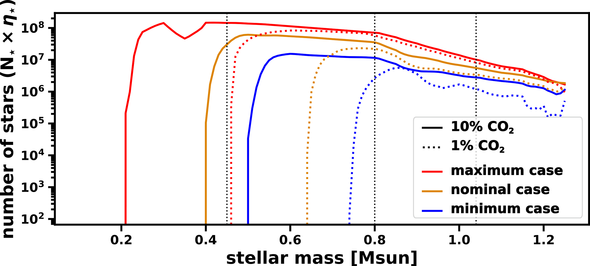
The distribution of the remaining stars that are potentially able to host Earth-like habitats (EHs,) that is, of
The planet occurrence rate of rocky exoplanets within the HZCL,
The occurrence rate,
Calculating and implementing
Values for
To fit the distribution of Kepler planets, several studies (Mulders et al., 2018; Pascucci et al., 2019) assume that the occurrence rate distribution can be described by a separable function in orbital period,
Here,
Mulders et al. (2018) found the respective breaks to be at
To recalculate
By normalizing Equation 16 such that
For the orbital period distribution function,
The maximum radius for our nominal and minimum cases (again for both
As Chen and Kipping (2017) point out, their derived transition from rocky to neptunian at
Nevertheless, it seems reasonable to use the value of Chen and Kipping (2017) for
However, for our two maximum cases, we implement a maximum radius of
The minimum radius,
To summarize, the minimum and maximum radii for our nominal, minimum, and maximum cases with
Figure 22 and the right column of Table 12 compare different
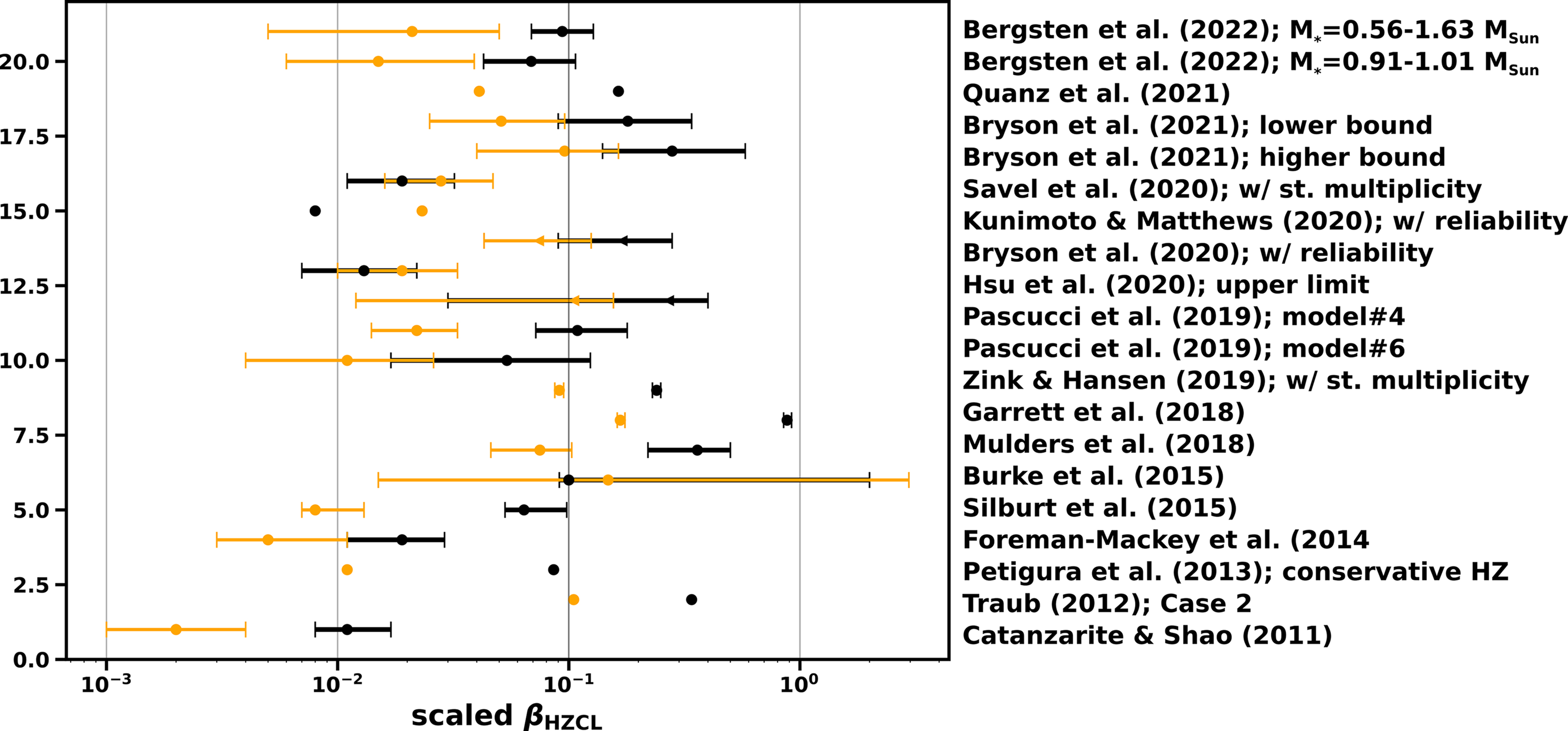
Different values for planet occurrence rates around solar-like stars from the literature (black points and error bars) for the same studies and boundary conditions as listed in Table 12. The orange points and error bars display the calculated values for
For our two nominal cases, we take the
Before implementing
We then let the occurrence rate increase linearly as a function of stellar effective temperature,
If we implement
By only taking an account of stars with sufficient metallicity, the corrected
As exemplified in Figure 22 and Table 12, converting
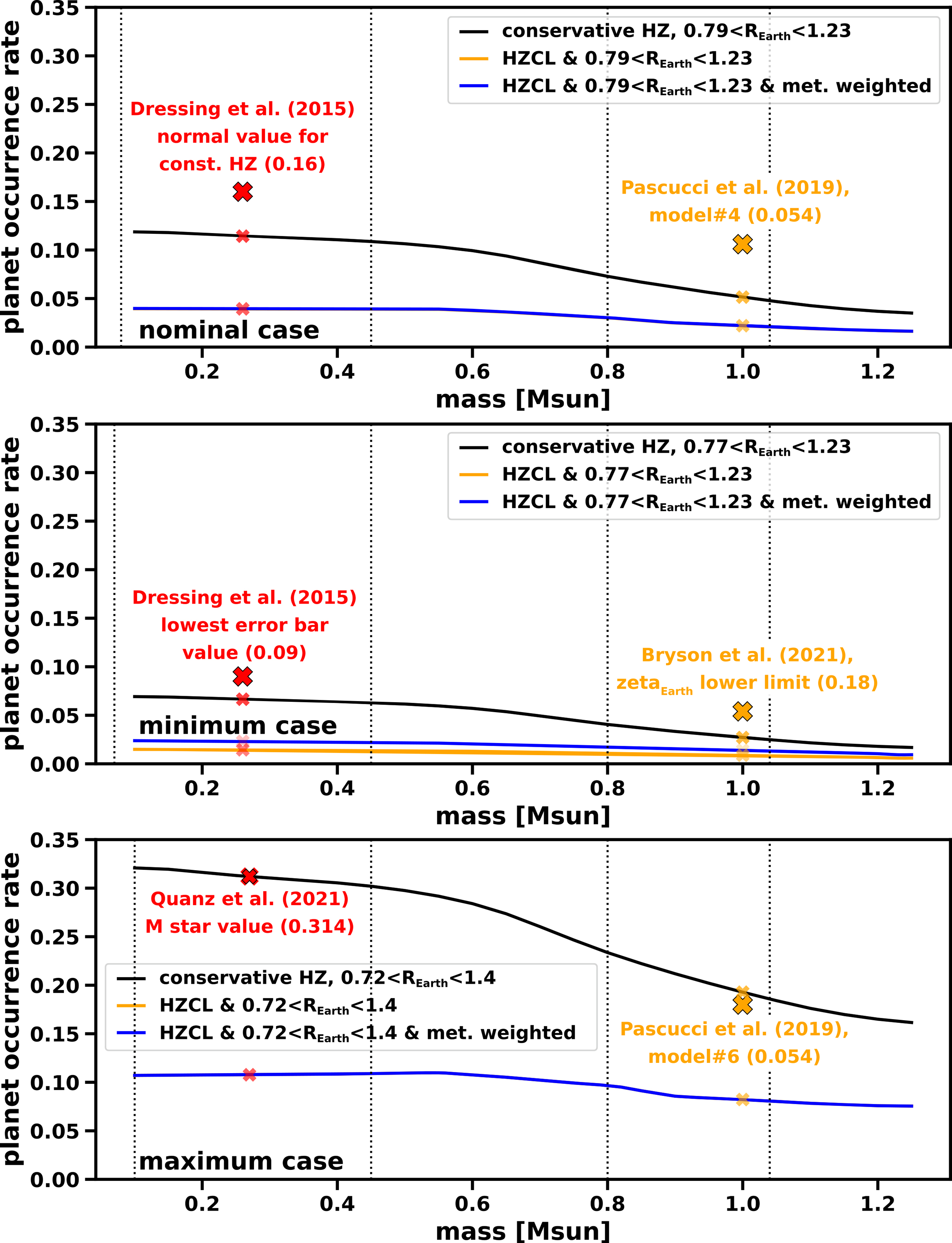
Planet occurrence rates for our nominal (upper), minimum (middle), and maximum (lower panel) cases for an N2-O2-dominated atmosphere with
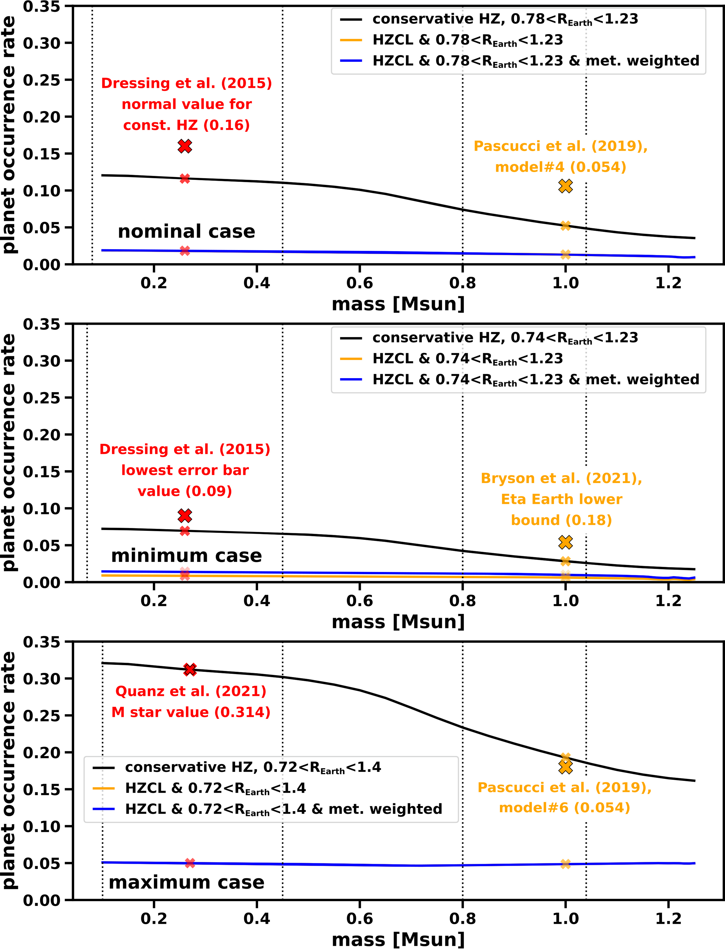
The same as Figure 23, but for an N2-O2-dominated atmosphere with
For an atmosphere with
All these values were scaled with the broken power law coefficients from model 4 of Pascucci et al. (2019). If we take the same broken power laws but with the coefficients published by Mulders et al. (2018), the rocky planet occurrence rate in the HZCL of a solar-like star will change slightly from
Another obvious factor that affects
If we apply these occurrence rates to the sample of stars,
For N2-O2-dominated atmospheres with
The requirement for having an appropriate planetary compositional and mineralogical setup,
Since our knowledge about exoplanet characteristics, their geophysical parameters, and statistics, as well as their relationship to the origin and evolution of life, is still at a basic level, the importance of only a few necessary requirements is at present quantifiable to some certain extent. In contrast, many are debated, or may not even be known yet. Within Sections 6.2 and 6.3, we therefore focus on the chosen few that can already be implemented via relatively reasonable and quantifiable scientific arguments, and which are further refinable, or potentially refutable, by future observations.
Further necessary requirements specifically feeding into
For
In this study, we highlight the caveat that it cannot be precisely answered at present whether an EH, and as a next step complex life, can also evolve on water worlds without any subaerial land, or even on subsurface-ocean worlds (which are excluded from our definition of EHs). A potential habitat fully covered by an ocean certainly provides different conditions than a world with subaerial land. However, future models and observations of exoplanets can give further insights and potentially correct and refine the parameter space of our study. Next, we therefore implement
The H2O requirement,
Calculating and implementing
For implementing
Tian and Ida (2015) calculated the loss of water via the well-known energy-limited escape formalism, a relatively simple prescription of thermal atmospheric escape that is limited by a star’s XUV luminosity (Salz et al., 2016; Watson et al., 1981), and which is known to often underestimate volatile loss for small and/or highly irradiated planets (Krenn et al., 2021; Kubyshkina et al., 2018). Kimura and Ikoma (2022), on the contrary, simulated atmospheric escape through a hydro-based approximation (HBA) equation found by Kubyshkina et al. (2018) through fitting a vast range of hydrodynamic upper atmosphere simulations. Both approaches are linearly dependent on the incident XUV flux from the host star, although the HBA approach can deviate from linear dependence for highly irradiated close-in planets where the atmospheric escape scales with
Tian and Ida (2015) provide results for stars with
Figure 2 in Tian and Ida (2015) provides a detailed breakdown of the final number of planets within certain water mass fractions. Since this figure only shows ratios in orders of magnitude, it is not entirely clear how many of the planets displayed fall within our range. For the G-type star we, therefore, take 74 out of 407 planets that are between a water mass fraction of
For K dwarfs with M
⋆ = 0.5
For M dwarfs with M
⋆ = 0.3
To further obtain occurrence rates of planets with the correct water mass fraction over the entire stellar mass spectrum, we simply assume that the occurrence rates between stars with stellar masses of
Figure 25 shows the derived occurrence rates for our nominal, maximum, and minimum cases as a function of stellar mass. The different crosses display the planet frequencies with appropriate water mass fractions based on the results of Tian and Ida (2015), Simpson (2017), and Kimura and Ikoma (2022), as described above. The dotted lines display occurrence rates derived from linear correlations with stellar
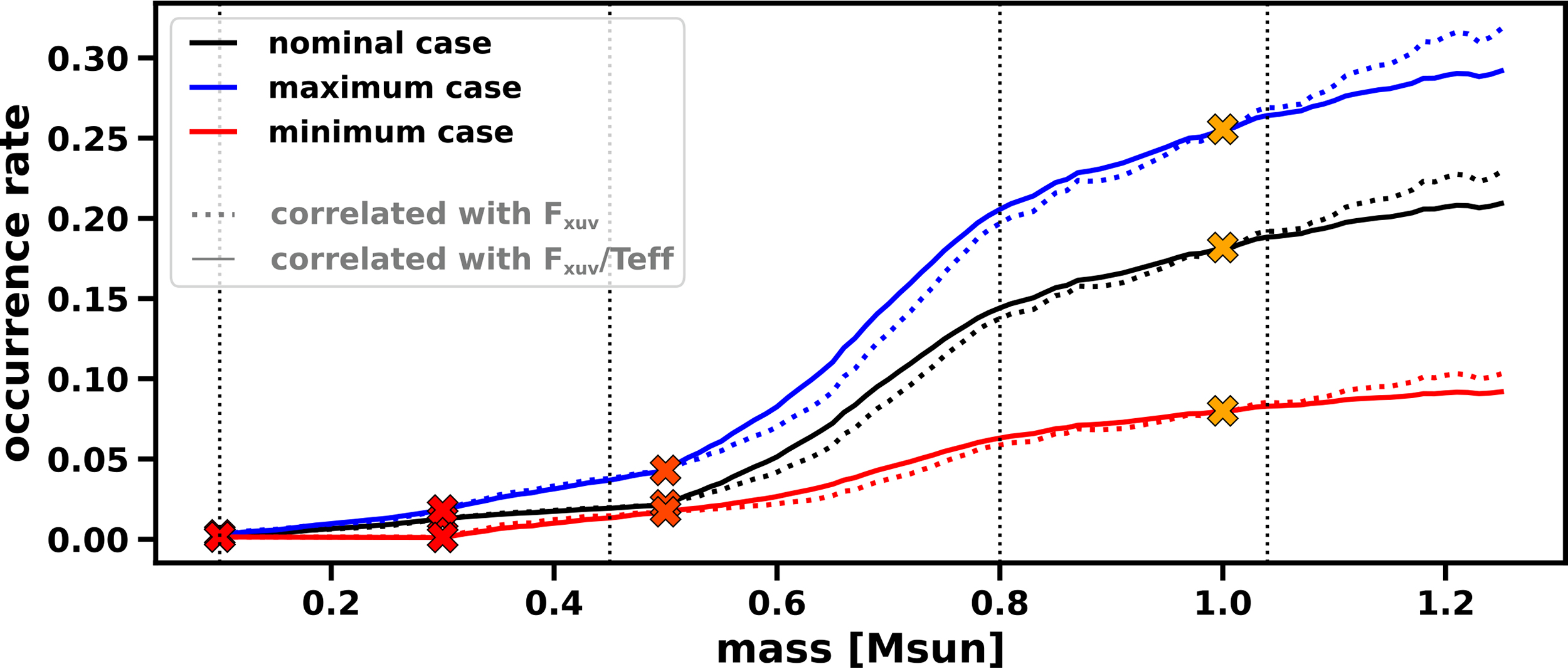
The frequency of planets with an appropriate water mass fraction as a function of stellar mass for our nominal (black), maximum (blue), and minimum (red) cases. The dotted lines show occurrence rates for which we assumed a simple linear correlation with
For our nominal case with
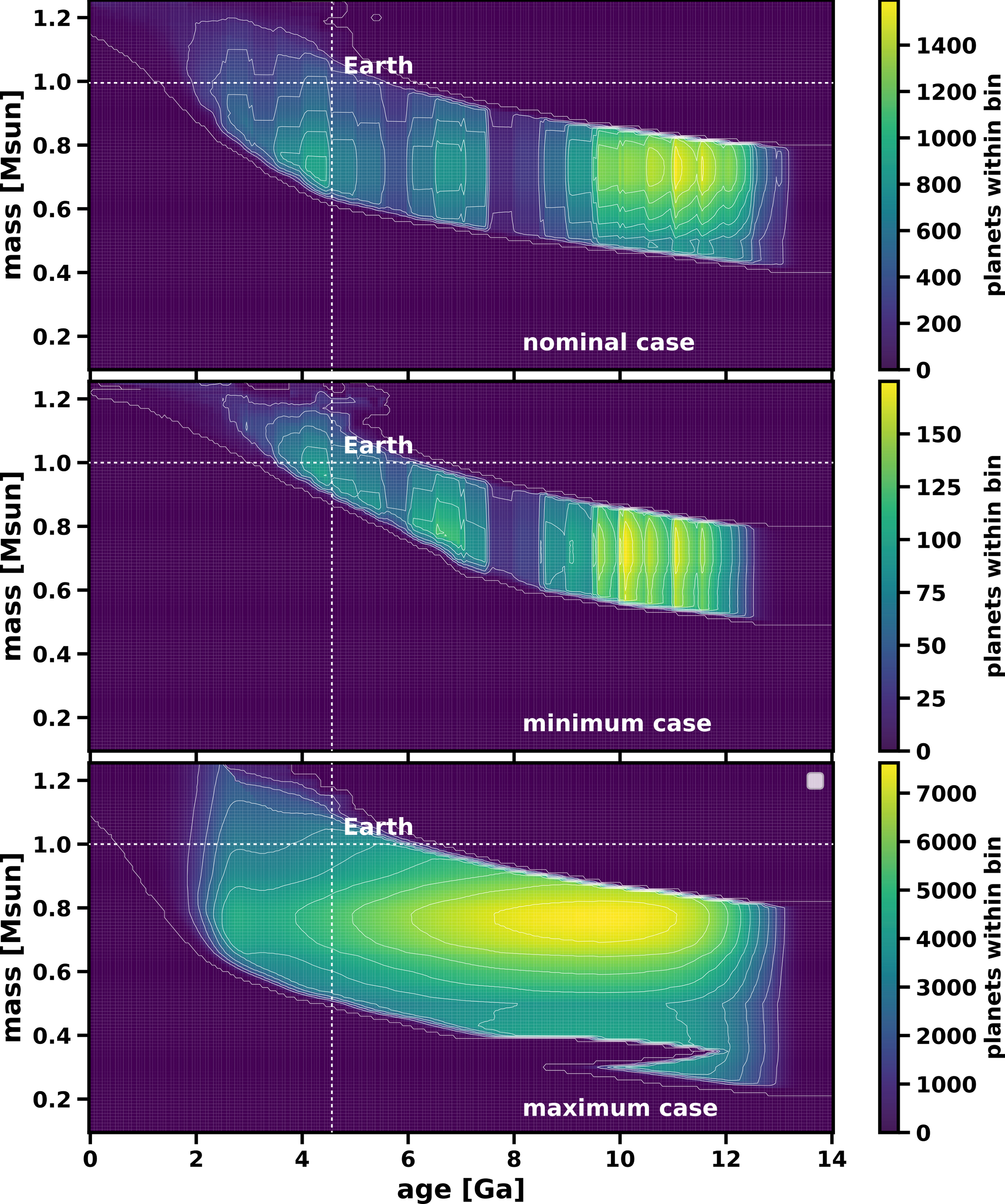
The distribution of remaining planets with the right amount of water that can in principal host an N2-O2-dominated atmosphere with
So, by only including
Several necessary parameters feed into the required long-term environmental stability term,
We know that the importance of a large moon for the evolution of an Earth-like biosphere may not be entirely clear. However, we include it into our model (i) since its potential prevalence can be discussed and estimated, and (ii) to illustrate one of the potential requirements feeding into
The large moon requirement,
Implementing
For implementing the large moon requirement, we start with occurrence rate simulations based on solar-like stars. As outlined in the appended Section 4.2, Elser et al. (2011) simulated the frequency of large moons around Earth-like planets. We implement their results for our nominal, minimum, and maximum cases for stars with a stellar mass of
For M dwarfs, we can apply the results by Martínez-Rodríguez et al. (2019), who specifically studied the orbital stability of moons around the by-then-known planets in the HZ of M stars. As these authors have calculated, 4 out of 33 planets are in principle capable of providing stable conditions for timescales longer than the Hubble time, t 0. To obtain an estimate on the occurrence rate of large satellites around M dwarfs, we can simply multiply the fraction of stable moons found by Martínez-Rodríguez et al. (2019) with the fraction of systems that may form a large moon in the first place, as simulated by Elser et al. (2011). This implicitly assumes that the general formation of large satellites around M dwarfs occurs with a frequency similar to that of G stars and that each of these moons indeed allows habitable conditions over large timescales (a potential overestimate, as explained above). The obtained value will then be applied to the mean stellar mass of the M-type spectral class.
To obtain a continuous frequency distribution over the entire range of stellar masses, we correlate the frequency of large moons with the host planet’s Hill radius,
Figure 27 shows the occurrence rate distributions for our nominal (black), maximum (blue), and minimum cases (red), and for our corresponding atmospheric scenarios with
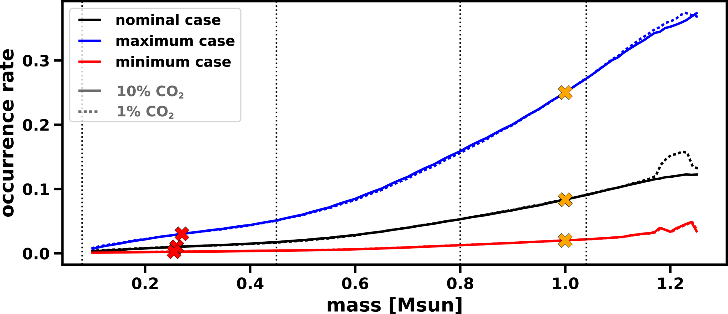
The frequency of planets with a large moon as a function of stellar mass for our nominal (black), maximum (blue), and minimum (red) cases, and for the corresponding atmospheric scenarios with
To put our occurrence rates into further context, we can compare them with some of the lunar survival rates calculated by Dobos et al. (2021), even though there are not many HZ planets currently known to have a radius comparable with the Earth. However, the planet Kepler-186f with a radius of
Based on our derived distribution, we get a total range of
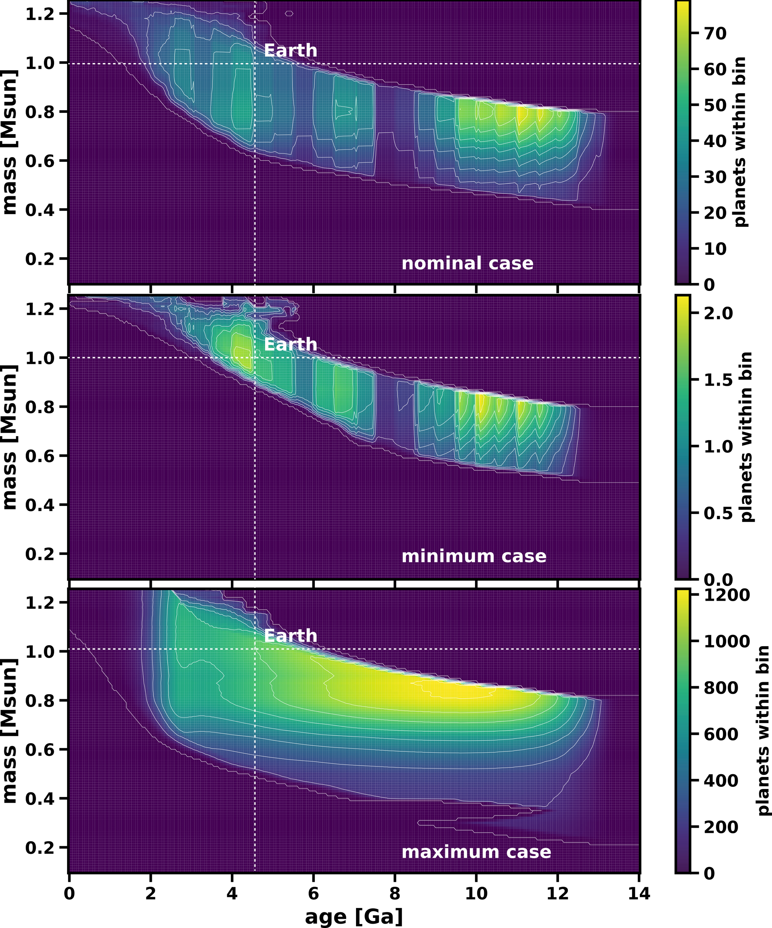
The distribution of planets with N2-O2-dominated atmosphere containing
By including the large moon requirement, however,
Our scientific knowledge about the planetary conditions to be met for a system to develop into an EH is relatively poor. Accordingly, only three requirements feeding into
The frequency of rocky exoplanets in the HZCL
By scaling different estimates of
The appropriate water mass fraction
Based on different geophysical and planet formation studies, we find that
The importance of a large moon
Several arguments point to the potential importance of a large moon to allow for the evolution of EHs. However, to account for the possibility that habitable worlds may also emerge by resolving the arguments listed in appended Section D.1 without the need of a large satellite, we find that
Interestingly, all three implemented planetary requirements show broadly similar importance, as can also be seen in Table 4 and Figure 29. The upper panel of the latter shows the requirements implemented into
The Effect of the Necessary Requirements onto
The Effect of the Necessary Requirements onto
For an N2-O2-dominated atmosphere with a maximum of 10% CO2.
Same, but with a maximum of 1% CO2.
All planets, except for “suitable stars.”

Same as Figure 20 but for necessary requirements only related to
Whereas for our two atmospheric cases, the maximum frequency of suitable stars was found to be
Combining both,
Our maximum values for
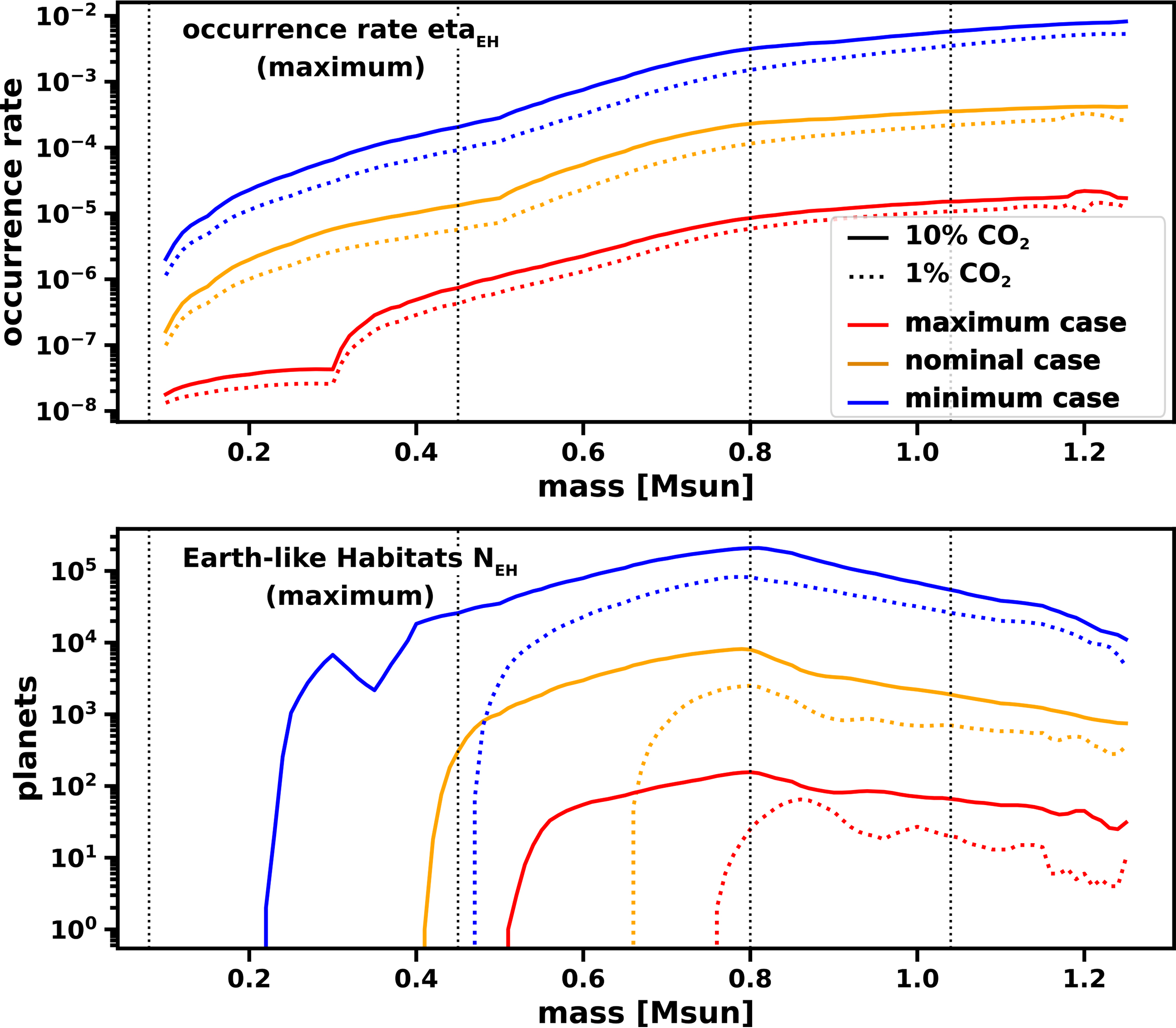
Maximum values for
The largest number of EHs can be expected to exist in the K-type spectral class for all our cases. This is in good agreement with a study by Cuntz and Guinan (2016), who also found early-type K dwarfs to be the most promising targets for finding advanced life-forms by implementing the frequency of stellar types, the speed of stellar evolution, the size of the respective HZs, and the stellar radiation environment into their model. It also fits well with the analysis by Lingam and Loeb (2021), who found that different models of stellar habitability, for example, the maximum habitability interval, the propensity of a planet to host life based on major evolutionary events, and the likelihood of attaining post-great oxygenation event (GOE) oxygen levels, converge toward early K-type stars as the most viable targets for life.
In our model, a stellar mass of
Figure 31 further illustrates the distribution of
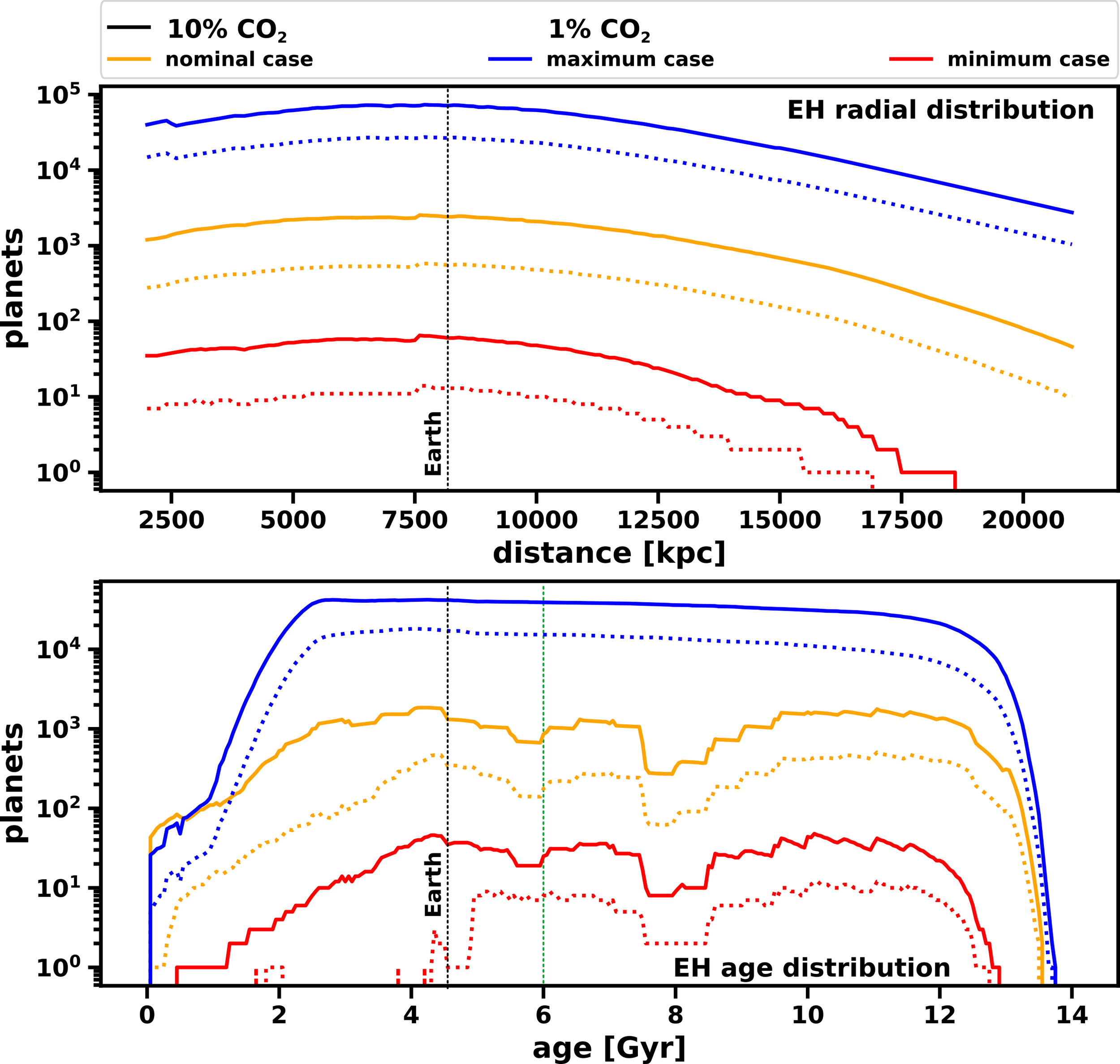
Maximum numbers for
As can further be seen in the lower panel of Figure 31, most of the planets in our final sample are older than the Earth (see also Fig. 28). Many of these planets may already be geologically inactive and, therefore, likely uninhabitable. This again illustrates that the actual number of EHs within the galactic disk will be significantly lower than our maximum number. To illustrate this point, for atmospheres with
Finally, Figure 32 illustrates the sample of remaining planets as a function of birth age and spectral class for both of our atmospheric cases, whereas Table 5 gives the fractions of stars within the different spectral classes. The relative distribution between the spectral classes changed significantly from the initial distribution of

The birth age of all remaining planets within our sample by spectral class for an N2-O2-dominated atmosphere with a maximum of 10% CO2 (upper) and 1% CO2 (lower panel), respectively. Here, the different colors illustrate the various spectral classes (with black as the sum of all) and solid, dashed, and dotted lines illustrating nominal, maximum, and minimum cases. The vertical dashed line indicates the approximate age at which geological activity on planets cosmochemically similar to the Earth may cease (see text).
The Distribution of Potentially Habitable Planets Within the Different Stellar Spectral Classes
The first two rows (i.e.,initial
As discussed earlier and as illustrated in Figure 32, any remaining planets around M dwarfs, and even many around K and to a lesser extent G dwarfs, belong to old stellar systems. If we, consequently, remove any stars that are older than 6 Gyr by assuming that bodies older than this age have, on average, stopped being geologically active, the distribution of remaining planets further shifts toward higher mass stars (see also Table 5). For N2-O2-dominated atmospheres with
This also indicates that most of the planets theoretically suitable to evolve into EHs may be relatively short-lived due to the limited lifetime of F stars. Whether enough time remains on such planets to reach atmospheric oxygenation (see Section E.2.3) similar in abundance to the Earth’s for allowing the subsequent evolution of complex life remains unanswered by our study. However, if a lifetime comparable with that of today’s Earth turns out to be crucial (see Catling et al., 2005), complex life could actually be favored around late-type G and early-type K dwarfs, potentially making Earth special among all habitable planets, but not atypical among EHs able to host complex life.
Our final outcome for
Compared with
, EHs will be rare
We find relatively low values for the fraction of stars,
In addition, we emphasize that
Our derived numbers are a plausible maximum range
As already pointed in Section 3.2, we first caution to take our values from the minimum and maximum cases as realistic maximum numbers, since we always implemented minimum and maximum values from the scientific literature for our minimum and maximum cases, respectively. It can therefore be assumed that the actual maximum number of EHs is closer to our nominal case. We also remind the reader that our minimum and maximum cases are, strictly speaking, the minimum and maximum among all the possible maximum values, thereby displaying the variation on the maximum number of EHs. The “true” minimum of
That said, the reason why our estimate is a plausible upper bound for the prevalence of EHs in the galactic disk is simple. As already discussed, several necessary requirements feed into
For the sake of the argument, we can simply assume that the combined requirements of having long-term working carbon–silicate and nitrogen cycles have a prevalence among our remaining sample of planets of
This brief exercise illustrates that EHs might indeed be rare in the galaxy and that their actual number can be much lower than our maximum estimate, potentially by orders of magnitude. Such a reasoning is also illustrated by calculating the minimum mean occurrence rate that each of the requirements not implemented into our model can have for
Could
be an underestimate?
There are certain arguments and reasons for our maximum values to potentially underestimate EHs within the galactic disk, mostly based on the following two arguments:
Underestimated occurrence rates
We could theoretically underestimate the occurrence rate of one of our implemented requirements significantly, a possibility that cannot be excluded. It may, for instance, turn out that N2-O2-atmospheres are to a higher extent thermally stable than currently expected through several different studies. It may also turn out that the sterilizing effect of SNs is too conservative, if the evolution of complex life on other planets on average happens faster and/or any putative life-forms on these planets evolved a better resilience against harsh radiation environments compared with Earth. In addition, large moons could turn out to be nonessential for EHs to evolve with any argument in favor of their importance being resolved by other means. However, we tried to implement each requirement to the best of our scientific knowledge and attempted to cover a wide parameter range for each factor as found in the scientific literature. If we took the much narrower range for the appropriate water mass fraction from Stern and Gerya (2024) for our nominal case with
As another example, if it were to turn out that Earth-like atmospheres are thermally stable for much higher XUV fluxes than currently expected, as suggested by one recent study (Nakayama et al., 2022, also see the discussion in Section A.2), it would only marginally change our results. Apart from the XUV requirement, several other implemented requirements significantly affect planets around low-mass stars. So, even if we assume that such atmospheres are still stable for XUV fluxes as high as 100F
So, even if Earth-like atmospheres were to be stable for higher XUV fluxes, they would likely still be unstable around M dwarfs due to nonthermal escape being highly detrimental. The nonthermal losses will even be further enhanced in such a case since the stable HZCL boundaries move closer to the star by increasing the XUV threshold (because the XUV threshold is reached earlier, the HZCL boundaries will be closer to the host star at this particular age, implying that the stellar wind ram pressure and hence nonthermal escape will be higher than at larger orbital distances).
Factors that may increase
Second, there could be factors that might actually increase the prevalence of EHs. Apart from some benefits that one or the other factor discussed in appended Section 5 may have, the most obvious example are EHs that form not on exoplanets but on exomoons. Exomoons, however, will only increase our results negligibly, if at all—and certainly far within any reasonable error bars—because of the following reasons.
First, any gas giant with an exomoon that could host an Earth-like atmosphere has to be within the HZCL as well. Fernandes et al. (2019), for instance, found the occurrence rate of giant planets between 1 and 20 Jupiter masses, M
These gas giants, however, would also need to have exomoons and these exomoons would have to be very large. Otherwise, any N2-O2-dominated atmosphere would not be stable around such a moon. If we put Titan today at the position of the Earth, its N2-dominated atmosphere would not be stable (see Sproß et al., 2021), even for the Earth’s presently low XUV surface flux, which is nonetheless ∼100 times higher compared with Saturn’s orbit at 10 AU. So, the mass of such an exomoon would have to be significantly higher than Titan’s, possibly comparable with the mass of the Earth. But how high might the occurrence rate of such exomoons be? These will be very rare and could potentially exist only around gas giants much more massive than Jupiter. They will logically have a frequency that is much lower than mentioned above.
But are such massive exomoons even possible? Canup and Ward (2006) found a common mass scaling of
It is not hard to see that Earth-mass or even Mars-mass exomoons in the HZCL of suitable stars will be exceedingly rare. And this does not even consider any potential additional habitability issues of exomoons around massive gas giants. These, for example, include the highly energetic particle environment within their extended magnetospheres through which such exomoons have to pass at least when orbiting through their tails (Heller and Zuluaga, 2013)—in case that their orbits are not entirely within the magnetosphere anyway. Tidal forces would also be critical for the habitability of exomoons around low-mass stars. As was found by Zollinger et al. (2017), no habitable moon would be possible for stellar masses of
Also, habitable planets around BDs and white dwarfs (Barnes and Heller, 2013), other potential environments to consider, are unlikely because of their dim and steadily decreasing HZs (Barnes and Heller, 2013; Lingam et al., 2020) and, at least in the case of white dwarfs, efficient tidal heating and high UV surface fluxes (Barnes and Heller, 2013). One should note, however, that a recent study by Becker et al. (2023) found specific scenarios for which tidal heating may keep a planet’s surface around a white dwarf above freezing for up to 10 Gyr. However, as the authors point out, they did not consider how tidal heating and the UV flux from the host dwarf might affect such planet’s atmosphere.
In this study, one could further note the hypothetical habitability of planets around neutron stars. To evaluate such habitability, Patruno and Kama (2017) calculated HZ boundaries and atmospheric escape for various neutron star environments and planetary masses. According to their estimates, super-Earths could retain their atmospheres for up to several hundred million years if their initial atmospheric mass fraction was a substantial part of the planet’s mass. If a moderately strong planetary magnetic field were additionally present and/or the pulsar winds were nonisotropic, habitable conditions would even be preserved for several billion years. To allow for temperatures above freezing, however, Patruno and Kama (2017) argue that the atmospheres of these planets will have to be heated via X-ray and gamma-ray radiation. For this to happen, the XUV surface fluxes in the respective HZs would have to reach values that are about six orders of magnitude higher than at today’s Earth orbit. Any atmosphere would therefore be lost significantly faster than estimated by Patruno and Kama (2017), who assumed hydrostatic atmospheres with no XUV-induced expansion at all. This can be regarded to be highly unrealistic. Moreover, planets around neutron stars would experience significant tidal heating and obliquity variations, the latter as much as
The movie Interstellar55 also spurred a whole bunch of scientific publications on whether planets around BHs can exist and even host life. Although these may indeed exist around stellar BHs and could potentially even form around SMBHs (Wada et al., 2019, 2021; Giang et al., 2022), the emergence of life, and specifically complex life, will be highly restrictive due to several astrophysical and relativistic reasons as discussed in several studies (Opatrný et al., 2017; Schnittman, 2019; Bakala et al., 2020; Iorio, 2020; Veysi, 2023). Even if life may evolve on some of these rare habitats though, it would be entirely different from EHs with very narrow timescales for evolution due to the relativistic phenomenon of time dilation (Veysi, 2023). Although habitats other than EHs may potentially exist, these will not increase our maximum number of EHs, as these are by definition no EHs. This is true for any other kind of hypothetical habitat.
EHs around M dwarfs could be exceedingly rare
As our results show, EHs around M dwarfs may only exist under very rare circumstances. Our model found cutoff masses of
Our lower stellar cutoff masses are in very good agreement with Lingam and Loeb (2021) and Cuntz and Guinan (2016), who both discuss lower stellar mass thresholds below which the existence of complex life becomes unlikely. For most of their investigated criteria, Lingam and Loeb (2021) observe a sharp decrease in their likelihood below a stellar mass range of
Our result that EHs around M dwarfs are exceedingly rare is also quite robust. Many crucial criteria disfavor M dwarfs as hosts for surficial life as we know it and there are several more crucial criteria than implemented into our model (see Section E). So, even if some requirements turned out to be less important, other important factors would remain. We discuss the implications of this reasoning on the falsifiability of our model further down below in Section 7.7.
Criteria disfavoring EHs at M dwarfs—potentially nonexhaustively—are as follows: The XUV surface flux in the HZCL of M dwarfs will remain high for billions of years (Birky et al., 2021; Engle, 2024; Fleming et al., 2020; Johnstone et al., 2021a; McDonald et al., 2019), thereby leading to thermal atmospheric escape and the loss of water (France et al., 2020; Johnstone et al., 2019a; Tian et al., 2008a; Tian and Ida, 2015; Tian, 2015; Van Looveren et al., 2024). High rates of flaring (Günther et al., 2020; Howard et al., 2019; Vida et al., 2019) will increase atmospheric escape (France et al., 2020) and potentially sterilize the surface (Howard et al., 2019; Tilley et al., 2019). However, it was also suggested to increase UV levels to allow prebiotic chemistry (Mullan and Bais, 2018)—a very thin line indeed between erosion and sterilization on the one hand and prebiotic chemistry on the other. The strong stellar winds in the HZCL (Garraffo et al., 2016) will lead to very high rates of nonthermal losses (Airapetian et al., 2017; Dong et al., 2020; France et al., 2020), in addition to thermal escape, even if a magnetosphere might be present (Garcia-Sage et al., 2017; Rodríguez-Mozos and Moya, 2019). Nonthermal losses alone can lead to a very fast loss of the atmosphere (Lichtenegger et al., 2010); taken both, thermal and nonthermal escape, together, even CO2-dominated atmospheres might not be stable around most low-mass M dwarfs. The strong and rapidly varying stellar magnetic field at the orbit of a rocky exoplanet around an M dwarf will lead to immense joule heating in the upper atmosphere comparable or even larger than the heating induced by the incident XUV surface flux, as was recently shown by Cohen et al. (2024). This process alone will likely be sufficient to completely erode a secondary atmosphere. The very slow decrease in stellar luminosity will lead to a strong shift of the HZCL so that planets initially within will later be outside (Ramirez and Kaltenegger, 2014). So, even if such planets finally end up in the HZCL, they might have already lost their atmosphere and water (Lammer et al., 2011; Luger and Barnes, 2015; Tian and Ida, 2015) or entered the Runaway Greenhouse state early-on (Ramirez and Kaltenegger, 2014). The probability of possessing an appropriate water mass fraction for simultaneously having surface water and subaerial land might be significantly lower than for planets around FGK stars (Kimura and Ikoma, 2022; Tian and Ida, 2015). These planets could completely desiccate due to the high water loss into space, end up as water worlds, or even with steam atmospheres (Marounina and Rogers, 2020). Planets around M dwarfs have a low chance of forming and keeping a large moon due to stronger tidal interaction with the host star (Martínez-Rodríguez et al., 2019; Piro, 2018; Tokadjian and Piro, 2020). For low-mass M dwarfs, it may even be impossible. However, tidal interaction with the host star could at least partially substitute for some of a large moon’s positive effects—but it could also overheat the planet, thereby rendering it uninhabitable (McIntyre, 2022). Induction heating around M dwarfs with strong magnetic fields could lead to extreme volcanism (Kislyakova et al., 2018; Kislyakova and Noack, 2020). This could be favorable for the carbon–silicate cycle. It could, however, also overheat the planet or desiccate it from all volatiles during the active phase of the host star. The same is true for flare-CME-induced interior heating, another relevant process recently discussed by Grayver et al. (2022). After the long, active phase of the host star decreases below the stability threshold level for N2-O2-dominated atmospheres, the planets may already be depleted by all volatiles and/or be geologically dead. Such planets cannot build up Earth-like atmospheres, thereby inhibiting the emergence of EHs. The UV flux availability will likely be too low to allow for substantial prebiotic chemistry (Buccino et al., 2006; Buccino et al., 2007). The chance for an origin of life might therefore be highly reduced. The effectiveness of photosynthesis might similarly be limited and the oxygenation time around M dwarfs will take too long for complex life to evolve (Lingam and Loeb, 2021). In general, the available total energy received at such planet over the entire Hubble time may likely be too low to allow for complex life (Haqq-Misra, 2019). However, flares could increase such energy, but this might be a double-edged sword. Abiotic buildup of O2 could reduce the chance for the origin of life and/or limit its early evolution due to oxidized conditions disfavoring the origin and evolution of early life as we know it (Lingam, 2020). It could further decrease the UV availability at a planet’s surface due to ozone formation. Photochemical conditions in the atmospheres of planets orbiting M dwarfs can lead to relatively high atmospheric levels of the highly toxic CO (Schwieterman et al., 2019a, 2019b), providing an additional obstacle for complex life (Schwieterman et al., 2019a). The same seems to be the case for ozone, as Cooke et al. (2024) found surface O3 concentrations to substantially surpass 40 ppb in several of their atmospheric simulations for Trappist-1e and Proxima Centauri b, with maximum concentrations reaching up to 2200 ppb—values lethal for life on Earth. Planets around M dwarfs might not receive enough reduced atmospheric compounds—an important source of prebiotic molecules—to kick-start prebiotic chemistry and the origin of life, as late comet and meteorite impacts will be highly reduced or even absent (Anslow et al., 2023; Lichtenberg and Clement, 2022). In general, asteroid belt analogs for the delivery of volatiles and prebiotic molecules may be rare around M dwarfs. But still, M dwarfs will suffer significantly more high-velocity impacts than planets around larger host stars, a substantial challenge for the evolution of complex life (Anslow et al., 2023). Planets around M dwarfs are likely tidally locked (Barnes, 2017). Warm climates can evolve at such worlds with low CO2 partial pressures as long as the planet is not too dry (Turbet et al., 2016). However, it remains to be seen whether EHs could indeed evolve on such planets.
The listed criteria further increase the likelihood of EHs being exceedingly rare around M dwarfs. Such rareness will also resolve the so-called red sky paradox as posited by Kipping (2021), in line with this author’s supposed “resolution IV,” which states that “M dwarfs have fewer habitable worlds.”
The highest rates of EHs
The highest probability to find EHs could be within the K-type spectral class, specifically around ∼0.8
The rate and distance of EHs in the solar neighborhood
By only considering G stars and the solar neighborhood, with a sphere of 0.5 kpc around the Sun, the occurrence rate of EHs will be higher than over both the entire stellar mass range and galactic disk. For this, we find occurrence rates of
We can also calculate the average minimum distance,
This behavior can be seen in Figure 33, which compares the average distance between EHs in the galactic disk,
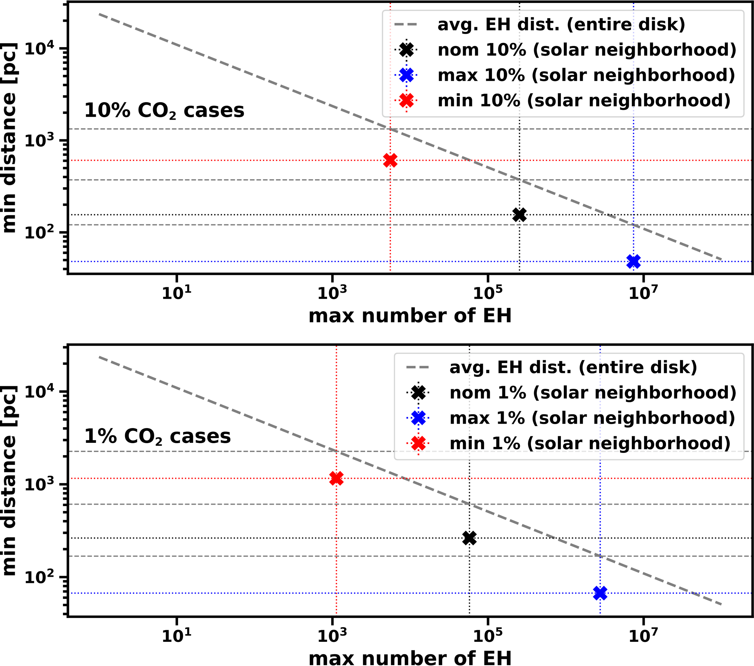
Upper panel: The minimum average distance,
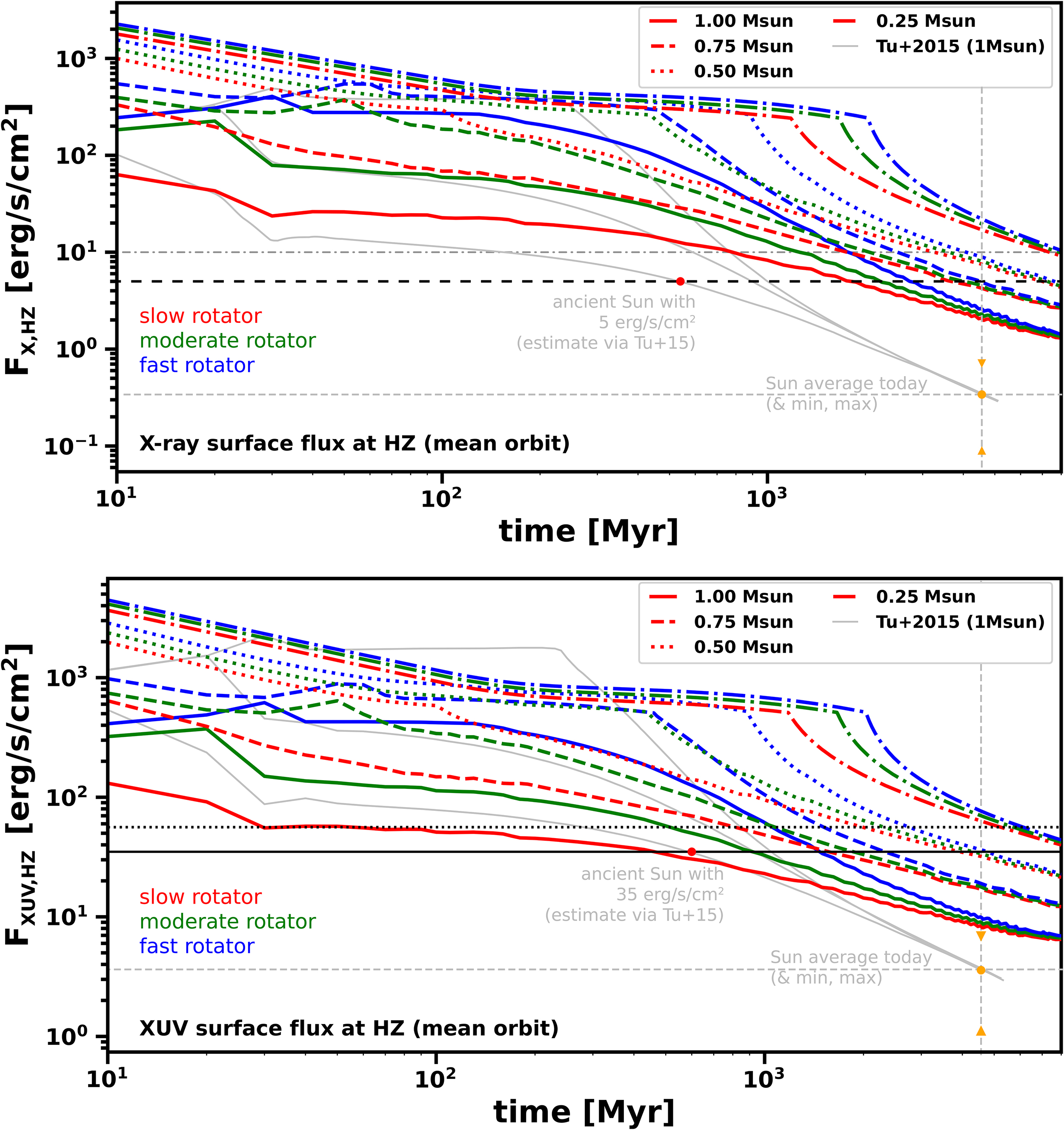
Upper panel: The evolution of the stellar X-ray surface flux,

Exobase altitudes for N2-atmospheres with different CO2 mixing ratios and for different X-ray surface fluxes,
As already discussed, some additional requirements will likely become scientifically quantifiable in the next decades. Current and future exoplanet missions are therefore highly important. With the ground-based facilities ELT and Thirty Meter Telescope, space missions JWST, Ariel, and PLATO, and their potential successors LIFE and the HWO, further criteria can be quantified to such an extent that these can be included in future assessments on the prevalence of EHs. Exoplanet atmosphere characterization might relatively soon be able to tell us, whether rocky exoplanets accrete relatively fast and mostly within the disk, and how many of them will host primordial atmospheres. This could also tell us something about the prevalence of working carbon–silicate and nitrogen cycles, possibly even about the frequency of life as we know it, by statistically characterizing the compositions of exoplanetary atmospheres. Upcoming missions will at some time be able to give us estimates on the occurrence rates of CO2-dominated and O2-rich atmospheres, planets without thick H2- and He-envelopes, and maybe even on N2-dominated atmospheres. Future missions such as PLATO (Rauer et al., 2014) will also refine our knowledge on
All these factors taken together will make our results testable in the relatively near future. Discovering scientific hints on
This also relates to our reasoning that EHs around M dwarfs are exceedingly rare. This conclusion implies that the search for signs of life at planets orbiting low-mass stars will likely return a lack of robust atmospheric biosignatures.56 This endeavor has already recently started to be partly on its way, most prominently with JWST, which can already perform detections of atmospheric molecules that are often assumed to be related to life such as O3, O2, CH4, and H2O. JWST can further give hints on whether or not a rocky exoplanet is hosting a secondary atmosphere. This was already tentatively illustrated for the rocky M dwarf planets Trappist-1b (Greene et al., 2023), Trappist-1c (Zieba et al., 2023),57 GJ 341b (Kirk et al., 2024), and LHS 475b (Lustig-Yaeger et al., 2023), whose observations are all consistent with having no or only very tenuous atmospheres.
It is hence worth pointing out that robust discoveries of biosignatures and/or N2-dominated atmospheres on rocky exoplanets in the HZCL of M dwarfs would serve as a means of falsifying our model’s predictions, thereby indicating that at least certain arguments within our model must be wrong. From a scientific point of view this is good, as it meets the Popperian standard of science.
Finally, our work can help guiding the design of next-generation telescopes, potentially beyond LIFE and HWO, in case our results will not be falsified by finding EHs in the solar neighborhood. Our average minimum distance,
Habitats other than EHs
Our study tells nothing about any habitats other than EHs, whether these may be subsurface ocean worlds or water worlds, Titan-like habitats, planets with a completely different biochemistry, or even worlds with anaerobic microbial life still able to evolve into EHs.
One may, however, simply extend our formulation to take account of other habitats, Ni
, that is,
By including hypothetical Titan-like habitats,
These and other potential habitats may be common in the galaxy, but our present study is completely agnostic about them and whether life evolves on these more exotic worlds. In this study, we should hence note that, while the existence of an EH may already imply the presence of aerobic denitrifying microbes, anaerobic anammox species, and/or any other microbes that recycle N2 back into the atmosphere, any estimated numbers, for example,
Our result that EHs are relatively rare also implies that the emergence of (aerobic) CETI in the galaxy—the main target of SETI (Drake, 1961, 1965; Tarter, 2001)—will likely be rare as well. In fact, it will be significantly rarer than EHs per se since additional requirements must be met for ETIs to evolve, specifically, if these should be technologically advanced species that intend to send radio messages into space and who are able to listen to what others are sending. That no definitive signals from ETIs were hence detected by SETI comes by relatively little surprise.
However, that the emergence of aerobic ETIs will be rare due to a small number of viable sites for their initial evolution does not necessarily mean that once an ETI indeed evolved, it, or its postbiological successors, could not become more widespread in the Milky Way than complex life itself (Lingam and Loeb, 2019b; Wright et al., 2022). While the latter will evolve within a specific biosphere with a finite lifetime, a technological civilization emerging from an EH can outlive its initial biosphere (Balbi and Ćirković, 2021). In principle, it can even colonize planets other than EHs, and hence spread efficiently58 throughout the galactic disk and even beyond (Walters et al., 1980). One should keep such uncertainties and caveats in mind for the following discussion.
That said, if (i) EHs indeed are rare, but (ii) some other aerobic ETIs nevertheless exist in today’s galaxy, intentionally sending signals into space to communicate with whoever might be out there, can be an unwise action to take. In this case, the potential rareness of EHs implies that the Earth itself, with its N2-O2-dominated atmosphere, is a very valuable resource for any aerobic ETI currently existing in the Milky Way. This is even more true if these ETIs indeed possess the relevant technology to spread from their original EH into interstellar space and toward other valuable planets. It would thus come by no surprise if technologically advanced species would have a certain interest in our “Pale Blue Dot.” This reasoning would be strongly supported if some of the controversially discussed unidentified aerial phenomena (UAPs)59 had actually originated on an EH other than ours, as our results would then not only indicate that these objects must have traveled a considerable distance, but could also explain the actual reason for their visit: the Earth as a rare and valuable resource. Even if these ETIs were benevolent, however, first contact could have negative impact on humanity (Schetsche and Anton, 2018).
Intentionally signaling that we, and the Earth specifically, are actually here, as is the aim of METI (Baum et al., 2011; Haqq-Misra et al., 2013; Vakoch, 2011, 2016) and as was recently proposed by Jiang et al. (2022), can therefore add some kind of unnecessary, diffuse, and incalculable danger that, at least with our present knowledge, cannot be properly assessed and may therefore neither be neglected nor evoked. In this study, it is important to note that radio leakage and other techno- and atmospheric signatures can in principle be detected from close by ETIs, but an intentional, strong, and focused signal such as the Arecibo message in 1974 will reach much farther into space (Haqq-Misra et al., 2013).
Sending messages into space must be discussed broadly, specifically by also considering the argument that EHs might be rare. Even though some of the past METI initiatives have been more transient than other terrestrial radio sources (Sullivan et al., 1978; Baum et al., 2011; Haqq-Misra et al., 2013), this was not the case for the Arecibo message and will not be the case for certain future attempts. It should also be emphasized that justifying METI by pointing to the detectability of unintended radio leaks from Earth appears to be a relatively poor argument for intentional signaling to ETIs, as this can also be seen as an argument for minimizing the leakage of technosignatures in the future. Baum et al. (2011) stressed that intentional messages to ETIs should not contain specific biological information about humans, as we do not know whether these will be received by a malicious ETI. These authors further argue that we should avoid being recognized as an expanding civilization to minimize the possibility of being perceived as a threat. This argument is further strengthened by our finding that EHs are rare. The destruction of one of these rare habitats indeed leaves quite an alarming impression on any intelligent observer.
But how many separately emerged and evolved aerobic ETIs could indeed exist in the Milky Way at present? For some simple estimate, we can easily extend our formulation, that is,
Here,
If we assume
This rather simple estimate does not include any other potential requirements needed to properly estimate
If one wants to calculate the maximum number of planets inhabited by ETIs or visited by self-replicating probes (Bracewell, 1960; Freitas, 1980; Tipler, 1980) instead of the maximum number of separately emerged and evolved (aerobic) ETIs, however, this formalism would have to be extended for covering interstellar travel within the galaxy, by including an additional settling factor S (Lingam and Loeb, 2021), as was already suggested to be added to the Drake equation (Walters et al., 1980; Brin, 1983). In addition, the above formulation does not include nonbiological, AI-based civilizations that descended from biological, aerobic ETIs or any other intelligent extraterrestrials (biological and nonbiological) that originated on habitats other than EHs. For this, we can simply extend Equation 34 as follows:
Moreover, it is, in turn, very likely that SETI observations will have to wait quite a while to detect technological emissions from ETIs in the galaxy, if they exist at all. This conclusion is well supported by Grimaldi (2023), who, based on Bayesian reasoning, finds “optimistic waiting times” for such a signal to be 60–1800 years with a probability of 50%. If EHs, and hence ETIs, are very rare, these waiting times may indeed be quite optimistic.
Finally, we emphasize that the Principle of Mediocrity, or more specifically, the Copernican Principle of Mediocrity (see Gott, 1993; Ćirković, 2012; Scharf, 2014; Westby and Conselice, 2020) in the sense of the Earth not being special and (complex or even intelligent) life consequently being common in the Universe (Sagan, 1994), cannot be regarded to be valid on the specific level of individual planets, as was recently also pointed out by Balbi and Lingam (2023). The Earth is certainly not special in the sense of being central to the galaxy or even the Universe. However, the occurrence rate of rocky exoplanets,
It is therefore also not surprising that our maximum estimate on ETIs in the galactic disk is much lower than the one provided by Westby and Conselice (2020), who defined and applied a specific form of the Copernican Principle called the “astrobiological Copernican Principle.” They define it as follows: Any sufficiently Earth-like planet (i.e., “suitable planet”) in the HZ of a “suitable star” will form (intelligent) life over a time frame of ∼5 Gyr in a similar fashion than the Earth. Westby and Conselice (2020) further define “suitable star” as any star with an age greater than 5 Gyr and a sufficiently high metallicity to allow for the evolution of advanced biology and ETIs. The term “suitable planet” further refers to any rocky exoplanet within the HZs of such stars. Based on this astrobiological Copernican Principle, Westby and Conselice (2020) derive the following modification of the Drake equation, that is,
Westby and Conselice (2020) further split the astrobiological Copernican Principle into a “Weak” and “Strong” scenario, of which the first one presumes that intelligent life needs at least 5 Gyr to evolve, while the second assumes that intelligent life must form between 4.5 and 5.5 Gyr. If we take their “Strong” scenario with
These exemplary discrepancies clearly illustrate that not every rocky planet in the HZ(CL) can simply be considered habitable. Such an assumption can even be wrong by orders of magnitude. If planetary parameters are very similar to each other, then it is not of great importance whether we live on this or on any other planet that fulfills certain parameters. In this tautological sense, the Copernican Principle logically holds. However, there are these specific requirements that shall be met for making a planet habitable for life as we know it and only a small fraction of planets will meet these criteria. In such a stricter sense, the Copernican Principle cannot be applied and the Earth is indeed special or even rare (at least in relation to the total number of stars and the planets orbiting in their HZCLs) and, based on such principle, it is a fallacy to assume that (complex) life is common in the Universe, even if one sets the unknown frequency of life originating to be equal to unity.
One could, however, argue for some kind of combined Anthropic-Copernican Principle that states that certain special conditions have to be met for life as we know it to evolve. As long as these conditions can evolve at some place, the Copernican Principle suffices, and life as we know it might be common on such worlds (see also Gott, 1993). However, these combined conditions will be rare on a galactic scale, and in that sense the Anthropic Principle (Carter, 1983) holds as well. It might thus not be a coincidence that we live somewhere in the middle of the galaxy on an Earth-mass planet below an Earth-like atmosphere that orbits within the HZCL of a mid-aged, anomalously weakly active G-type star that has surface water, subaerial land, and a large moon on which intelligent species can set foot on for embarking onto their journey into space.
In this study, we provide a comprehensive overview on all the input parameters that feed into our different simulations (i.e., into nominal, minima, and maxima cases for N2-O2-dominated atmospheres with
Input Parameters for Simulating the Number of Stars in the Disk,
, and the Resulting Stellar Properties
Input Parameters for Simulating the Number of Stars in the Disk,
Note that parameters that are the same for several cases are only listed once per row and distributed over the respective cases they refer to.
Note that these values are equivalent with
Derived in Section 4.3.
IMF, initial mass function; SFR, star formation rate.
Input Parameters Feeding into Simulating
Note that parameters that are the same for several cases are only listed once per row and distributed over the respective cases they refer to.
Model 4 by Gowanlock et al. (2011), taken from the upper panel of their Fig. 6.
Model 2 by Gowanlock et al. (2011), again from the upper panel of their Fig. 6.
From here onward, we only consider stars within our chosen mass range, that is,
From here onward “fraction” denotes the fraction of stars that remain after implementing the specific requirement onto the remaining sample of stars.
From here onward “cumulative fraction” denotes the fraction of stars that remain from the initial sample of disk stars as are found within the entire mass range.
Metallicity evolution normalized to fit present-day (Fe/H)-value of Hayden et al. (2015) for each galactic spatial bin in our model.
For the outer disk (r >7.5 kpc), we took the metallicity evolution of Snaith et al. (2015) “with dilution.”
To calculate the percentage of stars per galactic spatial bin with a certain (Fe/H) value to be above
Runaway greenhouse limit as calculated through Kopparapu et al. (2014).
Runaway greenhouse limit calculated through Kopparapu et al. (2013).
Outer HZCL boundary for p
Outer HZCL boundary for p
In units of effective stellar surface flux at Earth.
Runaway greenhouse limit from Kopparapu et al. (2014).
Runaway greenhouse limit from Leconte et al. (2013b).
Runaway greenhouse limit from Kopparapu et al. (2013).
This equals the maximum number of stars suitable for EHs in our model, that is,
This, finally, equals the maximum value for
EHs, Earth-like habitats; HZ, habitable zone; HZCL, habitable zone for complex life; XUV, X-ray and extreme ultraviolet.
Input Parameters Feeding into Simulating
Note that parameters that are the same for several cases are only listed once per row and distributed over the respective cases they refer to.
The initial values for the used radius and orbital period ranges can be found in the cited studies
Occurrence rate always taken for a stellar mass of 1.0M⊕.
From Pascucci et al. (2019), model 4.
From Bryson et al. (2021), lower bound.
From Pascucci et al. (2019), model 6.
Occurrence rate always taken for the mean stellar mass of the M dwarf spectral class in the respective case (values are different for the different cases and the corresponding masses are written in brackets).
From Dressing and Charbonneau (2013).
From Quanz et al. (2022).
From Dressing and Charbonneau (2013), lower value of the uncertainty range.
The respective orbital period ranges are taken from the HZCL boundaries as defined in Table 7, whereas the radius ranges are displayed in this table.
The derived
The power law used for scaling
The power law reduces to
Planetary minimum radius used for scaling
Calculated with the relationship used for the exoplanet yield estimates of space missions Habitable Exoplanet Observatory, Large UV Optical Infrared Surveyor, and Large Interferometer for Exoplanets, that is,
This radius corresponds to a minimum planetary mass of 0.3M⊕, see again Section 6.1.1 and Zink and Hansen (2019).
Planetary maximum radius for scaling
The derived transition radius between rocky and neptunian planets according to Chen and Kipping (2017), see also Section 6.1.1.
Based on a “conservative interpretation” (Gaudi et al., 2020) of the derived transition between rocky and neptunian planets from Rogers (2015).
For the same average stellar masses as for the M star
Stellar variable through which the displayed occurrence rates for FGK (i.e., for 1M⊕) and M mean stellar masses are linearly scaled to all stellar masses (see Eq. 26 and discussion in Sect. 6.2.1).
Factor through which
Equivalent with the mean occurrence rate,
Input Parameters Feeding into Simulating
Note that parameters that are the same for several cases are only listed once per row and distributed over the respective cases they refer to.
The appropriate planetary water mass fraction for simultaneously hosting subaerial land and ocean was always assumed to be
From Tian and Ida (2015), planets in Fig. 2 between water mass fractions of
From Tian and Ida (2015), planets in Fig. 2 between water mass fractions of
From Simpson (2017), fraction not entirely covered by oceans from the right panel of their Fig. 5 (solid line).
From Kimura and Ikoma (2022) for
From Kimura and Ikoma (2022) for
Stellar variable through which the displayed occurrence rates for the specific predefined G, K, and M stellar masses are linearly scaled to all stellar masses.
From Elser et al. (2011), mean value.
From Elser et al. (2011), maximum value.
From Elser et al. (2011), minimum value.
Same mean M star masses as for the planet occurrence rate, that is, 0.26, 0.27, and 0.26
Fraction of stable moons around M stars (i.e., 4/33 moons) from Martínez-Rodríguez et al. (2019) multiplied with minimum, maximum, and mean values from Elser et al. (2011) for G stars (i.e., our corresponding occurrence rates for G stars).
Variable through which the displayed occurrence rates for G and M mean stellar masses are linearly scaled to all stellar masses, in this case, the planetary Hill radius (see Equations 27 and 28 and discussion in Section 6.3.1).
This equals the final maximum number of EHs found in our model, that is,
This equals the final maximum occurrence rate,
This finally equals the maximum occurrence rate
In addition, Tables 10 and 11 provide similar information than the smaller Table 5 but list the distribution of remaining stars/planets within the different stellar spectral classes for each of the implemented requirements, and additionally provide numbers for stars that are both older than 6 Gyr and younger than 4 Gyr to account for (i) an Earth-like oxygenation time of Gyr and (ii) the potential cessation of geological activity at cosmochemically Earth-like planets. Table 10 lists these values for
The Distribution of Potentially Habitable Planets/Stars That Remain After Implementing the Respective Requirement as a Function of Different Stellar Spectral Classes (for a Maximum of 10% CO2) a
The maximum 10% CO2 scenario is identical to the maximum 1% CO2 for all requirements before the upper limit.
The Distribution of Potentially Habitable Planets/Stars That Remain After Implementing the Respective Requirement as a Function of Different Stellar Spectral Classes (for a Maximum of 1% CO2) a
The maximum 1% CO2 scenario is identical to the maximum 10% CO2 for all requirements before the upper limit.
Scaled with the broken power law of model 4 by Pascucci et al. (2019).
For solar-like star with
Radius scaled with surface flux
A mean radius of 0.72
In this study, we applied our formulation to calculate the maximum number of EHs in the galactic disk, as introduced in Paper I. Our methodological and scientifically quantifiable approach shows that, in agreement with the rare Earth hypotheses (Ward and Brownlee, 2000), EHs in the galaxy should indeed be rare by deriving maximum numbers of
Our results have profound additional implications, as the likely rareness of EHs further implies complex aerobic and intelligent life to be rarer still. Since a breathable atmosphere will present a very valuable resource for any aerobic ETIs, they might show a certain interest in our planet. Intentionally sending messages into space should therefore be performed with high caution. We also point out that our study is agnostic about life originating on hypothetical habitats other than EHs. Any more exotic habitats (e.g., subsurface ocean worlds) could significantly outnumber planets with Earth-like atmospheres, at least in principle. Finally, we argue that the Copernican Principle of Mediocrity cannot be valid in the sense of the Earth and consequently complex life being common in the galaxy. Certain requirements must be met to allow for the existence of EHs and only a small fraction of planets indeed meet such criteria. It is therefore unscientific to deduce complex aerobic life to be common in the Universe, at least based on the Copernican Principle. Instead, we argue, at maximum, for a combined Anthropic-Copernican Principle stating that life as we know it may be common, as long as certain criteria are met to allow for its existence. Extremophiles, anaerobic and simple aerobic life-forms, however, could be more common.
In a future study, we plan to assess the maximum number of EHs on a statistical basis, and to implement further criteria into our model. We therefore plan to include volatile budgets, volcanic degassing, and possible geological activity timescales, as these can refine our results. Studying the evolution of habitability throughout galactic history is another research topic that we like to address in the future.
Footnotes
Acknowledgments
M.S. acknowledges the FWF project FWF-ESPRIT D-1522P33620 and also thanks D. Kubyshkina for fruitful discussions. We also thank four anonymous referees for their thoughtful and valuable comments and suggestions that helped to improve the article significantly.
Appendix 1
Appendix 2
Appendix 3
Appendix 4
Appendix 5
Associate Editor: Charley Lineweaver