Given a simple noun such as apple, and a question such as “Is it edible?,” what processes take place in the human brain? More specifically, given the stimulus, what are the interactions between (groups of) neurons (also known as functional connectivity) and how can we automatically infer those interactions, given measurements of the brain activity? Furthermore, how does this connectivity differ across different human subjects?
In this work, we show that this problem, even though originating from the field of neuroscience, can benefit from big data techniques; we present a simple, novel good-enough brain model, or GeBM in short, and a novel algorithm Sparse-SysId, which are able to effectively model the dynamics of the neuron interactions and infer the functional connectivity. Moreover, GeBM is able to simulate basic psychological phenomena such as habituation and priming (whose definition we provide in the main text).
We evaluate GeBM by using real brain data. GeBM produces brain activity patterns that are strikingly similar to the real ones, where the inferred functional connectivity is able to provide neuroscientific insights toward a better understanding of the way that neurons interact with each other, as well as detect regularities and outliers in multisubject brain activity measurements.
1. Introduction
Consider human subject “Alice,” who is reading a typed noun (e.g., apple) and has to answer a simple yes/no question (e.g., Can you eat it?). How do different parts of Alice's brain communicate during this task? This type of communication is formally defined as functional connectivity of the human brain and is an active field of research in neuroscience. Coming up with a comprehensive model that captures the dynamics of the functional connectivity is of paramount importance. Achieving that will effectively provide a better understanding of how the human brain works and can have a great impact both on machine and human learning. In this work, we tackle the above problem in a scenario where multiple human subjects are shown simple nouns and answer a set of questions for each noun, and we record their brain activity using magentoencephalography (MEG).
Although this might seem like a problem that is of sole interest to the field of neuroscience, in fact, it can also benefit from a big data approach. For the human subjects, what we essentially have is a set of MEG sensors recording a time series of the magnetic activity of their brain, and our ultimate goal is to infer a (hidden) underlying network between different regions of their brain. Effectively, we are dealing with a problem of the broad family of network discovery, which is an active field of big data research; for instance, in Verscheure et al.1 the authors induce a communication network between VoIP users through time-series analysis, while in Sadilek et al.2 the authors infer a friendship network between Twitter users by using various signals of user behavior.
“THUS, IT IS IMPORTANT TO VIEW THIS PROBLEM THROUGH A BIG DATA ANALYTICS LENS, AND THIS ARTICLE CONSTITUTES A STEP IN THIS DIRECTION.”
Besides the nature of the problem itself, the data involved in our problem call for big data techniques: For the human subjects, an experiment involves recording their brain activity for all combinations of nouns and questions, which results in a big number of data points that need to be processed, summarized, and analyzed; as the task becomes more complicated (e.g., the subject has to read an entire sentence, or a book instead of a single typed noun, or even look at a picture), the data volume and complexity explode. In addition to that, different measurement techniques have complementary strengths (e.g., MEG has fine time granularity but poor spatial resolution, and conversely fMRI has very high, 1 mm spatial resolution but poor temporal resolution), and we would like to collect and exploit all potential benefits from all techniques, a factor that significantly increases the size of the problem; for instance, even for a small number of human subjects, all measurements span hundreds of gigabytes. Thus, it is important to view this problem through a big data analytics lens, and this article constitutes a step in this direction.
Our approach: Discovering the multibillion connections among the tens of billions3,4 of neurons would be the holy grail, and clearly outside the current scientific and technological capabilities. How close can we approach this ideal? We propose to use a good-enough approach, and try to explain as much as we can by assuming a small, manageable count of neuron-regions and their interconnections, and trying to guess the connectivity from the available MEG data. In more detail, we propose to formulate the problem as “system identification” from control theory, and we develop novel algorithms to find sparse solutions.
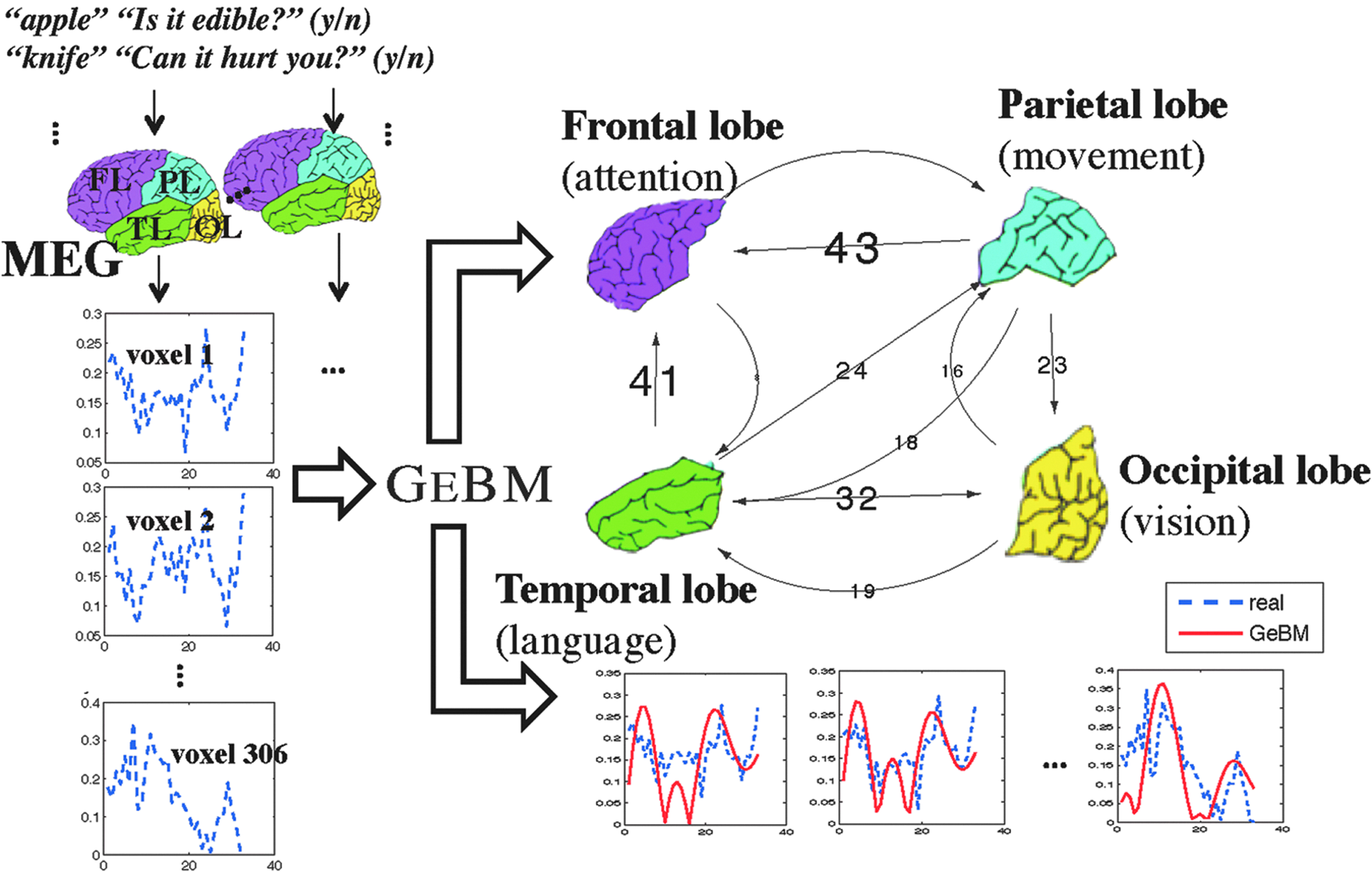
We show that our good-enough approach is a very good first step, leading to a tractable, yet effective model (the good-enough brain model, or GeBM), that can answer the above questions. Figure 1 gives the high-level overview: At the bottom right, the blue, dashed-line time sequences correspond to measured brain activity; the red lines correspond to the guess of our GeBM model. Notice the qualitative goodness of fit. At the top right, the arrows indicate interaction between brain regions that our analysis learned, with the weight being the strength of interaction. Thus we see that the vision cortex (“occipital lobe”) is well connected to the language-processing part (“temporal lobe”), which agrees with neuroscience, since all our experiments involved typed words.
Big picture: Our good-enough brain model (GeBM) estimates the hidden functional connectivity (top right, weighted arrows indicating number of inferred connections), when given multiple human subjects (left) that respond to yes/no questions (e.g., edible?) for typed words (e.g., apple). (Bottom right) GeBM also produces brain activity (in solid red) that matches reality (in dashed blue).
Our contributions are as follows:
• Novel analytical model and algorithm: We propose the GeBM model [see section 3, and Eq. (2)–(3)]. We also introduce Sparse-SysId, a novel sparse system-identification algorithm (see section 3).
• Effectiveness: Our model can explain psychological phenomena, such as habituation and priming (see section 5.4); it also gives results that agree with experts' intuition (see section 5.1).
• Multisubject analysis: Our Sparse-SysId, applied on nine human subjects (section 5.2), showed that (a) eight of them had very consistent brain-connectivity patterns while (b) the outlier was due to exogenous factors (excessive road-traffic noise during the outlier's experiment).
• Cross-disciplinary connections: Our GeBM highlights connections between multiple, mostly disparate areas: (1) neuroscience, (2) control theory & system identification, and (3) psychology. Additionally, we provide insights on the relation of GeBM to recurrent neural networks, a field that is gaining increasing popularity among big data techniques, especially with the rise of deep learning, pointing out ways that both can benefit from each other.
Reproducibility: Our implementation is publicly available online.5 Due to privacy reasons, we are not able to release the MEG data, however, in the online version of the code we include the synthetic benchmarks, as well as the simulation of psychological phenomena using GeBM.
The present manuscript is an extension of our work that appeared in the ACM SIGKDD Conference on Knowledge Discovery and Data Mining (ACM KDD) 2014 conference5. In addition to Papalexakis et al.5 in this manuscript, we provide further cross-disciplinary connections of our work to other fields (and more specifically to recurrent neural networks), provide intuitive explanations behind the key concepts introduced in the original article, as well as emphasize the practical applications of our work.
2. Problem Definition
As mentioned earlier, our goal is to infer the brain connectivity, given measurements of brain activity on multiple yes/no tasks of multiple subjects. We define as yes/no task the experiment in which the subject is given a yes/no question (such as “Is it edible?” and “is it alive?”), and a typed English word (such as apple or chair), and has to decide the answer.
Throughout the entire process, we attach m sensors that record brain activity of a human subject. Here we are using magnetoencephalography (MEG) data, although our GeBM model could be applied to other types of measurement (fMRI, etc). In section 5 we provide a more formal definition of the measurement technique.
Thus, in a given experiment, at every time-tick t we have m measurements, which we arrange in an m×1 vector y(t). Additionally, we represent the stimulus (e.g., apple) and the task (e.g., Is it edible?) in a time-dependent vector s(t), by using feature representation of the stimuli; a detailed description of how the stimulus vector is formed can be found in section 5. For the rest of the article, we shall use interchangeably the terms sensor, voxel, and neuron-region.
“FIRST AND FOREMOST, WE ARE INTERESTED IN UNDERSTANDING HOW THE BRAIN WORKS, GIVEN A SINGLE SUBJECT.”
First and foremost, we are interested in understanding how the brain works, given a single subject. Informally, we have the following:
Informal Problem 1. Given:The input stimulus; and a sequence of m×T brain activity measurements for the m voxels, for all timeticks\documentclass{aastex}\usepackage{amsbsy}\usepackage{amsfonts}\usepackage{amssymb}\usepackage{bm}\usepackage{mathrsfs}\usepackage{pifont}\usepackage{stmaryrd}\usepackage{textcomp}\usepackage{portland, xspace}\usepackage{amsmath, amsxtra}\pagestyle{empty}\DeclareMathSizes{10}{9}{7}{6}\begin{document}
$$t = 1 \cdots T$$
\end{document}
Estimate:The functional connectivity of the brain, that is, the strength and direction of interaction, between pairs of the m voxels, such that
1. we understand how the brain-regions collaborate, and
2. we can effectively simulate brain activity.
After solving the above problem, we are also interested in doing cross-subject analysis to find commonalities (and deviations) in a group of several human subjects.
For the particular experimental setting, prior work6 has only considered transformations from the space of noun features to the voxel space and vice versa, as well as word-concept specific prediction based on estimating the covariance between the voxels.7
Next we formalize the problems, we show some straightforward (but preliminary) solutions, and finally we give the proposed model GeBM, and the estimation algorithm.
3. Problem Formulation and Proposed Method
There are two over-arching assumptions in our design:
• Linearity: Linear models, however simplifying, are a good “first order approximation” of the functional connectivity we seek to capture.
• Stationarity: The connectivity of the brain does not change, at least for the time-scales of our experiments.
The above assumptions might sound very simplifying; however, this work is a first step in this direction, and our linear, time-invariant model proves to be “good-enough” for the task at hand. Nonlinear/sigmoid models are a natural direction for future work, and so is the study of neuroplasticity, where the connectivity changes.
We must note that however simple GeBM is, there are simpler approaches that seem more natural at first, which do not perform well. Such an approach, which we call Model0, is presented in the next subsection, before the introduction of GeBM.
3.1. First (unsuccessful) approach: Model0
Since our informal problem definition does not strictly define the brain regions whose connectivity we are seeking to identify, a natural first step is to assume that each MEG voxel (e.g., region measured by an MEG sensor) is such a brain region.
Given the linearity and static-connectivity assumptions above, we may postulate that the m×1 brain activity vector y(t+1) depends linearly on the activities of the previous time-tick y(t), and, of course, the input stimulus, that is, the s×1 vector s(t).
Formally, in the absence of input stimulus, we expect that
\documentclass{aastex}\usepackage{amsbsy}\usepackage{amsfonts}\usepackage{amssymb}\usepackage{bm}\usepackage{mathrsfs}\usepackage{pifont}\usepackage{stmaryrd}\usepackage{textcomp}\usepackage{portland, xspace}\usepackage{amsmath, amsxtra}\pagestyle{empty}\DeclareMathSizes{10}{9}{7}{6}\begin{document}
\begin{align*}\textbf{y} ( t + 1 ) = \textbf{Ay} ( t )\end{align*}
\end{document}
where A is the m×m connectivity matrix of the m brain regions. Including the (linear) influence of the input stimulus s(t), we reach the Model0:
\documentclass{aastex}\usepackage{amsbsy}\usepackage{amsfonts}\usepackage{amssymb}\usepackage{bm}\usepackage{mathrsfs}\usepackage{pifont}\usepackage{stmaryrd}\usepackage{textcomp}\usepackage{portland, xspace}\usepackage{amsmath, amsxtra}\pagestyle{empty}\DeclareMathSizes{10}{9}{7}{6}\begin{document}
\begin{align*}\textbf{y} ( t + 1 ) = \textbf{A}_{[ m \times m ]} \times \textbf{y} ( t ) + \textbf{B}_{[ m \times s ]} \times \textbf{s} ( t ) \tag{1}\end{align*}
\end{document}
The B[m×s] matrix shows how the s input signals affect the m brain regions.
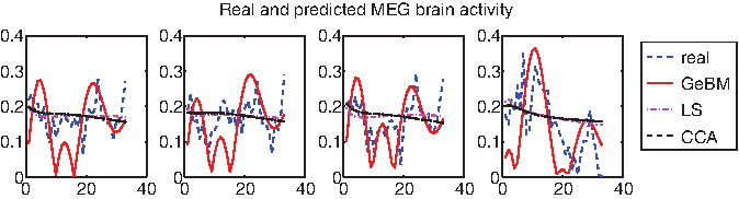
Papelexakis et al.5 we shows how we can solve for this model using least squares (LS) and canonical correlation analysis (CCA)8 However intuitive, the formulation of Model0 turns out to be rather ineffective in capturing the temporal dynamics of the recorded brain activity. As an example of its failure to model brain activity successfully, Figure 2 shows the real brain activity and predicted activity for a particular voxel. The solutions fail to match the trends and oscillations.
Model0 fails: True brain activity (dotted blue) and the model estimate (pink and black, resp., for the least squares and for the CCA variation).
The conclusion of this subsection is that we need a more sophisticated yet parsimonious model, which leads us to GeBM, as described next.
3.2. Proposed approach: GeBM
Before we introduce our proposed model, we should introduce our notation, which is succinctly shown in Table 1. Formulating the problem as Model0 does not meet the requirements for our desired solution. However, we have not exhausted the space of possible formulations that live within our set of simplifying assumptions. In this section, we describe GeBM, our proposed approach that, under the assumptions that we have already made in section 2, is able to meet our requirements remarkably well.
Table of Symbols
Symbol
Definition
n
number of hidden neuron-regions
m
number of MEG sensors/voxels we observe (306)
s
number of input signals (40 questions)
T
time-ticks of each experiment (340 ticks, of 5 msec each)
x(t)
vector of neuron activities at time t
y(t)
vector of voxel activities at time t
s(t)
vector of input-sensor activities at time t
A[n×n]
connectivity matrix between neurons (or neuron regions)
C[m×n]
summarization matrix (neurons to voxels)
B[n×s]
perception matrix (sensors to neurons)
Av
connectivity matrix between voxels
Real
real part of a complex number
Imag
imaginary part of a complex number
A†
Moore-Penrose pseudoinverse of A
MEG, magentoencephalography.
In order to come up with a more accurate model, it is useful to look more carefully at the actual system that we are attempting to model. In particular, the brain activity vector y that we observe is simply the collection of values recorded by the m sensors, placed on a person's scalp. In Model0, we attempt to model the dynamics of the sensor measurements directly. However, by doing so, we are directing our attention to an observable proxy of the process that we are trying to estimate (i.e., the functional connectivity). Instead, it is more beneficial to model the direct outcome of that process. Ideally, we would like to capture the dynamics of the internal state of the person's brain, which, in turn, causes the effect that we are measuring with our MEG sensors.
Let us assume that there are n hidden (hyper-)regions of the brain, which interact with each other, causing the activity that we observe in y. We denote the vector of the hidden brain activity as x of size n×1. Then, by using the same idea as in Model0, we may formulate the temporal evolution of the hidden brain activity as:
\documentclass{aastex}\usepackage{amsbsy}\usepackage{amsfonts}\usepackage{amssymb}\usepackage{bm}\usepackage{mathrsfs}\usepackage{pifont}\usepackage{stmaryrd}\usepackage{textcomp}\usepackage{portland, xspace}\usepackage{amsmath, amsxtra}\pagestyle{empty}\DeclareMathSizes{10}{9}{7}{6}\begin{document}
\begin{align*}\textbf{x} ( t + 1 ) = \textbf{A}_{[ n \times n ]} \times \textbf{x} ( t ) + \textbf{B}_{[ n \times s ]} \times \textbf{s} ( t )\end{align*}
\end{document}
A subtle issue that we have yet to address is the fact that x is not observed, and we have no means of measuring it. We propose to resolve this issue by modeling the measurement procedure itself, that is, model the transformation of a hidden brain activity vector to its observed counterpart. We assume that this transformation is linear, thus we are able to write
\documentclass{aastex}\usepackage{amsbsy}\usepackage{amsfonts}\usepackage{amssymb}\usepackage{bm}\usepackage{mathrsfs}\usepackage{pifont}\usepackage{stmaryrd}\usepackage{textcomp}\usepackage{portland, xspace}\usepackage{amsmath, amsxtra}\pagestyle{empty}\DeclareMathSizes{10}{9}{7}{6}\begin{document}
\begin{align*}\textbf{y} ( t ) = \textbf{C}_{[ m \times n ]} \textbf{x} ( t )\end{align*}
\end{document}
Putting everything together, we end up with the following set of equations, which constitute our proposed model GeBM:
\documentclass{aastex}\usepackage{amsbsy}\usepackage{amsfonts}\usepackage{amssymb}\usepackage{bm}\usepackage{mathrsfs}\usepackage{pifont}\usepackage{stmaryrd}\usepackage{textcomp}\usepackage{portland, xspace}\usepackage{amsmath, amsxtra}\pagestyle{empty}\DeclareMathSizes{10}{9}{7}{6}\begin{document}
\begin{align*}\textbf{x} ( t + 1 ) = \textbf{A}_{[ n \times n ]}
\times \textbf{x} ( t ) + \textbf{B}_{[ n \times s ]} \times
\textbf{s} ( t ) \tag {2}\end{align*}
\end{document}\documentclass{aastex}\usepackage{amsbsy}\usepackage{amsfonts}\usepackage{amssymb}\usepackage{bm}\usepackage{mathrsfs}\usepackage{pifont}\usepackage{stmaryrd}\usepackage{textcomp}\usepackage{portland, xspace}\usepackage{amsmath, amsxtra}\pagestyle{empty}\DeclareMathSizes{10}{9}{7}{6}\begin{document}
\begin{align*}\textbf{y} ( t ) = \textbf{C}_{[ m \times n ]} \times
\textbf{x} ( t ) \tag {3}\end{align*}
\end{document}
“WE REQUIRE THAT OUR MODEL'S MATRICES ARE SPARSE; ONLY FEW SENSORS MEASURE A SPECIFIC BRAIN REGION.”
The key concepts behind GeBM are:
• (Latent) Connectivity matrix: We assume that there are n regions, each containing 1 or more neurons, and they are connected with an n×n adjacency matrix A[n×n]. We only observe m voxels, each containing multiple regions, and we record the activity (eg., magnetic activity) in each of them; this is the total activity in the constituent regions.
• Measurement matrix: Matrix C[m×n] is an m×n matrix, with ci,j=1 if voxel i contains region j.
• Perception matrix: Matrix B[n×s] shows the influence of each sensor to each neuron region. The input is denoted as s, with s input signals.
• Sparsity: We require that our model's matrices are sparse; only few sensors measure a specific brain region. Additionally, the interactions between regions should not form a complete graph, and finally, the perception matrix should map only few activated sensors to neuron regions at any given time.
An interesting aspect of our proposed model GeBM is that if we ignore the notion of the summarization, that is, matrix C=I, then our model is reduced to the simple model Model0. In other words, GeBM contains Model0 as a special case. This observation demonstrates the importance of hidden states in GeBM.
A pictorial representation of GeBM is shown in Figure 3. Starting from left to right, we have the triangle-shaped nodes; these nodes represent the sensors of the human subject, which capture the stimulus s(t). For instance, these sensors could correspond at a high level to different visual sensors that map the stimulus to the internal, hidden neuron regions; the mapping between the human sensor nodes to the latent brain regions is encoded in matrix B. The hidden neuron regions are denoted by black circles, and the connections between them comprise matrix A, which is effectively the functional connectivity of these latent regions. Finally, the latent region activity x(t) is measured by the MEG sensors, which are denoted by black squares in Figure. 3; this measurement procedure is encoded in matrix C.
Sketch of GeBM
3.3. Algorithm
Our solution is inspired by control theory, and more specifically by a subfield of control theory, called system identification. We refer the interested reader to the appendix of our KDD article,5 and references therein, for an overview of traditional system identification. However, the matrices we obtain through this process are usually dense, counter to GeBM's specifications. We, thus, need to refine the solution until we obtain the desired level of sparsity. In the next few lines, we show why this sparsification has to be done carefully, and we present our approach.
Crucial to GeBM's behavior is the spectrum of its matrices; in other words, any operation that we apply to any of GeBM's matrices needs to preserve the eigenvalue profile (for matrix A) or the singular values (for matrices B and C). Alterations thereof may lead GeBM to instabilities. From a control theoretic and stability perspective, we are mostly interested in the eigenvalues of A, since they drive the behavior of the system. Thus, in our experiments, we heavily rely on assessing how well we estimate these eigenvalues.
As a reminder to the reader, here we provide a short explanation why eigenvalues are crucial. Say we focus on one of the eigenvalues λ of our matrix A. If λ is real and positive, then the response of the system (associated with λ) will increase exponentially. Conversely, if λ is real and negative, the respective response will decay exponentially. Finally, if λ is complex, then the response of the system will be some type of oscillation, whose frequency and trend (decaying, increasing, or constant) depends on the actual values of the real and the imaginary parts. The response of the system is, thus, a mixture of the responses that pertain to each eigenvalue. Say that by transforming our system's matrices, we force a complex eigenvalue to become real; this will alter the response of the system severely, since a component that was oscillating will now be either decaying or increasing exponentially, after the transformation.
In Sparse-SysId, we propose a fast greedy sparsification scheme. Iteratively, for all three matrices, we delete small values while maintaining the spectrum within \documentclass{aastex}\usepackage{amsbsy}\usepackage{amsfonts}\usepackage{amssymb}\usepackage{bm}\usepackage{mathrsfs}\usepackage{pifont}\usepackage{stmaryrd}\usepackage{textcomp}\usepackage{portland, xspace}\usepackage{amsmath, amsxtra}\pagestyle{empty}\DeclareMathSizes{10}{9}{7}{6}\begin{document}
$$\epsilon$$
\end{document} from the one obtained through system identification. Additionally, for A, we also do not allow eigenvalues to switch from complex to real and vice versa. This scheme works very well in practice, providing very sparse matrices, while respecting their spectrum. Doing so is important, because eigenvalues determine the dynamical behavior of our model. In Algorithm 1, we provide an outline of the algorithm.
Sparse-SysId: Sparse System Identification of GeBM
Input: Training data in the form \documentclass{aastex}\usepackage{amsbsy}\usepackage{amsfonts}\usepackage{amssymb}\usepackage{bm}\usepackage{mathrsfs}\usepackage{pifont}\usepackage{stmaryrd}\usepackage{textcomp}\usepackage{portland, xspace}\usepackage{amsmath, amsxtra}\pagestyle{empty}\DeclareMathSizes{10}{9}{7}{6}\begin{document}
$$\{\textbf{y} ( t ) , \textbf{s} ( t ) \} _{t = 1}^{T}$$
\end{document}, number of hidden states n.
Output:GeBM matrices A (hidden connectivity matrix), B (perception matrix), C (measurement matrix), and Av (voxel-to-voxel matrix).
1: {A(0),B(0),C(0)}=SysId\documentclass{aastex}\usepackage{amsbsy}\usepackage{amsfonts}\usepackage{amssymb}\usepackage{bm}\usepackage{mathrsfs}\usepackage{pifont}\usepackage{stmaryrd}\usepackage{textcomp}\usepackage{portland, xspace}\usepackage{amsmath, amsxtra}\pagestyle{empty}\DeclareMathSizes{10}{9}{7}{6}\begin{document}
$$\left( \{\textbf{y} ( t ) , \textbf{s} ( t ) \} _{t = 1}^{T} , n \right)$$
\end{document}
2: A=EigenSparsify(A(0))
3: B=SingularSparsify(B(0))
4: C=SingularSparsify(C(0))
5: Av=CAC†
3.4. Obtaining the voxel-to-voxel connectivity
So far, GeBM, as we have described it, is able to give us the hidden functional connectivity and the measurement matrix, but does not directly offer the voxel-to-voxel connectivity, unlike Model0, which models it explicitly. However, this is by no means a weakness of GeBM, since there is a simple way to obtain the voxel-to-voxel connectivity (henceforth referred to as Av) from GeBM's matrices. We highlight the importance of Av, since this matrix essentially maps abstract latent brain areas to physical brain regions.
EigenSparsify: Eigenvalue Preserving Sparsification of System Matrix A.
Input: Square matrix A(0).
Output: Sparsified matrix A.
1: λ(0)=Eigenvalues(A(0))
2: Initialize \documentclass{aastex}\usepackage{amsbsy}\usepackage{amsfonts}\usepackage{amssymb}\usepackage{bm}\usepackage{mathrsfs}\usepackage{pifont}\usepackage{stmaryrd}\usepackage{textcomp}\usepackage{portland, xspace}\usepackage{amsmath, amsxtra}\pagestyle{empty}\DeclareMathSizes{10}{9}{7}{6}\begin{document}
$$\textbf{d}_R^{( 0 )} = \textbf{0} , \textbf{d}_I^{( 0 )} = \textbf{0}$$
\end{document}. Vector \documentclass{aastex}\usepackage{amsbsy}\usepackage{amsfonts}\usepackage{amssymb}\usepackage{bm}\usepackage{mathrsfs}\usepackage{pifont}\usepackage{stmaryrd}\usepackage{textcomp}\usepackage{portland, xspace}\usepackage{amsmath, amsxtra}\pagestyle{empty}\DeclareMathSizes{10}{9}{7}{6}\begin{document}
$$\textbf{d}_R^{( i )}$$
\end{document} holds the element-wise difference of the real part of the eigenvalues of A(i). Similarly for \documentclass{aastex}\usepackage{amsbsy}\usepackage{amsfonts}\usepackage{amssymb}\usepackage{bm}\usepackage{mathrsfs}\usepackage{pifont}\usepackage{stmaryrd}\usepackage{textcomp}\usepackage{portland, xspace}\usepackage{amsmath, amsxtra}\pagestyle{empty}\DeclareMathSizes{10}{9}{7}{6}\begin{document}
$$\textbf{d}_I^{( i )}$$
\end{document} and the imaginary part.
3: Set vector c as a boolean vector that indicates whether the j-th eigenvalue in λ(0) is complex or not. One way to do it is to evaluate element-wise the following boolean expression: c=(Imag (λ(0))≠0).
4: Initialize i=0
5: while\documentclass{aastex}\usepackage{amsbsy}\usepackage{amsfonts}\usepackage{amssymb}\usepackage{bm}\usepackage{mathrsfs}\usepackage{pifont}\usepackage{stmaryrd}\usepackage{textcomp}\usepackage{portland, xspace}\usepackage{amsmath, amsxtra}\pagestyle{empty}\DeclareMathSizes{10}{9}{7}{6}\begin{document}
$$\textbf{d}_R^{( i )} \le \epsilon$$
\end{document}and\documentclass{aastex}\usepackage{amsbsy}\usepackage{amsfonts}\usepackage{amssymb}\usepackage{bm}\usepackage{mathrsfs}\usepackage{pifont}\usepackage{stmaryrd}\usepackage{textcomp}\usepackage{portland, xspace}\usepackage{amsmath, amsxtra}\pagestyle{empty}\DeclareMathSizes{10}{9}{7}{6}\begin{document}
$$\textbf{d}_I^{( i )} \le \epsilon$$
\end{document}and (Imag (λ(i))≠0)== c do
8: Set \documentclass{aastex}\usepackage{amsbsy}\usepackage{amsfonts}\usepackage{amssymb}\usepackage{bm}\usepackage{mathrsfs}\usepackage{pifont}\usepackage{stmaryrd}\usepackage{textcomp}\usepackage{portland, xspace}\usepackage{amsmath, amsxtra}\pagestyle{empty}\DeclareMathSizes{10}{9}{7}{6}\begin{document}
$$\textbf{A}^{( i )} ( v_i^* , v_j^* ) = 0$$
\end{document}
9: λ(i)=Eigenvalues(A(i))
10: \documentclass{aastex}\usepackage{amsbsy}\usepackage{amsfonts}\usepackage{amssymb}\usepackage{bm}\usepackage{mathrsfs}\usepackage{pifont}\usepackage{stmaryrd}\usepackage{textcomp}\usepackage{portland, xspace}\usepackage{amsmath, amsxtra}\pagestyle{empty}\DeclareMathSizes{10}{9}{7}{6}\begin{document}
$$\textbf{d}_R^{( i )}$$
\end{document}=|Real(λ(i))−Real(λ(i−1))|
11: \documentclass{aastex}\usepackage{amsbsy}\usepackage{amsfonts}\usepackage{amssymb}\usepackage{bm}\usepackage{mathrsfs}\usepackage{pifont}\usepackage{stmaryrd}\usepackage{textcomp}\usepackage{portland, xspace}\usepackage{amsmath, amsxtra}\pagestyle{empty}\DeclareMathSizes{10}{9}{7}{6}\begin{document}
$$\textbf{d}_I^{( i )}$$
\end{document}=|Imag(λ(i))−Imag(λ(i−1))|
12: end while
13: A=A(i−1)
Lemma 1. Assuming thatCis full column rank, the voxel-to-voxel functional connectivity matrixAvcan be defined and is equal toAv=CAC†
Proof. The observed voxel vector can be written as
\documentclass{aastex}\usepackage{amsbsy}\usepackage{amsfonts}\usepackage{amssymb}\usepackage{bm}\usepackage{mathrsfs}\usepackage{pifont}\usepackage{stmaryrd}\usepackage{textcomp}\usepackage{portland, xspace}\usepackage{amsmath, amsxtra}\pagestyle{empty}\DeclareMathSizes{10}{9}{7}{6}\begin{document}
\begin{align*}\textbf{y} ( t + 1 ) = \textbf{Cx} ( t + 1 ) = \textbf{CAx} ( t ) + \textbf{CBs} ( t )\end{align*}
\end{document}
Matrix C is tall (i.e., m>n) and full column rank, thus we can write: y(t)=Cx(t)⇔x(t)=C†y(t). Consequently, y(t+1)=CAC†y(t)+CBs(t). Therefore, it follows that CAC† is the voxel-to-voxel matrix Av. ■
SingularSparsify: Singular Value Preserving Sparsification
Input: Matrix M(0).
Output: Sparsified matrix M
1: λ(0)=SingularValues(A(0))
2: Initialize \documentclass{aastex}\usepackage{amsbsy}\usepackage{amsfonts}\usepackage{amssymb}\usepackage{bm}\usepackage{mathrsfs}\usepackage{pifont}\usepackage{stmaryrd}\usepackage{textcomp}\usepackage{portland, xspace}\usepackage{amsmath, amsxtra}\pagestyle{empty}\DeclareMathSizes{10}{9}{7}{6}\begin{document}
$$\textbf{d}_R^{( 0 )} = \textbf{0}$$
\end{document} which holds the element-wise difference of the singular values of A(i).
3: Initialize i=0
4: while\documentclass{aastex}\usepackage{amsbsy}\usepackage{amsfonts}\usepackage{amssymb}\usepackage{bm}\usepackage{mathrsfs}\usepackage{pifont}\usepackage{stmaryrd}\usepackage{textcomp}\usepackage{portland, xspace}\usepackage{amsmath, amsxtra}\pagestyle{empty}\DeclareMathSizes{10}{9}{7}{6}\begin{document}
$$\textbf{d}_R^{( i )} \le \epsilon$$
\end{document}do
7: Set \documentclass{aastex}\usepackage{amsbsy}\usepackage{amsfonts}\usepackage{amssymb}\usepackage{bm}\usepackage{mathrsfs}\usepackage{pifont}\usepackage{stmaryrd}\usepackage{textcomp}\usepackage{portland, xspace}\usepackage{amsmath, amsxtra}\pagestyle{empty}\DeclareMathSizes{10}{9}{7}{6}\begin{document}
$$\textbf{M}^{( i )} ( v_i^* , v_j^* ) = 0$$
\end{document}
8: λ(i)=SingularValues(M(i))
9: \documentclass{aastex}\usepackage{amsbsy}\usepackage{amsfonts}\usepackage{amssymb}\usepackage{bm}\usepackage{mathrsfs}\usepackage{pifont}\usepackage{stmaryrd}\usepackage{textcomp}\usepackage{portland, xspace}\usepackage{amsmath, amsxtra}\pagestyle{empty}\DeclareMathSizes{10}{9}{7}{6}\begin{document}$$\textbf{d}_R^{(i)} = \mid {\lambda}^{( i )} - {\lambda}^{( i - 1 )} \mid$$\end{document}
10: end while
11: M=M(i−1)
One of the key concepts behind GeBM is sparsity, which, in the context of the voxel-to-voxel functional connectivity, can be interpreted in the same way as in the case of the latent functional connectivity matrix A. However, even though matrices A and C are sparse, the product CAC† is not necessarily sparse, since C† is more dense than C and therefore the product is dense. In order to obtain a more interpretable, sparse voxel-to-voxel connectivity matrix, we apply the same sparsification technique that we use for the GeBM matrices A,B, and C; since we are not interested in using matrix Av in a control system context, but rather as a means of interpreting the derived functional connectivity, we may use Algorithm 3, which retains the singular values of the matrix.
“AS WE POINT OUT IN OUR DISCOVERIES, THERE IS POTENTIAL VALUE IN NOT IMPOSING SYMMETRY CONSTRAINTS.”
There is another important distinction of GeBM's Av from a great amount of prior art, which focuses on functional connectivity estimation, where the notion of the functional connectivity is associated with computing a covariance or correlation matrix from the sensor measurements (e.g., Ref.)8 By doing so, the derived connectivity matrix is symmetric, which dictates that the relation between the regions covered by sensors A and B is exactly reciprocal. Our proposed connectivity matrix, on the other hand, as it is evident by the formula Av=CAC†, is not necessarily symmetric, and it allows for skewed communication patterns between brain regions. As we point out in our discoveries (section 4), there is potential value in not imposing symmetry constraints.
3.5. Connection to recurrent neural networks
In this subsection, we point out an interesting connection to our proposed model GeBM, and a flavor of artificial neural networks, called recurrent neural networks (RNNs). Our proposed model GeBM consists of a layer of sensor neurons that transfer the stimulus to the internal, latent neural regions. At the end, there is a measurement that transforms the hidden brain activity into the observed signal. In the most popular variant of artificial neural networks (ANNs), the feed-forward neural networks (FFNN) we encounter are a superficially similar structure, where we have an input layer, a hidden layer, and an output layer.
GeBM on the other hand, as also depicted in Figure 3 besides this three-layer layout, allows for connections between the hidden neural regions (depicted by black dots in Fig. 3), violating the structure of an FFNN. However, there is a different category of ANNs, the so-called RNNs,10 which are, in principle, structured exactly like Figure 3; connections between neurons of the hidden layer are allowed, leading to a more expressive model.
We are particularly interested in a specific variant of RNNs, called echo state networks (ESNs).11,12 In ESNs, we have the mapping of an input signal into a set of neurons that comprise the dynamical reservoir. There can exist connections between any of these neurons, or reservoir states. The output of the reservoir, at the last step, is transformed into the output signal, which is also referred to as teacher signal. The parallelism between ESNs and GeBM is as follows: If we consider the reservoir states to correspond to the latent neuron regions of GeBM, then the two models look conceptually very similar, in this high level of abstraction.
To further corroborate the connection of our proposed model GeBM to ESNs, usually the connections between reservoir states are desired to be sparse, which is reminiscent of GeBM's specification for A to be sparse. In order to formalize the connection between GeBM and ESNs, here we provide the system equations that govern the behavior of an ESN11\documentclass{aastex}\usepackage{amsbsy}\usepackage{amsfonts}\usepackage{amssymb}\usepackage{bm}\usepackage{mathrsfs}\usepackage{pifont}\usepackage{stmaryrd}\usepackage{textcomp}\usepackage{portland, xspace}\usepackage{amsmath, amsxtra}\pagestyle{empty}\DeclareMathSizes{10}{9}{7}{6}\begin{document}
\begin{align*}\textbf{x} ( t + 1 ) = f \left( \textbf{Wx} ( t ) + \textbf{W}^{in} \textbf{u} ( t + 1 ) + \textbf{W}^{fb}\textbf{y} ( t ) \right)\end{align*}
\end{document}\documentclass{aastex}\usepackage{amsbsy}\usepackage{amsfonts}\usepackage{amssymb}\usepackage{bm}\usepackage{mathrsfs}\usepackage{pifont}\usepackage{stmaryrd}\usepackage{textcomp}\usepackage{portland, xspace}\usepackage{amsmath, amsxtra}\pagestyle{empty}\DeclareMathSizes{10}{9}{7}{6}\begin{document}
\begin{align*} \textbf{y} ( t ) = g \left( \textbf{W}^{out} \left[ \begin{matrix}\textbf{x} ( t ) \textbf{u} ( t ) \end{matrix} \right] \right)\end{align*}
\end{document}
where f and g are typically sigmoid functions. Vector x(t) is the so-called reservoir state, W is the connectivity between the reservoir states, Win is the input transformation matrix, Wfb is a feedback matrix, and Wout transforms the hidden reservoir states to the observed output signal of vector y(t).
If we set f and g to be identity, set Wfb=0, and set the part of Wout that multiplied u(t) to zero as well, then the above ESN equations correspond to GeBM. By pointing out this connection between GeBM and ESNs, we believe that both ends can benefit:
• In this work we introduce a novel sparse system identification algorithm that, as we show in the lines above, is able to solve a particular case of an ESN model very efficiently, thus contributing, indirectly, toward algorithms for training ESNs.
• ESNs usually don't assume linear functions in the system; GeBM does so in the good-enough spirit, however, our intention is to extend GeBM so that it can handle nonlinear functions and capture all the dynamics that our linear assumptions currently fail to do. To that end, we can benefit from ESN research (e.g., Jaeger et al.13).
4. Experimental Setup
The code for Sparse-SysId has been written in Matlab. For the system identification part, initially we experimented with Matlab's System Identification Toolbox and the algorithms in Ljung (1999).14 These algorithms worked well for smaller to medium scales, but were unable to perform on our full dataset. Thus, in our final implementation, we use the algorithms of Verhaeger (1994).15 (Our code is publicly available online.) The interested reader can also find experimental evaluation of our proposed algorithm in section 4 of our KDD article. 5
We are using real brain activity data, measured using MEG. MEG measures the magnetic field caused by many thousands of neurons firing together and has good time resolution (1000 Hz) but poor spatial resolution. fMRI (functional magnetic resonance imaging) measures the change in blood oxygenation that results from changes in neural activity, and has good spatial resolution but poor time resolution (0.5–1 Hz). Since we are interested in the temporal dynamics of the brain, we choose to operate on MEG data.
All experiments were conducted at the University of Pittsburgh Medical Center (UPMC) Brain Mapping Center. The MEG machine consists of m=306 sensors, placed uniformly across the subject's scalp. The temporal granularity of the measurements is 5 ms, resulting in T=340 time points; after experimenting with different aggregations in the temporal dimension, we decided to use 50 ms of time resolution, because this yielded the most interpretable results.
For the experiments, nine right-handed* human subjects were shown a set of 60 concrete English nouns (apple, knife, etc.), and for each noun 20 simple yes/no questions (Is it edible? Can you buy it?, etc). The subjects were asked to press the right button if their answer to each question was “yes” or the left button if the answer was “no.” After the subject pressed the button, the stimulus (i.e., the noun) would disappear from the screen. We also record the exact time that the subject pressed the button, relative to the appearance of the stimulus on the screen. A more detailed description of the data can be found in Sudre et al. (2012).6
In order to bring the above data to the format that our model expects, we make the following design choices: In lack of sensors that measure the response of the eyes to the shown stimuli, we represent each stimulus by a set of semantic features for that specific noun. This set of features is a superset of the 20 questions that we have already mentioned; the value for each feature comes from the answers given by Amazon Mechanical Turk workers. Thus, from time-tick 1 (when the stimulus starts showing), until the button is pressed, all the features that are active for the particular stimulus are set to 1 on our stimulus vector s, and all the rest of the features are equal to 0; when the button is pressed, all features are zeroed out. On top of the stimulus features, we also have to incorporate the task information in s (i.e., the particular question shown on the screen). In order to do that, we add 20 more rows to the stimulus vector s, each one corresponding to every question/task. At each given experiment, only one of those rows is set to 1 for all time ticks, and all other rows are set to 0. Thus, the number of input sensors in our formulation is s=40 (i.e., 20 neurons for the noun/stimulus and 20 neurons for the task).
As a last step, we have to incorporate the button pressing information to our model. To that end, we add two more voxels to our observed vector y, corresponding to left and right button pressing; initially, those values are set to 0 and as soon as the button is pressed, they are set to 1.
Finally, we choose n=15 for all the results we show in this section. The results are not very sensitive with respect to small changes in n, thus we chose a relatively small n that yielded interpretable results. In our KDD article,5 we provide insights on how to choose n.
5. Discoveries & Discussion
This section is focused on showing different aspects of GeBM at work. In particular, we present the following discoveries:
D1: We provide insights on the obtained functional connectivity from a neuroscientific point of view.
D2: Given multiple human subjects, we discover regularities and outliers, with respect to functional connectivity.
D3: We demonstrate GeBM's ability to simulate brain activity.
D4: We show how GeBM is able to capture two basic psychological phenomena.
5.1. D1: Functional connectivity graphs
The primary focus of this work is to estimate the functional connectivity of the human brain, that is, the interaction pattern of groups of neurons. In the next few lines, we present our findings in a concise way and provide neuroscientific insights regarding the interaction patterns that GeBM was able to infer.
In order to present our findings, we post-process the results obtained through GeBM in the following way. We first obtain the MEG-level functional connectivity matrix Av=CAC† and sparsify it, as described in the previous section. As we noted earlier, this matrix is not symmetric, which implies that we may observe skewed information flow patterns between different brain regions. In order to have an estimate of the degree that our matrix is not symmetric, we did the following: We measure the norm ratio
\documentclass{aastex}\usepackage{amsbsy}\usepackage{amsfonts}\usepackage{amssymb}\usepackage{bm}\usepackage{mathrsfs}\usepackage{pifont}\usepackage{stmaryrd}\usepackage{textcomp}\usepackage{portland, xspace}\usepackage{amsmath, amsxtra}\pagestyle{empty}\DeclareMathSizes{10}{9}{7}{6}\begin{document}
\begin{align*}r = \frac {\parallel upper \left( \textbf{A} _v \right) - lower \left( \textbf{A} _v \right) ^T \parallel_F} {\parallel \textbf{A} _v \parallel_F} \end{align*}
\end{document}
where upper () takes the upper triangular part of a matrix, and lower () takes the lower triangular part. If Av is perfectly symmetric, then s=0, since the upper and lower triangular parts would be equal. However, in our case, s=0.6, indicating that there is a considerable amount of skew in the communication between MEG sensors.
The data we collect come from 306 sensors, placed on the human scalp in a uniform fashion, and the connectivity between those sensors is encoded in matrix Av. Each of those 306 sensors is measuring activity from one of the four main regions of the brain, that is,
• Frontal lobe, associated with attention, short memory, and planning.
• Parietal lobe, associated with movement.
• Occipital lobe, associated with vision.
• Temporal lobe, associated with sensory input processing, language comprehension, and visual memory retention.
Even though our sensors offer within-region resolution, for exposition purposes, we chose to aggregate our findings per region; by doing so, we are still able to provide useful neuroscientific insights.
Figure 4 shows the functional connectivity graph obtained using GeBM. The weights indicate the strength of the interaction, measured by the number of distinct connections we identified. These results are consistent with current research regarding the nature of language processing in the brain. For example, Hickock and Poeppel16 have proposed a model of language comprehension that includes a “dorsal” and “ventral” pathway. The ventral pathway takes the input stimuli (spoken language in the case of Hickock and Poeppel; images and words in ours) and sends the information to the temporal lobe for semantic processing. Because the occipital cortex is responsible for the low-level processing of visual stimuli (including words) it is reasonable to see a strong set of connections between the occipital and temporal lobes. The dorsal pathway sends processed sensory input through the parietal and frontal lobes where they are processed for planning and action purposes. The task performed during the collection of our MEG data required that subjects consider the meaning of the word in the context of a semantic question. This task would require the recruitment of the dorsal pathway (occipital–parietal and parietal–frontal connections). In addition, frontal involvement is indicated when the task performed by the subject requires the selection of semantic information,17 as in our question-answering paradigm. It is interesting that the number of connections from parietal to occipital cortex is larger than from occipital to parietal, considering the flow of information is likely occipital to parietal. This could, however, be indicative of what is termed “top down” processing, wherein higher level cognitive processes can work to focus upstream sensory processes. Perhaps the semantic task causes the subjects to focus in anticipation of the upcoming word while keeping the semantic question in mind. It is important to note here that we were able to notice this “top down” processing pattern, thanks to the fact that GeBM does not impose symmetry constraints in the connectivity matrix.
The functional connectivity derived from GeBM. The weights on the edges indicate the number of inferred connections. Our results are consistent with research that investigates natural language processing in the brain.
5.2. D2: Cross-subject analysis
In our experiments, we had nine participants, all of whom have undergone the same procedure, being presented with the same stimuli, and asked to carry out the same tasks. Availability of such a rich, multisubject dataset inevitably begs the following question: are there any differences across people's functional connectivity? Or is everyone, more or less, wired equally, at least with respect to the stimuli and tasks at hand?
By using GeBM, we are able (to the extent that our model is able to explain) to answer the above question. We trained GeBM for each of the nine human subjects, using the entire data from all stimuli and tasks, and obtained matrices A,B, and C for each person. For the purposes of answering the above question, it suffices to look at matrix A (which is the hidden functional connectivity), since it dictates the temporal dynamics of the brain activity. At this point, we have to note that the exact location of each sensor can differ between human subjects, however, we assume that this difference is negligible, given the current voxel granularity dictated by the number of sensors.
In this multisubject study, we have two very important findings:
• Regularities: For eight out of nine human subjects, we identified almost identical GeBM instances, both with respect to RMSE and to spectrum. In other words, for eight out of nine subjects in our study, the inferred functional connectivity behaves almost identically. This fact most likely implies that for the particular set of stimuli and assorted tasks, the human brain behaves similarly across people.
• Anomaly: One of our human subjects (no. 3) deviates from the aforementioned regular behavior.
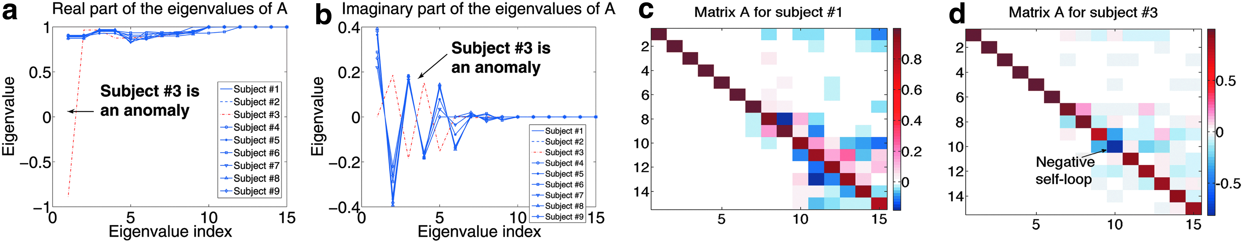
In Figure 5a and b we show the real and imaginary parts of the eigenvalues of A. We can see that for eight human subjects, the eigenvalues are almost identical. This finding agrees with neuroscientific results on different experimental settings,18 further demonstrating GeBM's ability to provide useful insights on multisubject experiments. For subject no. 3 there is a deviation on the real part of the first eigenvalue, as well as a slightly deviating pattern on the imaginary parts of its eigenvalues. Figures 5c and d compare matrix A for subjects 1 and 3. There is a unique fact pertaining to subject no. 3's connectivity matrix: there is a negative value on the diagonal [blue square at the (8, 8) entry], in other words, a negative self-loop in the connectivity graph, which causes the differences in the behavior of subject no. 3's system.
Multisubject analysis: Panels (a) and (b) show the real and imaginary parts of the eigenvalues of matrix A for each subject. For all subjects but one (subject no. 3) the eigenvalues are almost identical, implying that the GeBM that captures their brain activity behaves more or less in the same way. Subject no. 3 on the other hand is an outlier; indeed, during the experiment, the subject complained that he was able to hear a demonstration happening outside of the laboratory, rendering the experimental task assigned to the subject more difficult than it was supposed to be. Panels (c) and (d) show matrices A for subjects no. 1 and no. 3. Subject no. 3's matrix seems sparser and most importantly, we can see that there is a negative entry on the diagonal, a fact unique to subject no. 3.
According to neuroscientific studies (e.g., He et al.19), the first “culprit” for causing such a discrepancy in the estimated model would be the handedness of subject no. 3. However, as we highlighted in the beginning of the section, all nine human subjects were right-handed, and thus, difference in handedness cannot be a plausible explanation for this anomaly.
We subsequently turned our attention to the conditions under which the experiment was conducted, and according to the person responsible for the data collection of subject no. 3: “There was a big demonstration outside the UPMC building during the scan, and I remember the subject complaining during one of the breaks that he could hear the crowd shouting through the walls.”
This is a plausible explanation for the deviation of GeBM for subject no. 3.
5.3. D3: Brain activity simulation
An additional way to gain confidence in our model is to assess its ability to simulate/predict brain activity, given the inferred functional connectivity. In order to do so, we trained GeBM using data from all but one of the words, and then we simulated brain activity time-series for the left-out word. In lieu of competing methods, we compare our proposed method GeBM against our initial approach (whose unsuitability we have argued for in section 3, but we use here in order to further solidify our case). As an initial state for GeBM, we use C†y(0), and for Model0, we simply use y(0). The final time-series we show, both for the real data and the estimated ones, are normalized to unit norm and plotted in absolute values. For exposition purposes, we sorted the voxels according to the ℓ2 norm of their time series vector, and we are displaying the high-ranking ones (however, the same pattern holds for all voxels).
In Figure 6 we illustrate the simulated brain activity of GeBM (solid red), compared against the ones of Model0 (using LS, dash-dot magenta, and CCA, dashed black), as well as the original brain activity time series (dashed blue) for the four highest ranking voxels. Clearly, the activity generated using GeBM is far more realistic than the results of Model0.
Effective brain activity simulation: Comparison of the real brain activity and the simulated ones using GeBM and Model0 for the first four high ranking voxels (in the ℓ2 norm sense).
5.4. D4: Explanation of psychological phenomena
As we briefly mentioned in the introduction, we would like our proposed method to be able to capture some of the psychological phenomena that the human brain exhibits. We by no means claim that GeBM is able to capture convoluted still little-understood physiological phenomena, however, in this section we demonstrate GeBM's ability to simulate two very basic phenomena, habituation and priming. Unlike the previous discoveries, the following experiments are on synthetic data, and their purpose is to showcase GeBM's additional strengths.
Habituation
In our simplified version of habituation, we observe the demand behavior: Given a repeated stimulus, the neurons initially get activated, but their activation levels decline (t=60 in Fig. 7) if the stimulus persists for a long time (t=80 in Fig. 7). In Figure. 7, we show that GeBM is able to capture such behavior. In particular, we show the desired input and output for a few (observed) voxels, and we show, given the functional connectivity obtained according to GeBM, the simulated output, which exhibits the same desired behavior. In order to simplify the training data generation, we produce an instantaneous “switch-off” of the activity in the desired output, which is a crude approximation of a gradual attenuation, which is expected. Remarkably, though, GeBM (using Algorithm 1) is able to produce a very realistic, gradually attenuating activity curve.
GeBM captures Habituation: Given repeated exposure to a stimulus, the brain activity starts to fade.
Priming
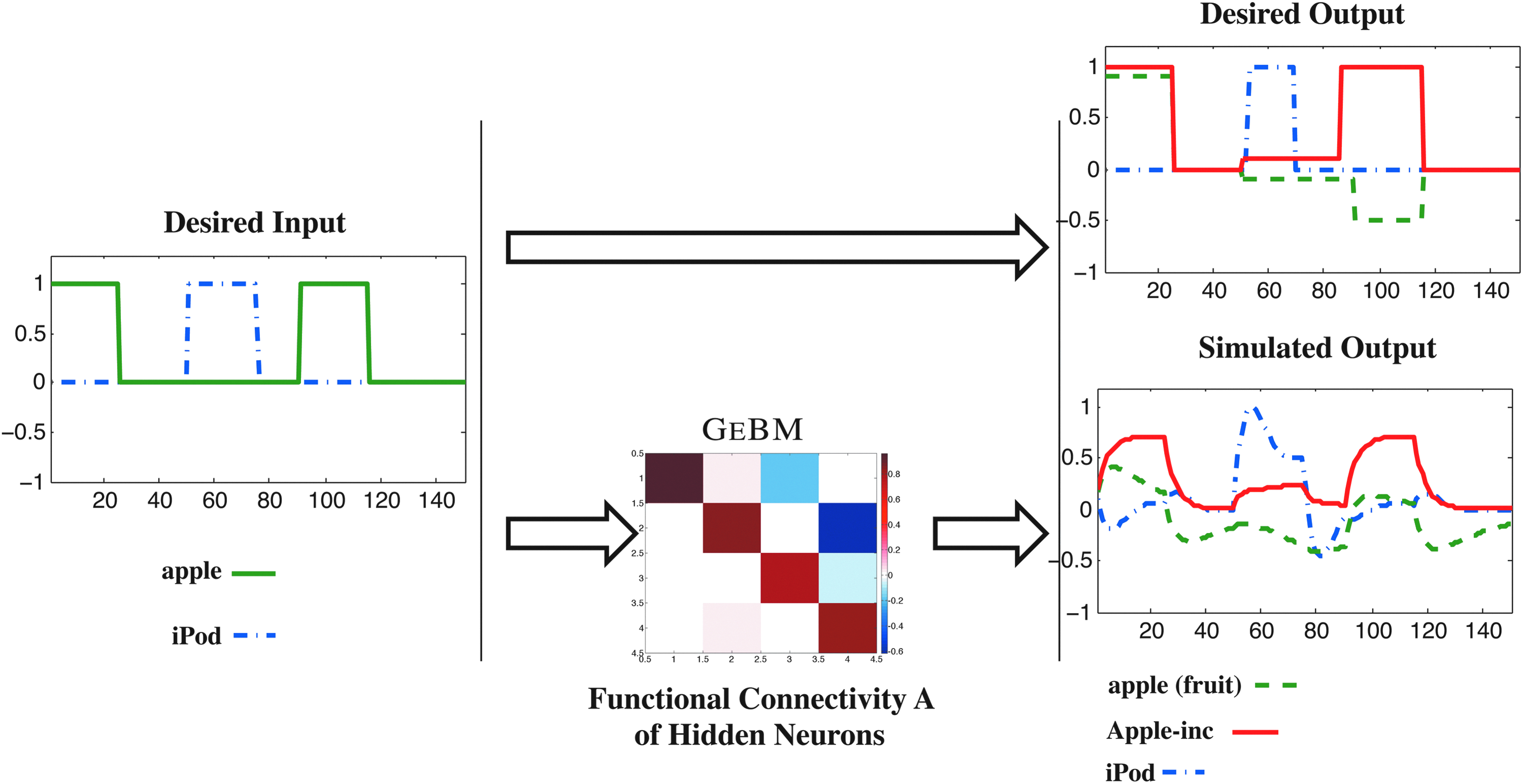
In our simplified model on priming, first we give the stimulus apple, which sets off neurons that are associated with the fruit “apple,” as well as neurons that are associated with Apple, Inc. Subsequently, we are showing a stimulus such as an iPod; this predisposes the regions of the brain that are associated with Apple, Inc., to display some small level of activation, whereas suppressing the regions of the brain that are associated with apple (the fruit). Later on, the stimulus apple is repeated, which, given the aforementioned predisposition, activates the voxels associated with Apple (company) and suppresses the ones associated with the homonymous fruit.
Figure 8 displays a pictorial description of the above example of priming; given desired input/output training pairs, we derive a model that obeys GeBM using our proposed Algorithm 1, such that we match the priming behavior.
GeBm captures Priming: When first shown the stimulus apple, both neurons associated with the fruit apple and Apple, Inc. are activated. When showing the stimulus iPod and then apple, iPod predisposes the neurons associated with Apple, Inc., to get activated more quickly, while suppressing the ones associated with the fruit.
6. Related Work
“ESTIMATING THE BRAIN'S FUNCTIONAL CONNECTIVITY IS AN ACTIVE FIELD OF STUDY OF COMPUTATIONAL NEUROSCIENCE.”
Brain functional connectivity: Estimating the brain's functional connectivity is an active field of study of computational neuroscience. Examples of works can be found in Refs.7,20,21. There have been a few works in the data mining community as well: In Sun et al. (2009)9, the authors derive the brain region connections for Alzheimer's patients, and recently22 that leverages tensor decomposition in order to discover the underlying network of the human brain. Most related to the present work is the work of Valdes-Sosa et al.23, wherein the authors propose an autoregressive model (similar to Model0) and solve it using regularized regression. However, to the best of our knowledge, this work is the first to apply system identification concepts to this problem.
Psychological phenomena: A concise overview of literature pertaining to habitutation can be found in Thompson and Spencer (1966).24 A more recent study on habitutation can be found in Rankin et al. (2009).25 The definition of priming, as we describe it in the lines above, concurs with the definition found in Friederici (1999). Additionally, in Pickering and Branigan (1998), the authors conduct a study on the effects of priming when the human subjects were asked to write sentences. The above concepts of priming and habituation have also been studied in the context of spreading activation,28,29 which is a model of the cognitive process of memory.
Control theory & system identification: System identification is a field of control theory. In the appendix of our KDD paper5 we provide more theoretical details on subspace system identification, however, Ljung (1999) and Verhaegen and Verdult (2007)14,30 are the most prominent sources for system identification algorithms.
Network discovery from time series: Our work touches upon discovering underlying network structures from time series data; an exemplary work related to the present article is Verscheure (2006),1 in which the authors derive a who-calls-whom network from VoIP packet transmission time series.
7. Conclusions
In this work, we make the following contributions:
• Analytical model & algorithm: We propose GeBM, a novel model of the human brain functional connectivity. We also introduce Sparse-SysId, a novel sparse system identification algorithm that estimates GeBM.
• Effectiveness: GeBM simulates psychological phenomena (such as habituation and priming), as well as provides valuable neuroscientific insights.
• Validation: We validate our approach on real data, where our model produces brain activity patterns, remarkably similar to the true ones.
• Multisubject analysis: We analyze measurements from nine human subjects, identifying a consistent connectivity among eight of them; we successfully identify an outlier, whose experimental procedure was compromised.
• Cross-disciplinary connections: We highlight connections between disparate areas: (1) neuroscience, (2) control theory & system identification, and (3) psychology, and we provide insights on the relation of GeBM to recurrent neural networks.
The problem of identifying the functional connectivity of the human brain is very important in the field of neuroscience, as it contributes to our knowledge about how the human brain operates and processes information. However, solving this problem can have applications that go far beyond neuroscience:
• Improving artificial intelligence & machine learning: Having a better understanding of how the human brain processes information is of paramount importance in the design of intelligent algorithms; in particular, such understanding can be greatly beneficial, especially to fields that are inspired by the way that the human brain operates, with a prime example of deep learning,31 which is gaining increasing attention.
• Detecting & ameliorating learning disorders: On a different spin, understanding the functional connectivity of the brain can be used in order to detect learning disorders in children, at a very early stage, in a noninvasive way. If we have a model for the functional connectivity, as well as an understanding of how different learning disorders may perturb that model, we might be able to, first, detect the disorder, and subsequently, by targeting the child's education and closely monitoring changes in the connectivity, we may be able to ameliorate the effects of certain disorders.
Footnotes
Acknowledgments
Research was supported by grants NSF IIS-1247489, NSF IIS-1247632, NSF CDI 0835797, NIH/NICHD 12165321, DARPA FA87501320005, and IARPA FA865013C7360, and by Google. This work was also supported in part by a fellowship to Alona Fyshe from the Multimodal Neuroimaging Training Program funded by NIH grants T90DA022761 and R90DA023420. Any opinions, findings, and conclusions or recommendations expressed in this material are those of the authors and do not necessarily reflect the views of the funding parties. We would also like to thank Erika Laing and the UPMC Brain Mapping Center for their help with the data and visualization of our results. Finally, we would like to thank Gustavo Sudre for collecting and sharing the data, and Dr. Brian Murphy for valuable conversations.
Author Disclosure Statement
No competing financial interests exist.
References
1.
VerscheureD, VlachosM, AnagnostopoulosA, et al.Finding “who is talking to whom” in voip networks via progressive stream clustering. In: Proceedings of the IEEE ICDM, 667–677. IEEE 2006.
2.
SadilekA, KautzH, and BighamJP. Finding your friends and following them to where you are. In: Proceedings of the Fifth ACM International Conference on Web Search and Data mining, 723–732. ACM. 2012.
3.
WilliamsRN and HerrupK. The control of neuron number. Annual Review of Neuroscience, 1988, 11:423–453.
4.
AzevedoFAC, CarvalhoLRB, GrinbergLT, et al.Equal numbers of neuronal and nonneuronal cells make the human brain an isometrically scaled-up primate brain. Journal of Comparative Neurology, 2009, 513:532–541.
5.
PapalexakisEE, FysheA, SidiropoulosND, et al.Good-enough brain model: challenges, algorithms and discoveries in multi-subject experiments. In: Proceedings of the 20th ACM SIGKDD International Conference on Knowledge Discovery and Data Mining, 95–104. ACM. 2014.
6.
SudreG, PomerleauD, PalatucciM, et al.Tracking neural coding of perceptual and semantic features of concrete nouns. NeuroImage, 2012, 62:451–463.
7.
FysheA, FoxEB, DunsonDB, and MitchellTM. Hierarchical latent dictionaries for models of brain activation. AISTATS JMLR, 2012, 22:409–421.
8.
SchizasID, GiannakisGB, and LuoZ-Q. Distributed estimation using reduced-dimensionality sensor observations. IEEE TSP, 2007, 55:4284–4299.
9.
SunL, PatelRJ, Mining brain region connectivity for alzheimer's disease study via sparse inverse covariance estimation. In: Proceedings of the ACM SIGKDD, 1335–1344. ACM 2009.
10.
JaegerH. Tutorial on training recurrent neural networks, covering BPPT, RTRL, EKF and the “echo state network” approach. GMD-Forschungszentrum Informationstechnik, 2002.
11.
JaegerH. Echo state network. Scholarpedia. 2007, 2:2330.
12.
JaegerH. The Jecho state approach to analysing and training recurrent neural networks-with an erratum note. German National Research Center for Information Technology GMD Technical Report, 2001, 148:34.
13.
JaegerH. Adaptive nonlinear system identification with echo state networks. Advances in Neural Information Processing Systems, 2002, 593–600.
14.
LjungL. System identification. Wiley Online Library. 1999.
15.
VerhaegenM. Identification of the deterministic part of mimo state space models given in innovations form from input-output data. Automatica, 1994, 30:61–74.
16.
HickokG and PoeppelD. aDorsal and ventral streams: a framework for understanding aspects of the functional anatomy of language. Cognition, 2004, 92:67–99.
17.
BinderJR and DesaiRH. The neurobiology of semantic memory. Trends in Cognitive Sciences, 2011, 15:527–536.
18.
TomasiD and VolkowND. Resting functional connectivity of language networks: characterization and reproducibility. Molecular Psychiatry, 2012, 17:841–854.
19.
HeY, ZangY, JiangT, et al.Handedness-related functional connectivity using low-frequency blood oxygenation level-dependent fluctuations. Neuroreport, 2006, 17:5–8.
20.
SakkalisV. Review of advanced techniques for the estimation of brain connectivity measured with eeg/meg. Computers in Biology and Medicine, 2011, 41:1110–1117.
21.
GreiciusMD, KrasnowB, ReissAL, and MenonV. Functional connectivity in the resting brain: a network analysis of the default mode hypothesis. PNAS, 2003, 100:253–258.
22.
DavidsonI, GilpinS, CarmichaelO, and WalkerP. Network discovery via constrained tensor analysis of fmri data. In: Proceedings of the ACM SIGKDD, ACM 2013, 194–202.
23.
Valdés-SosaPA, Sánchez-BornotJM, Lage-CastellanosAet al.Estimating brain functional connectivity with sparse multivariate autoregression. Philosophical Transactions of the Royal Society B: Biological Sciences, 2005, 360:969–981.
24.
ThompsonRF and SpencerWA. Habituation: a model phenomenon for the study of neuronal substrates of behavior. Psychological Review, 1966, 73:16.
25.
RankinCH, AbramsT, BarryRJ, Habituation revisited: an updated and revised description of the behavioral characteristics of habituation. Neurobiology of Learning and Memory, 2009, 92:135–138.
26.
FriedericiAD, SteinhauerK, and FrischS. Lexical integration: Sequential effects of syntactic and semantic information. Memory & Cognition, 1999, 27:438–453.
27.
PickeringMJ and BraniganHP. The representation of verbs: Evidence from syntactic priming in language production. Journal of Memory and Language, 1998, 39:633–651.
28.
AndersonJR. A spreading activation theory of memory. Journal of Verbal Learning and Verbal behavior, 1983, 22:261–295.
29.
CollinsAM. LoftusEF. A spreading-activation theory of semantic processing. Psychological Review, 1975, 82:407–428.
30.
VerhaegenM and VerdultV. Filtering and system identification: a least squares approach. New York: Cambridge University Press. 2007.
31.
SchmidhuberJ. Deep learning in neural networks: An overview. CoRR, 2014, abs/1404.7828.