Recidivism prediction instruments (RPIs) provide decision-makers with an assessment of the likelihood that a criminal defendant will reoffend at a future point in time. Although such instruments are gaining increasing popularity across the country, their use is attracting tremendous controversy. Much of the controversy concerns potential discriminatory bias in the risk assessments that are produced. This article discusses several fairness criteria that have recently been applied to assess the fairness of RPIs. We demonstrate that the criteria cannot all be simultaneously satisfied when recidivism prevalence differs across groups. We then show how disparate impact can arise when an RPI fails to satisfy the criterion of error rate balance.
Introduction
Risk assessment instruments are gaining increasing popularity within the criminal justice system, with versions of such instruments being used or considered for use in pretrial decision-making, parole decisions, and in some states even sentencing.1–3 In each of these cases, a high-risk classification—particularly a high-risk misclassification—may have a direct adverse impact on a criminal defendant's outcome. If the use of recidivism prediction instruments (RPIs) is to become commonplace, it is especially important to ensure that the instruments are free from discriminatory biases that could result in unethical practices and inequitable outcomes for different groups.
In a recent widely popularized investigation conducted by a team at ProPublica, Angwin et al.4 studied an RPI called COMPAS,* concluding that it is biased against black defendants. The authors found that the likelihood of a nonrecidivating black defendant being assessed as high risk is nearly twice that of white defendants. Similarly, the likelihood of a recidivating black defendant being assessed as low risk is nearly half that of white defendants. In technical terms, these findings indicate that the COMPAS instrument has considerably higher false positive rates (FPRs) and lower false negative rates (FNRs) for black defendants than for white defendants.
ProPublica's analysis has met with much criticism both from the academic community and from the Northpointe corporation. Much of the criticism has focused on the particular choice of fairness criteria selected for the investigation. Flores et al.6 argue that the correct approach for assessing RPI bias is instead to check for calibration, a fairness criterion that they show COMPAS satisfies. Northpointe in its response7 argues for a still different approach that checks for a fairness criterion termed predictive parity, which it demonstrates COMPAS also satisfies. We provide precise definitions and a more in-depth discussion of these and other fairness criteria in the Background section.
In this article we show that the differences in FPRs and FNRs cited as evidence of racial bias by Angwin et al.4 are a direct consequence of applying an RPI that satisfies predictive parity to a population in which recidivism prevalence† differs across groups. Our main contribution is twofold. (1) First, we make precise the connection between the predictive parity criterion and error rates in classification. (2) Next, we demonstrate how using an RPI that has different FPRs and FNRs between groups can lead to disparate impact when individuals assessed as high risk receive stricter penalties. Throughout our discussion we use the term disparate impact to refer to settings wherein a penalty policy has unintended disproportionate adverse impact on a particular group.
It is important to bear in mind that fairness itself—along with the notion of disparate impact—is a social and ethical concept, not a statistical concept. A risk prediction instrument that is fair with respect to particular fairness criteria may nevertheless result in disparate impact depending on how and where it is used. In this article, we consider hypothetical use cases in which we are able to directly connect particular fairness properties of an RPI to a measure of disparate impact. We present both theoretical and empirical results to illustrate how disparate impact can arise.
Outline of the article
We begin in the Assessing Fairness section by providing some background on several of the different fairness criteria that have appeared in recent literature. We then proceed to demonstrate that an instrument that satisfies predictive parity cannot have equal FPRs and FNRs across groups when the recidivism prevalence differs across those groups. In the Assessing Impact section, we analyze a simple risk assessment-based sentencing policy and show how differences in FPRs and FNRs can result in disparate impact under this policy. In the Empirical Results section, we back up our theoretical analysis by presenting some empirical results based on the data made available by the ProPublica investigators. We conclude in the Discussion section with some remarks concerning the issues that data bias presents for the arguments put forth in this article.
Data description and setup
The empirical results in this article are based on the Broward County data made publicly available by ProPublica.8 This data set contains COMPAS recidivism risk decile scores, 2-year recidivism outcomes, and a number of demographic and crime-related variables on individuals who were scored in 2013 and 2014. We restrict our attention to the subset of defendants whose race is recorded as African American (b) or Caucasian (w).‡ After applying the same data preprocessing and filtering as reported in the ProPublica analysis, we are left with a data set on \documentclass{aastex}\usepackage{amsbsy}\usepackage{amsfonts}\usepackage{amssymb}\usepackage{bm}\usepackage{mathrsfs}\usepackage{pifont}\usepackage{stmaryrd}\usepackage{textcomp}\usepackage{portland, xspace}\usepackage{amsmath, amsxtra}\usepackage{upgreek}\pagestyle{empty}\DeclareMathSizes{10}{9}{7}{6}\begin{document}
$$n = 6150$$
\end{document} individuals, of whom \documentclass{aastex}\usepackage{amsbsy}\usepackage{amsfonts}\usepackage{amssymb}\usepackage{bm}\usepackage{mathrsfs}\usepackage{pifont}\usepackage{stmaryrd}\usepackage{textcomp}\usepackage{portland, xspace}\usepackage{amsmath, amsxtra}\usepackage{upgreek}\pagestyle{empty}\DeclareMathSizes{10}{9}{7}{6}\begin{document}
$${n_b} = 3696$$
\end{document} are African American and \documentclass{aastex}\usepackage{amsbsy}\usepackage{amsfonts}\usepackage{amssymb}\usepackage{bm}\usepackage{mathrsfs}\usepackage{pifont}\usepackage{stmaryrd}\usepackage{textcomp}\usepackage{portland, xspace}\usepackage{amsmath, amsxtra}\usepackage{upgreek}\pagestyle{empty}\DeclareMathSizes{10}{9}{7}{6}\begin{document}
$${n_c} = 2454$$
\end{document} are Caucasian.
Assessing Fairness
Background
We begin with some notation. Let \documentclass{aastex}\usepackage{amsbsy}\usepackage{amsfonts}\usepackage{amssymb}\usepackage{bm}\usepackage{mathrsfs}\usepackage{pifont}\usepackage{stmaryrd}\usepackage{textcomp}\usepackage{portland, xspace}\usepackage{amsmath, amsxtra}\usepackage{upgreek}\pagestyle{empty}\DeclareMathSizes{10}{9}{7}{6}\begin{document}
$$S = S ( x )$$
\end{document} denote the risk score based on covariates \documentclass{aastex}\usepackage{amsbsy}\usepackage{amsfonts}\usepackage{amssymb}\usepackage{bm}\usepackage{mathrsfs}\usepackage{pifont}\usepackage{stmaryrd}\usepackage{textcomp}\usepackage{portland, xspace}\usepackage{amsmath, amsxtra}\usepackage{upgreek}\pagestyle{empty}\DeclareMathSizes{10}{9}{7}{6}\begin{document}
$$X = x \in { \mathbb{R}^p}$$
\end{document}, with higher values of S corresponding to higher levels of assessed risk. We interchangeably refer to S as a score or an instrument. For simplicity, our discussion of fairness criteria will focus on a setting wherein there exist just two groups. We let \documentclass{aastex}\usepackage{amsbsy}\usepackage{amsfonts}\usepackage{amssymb}\usepackage{bm}\usepackage{mathrsfs}\usepackage{pifont}\usepackage{stmaryrd}\usepackage{textcomp}\usepackage{portland, xspace}\usepackage{amsmath, amsxtra}\usepackage{upgreek}\pagestyle{empty}\DeclareMathSizes{10}{9}{7}{6}\begin{document}
$$R \in \{ b , w \} $$
\end{document} denote the group to which an individual belongs and do not preclude R from being one of the elements of X. We denote the outcome indicator by \documentclass{aastex}\usepackage{amsbsy}\usepackage{amsfonts}\usepackage{amssymb}\usepackage{bm}\usepackage{mathrsfs}\usepackage{pifont}\usepackage{stmaryrd}\usepackage{textcomp}\usepackage{portland, xspace}\usepackage{amsmath, amsxtra}\usepackage{upgreek}\pagestyle{empty}\DeclareMathSizes{10}{9}{7}{6}\begin{document}
$$Y \in \{ 0 , 1 \} $$
\end{document}, with \documentclass{aastex}\usepackage{amsbsy}\usepackage{amsfonts}\usepackage{amssymb}\usepackage{bm}\usepackage{mathrsfs}\usepackage{pifont}\usepackage{stmaryrd}\usepackage{textcomp}\usepackage{portland, xspace}\usepackage{amsmath, amsxtra}\usepackage{upgreek}\pagestyle{empty}\DeclareMathSizes{10}{9}{7}{6}\begin{document}
$$Y = 1$$
\end{document} indicating that the given individual goes on to recidivate. Lastly, we introduce the quantity \documentclass{aastex}\usepackage{amsbsy}\usepackage{amsfonts}\usepackage{amssymb}\usepackage{bm}\usepackage{mathrsfs}\usepackage{pifont}\usepackage{stmaryrd}\usepackage{textcomp}\usepackage{portland, xspace}\usepackage{amsmath, amsxtra}\usepackage{upgreek}\pagestyle{empty}\DeclareMathSizes{10}{9}{7}{6}\begin{document}
$${s_{{ \rm{HR}}}}$$
\end{document}, which denotes the high-risk score threshold. Defendants whose score S exceeds \documentclass{aastex}\usepackage{amsbsy}\usepackage{amsfonts}\usepackage{amssymb}\usepackage{bm}\usepackage{mathrsfs}\usepackage{pifont}\usepackage{stmaryrd}\usepackage{textcomp}\usepackage{portland, xspace}\usepackage{amsmath, amsxtra}\usepackage{upgreek}\pagestyle{empty}\DeclareMathSizes{10}{9}{7}{6}\begin{document}
$${s_{{ \rm{HR}}}}$$
\end{document} are referred to as high risk, whereas the remaining defendants are referred to as low risk.
With this notation in hand, we now proceed to define and discuss several fairness criteria that commonly appear in the literature, beginning with those mentioned in the Introduction section. We indicate cases wherein a given criterion is known to us to also commonly appear under some other name. All of the criteria presented hereunder can also be assessed conditionally by further conditioning on some covariates in X. We discuss this point in greater detail in the Conditioning on Other Covariates section.
Definition 1 (Calibration). A score\documentclass{aastex}\usepackage{amsbsy}\usepackage{amsfonts}\usepackage{amssymb}\usepackage{bm}\usepackage{mathrsfs}\usepackage{pifont}\usepackage{stmaryrd}\usepackage{textcomp}\usepackage{portland, xspace}\usepackage{amsmath, amsxtra}\usepackage{upgreek}\pagestyle{empty}\DeclareMathSizes{10}{9}{7}{6}\begin{document}
$$S = S ( x )$$
\end{document}is said to be well calibrated if it reflects the same likelihood of recidivism irrespective of the individuals' group membership. That is, if for all values of s,\documentclass{aastex}\usepackage{amsbsy}\usepackage{amsfonts}\usepackage{amssymb}\usepackage{bm}\usepackage{mathrsfs}\usepackage{pifont}\usepackage{stmaryrd}\usepackage{textcomp}\usepackage{portland, xspace}\usepackage{amsmath, amsxtra}\usepackage{upgreek}\pagestyle{empty}\DeclareMathSizes{10}{9}{7}{6}\begin{document}
\begin{align*}
\mathbb{P} ( Y = 1 \vert S = s , R = b ) = \mathbb{P} ( Y = 1 \vert S = s , R = w ). \tag{2.1}
\end{align*}
\end{document}
Within the educational and psychological testing and assessment literature, the notion of calibration features among the widely accepted and adopted standards for empirical fairness assessment. In this literature, an instrument that is well calibrated is referred to as being free from predictive bias or differential prediction. This criterion has recently been applied to the PCRA§ instrument, with initial findings suggesting that calibration is satisfied with respect to race10,11 but not with respect to gender.12 In their response to the ProPublica investigation, Flores et al.6 verify that COMPAS is well calibrated using logistic regression modeling.
Definition 2 (Predictive parity). A score\documentclass{aastex}\usepackage{amsbsy}\usepackage{amsfonts}\usepackage{amssymb}\usepackage{bm}\usepackage{mathrsfs}\usepackage{pifont}\usepackage{stmaryrd}\usepackage{textcomp}\usepackage{portland, xspace}\usepackage{amsmath, amsxtra}\usepackage{upgreek}\pagestyle{empty}\DeclareMathSizes{10}{9}{7}{6}\begin{document}
$$S = S ( x )$$
\end{document} satisfies predictive parity at a threshold \documentclass{aastex}\usepackage{amsbsy}\usepackage{amsfonts}\usepackage{amssymb}\usepackage{bm}\usepackage{mathrsfs}\usepackage{pifont}\usepackage{stmaryrd}\usepackage{textcomp}\usepackage{portland, xspace}\usepackage{amsmath, amsxtra}\usepackage{upgreek}\pagestyle{empty}\DeclareMathSizes{10}{9}{7}{6}\begin{document}
$${s_{{ \rm{HR}}}}$$
\end{document} if the likelihood of recidivism among high-risk offenders is the same regardless of group membership. That is, if
\documentclass{aastex}\usepackage{amsbsy}\usepackage{amsfonts}\usepackage{amssymb}\usepackage{bm}\usepackage{mathrsfs}\usepackage{pifont}\usepackage{stmaryrd}\usepackage{textcomp}\usepackage{portland, xspace}\usepackage{amsmath, amsxtra}\usepackage{upgreek}\pagestyle{empty}\DeclareMathSizes{10}{9}{7}{6}\begin{document}
\begin{align*}
\mathbb{P} ( Y = 1 \vert S > {s_{{ \rm{HR}}}} , R = b ) = \mathbb{P} ( Y = 1 \vert S > {s_{{ \rm{HR}}}} , R = w ). \tag{2.2}
\end{align*}
\end{document}
Predictive parity at a given threshold \documentclass{aastex}\usepackage{amsbsy}\usepackage{amsfonts}\usepackage{amssymb}\usepackage{bm}\usepackage{mathrsfs}\usepackage{pifont}\usepackage{stmaryrd}\usepackage{textcomp}\usepackage{portland, xspace}\usepackage{amsmath, amsxtra}\usepackage{upgreek}\pagestyle{empty}\DeclareMathSizes{10}{9}{7}{6}\begin{document}
$${s_{{ \rm{HR}}}}$$
\end{document} amounts to requiring that the positive predictive value (PPV) of the classifier \documentclass{aastex}\usepackage{amsbsy}\usepackage{amsfonts}\usepackage{amssymb}\usepackage{bm}\usepackage{mathrsfs}\usepackage{pifont}\usepackage{stmaryrd}\usepackage{textcomp}\usepackage{portland, xspace}\usepackage{amsmath, amsxtra}\usepackage{upgreek}\pagestyle{empty}\DeclareMathSizes{10}{9}{7}{6}\begin{document}
$$\hat Y{ = {\mathbb 1}_{S > {s_{{ \rm{HR}}}}}}$$
\end{document} be the same across groups. Although predictive parity and calibration look like very similar criteria, well-calibrated scores can fail to satisfy predictive parity at a given threshold. This is because the relationship between Equations (2.2) and (2.1) depends on the conditional distribution of \documentclass{aastex}\usepackage{amsbsy}\usepackage{amsfonts}\usepackage{amssymb}\usepackage{bm}\usepackage{mathrsfs}\usepackage{pifont}\usepackage{stmaryrd}\usepackage{textcomp}\usepackage{portland, xspace}\usepackage{amsmath, amsxtra}\usepackage{upgreek}\pagestyle{empty}\DeclareMathSizes{10}{9}{7}{6}\begin{document}
$$S \vert R = r$$
\end{document}, which can differ across groups in ways that result in PPV imbalance. In the simple case wherein S itself is binary, a score that is well calibrated will also satisfy predictive parity. Northpointe's refutation7 of the ProPublica analysis shows that COMPAS satisfies predictive parity for threshold choices of interest.
Definition 3 (Error rate balance). A score \documentclass{aastex}\usepackage{amsbsy}\usepackage{amsfonts}\usepackage{amssymb}\usepackage{bm}\usepackage{mathrsfs}\usepackage{pifont}\usepackage{stmaryrd}\usepackage{textcomp}\usepackage{portland, xspace}\usepackage{amsmath, amsxtra}\usepackage{upgreek}\pagestyle{empty}\DeclareMathSizes{10}{9}{7}{6}\begin{document}
$$S = S ( x )$$
\end{document} satisfies error rate balance at a threshold \documentclass{aastex}\usepackage{amsbsy}\usepackage{amsfonts}\usepackage{amssymb}\usepackage{bm}\usepackage{mathrsfs}\usepackage{pifont}\usepackage{stmaryrd}\usepackage{textcomp}\usepackage{portland, xspace}\usepackage{amsmath, amsxtra}\usepackage{upgreek}\pagestyle{empty}\DeclareMathSizes{10}{9}{7}{6}\begin{document}
$${s_{{ \rm{HR}}}}$$
\end{document} if the false positive and false negative error rates are equal across groups. That is, if
\documentclass{aastex}\usepackage{amsbsy}\usepackage{amsfonts}\usepackage{amssymb}\usepackage{bm}\usepackage{mathrsfs}\usepackage{pifont}\usepackage{stmaryrd}\usepackage{textcomp}\usepackage{portland, xspace}\usepackage{amsmath, amsxtra}\usepackage{upgreek}\pagestyle{empty}\DeclareMathSizes{10}{9}{7}{6}\begin{document}
\begin{align*}
\mathbb{P} ( S > {s_{{ \rm{HR}}}} \vert Y = 0 , R = b ) = \mathbb{P} ( S > {s_{{ \rm{HR}}}} \vert Y = 0 , R = w ) \;{ \rm{and}} \tag{2.3}
\end{align*}
\end{document}\documentclass{aastex}\usepackage{amsbsy}\usepackage{amsfonts}\usepackage{amssymb}\usepackage{bm}\usepackage{mathrsfs}\usepackage{pifont}\usepackage{stmaryrd}\usepackage{textcomp}\usepackage{portland, xspace}\usepackage{amsmath, amsxtra}\usepackage{upgreek}\pagestyle{empty}\DeclareMathSizes{10}{9}{7}{6}\begin{document}
\begin{align*}
\mathbb{P} ( S \le {s_{{ \rm{HR}}}} \vert Y = 1 , R = b ) = \mathbb{P} ( S \le {s_{{ \rm{HR}}}} \vert Y = 1 , R = w ) , \tag{2.4}
\end{align*}
\end{document}
where the expressions in the first line are the group-specific FPRs and those in the second line are the group-specific FNRs.
ProPublica's analysis considered a threshold of \documentclass{aastex}\usepackage{amsbsy}\usepackage{amsfonts}\usepackage{amssymb}\usepackage{bm}\usepackage{mathrsfs}\usepackage{pifont}\usepackage{stmaryrd}\usepackage{textcomp}\usepackage{portland, xspace}\usepackage{amsmath, amsxtra}\usepackage{upgreek}\pagestyle{empty}\DeclareMathSizes{10}{9}{7}{6}\begin{document}
$${s_{{ \rm{HR}}}} = 4$$
\end{document}, which they showed leads to considerable imbalance in both FPRs and FNRs. Although this choice of cutoff met with some criticism, we see later in this section that error rate imbalance persists—indeed, must persist—for any choice of cutoff at which the score satisfies the predictive parity criterion. Error rate balance is also closely connected to the notions of equalized odds and equal opportunity as introduced in the recent work of Hardt et al.13
Definition 4 (Statistical parity). A score \documentclass{aastex}\usepackage{amsbsy}\usepackage{amsfonts}\usepackage{amssymb}\usepackage{bm}\usepackage{mathrsfs}\usepackage{pifont}\usepackage{stmaryrd}\usepackage{textcomp}\usepackage{portland, xspace}\usepackage{amsmath, amsxtra}\usepackage{upgreek}\pagestyle{empty}\DeclareMathSizes{10}{9}{7}{6}\begin{document}
$$S = S ( x )$$
\end{document} satisfies statistical parity at a threshold \documentclass{aastex}\usepackage{amsbsy}\usepackage{amsfonts}\usepackage{amssymb}\usepackage{bm}\usepackage{mathrsfs}\usepackage{pifont}\usepackage{stmaryrd}\usepackage{textcomp}\usepackage{portland, xspace}\usepackage{amsmath, amsxtra}\usepackage{upgreek}\pagestyle{empty}\DeclareMathSizes{10}{9}{7}{6}\begin{document}
$${s_{{ \rm{HR}}}}$$
\end{document} if the proportion of individuals classified as high risk is the same for each group. That is, if
\documentclass{aastex}\usepackage{amsbsy}\usepackage{amsfonts}\usepackage{amssymb}\usepackage{bm}\usepackage{mathrsfs}\usepackage{pifont}\usepackage{stmaryrd}\usepackage{textcomp}\usepackage{portland, xspace}\usepackage{amsmath, amsxtra}\usepackage{upgreek}\pagestyle{empty}\DeclareMathSizes{10}{9}{7}{6}\begin{document}
\begin{align*}
\mathbb{P} ( S > {s_{{ \rm{HR}}}} \vert R = b ) = \mathbb{P} ( S > {s_{{ \rm{HR}}}} \vert R = w ). \tag{2.5}
\end{align*}
\end{document}
Statistical parity also goes by the name of equal acceptance rates14 or group fairness,15 although it should be noted that these terms are in many cases not used synonymously. Although our discussion focuses primarily on first three fairness criteria, statistical parity is widely used within the machine learning community and may be the criterion with which many readers are most familiar.16,17 Statistical parity is well suited to contexts such as employment or admissions, wherein it may be desirable or required by law or regulation to employ or admit individuals in equal proportion across racial, gender, or geographical groups. It is, however, a difficult criterion to motivate in the recidivism prediction setting, and thus will not be further considered in this work.
Further related work
Although the study of discrimination in decision-making and predictive modeling is rapidly evolving, it also has a long and rich multidisciplinary history. Romei and Ruggieri18 provide an excellent overview of some of the work in this broad subject area. The recent work of Barocas and Selbst19 offers a broad examination of algorithmic fairness framed within the context of antidiscrimination laws governing employment practices. Hannah-Moffat,20 Skeem,21 and Monahan and Skeem22 examine legal and ethical issues relating specifically to the use of risk assessment instruments in sentencing, citing the potential for race and gender discrimination as a major concern.
In work concurrent with our own, several other researchers have also investigated the compatibility of different notions of fairness. Kleinberg et al.23 show that calibration cannot be satisfied simultaneously with the fairness criteria of balance for the negative class and balance for the positive class. Translated into the present context, the latter criteria require that the average score assigned to nonrecidivists (the negative class) should be the same for both groups, and that the same should hold among recidivists (the positive class). The work of Corbett-Davies et al.24 closely parallels the results that we present in the Predictive parity, FPRs, and FNRs section, reaching the same conclusion regarding the incompatibility of predictive parity and error rate balance in the setting of unequal prevalence.
Predictive parity, FPRs, and FNRs
In this section we present our first main result, which establishes that predictive parity is incompatible with error rate balance when prevalence differs across groups. To better motivate the discussion, we begin by presenting an empirical fairness assessment of the COMPAS RPI. Figure 1 shows plots of the observed recidivism rates and error rates corresponding to the fairness notions of calibration, predictive parity, and error rate balance. We see that the COMPAS RPI is (approximately) well calibrated, and also satisfies predictive parity provided that the high-risk cutoff \documentclass{aastex}\usepackage{amsbsy}\usepackage{amsfonts}\usepackage{amssymb}\usepackage{bm}\usepackage{mathrsfs}\usepackage{pifont}\usepackage{stmaryrd}\usepackage{textcomp}\usepackage{portland, xspace}\usepackage{amsmath, amsxtra}\usepackage{upgreek}\pagestyle{empty}\DeclareMathSizes{10}{9}{7}{6}\begin{document}
$${s_{{ \rm{HR}}}}$$
\end{document} is 4 or greater. However, COMPAS fails on both false positive and false negative error rate balance across the range of high-risk cutoffs.
Empirical assessment of the COMPAS RPI according to three of the fairness criteria presented in the Background section. Error bars represent 95% confidence intervals. These figures confirm that COMPAS is (approximately) well calibrated, satisfies predictive parity for high-risk cutoff values of 4 or higher, but fails to have error rate balance. (a) Bars represent empirical estimates of the expressions in Equation (2.1): \documentclass{aastex}\usepackage{amsbsy}\usepackage{amsfonts}\usepackage{amssymb}\usepackage{bm}\usepackage{mathrsfs}\usepackage{pifont}\usepackage{stmaryrd}\usepackage{textcomp}\usepackage{portland, xspace}\usepackage{amsmath, amsxtra}\usepackage{upgreek}\pagestyle{empty}\DeclareMathSizes{10}{9}{7}{6}\begin{document}
$${\mathbb P} ( Y = 1 \vert S = s , R = r )$$
\end{document} for decile scores \documentclass{aastex}\usepackage{amsbsy}\usepackage{amsfonts}\usepackage{amssymb}\usepackage{bm}\usepackage{mathrsfs}\usepackage{pifont}\usepackage{stmaryrd}\usepackage{textcomp}\usepackage{portland, xspace}\usepackage{amsmath, amsxtra}\usepackage{upgreek}\pagestyle{empty}\DeclareMathSizes{10}{9}{7}{6}\begin{document}
$$s \in \{ 1 , \ldots , 10 \} $$
\end{document}. (b) Bars represent empirical estimates of the expressions in Equation (2.2): \documentclass{aastex}\usepackage{amsbsy}\usepackage{amsfonts}\usepackage{amssymb}\usepackage{bm}\usepackage{mathrsfs}\usepackage{pifont}\usepackage{stmaryrd}\usepackage{textcomp}\usepackage{portland, xspace}\usepackage{amsmath, amsxtra}\usepackage{upgreek}\pagestyle{empty}\DeclareMathSizes{10}{9}{7}{6}\begin{document}
$${\mathbb P} ( Y = 1 \vert S > {s_{HR}} , R = r )$$
\end{document} for values of the high-risk cutoff \documentclass{aastex}\usepackage{amsbsy}\usepackage{amsfonts}\usepackage{amssymb}\usepackage{bm}\usepackage{mathrsfs}\usepackage{pifont}\usepackage{stmaryrd}\usepackage{textcomp}\usepackage{portland, xspace}\usepackage{amsmath, amsxtra}\usepackage{upgreek}\pagestyle{empty}\DeclareMathSizes{10}{9}{7}{6}\begin{document}
$${s_{_{HR}}} \in \{ 1 , \ldots , 9 \} $$
\end{document}. (c) Bars represent observed false positive rates, which are empirical estimates of the expressions in Equation (2.3): \documentclass{aastex}\usepackage{amsbsy}\usepackage{amsfonts}\usepackage{amssymb}\usepackage{bm}\usepackage{mathrsfs}\usepackage{pifont}\usepackage{stmaryrd}\usepackage{textcomp}\usepackage{portland, xspace}\usepackage{amsmath, amsxtra}\usepackage{upgreek}\pagestyle{empty}\DeclareMathSizes{10}{9}{7}{6}\begin{document}
$${\mathbb P} ( S > {s_{HR}} , \vert Y = 0 , R = r )$$
\end{document} for values of the high-risk cutoff \documentclass{aastex}\usepackage{amsbsy}\usepackage{amsfonts}\usepackage{amssymb}\usepackage{bm}\usepackage{mathrsfs}\usepackage{pifont}\usepackage{stmaryrd}\usepackage{textcomp}\usepackage{portland, xspace}\usepackage{amsmath, amsxtra}\usepackage{upgreek}\pagestyle{empty}\DeclareMathSizes{10}{9}{7}{6}\begin{document}
$${s_{_{HR}}} \in \{ 1 , \ldots , 9 \} $$
\end{document}. (d) Bars represent observed false negative rates, which are empirical estimates of the expressions in Equation (2.4): \documentclass{aastex}\usepackage{amsbsy}\usepackage{amsfonts}\usepackage{amssymb}\usepackage{bm}\usepackage{mathrsfs}\usepackage{pifont}\usepackage{stmaryrd}\usepackage{textcomp}\usepackage{portland, xspace}\usepackage{amsmath, amsxtra}\usepackage{upgreek}\pagestyle{empty}\DeclareMathSizes{10}{9}{7}{6}\begin{document}
$${\mathbb P} ( S > {s_{HR}} , \vert Y = 0 , R = r )$$
\end{document} for values of the high-risk cutoff \documentclass{aastex}\usepackage{amsbsy}\usepackage{amsfonts}\usepackage{amssymb}\usepackage{bm}\usepackage{mathrsfs}\usepackage{pifont}\usepackage{stmaryrd}\usepackage{textcomp}\usepackage{portland, xspace}\usepackage{amsmath, amsxtra}\usepackage{upgreek}\pagestyle{empty}\DeclareMathSizes{10}{9}{7}{6}\begin{document}
$${s_{_{HR}}} \in \{ 1 , \ldots , 9 \} $$
\end{document}. RPI, recidivism prediction instrument.
Angwin et al.4 focused on a high-risk cutoff of \documentclass{aastex}\usepackage{amsbsy}\usepackage{amsfonts}\usepackage{amssymb}\usepackage{bm}\usepackage{mathrsfs}\usepackage{pifont}\usepackage{stmaryrd}\usepackage{textcomp}\usepackage{portland, xspace}\usepackage{amsmath, amsxtra}\usepackage{upgreek}\pagestyle{empty}\DeclareMathSizes{10}{9}{7}{6}\begin{document}
$${s_{{ \rm{HR}}}} = 4$$
\end{document} for their analysis, which some critics have argued is too low, suggesting that \documentclass{aastex}\usepackage{amsbsy}\usepackage{amsfonts}\usepackage{amssymb}\usepackage{bm}\usepackage{mathrsfs}\usepackage{pifont}\usepackage{stmaryrd}\usepackage{textcomp}\usepackage{portland, xspace}\usepackage{amsmath, amsxtra}\usepackage{upgreek}\pagestyle{empty}\DeclareMathSizes{10}{9}{7}{6}\begin{document}
$${s_{{ \rm{HR}}}} = 7$$
\end{document} is more suitable. As can be seen from Figure 1c and d, significant error rate imbalance persists at this cutoff as well. Moreover, the error rates achieved at so high a cutoff are at odds with evidence suggesting that the use of RPIs is of interest in settings wherein FPRs have a higher cost than FNRs, with relative cost estimates ranging from 2.6 to upwards of 15.25,26
As we now proceed to show, the error rate imbalance exhibited by COMPAS is not a coincidence, nor can it be remedied in the present context. When the recidivism prevalence—that is, the base rate \documentclass{aastex}\usepackage{amsbsy}\usepackage{amsfonts}\usepackage{amssymb}\usepackage{bm}\usepackage{mathrsfs}\usepackage{pifont}\usepackage{stmaryrd}\usepackage{textcomp}\usepackage{portland, xspace}\usepackage{amsmath, amsxtra}\usepackage{upgreek}\pagestyle{empty}\DeclareMathSizes{10}{9}{7}{6}\begin{document}
$$\mathbb{P} ( Y = 1 \vert R = r )$$
\end{document}—differs across groups, any instrument that satisfies predictive parity at a given threshold \documentclass{aastex}\usepackage{amsbsy}\usepackage{amsfonts}\usepackage{amssymb}\usepackage{bm}\usepackage{mathrsfs}\usepackage{pifont}\usepackage{stmaryrd}\usepackage{textcomp}\usepackage{portland, xspace}\usepackage{amsmath, amsxtra}\usepackage{upgreek}\pagestyle{empty}\DeclareMathSizes{10}{9}{7}{6}\begin{document}
$${s_{{ \rm{HR}}}}$$
\end{document}must have imbalanced false positive or false negative error rates at that threshold. To understand why predictive parity and error rate balance are mutually exclusive in the setting of unequal recidivism prevalence, it is instructive to think of how these quantities are all related.
Given a particular choice of \documentclass{aastex}\usepackage{amsbsy}\usepackage{amsfonts}\usepackage{amssymb}\usepackage{bm}\usepackage{mathrsfs}\usepackage{pifont}\usepackage{stmaryrd}\usepackage{textcomp}\usepackage{portland, xspace}\usepackage{amsmath, amsxtra}\usepackage{upgreek}\pagestyle{empty}\DeclareMathSizes{10}{9}{7}{6}\begin{document}
$${s_{{ \rm{HR}}}}$$
\end{document}, we can summarize an instrument's performance in terms of a confusion matrix, as shown in Table 1.
T/F denote true/false and N/P denote negative/positive
For instance, FP is the number of false positives: individuals who are classified as high risk but who do not reoffend.
All of the fairness metrics presented in the Background section can be thought of as imposing constraints on the values (or the distribution of values) in this table. Another constraint—one that we have no direct control over—is imposed by the recidivism prevalence within groups. It is not difficult to show that the prevalence (p), \documentclass{aastex}\usepackage{amsbsy}\usepackage{amsfonts}\usepackage{amssymb}\usepackage{bm}\usepackage{mathrsfs}\usepackage{pifont}\usepackage{stmaryrd}\usepackage{textcomp}\usepackage{portland, xspace}\usepackage{amsmath, amsxtra}\usepackage{upgreek}\pagestyle{empty}\DeclareMathSizes{10}{9}{7}{6}\begin{document}
$${ \rm{PPV}}$$
\end{document}, and false positive and negative error rates (\documentclass{aastex}\usepackage{amsbsy}\usepackage{amsfonts}\usepackage{amssymb}\usepackage{bm}\usepackage{mathrsfs}\usepackage{pifont}\usepackage{stmaryrd}\usepackage{textcomp}\usepackage{portland, xspace}\usepackage{amsmath, amsxtra}\usepackage{upgreek}\pagestyle{empty}\DeclareMathSizes{10}{9}{7}{6}\begin{document}
$${ \rm{FPR}}$$
\end{document}, \documentclass{aastex}\usepackage{amsbsy}\usepackage{amsfonts}\usepackage{amssymb}\usepackage{bm}\usepackage{mathrsfs}\usepackage{pifont}\usepackage{stmaryrd}\usepackage{textcomp}\usepackage{portland, xspace}\usepackage{amsmath, amsxtra}\usepackage{upgreek}\pagestyle{empty}\DeclareMathSizes{10}{9}{7}{6}\begin{document}
$${ \rm{FNR}}$$
\end{document}) are related through the equation
\documentclass{aastex}\usepackage{amsbsy}\usepackage{amsfonts}\usepackage{amssymb}\usepackage{bm}\usepackage{mathrsfs}\usepackage{pifont}\usepackage{stmaryrd}\usepackage{textcomp}\usepackage{portland, xspace}\usepackage{amsmath, amsxtra}\usepackage{upgreek}\pagestyle{empty}\DeclareMathSizes{10}{9}{7}{6}\begin{document}
\begin{align*}
{ \rm { FPR } } = \frac { p } { { 1 - p } } { \frac { 1 - { \rm { PPV } } } { { \rm { PPV } } } } ( 1 - { \rm { FNR } } ). \tag { 2.6 }
\end{align*}
\end{document}
From this simple expression, we can see that if an instrument satisfies predictive parity—that is, if the PPV is the same across groups—but the prevalence differs between groups, the instrument cannot achieve equal FPRs and FNRs across those groups.
This observation enables us to better understand why we observe such large discrepancies in FPR and FNR between black and white defendants in Figure 5. The recidivism rate among black defendants in the data is 51%, compared with 39% for white defendants. Thus at any threshold \documentclass{aastex}\usepackage{amsbsy}\usepackage{amsfonts}\usepackage{amssymb}\usepackage{bm}\usepackage{mathrsfs}\usepackage{pifont}\usepackage{stmaryrd}\usepackage{textcomp}\usepackage{portland, xspace}\usepackage{amsmath, amsxtra}\usepackage{upgreek}\pagestyle{empty}\DeclareMathSizes{10}{9}{7}{6}\begin{document}
$${s_{{ \rm{HR}}}}$$
\end{document} wherein the COMPAS RPI satisfies predictive parity, Equation (2.6) tells us that some level of imbalance in the error rates must exist. Since not all of the fairness criteria can be satisfied at the same time, it becomes important to understand the potential impact of failing to satisfy particular criteria. This question is explored in the context of a hypothetical risk-based sentencing framework in the next section.
Assessing Impact
In this section, we show how differences in FPRs and FNRs can result in disparate impact under policies wherein a high-risk assessment results in a stricter penalty for the defendant. Such situations may arise when risk assessments are used to inform bail, parole, or sentencing decisions. In Pennsylvania and Virginia, for instance, statutes permit the use of RPIs in sentencing, provided that the sentence ultimately falls within accepted guidelines.1 We use the term “penalty” somewhat loosely in this discussion to refer to outcomes in both the pretrial and postconviction phase of legal proceedings. For instance, even though pretrial outcomes such as the amount at which bail is set are not punitive in a legal sense, we nevertheless refer to bail amount as a “penalty” for the purpose of our discussion.
There are notable cases wherein RPIs are used for the express purpose of informing risk reduction efforts. In such settings, individuals assessed as high risk receive what may be viewed as a benefit rather than a penalty. The PCRA score, for instance, is intended to support precisely this type of decision-making at the federal courts level.11 Our analysis in this section specifically addresses use cases wherein high-risk individuals receive stricter penalties.
To begin, consider a setting in which guidelines indicate that a defendant is to receive a penalty \documentclass{aastex}\usepackage{amsbsy}\usepackage{amsfonts}\usepackage{amssymb}\usepackage{bm}\usepackage{mathrsfs}\usepackage{pifont}\usepackage{stmaryrd}\usepackage{textcomp}\usepackage{portland, xspace}\usepackage{amsmath, amsxtra}\usepackage{upgreek}\pagestyle{empty}\DeclareMathSizes{10}{9}{7}{6}\begin{document}
$${t_{{ \rm{min}}}} \le T \le {t_{{ \rm{max}}}}$$
\end{document}. A very simple risk-based approach, which we will refer to as the MinMax** policy, would be to assign penalties as follows:
\documentclass{aastex}\usepackage{amsbsy}\usepackage{amsfonts}\usepackage{amssymb}\usepackage{bm}\usepackage{mathrsfs}\usepackage{pifont}\usepackage{stmaryrd}\usepackage{textcomp}\usepackage{portland, xspace}\usepackage{amsmath, amsxtra}\usepackage{upgreek}\pagestyle{empty}\DeclareMathSizes{10}{9}{7}{6}\begin{document}
\begin{align*}
{T_{{ \rm{MinMax}}}} ( s ) = \left\{ { \begin{matrix} {{t_{{ \rm{min}}}}} & {{ \rm{if}} \;s > {s_{{ \rm{HR}}}}} \\ {{t_{{ \rm{max}}}}} & {{ \rm{if}} \;s < {s_{{ \rm{HR}}}}} \\ \end{matrix} } \right.. \tag{3.1}
\end{align*}
\end{document}
In this simple setting, we can precisely characterize the extent of disparate impact in terms of recognizable quantities. Our analysis focuses on the quantity
\documentclass{aastex}\usepackage{amsbsy}\usepackage{amsfonts}\usepackage{amssymb}\usepackage{bm}\usepackage{mathrsfs}\usepackage{pifont}\usepackage{stmaryrd}\usepackage{textcomp}\usepackage{portland, xspace}\usepackage{amsmath, amsxtra}\usepackage{upgreek}\pagestyle{empty}\DeclareMathSizes{10}{9}{7}{6}\begin{document}
\begin{align*}
\Delta = \Delta ( {y_1} , {y_2} ) \equiv \mathbb{E} ( T \vert R = b , Y = {y_1} ) - \mathbb{E} ( T \vert R = w , Y = {y_2} ) ,
\end{align*}
\end{document}
which is the expected difference in sentence duration between defendants in different groups, with potentially different outcomes \documentclass{aastex}\usepackage{amsbsy}\usepackage{amsfonts}\usepackage{amssymb}\usepackage{bm}\usepackage{mathrsfs}\usepackage{pifont}\usepackage{stmaryrd}\usepackage{textcomp}\usepackage{portland, xspace}\usepackage{amsmath, amsxtra}\usepackage{upgreek}\pagestyle{empty}\DeclareMathSizes{10}{9}{7}{6}\begin{document}
$${y_1} , {y_2} \in \{ 0 , 1 \} $$
\end{document}. \documentclass{aastex}\usepackage{amsbsy}\usepackage{amsfonts}\usepackage{amssymb}\usepackage{bm}\usepackage{mathrsfs}\usepackage{pifont}\usepackage{stmaryrd}\usepackage{textcomp}\usepackage{portland, xspace}\usepackage{amsmath, amsxtra}\usepackage{upgreek}\pagestyle{empty}\DeclareMathSizes{10}{9}{7}{6}\begin{document}
$$\Delta$$
\end{document} is taken to serve as our measure of disparate impact.
Proposition 3.1.The expected difference in penalty under the MinMax policy is given by\documentclass{aastex}\usepackage{amsbsy}\usepackage{amsfonts}\usepackage{amssymb}\usepackage{bm}\usepackage{mathrsfs}\usepackage{pifont}\usepackage{stmaryrd}\usepackage{textcomp}\usepackage{portland, xspace}\usepackage{amsmath, amsxtra}\usepackage{upgreek}\pagestyle{empty}\DeclareMathSizes{10}{9}{7}{6}\begin{document}
\begin{align*}
\begin{split} \Delta & \equiv \mathbb{E} ( T \vert R = b , Y = {y_1} ) -
\mathbb{E} ( T \vert R = w , Y = {y_2} ) \\ \quad & = ( {t_{{
\rm{max}}}} - {t_{{ \rm{min}}}} ) ( \mathbb{P} ( S > {s_{{
\rm{HR}}}} \vert R = b , Y = {y_1} ) \\ & \quad - \mathbb{P} ( S >
{s_{{ \rm{HR}}}} \vert R = w , Y = {y_2} ) )\end{split} \quad .
\end{align*}
\end{document}
A proof can be found in Appendix A. We discuss two immediate Corollaries of this result.
Corollary 3.1 (Nonrecidivists). Among individuals who do not recidivate, the difference in average penalty under the MinMax policy is\documentclass{aastex}\usepackage{amsbsy}\usepackage{amsfonts}\usepackage{amssymb}\usepackage{bm}\usepackage{mathrsfs}\usepackage{pifont}\usepackage{stmaryrd}\usepackage{textcomp}\usepackage{portland, xspace}\usepackage{amsmath, amsxtra}\usepackage{upgreek}\pagestyle{empty}\DeclareMathSizes{10}{9}{7}{6}\begin{document}
\begin{align*}
\Delta = ( {t_{{ \rm{max}}}} - {t_{{ \rm{min}}}} ) ( { \rm{FP}}{{ \rm{R}}_b} - { \rm{FP}}{{ \rm{R}}_w} ) , \tag{3.2}
\end{align*}
\end{document}
where\documentclass{aastex}\usepackage{amsbsy}\usepackage{amsfonts}\usepackage{amssymb}\usepackage{bm}\usepackage{mathrsfs}\usepackage{pifont}\usepackage{stmaryrd}\usepackage{textcomp}\usepackage{portland, xspace}\usepackage{amsmath, amsxtra}\usepackage{upgreek}\pagestyle{empty}\DeclareMathSizes{10}{9}{7}{6}\begin{document}
$${ \rm{FP}}{{ \rm{R}}_r}$$
\end{document}, denotes the FPR among individuals in group\documentclass{aastex}\usepackage{amsbsy}\usepackage{amsfonts}\usepackage{amssymb}\usepackage{bm}\usepackage{mathrsfs}\usepackage{pifont}\usepackage{stmaryrd}\usepackage{textcomp}\usepackage{portland, xspace}\usepackage{amsmath, amsxtra}\usepackage{upgreek}\pagestyle{empty}\DeclareMathSizes{10}{9}{7}{6}\begin{document}
$$R = r$$
\end{document}.
Corollary 3.2 (Recidivists). Among individuals who recidivate, the difference in average penalty under the MinMax policy is\documentclass{aastex}\usepackage{amsbsy}\usepackage{amsfonts}\usepackage{amssymb}\usepackage{bm}\usepackage{mathrsfs}\usepackage{pifont}\usepackage{stmaryrd}\usepackage{textcomp}\usepackage{portland, xspace}\usepackage{amsmath, amsxtra}\usepackage{upgreek}\pagestyle{empty}\DeclareMathSizes{10}{9}{7}{6}\begin{document}
\begin{align*}
\Delta = ( {t_{{ \rm{max}}}} - {t_{{ \rm{min}}}} ) ( { \rm{FN}}{{ \rm{R}}_w} - { \rm{FN}}{{ \rm{R}}_b} ) , \tag{3.3}
\end{align*}
\end{document}
where\documentclass{aastex}\usepackage{amsbsy}\usepackage{amsfonts}\usepackage{amssymb}\usepackage{bm}\usepackage{mathrsfs}\usepackage{pifont}\usepackage{stmaryrd}\usepackage{textcomp}\usepackage{portland, xspace}\usepackage{amsmath, amsxtra}\usepackage{upgreek}\pagestyle{empty}\DeclareMathSizes{10}{9}{7}{6}\begin{document}
$${ \rm{FN}}{{ \rm{R}}_r}$$
\end{document}, denotes the false negative rate among individuals in group\documentclass{aastex}\usepackage{amsbsy}\usepackage{amsfonts}\usepackage{amssymb}\usepackage{bm}\usepackage{mathrsfs}\usepackage{pifont}\usepackage{stmaryrd}\usepackage{textcomp}\usepackage{portland, xspace}\usepackage{amsmath, amsxtra}\usepackage{upgreek}\pagestyle{empty}\DeclareMathSizes{10}{9}{7}{6}\begin{document}
$$R = r$$
\end{document}.
When using an RPI that satisfies predictive parity in populations where recidivism prevalence differs across groups, it will generally be the case that the higher recidivism prevalence group will have a higher FPR and lower FNR. From Equations (3.2) and (3.3), we can see that this would on average result in greater penalties for defendants in the higher prevalence group, both among recidivists and nonrecidivists.
An interesting special case to consider is one wherein \documentclass{aastex}\usepackage{amsbsy}\usepackage{amsfonts}\usepackage{amssymb}\usepackage{bm}\usepackage{mathrsfs}\usepackage{pifont}\usepackage{stmaryrd}\usepackage{textcomp}\usepackage{portland, xspace}\usepackage{amsmath, amsxtra}\usepackage{upgreek}\pagestyle{empty}\DeclareMathSizes{10}{9}{7}{6}\begin{document}
$${t_{{ \rm{min}}}} = 0$$
\end{document}. This could arise in sentencing decisions for offenders convicted of low-severity crimes who have good prior records. In such cases, so-called restorative sanctions may be imposed as an alternative to a period of incarceration. If we further take \documentclass{aastex}\usepackage{amsbsy}\usepackage{amsfonts}\usepackage{amssymb}\usepackage{bm}\usepackage{mathrsfs}\usepackage{pifont}\usepackage{stmaryrd}\usepackage{textcomp}\usepackage{portland, xspace}\usepackage{amsmath, amsxtra}\usepackage{upgreek}\pagestyle{empty}\DeclareMathSizes{10}{9}{7}{6}\begin{document}
$${t_{{ \rm{max}}}} = 1$$
\end{document}, then \documentclass{aastex}\usepackage{amsbsy}\usepackage{amsfonts}\usepackage{amssymb}\usepackage{bm}\usepackage{mathrsfs}\usepackage{pifont}\usepackage{stmaryrd}\usepackage{textcomp}\usepackage{portland, xspace}\usepackage{amsmath, amsxtra}\usepackage{upgreek}\pagestyle{empty}\DeclareMathSizes{10}{9}{7}{6}\begin{document}
$$\mathbb{E}T = \mathbb{P} ( T \ne 0 )$$
\end{document}, which can be interpreted as the probability that a defendant receives a sentence imposing some period of incarceration.
It is easy to see that in such settings, a nonrecidivist in group b is \documentclass{aastex}\usepackage{amsbsy}\usepackage{amsfonts}\usepackage{amssymb}\usepackage{bm}\usepackage{mathrsfs}\usepackage{pifont}\usepackage{stmaryrd}\usepackage{textcomp}\usepackage{portland, xspace}\usepackage{amsmath, amsxtra}\usepackage{upgreek}\pagestyle{empty}\DeclareMathSizes{10}{9}{7}{6}\begin{document}
$${ \rm{FP}}{{ \rm{R}}_b} / { \rm{FP}}{{ \rm{R}}_w}$$
\end{document} times more likely to be incarcerated than a nonrecidivist in group w.†† This naturally raises the question of whether overall differences in error rates are observed to persist across more granular subpopulations, such as the subset of individuals eligible for restorative sanctions. We explore this question in the section below.
Conditioning on other covariates
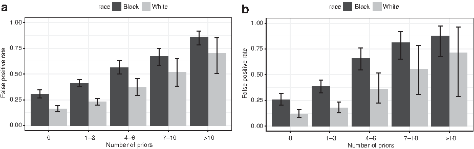
One might expect that differences in FPRs are largely attributable to the subset of defendants who are charged with more serious offenses and who have a larger number of prior arrests/convictions. Although it is true that the FPRs within both racial groups are higher for defendants with worse criminal histories, considerable between-group differences in these error rates persist across low prior count subgroups. Figure 2 shows plots of FPRs across different ranges of prior count for all defendants and also for the subset charged with a misdemeanor offense, which is the lowest severity criminal offense category. As one can see, differences in FPRs between black defendants and white defendants persist across prior record subgroups.
False positive rates across prior record count. Plot is based on assessing a defendant as “high risk” if his or her COMPAS decile score is \documentclass{aastex}\usepackage{amsbsy}\usepackage{amsfonts}\usepackage{amssymb}\usepackage{bm}\usepackage{mathrsfs}\usepackage{pifont}\usepackage{stmaryrd}\usepackage{textcomp}\usepackage{portland, xspace}\usepackage{amsmath, amsxtra}\usepackage{upgreek}\pagestyle{empty}\DeclareMathSizes{10}{9}{7}{6}\begin{document}
$$> {s_{{ \rm{HR}}}} = 4$$
\end{document}. Error bars represent 95% confidence intervals. (a) All defendants. (b) Defendants charged with a Misdemeanor offense.
In general, all of the theoretical results presented in this section extend to the setting wherein we further condition on the covariates X. The main difference is that all classification metrics would need to be evaluated conditional on X. For instance, assuming that \documentclass{aastex}\usepackage{amsbsy}\usepackage{amsfonts}\usepackage{amssymb}\usepackage{bm}\usepackage{mathrsfs}\usepackage{pifont}\usepackage{stmaryrd}\usepackage{textcomp}\usepackage{portland, xspace}\usepackage{amsmath, amsxtra}\usepackage{upgreek}\pagestyle{empty}\DeclareMathSizes{10}{9}{7}{6}\begin{document}
$${t_{{ \rm{min}}}}$$
\end{document} and \documentclass{aastex}\usepackage{amsbsy}\usepackage{amsfonts}\usepackage{amssymb}\usepackage{bm}\usepackage{mathrsfs}\usepackage{pifont}\usepackage{stmaryrd}\usepackage{textcomp}\usepackage{portland, xspace}\usepackage{amsmath, amsxtra}\usepackage{upgreek}\pagestyle{empty}\DeclareMathSizes{10}{9}{7}{6}\begin{document}
$${t_{{ \rm{max}}}}$$
\end{document} are constant on a set \documentclass{aastex}\usepackage{amsbsy}\usepackage{amsfonts}\usepackage{amssymb}\usepackage{bm}\usepackage{mathrsfs}\usepackage{pifont}\usepackage{stmaryrd}\usepackage{textcomp}\usepackage{portland, xspace}\usepackage{amsmath, amsxtra}\usepackage{upgreek}\pagestyle{empty}\DeclareMathSizes{10}{9}{7}{6}\begin{document}
$${ \cal X} ,$$
\end{document} Corollary 3.1 would say that the difference in average penalty under the MinMax policy among nonrecidivists for whom \documentclass{aastex}\usepackage{amsbsy}\usepackage{amsfonts}\usepackage{amssymb}\usepackage{bm}\usepackage{mathrsfs}\usepackage{pifont}\usepackage{stmaryrd}\usepackage{textcomp}\usepackage{portland, xspace}\usepackage{amsmath, amsxtra}\usepackage{upgreek}\pagestyle{empty}\DeclareMathSizes{10}{9}{7}{6}\begin{document}
$$X \in { \cal X}$$
\end{document} is given by
\documentclass{aastex}\usepackage{amsbsy}\usepackage{amsfonts}\usepackage{amssymb}\usepackage{bm}\usepackage{mathrsfs}\usepackage{pifont}\usepackage{stmaryrd}\usepackage{textcomp}\usepackage{portland, xspace}\usepackage{amsmath, amsxtra}\usepackage{upgreek}\pagestyle{empty}\DeclareMathSizes{10}{9}{7}{6}\begin{document}
\begin{align*}
\Delta = ( {t_{{ \rm{max}}}} - {t_{{ \rm{min}}}} ) \left( {{ \rm{FP}}{{ \rm{R}}_b} ( { \cal X} ) - { \rm{FP}}{{ \rm{R}}_w} ( { \cal X} ) } \right). \tag{3.4}
\end{align*}
\end{document}\documentclass{aastex}\usepackage{amsbsy}\usepackage{amsfonts}\usepackage{amssymb}\usepackage{bm}\usepackage{mathrsfs}\usepackage{pifont}\usepackage{stmaryrd}\usepackage{textcomp}\usepackage{portland, xspace}\usepackage{amsmath, amsxtra}\usepackage{upgreek}\pagestyle{empty}\DeclareMathSizes{10}{9}{7}{6}\begin{document}
\begin{align*}
\begin{split}\quad & \equiv ( {t_{{ \rm{max}}}} - {t_{{ \rm{min}}}}
) ( { {\mathbb P} ( S > {s_{{ \rm{HR}}}} \vert R = b , Y = 0 , X
\in { \cal X} )} \\ & \quad- {\mathbb P} ( S > {s_{{ \rm{HR}}}}
\vert R = w , Y = 0 , X \in { \cal X} ) ).\end{split}
\tag{3.5}
\end{align*}
\end{document}
The FPRs shown in Figure 2a correspond precisely to the quantities \documentclass{aastex}\usepackage{amsbsy}\usepackage{amsfonts}\usepackage{amssymb}\usepackage{bm}\usepackage{mathrsfs}\usepackage{pifont}\usepackage{stmaryrd}\usepackage{textcomp}\usepackage{portland, xspace}\usepackage{amsmath, amsxtra}\usepackage{upgreek}\pagestyle{empty}\DeclareMathSizes{10}{9}{7}{6}\begin{document}
$${ \rm{FP}}{{ \rm{R}}_r} ( { \cal X} )$$
\end{document} for choices of \documentclass{aastex}\usepackage{amsbsy}\usepackage{amsfonts}\usepackage{amssymb}\usepackage{bm}\usepackage{mathrsfs}\usepackage{pifont}\usepackage{stmaryrd}\usepackage{textcomp}\usepackage{portland, xspace}\usepackage{amsmath, amsxtra}\usepackage{upgreek}\pagestyle{empty}\DeclareMathSizes{10}{9}{7}{6}\begin{document}
$${ \cal X}$$
\end{document} given by different prior record count bins. The leftmost bars correspond to taking \documentclass{aastex}\usepackage{amsbsy}\usepackage{amsfonts}\usepackage{amssymb}\usepackage{bm}\usepackage{mathrsfs}\usepackage{pifont}\usepackage{stmaryrd}\usepackage{textcomp}\usepackage{portland, xspace}\usepackage{amsmath, amsxtra}\usepackage{upgreek}\pagestyle{empty}\DeclareMathSizes{10}{9}{7}{6}\begin{document}
$${ \cal X} = \{ \# { \rm{priors}} = 0 \} $$
\end{document}. Similarly the leftmost bars in Figure 2a correspond to taking \documentclass{aastex}\usepackage{amsbsy}\usepackage{amsfonts}\usepackage{amssymb}\usepackage{bm}\usepackage{mathrsfs}\usepackage{pifont}\usepackage{stmaryrd}\usepackage{textcomp}\usepackage{portland, xspace}\usepackage{amsmath, amsxtra}\usepackage{upgreek}\pagestyle{empty}\DeclareMathSizes{10}{9}{7}{6}\begin{document}
$${ \cal X} = \{ \# { \rm{priors}} = 0 , { \rm{charge_{degree}}} = M \} $$
\end{document}. In Appendix B we present a logistic regression analysis, showing that significant differences in FPRs persist even after adjusting for a number of other recidivism-related covariates.
Connections to measures of differences in distribution
In their analysis of the PCRA instrument, Skeem and Lowenkamp11 remark that some applications of the risk score could create disparate impact because of differences in the score distributions between black and white offenders. To summarize the distributional difference in scores between the two groups, the authors report a Cohen's d of \documentclass{aastex}\usepackage{amsbsy}\usepackage{amsfonts}\usepackage{amssymb}\usepackage{bm}\usepackage{mathrsfs}\usepackage{pifont}\usepackage{stmaryrd}\usepackage{textcomp}\usepackage{portland, xspace}\usepackage{amsmath, amsxtra}\usepackage{upgreek}\pagestyle{empty}\DeclareMathSizes{10}{9}{7}{6}\begin{document}
$$0.34$$
\end{document}, with a corresponding nonoverlap of 13.5%. A natural question to ask is whether the level of disparity in sentence duration, \documentclass{aastex}\usepackage{amsbsy}\usepackage{amsfonts}\usepackage{amssymb}\usepackage{bm}\usepackage{mathrsfs}\usepackage{pifont}\usepackage{stmaryrd}\usepackage{textcomp}\usepackage{portland, xspace}\usepackage{amsmath, amsxtra}\usepackage{upgreek}\pagestyle{empty}\DeclareMathSizes{10}{9}{7}{6}\begin{document}
$$\Delta$$
\end{document}, is in some sense closely related to such measures of distributional difference. With a small generalization of the percentage nonoverlap measure, we can answer this question in the affirmative.
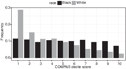
The percentage nonoverlap of two distributions is generally calculated assuming both distributions are normal, and thus has a one-to-one correspondence to Cohen's d.27‡‡ However, as we can see from Figure 3, the COMPAS decile score is far from being normally distributed in either group. A more reasonable way to calculate percentage nonoverlap in such cases is to note that in the Gaussian case percentage nonoverlap is equivalent to the total variation distance. Letting \documentclass{aastex}\usepackage{amsbsy}\usepackage{amsfonts}\usepackage{amssymb}\usepackage{bm}\usepackage{mathrsfs}\usepackage{pifont}\usepackage{stmaryrd}\usepackage{textcomp}\usepackage{portland, xspace}\usepackage{amsmath, amsxtra}\usepackage{upgreek}\pagestyle{empty}\DeclareMathSizes{10}{9}{7}{6}\begin{document}
$${f_{r , y}} ( s )$$
\end{document} denote the score distribution among individuals in group r with recidivism outcome y, one can establish the following sharp bound on \documentclass{aastex}\usepackage{amsbsy}\usepackage{amsfonts}\usepackage{amssymb}\usepackage{bm}\usepackage{mathrsfs}\usepackage{pifont}\usepackage{stmaryrd}\usepackage{textcomp}\usepackage{portland, xspace}\usepackage{amsmath, amsxtra}\usepackage{upgreek}\pagestyle{empty}\DeclareMathSizes{10}{9}{7}{6}\begin{document}
$$\Delta$$
\end{document}.
COMPAS decile score histograms for black and white defendants. Cohen's \documentclass{aastex}\usepackage{amsbsy}\usepackage{amsfonts}\usepackage{amssymb}\usepackage{bm}\usepackage{mathrsfs}\usepackage{pifont}\usepackage{stmaryrd}\usepackage{textcomp}\usepackage{portland, xspace}\usepackage{amsmath, amsxtra}\usepackage{upgreek}\pagestyle{empty}\DeclareMathSizes{10}{9}{7}{6}\begin{document}
$$d = 0.60$$
\end{document}, nonoverlap \documentclass{aastex}\usepackage{amsbsy}\usepackage{amsfonts}\usepackage{amssymb}\usepackage{bm}\usepackage{mathrsfs}\usepackage{pifont}\usepackage{stmaryrd}\usepackage{textcomp}\usepackage{portland, xspace}\usepackage{amsmath, amsxtra}\usepackage{upgreek}\pagestyle{empty}\DeclareMathSizes{10}{9}{7}{6}\begin{document}
$${d_{{ \rm{TV}}}} ( {f_b} , {f_w} ) = 24.5 \%$$
\end{document}.
This result is simple to understand. When there is some nonoverlap between the score distributions for two groups, the worst case scenario is that the nonoverlap is entirely because of mass shifting from scores ≤\documentclass{aastex}\usepackage{amsbsy}\usepackage{amsfonts}\usepackage{amssymb}\usepackage{bm}\usepackage{mathrsfs}\usepackage{pifont}\usepackage{stmaryrd}\usepackage{textcomp}\usepackage{portland, xspace}\usepackage{amsmath, amsxtra}\usepackage{upgreek}\pagestyle{empty}\DeclareMathSizes{10}{9}{7}{6}\begin{document}
$${s_{{ \rm{HR}}}}$$
\end{document} to those >\documentclass{aastex}\usepackage{amsbsy}\usepackage{amsfonts}\usepackage{amssymb}\usepackage{bm}\usepackage{mathrsfs}\usepackage{pifont}\usepackage{stmaryrd}\usepackage{textcomp}\usepackage{portland, xspace}\usepackage{amsmath, amsxtra}\usepackage{upgreek}\pagestyle{empty}\DeclareMathSizes{10}{9}{7}{6}\begin{document}
$${s_{{ \rm{HR}}}}$$
\end{document}. In such cases, the inequality becomes an equality.
Empirical results
In this section we present some empirical results based on two hypothetical sentencing rules: the MinMax rule introduced in the previous section, and the Interpolation rule, which we introduce hereunder. Although the offenders in our data set come from Broward County, Florida, our empirical analysis is modeled on the sentencing guidelines of the State of Pennsylvania.
The penalty ranges \documentclass{aastex}\usepackage{amsbsy}\usepackage{amsfonts}\usepackage{amssymb}\usepackage{bm}\usepackage{mathrsfs}\usepackage{pifont}\usepackage{stmaryrd}\usepackage{textcomp}\usepackage{portland, xspace}\usepackage{amsmath, amsxtra}\usepackage{upgreek}\pagestyle{empty}\DeclareMathSizes{10}{9}{7}{6}\begin{document}
$${t_{{ \rm{min}}}}$$
\end{document} and \documentclass{aastex}\usepackage{amsbsy}\usepackage{amsfonts}\usepackage{amssymb}\usepackage{bm}\usepackage{mathrsfs}\usepackage{pifont}\usepackage{stmaryrd}\usepackage{textcomp}\usepackage{portland, xspace}\usepackage{amsmath, amsxtra}\usepackage{upgreek}\pagestyle{empty}\DeclareMathSizes{10}{9}{7}{6}\begin{document}
$${t_{{ \rm{max}}}}$$
\end{document} are selected by approximately matching each offender's charge degree (M2-F1) to a sentence range in Pennsylvania's Basic Sentencing Matrix (PA Code 303.16). This matrix provides sentence ranges based on the charge degree for the current offense and the defendant's prior record score (0–5+). We do not have enough information in the Broward County data to reliably assign a prior record score for each individual. Our results are based on using the sentencing range corresponding to a prior record score of 1 for all defendants in the data.
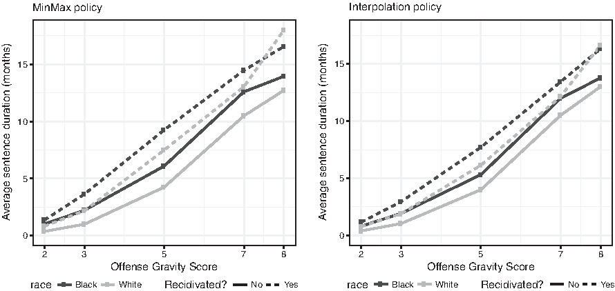
Figure 4 shows the expected sentences for black and white defendants broken down by observed recidivism outcome. The x-axis in these figures is taken to be the offense gravity score, which for the purpose of this analysis is mapped to charge degree as indicated in Table 2.
Average sentences under the hypothetical sentencing policies described in the Empirical Results section. The mapping between the x-axis variable and the offender's charge degree is given in Table 2. For all offense gravity score levels except 8, observed differences in average sentence are statistically significant at the \documentclass{aastex}\usepackage{amsbsy}\usepackage{amsfonts}\usepackage{amssymb}\usepackage{bm}\usepackage{mathrsfs}\usepackage{pifont}\usepackage{stmaryrd}\usepackage{textcomp}\usepackage{portland, xspace}\usepackage{amsmath, amsxtra}\usepackage{upgreek}\pagestyle{empty}\DeclareMathSizes{10}{9}{7}{6}\begin{document}
$$0.01$$
\end{document} level.
Mapping between offense gravity score and charge degree used in the empirical analysis
Offense gravity score
2
3
5
7
8
Charge degree
(M2)
(M1)
(F3)
(F2)
(F1)
Results are shown for both the MinMax policy introduced earlier in this section and the Interpolation policy, which is given by
\documentclass{aastex}\usepackage{amsbsy}\usepackage{amsfonts}\usepackage{amssymb}\usepackage{bm}\usepackage{mathrsfs}\usepackage{pifont}\usepackage{stmaryrd}\usepackage{textcomp}\usepackage{portland, xspace}\usepackage{amsmath, amsxtra}\usepackage{upgreek}\pagestyle{empty}\DeclareMathSizes{10}{9}{7}{6}\begin{document}
\begin{align*}
{ T_ { { \rm { Int } } } } ( s ) = { t_ { { \rm { min } } } } + \frac { { s - 1 } } { 9 } ( { t_ { { \rm { max } } } } - { t_ { { \rm { min } } } } ). \tag { 3.6 }
\end{align*}
\end{document}
Unlike the MinMax policy, which is based on the thresholded score, the Interpolation policy assigns sentences by linearly interpolating between \documentclass{aastex}\usepackage{amsbsy}\usepackage{amsfonts}\usepackage{amssymb}\usepackage{bm}\usepackage{mathrsfs}\usepackage{pifont}\usepackage{stmaryrd}\usepackage{textcomp}\usepackage{portland, xspace}\usepackage{amsmath, amsxtra}\usepackage{upgreek}\pagestyle{empty}\DeclareMathSizes{10}{9}{7}{6}\begin{document}
$${t_{{ \rm{min}}}}$$
\end{document} and \documentclass{aastex}\usepackage{amsbsy}\usepackage{amsfonts}\usepackage{amssymb}\usepackage{bm}\usepackage{mathrsfs}\usepackage{pifont}\usepackage{stmaryrd}\usepackage{textcomp}\usepackage{portland, xspace}\usepackage{amsmath, amsxtra}\usepackage{upgreek}\pagestyle{empty}\DeclareMathSizes{10}{9}{7}{6}\begin{document}
$${t_{{ \rm{max}}}}$$
\end{document} based on the assigned decile score. We see that under both policies, there are consistent trends in the expected sentences. Black defendants are observed to receive higher sentences than white defendants both within the nonrecidivating subgroup and within the recidivating subgroup (except in the F1 charge degree category, wherein sample sizes are small and results are nonsignificant). Since white defendants have higher FNRs and lower FPRs than black defendants, the empirical results are consistent with the theoretical results presented earlier in this section.
Revisiting Predictive Parity
In this section, we revisit the notion of predictive parity and further discuss its implications for general classifiers. We know from Equation (2.6) that when the PPVs are constrained to be equal but the prevalences differ across groups, the FPRs and FNRs cannot both be equal across those groups. Although we have no direct control over recidivism prevalence, we do have some control over the PPV and error rates of our classifiers. At least in principle, we are free to tune our classifiers in any of the following ways:
(i) Allow unequal FNRs to retain equal PPVs and achieve equal FPRs.
(ii) Allow unequal FPRs to retain equal PPVs and achieve equal FNRs.
(iii) Allow unequal PPVs to achieve equal FPRs and FNRs.
Figure 5 helps to put these trade-offs into perspective. From Equation (2.6), we can see that FPR is a linear function of FNR under constraints on PPV and p. This means that if PPV is fixed at a given value, tuning strategy (i) may require a very large increase in \documentclass{aastex}\usepackage{amsbsy}\usepackage{amsfonts}\usepackage{amssymb}\usepackage{bm}\usepackage{mathrsfs}\usepackage{pifont}\usepackage{stmaryrd}\usepackage{textcomp}\usepackage{portland, xspace}\usepackage{amsmath, amsxtra}\usepackage{upgreek}\pagestyle{empty}\DeclareMathSizes{10}{9}{7}{6}\begin{document}
$${ \rm{FNR}}$$
\end{document} to balance FPR. The black line shows feasible combinations of \documentclass{aastex}\usepackage{amsbsy}\usepackage{amsfonts}\usepackage{amssymb}\usepackage{bm}\usepackage{mathrsfs}\usepackage{pifont}\usepackage{stmaryrd}\usepackage{textcomp}\usepackage{portland, xspace}\usepackage{amsmath, amsxtra}\usepackage{upgreek}\pagestyle{empty}\DeclareMathSizes{10}{9}{7}{6}\begin{document}
$$( { \rm{FN}}{{ \rm{R}}_b} , { \rm{FP}}{{ \rm{R}}_b} )$$
\end{document} when \documentclass{aastex}\usepackage{amsbsy}\usepackage{amsfonts}\usepackage{amssymb}\usepackage{bm}\usepackage{mathrsfs}\usepackage{pifont}\usepackage{stmaryrd}\usepackage{textcomp}\usepackage{portland, xspace}\usepackage{amsmath, amsxtra}\usepackage{upgreek}\pagestyle{empty}\DeclareMathSizes{10}{9}{7}{6}\begin{document}
$${ \rm{PP}}{{ \rm{V}}_b}$$
\end{document} is forced to equal the observed value \documentclass{aastex}\usepackage{amsbsy}\usepackage{amsfonts}\usepackage{amssymb}\usepackage{bm}\usepackage{mathrsfs}\usepackage{pifont}\usepackage{stmaryrd}\usepackage{textcomp}\usepackage{portland, xspace}\usepackage{amsmath, amsxtra}\usepackage{upgreek}\pagestyle{empty}\DeclareMathSizes{10}{9}{7}{6}\begin{document}
$${ \rm{PP}}{{ \rm{V}}_w} = 0.591$$
\end{document}. We can see that to get \documentclass{aastex}\usepackage{amsbsy}\usepackage{amsfonts}\usepackage{amssymb}\usepackage{bm}\usepackage{mathrsfs}\usepackage{pifont}\usepackage{stmaryrd}\usepackage{textcomp}\usepackage{portland, xspace}\usepackage{amsmath, amsxtra}\usepackage{upgreek}\pagestyle{empty}\DeclareMathSizes{10}{9}{7}{6}\begin{document}
$${ \rm{FP}}{{ \rm{R}}_b}$$
\end{document} to match \documentclass{aastex}\usepackage{amsbsy}\usepackage{amsfonts}\usepackage{amssymb}\usepackage{bm}\usepackage{mathrsfs}\usepackage{pifont}\usepackage{stmaryrd}\usepackage{textcomp}\usepackage{portland, xspace}\usepackage{amsmath, amsxtra}\usepackage{upgreek}\pagestyle{empty}\DeclareMathSizes{10}{9}{7}{6}\begin{document}
$${ \rm{FP}}{{ \rm{R}}_w}$$
\end{document}, we would need to increase \documentclass{aastex}\usepackage{amsbsy}\usepackage{amsfonts}\usepackage{amssymb}\usepackage{bm}\usepackage{mathrsfs}\usepackage{pifont}\usepackage{stmaryrd}\usepackage{textcomp}\usepackage{portland, xspace}\usepackage{amsmath, amsxtra}\usepackage{upgreek}\pagestyle{empty}\DeclareMathSizes{10}{9}{7}{6}\begin{document}
$${ \rm{FN}}{{ \rm{R}}_b}$$
\end{document} to around \documentclass{aastex}\usepackage{amsbsy}\usepackage{amsfonts}\usepackage{amssymb}\usepackage{bm}\usepackage{mathrsfs}\usepackage{pifont}\usepackage{stmaryrd}\usepackage{textcomp}\usepackage{portland, xspace}\usepackage{amsmath, amsxtra}\usepackage{upgreek}\pagestyle{empty}\DeclareMathSizes{10}{9}{7}{6}\begin{document}
$$0.7$$
\end{document}, which would be a substantial drop in accuracy. In view of Corollaries 3.1 and 3.2, Strategies (i) and (ii) may generally be undesirable because although they reduce disparate impact for one subgroup (e.g., among nonrecidivists), they may increase it in the other.
The two labeled points represent the observed values of (FNR, FPR) for black (B) and white (W) defendants. The broken lighter gray line represents feasible values of (FNR, FPR) for white defendants when the prevalence \documentclass{aastex}\usepackage{amsbsy}\usepackage{amsfonts}\usepackage{amssymb}\usepackage{bm}\usepackage{mathrsfs}\usepackage{pifont}\usepackage{stmaryrd}\usepackage{textcomp}\usepackage{portland, xspace}\usepackage{amsmath, amsxtra}\usepackage{upgreek}\pagestyle{empty}\DeclareMathSizes{10}{9}{7}{6}\begin{document}
$${{ \rm p}_w}$$
\end{document} and \documentclass{aastex}\usepackage{amsbsy}\usepackage{amsfonts}\usepackage{amssymb}\usepackage{bm}\usepackage{mathrsfs}\usepackage{pifont}\usepackage{stmaryrd}\usepackage{textcomp}\usepackage{portland, xspace}\usepackage{amsmath, amsxtra}\usepackage{upgreek}\pagestyle{empty}\DeclareMathSizes{10}{9}{7}{6}\begin{document}
$${ \rm{PP}}{{ \rm{V}}_w}$$
\end{document} are both held fixed at their observed values. The broken dark gray line represents feasible values of \documentclass{aastex}\usepackage{amsbsy}\usepackage{amsfonts}\usepackage{amssymb}\usepackage{bm}\usepackage{mathrsfs}\usepackage{pifont}\usepackage{stmaryrd}\usepackage{textcomp}\usepackage{portland, xspace}\usepackage{amsmath, amsxtra}\usepackage{upgreek}\pagestyle{empty}\DeclareMathSizes{10}{9}{7}{6}\begin{document}
$$( { \rm{FN}}{{ \rm{R}}_b} , { \rm{FP}}{{ \rm{R}}_b} )$$
\end{document} when the prevalence \documentclass{aastex}\usepackage{amsbsy}\usepackage{amsfonts}\usepackage{amssymb}\usepackage{bm}\usepackage{mathrsfs}\usepackage{pifont}\usepackage{stmaryrd}\usepackage{textcomp}\usepackage{portland, xspace}\usepackage{amsmath, amsxtra}\usepackage{upgreek}\pagestyle{empty}\DeclareMathSizes{10}{9}{7}{6}\begin{document}
$${{ \rm p}_b}$$
\end{document} is held fixed at the observed value and \documentclass{aastex}\usepackage{amsbsy}\usepackage{amsfonts}\usepackage{amssymb}\usepackage{bm}\usepackage{mathrsfs}\usepackage{pifont}\usepackage{stmaryrd}\usepackage{textcomp}\usepackage{portland, xspace}\usepackage{amsmath, amsxtra}\usepackage{upgreek}\pagestyle{empty}\DeclareMathSizes{10}{9}{7}{6}\begin{document}
$${ \rm{PP}}{{ \rm{V}}_b}$$
\end{document} is set equal to the observed value of \documentclass{aastex}\usepackage{amsbsy}\usepackage{amsfonts}\usepackage{amssymb}\usepackage{bm}\usepackage{mathrsfs}\usepackage{pifont}\usepackage{stmaryrd}\usepackage{textcomp}\usepackage{portland, xspace}\usepackage{amsmath, amsxtra}\usepackage{upgreek}\pagestyle{empty}\DeclareMathSizes{10}{9}{7}{6}\begin{document}
$${ \rm{PP}}{{ \rm{V}}_w} = 0.591$$
\end{document}. Nested shaded regions correspond to feasible values of \documentclass{aastex}\usepackage{amsbsy}\usepackage{amsfonts}\usepackage{amssymb}\usepackage{bm}\usepackage{mathrsfs}\usepackage{pifont}\usepackage{stmaryrd}\usepackage{textcomp}\usepackage{portland, xspace}\usepackage{amsmath, amsxtra}\usepackage{upgreek}\pagestyle{empty}\DeclareMathSizes{10}{9}{7}{6}\begin{document}
$$( { \rm{FN}}{{ \rm{R}}_b} , { \rm{FP}}{{ \rm{R}}_b} )$$
\end{document} if we allow \documentclass{aastex}\usepackage{amsbsy}\usepackage{amsfonts}\usepackage{amssymb}\usepackage{bm}\usepackage{mathrsfs}\usepackage{pifont}\usepackage{stmaryrd}\usepackage{textcomp}\usepackage{portland, xspace}\usepackage{amsmath, amsxtra}\usepackage{upgreek}\pagestyle{empty}\DeclareMathSizes{10}{9}{7}{6}\begin{document}
$${ \rm{PP}}{{ \rm{V}}_b}$$
\end{document} to vary under the constraint \documentclass{aastex}\usepackage{amsbsy}\usepackage{amsfonts}\usepackage{amssymb}\usepackage{bm}\usepackage{mathrsfs}\usepackage{pifont}\usepackage{stmaryrd}\usepackage{textcomp}\usepackage{portland, xspace}\usepackage{amsmath, amsxtra}\usepackage{upgreek}\pagestyle{empty}\DeclareMathSizes{10}{9}{7}{6}\begin{document}
$$\vert { \rm{PP}}{{ \rm{V}}_b} - 0.591 \vert < \delta$$
\end{document}, with \documentclass{aastex}\usepackage{amsbsy}\usepackage{amsfonts}\usepackage{amssymb}\usepackage{bm}\usepackage{mathrsfs}\usepackage{pifont}\usepackage{stmaryrd}\usepackage{textcomp}\usepackage{portland, xspace}\usepackage{amsmath, amsxtra}\usepackage{upgreek}\pagestyle{empty}\DeclareMathSizes{10}{9}{7}{6}\begin{document}
$$\delta \in \{ 0.05 , 0.1 , 0.125 \} $$
\end{document}. The smaller the \documentclass{aastex}\usepackage{amsbsy}\usepackage{amsfonts}\usepackage{amssymb}\usepackage{bm}\usepackage{mathrsfs}\usepackage{pifont}\usepackage{stmaryrd}\usepackage{textcomp}\usepackage{portland, xspace}\usepackage{amsmath, amsxtra}\usepackage{upgreek}\pagestyle{empty}\DeclareMathSizes{10}{9}{7}{6}\begin{document}
$$\delta$$
\end{document} the smaller the feasible region. FNR, false negative rate; FPR, false positive rate; PPV, positive predictive value.
The preferred approach, at least in some cases, may be to pursue strategy (iii). This amounts to using a score S that does not satisfy predictive parity in the first place, but can also be achieved by allowing the high-risk cutoff \documentclass{aastex}\usepackage{amsbsy}\usepackage{amsfonts}\usepackage{amssymb}\usepackage{bm}\usepackage{mathrsfs}\usepackage{pifont}\usepackage{stmaryrd}\usepackage{textcomp}\usepackage{portland, xspace}\usepackage{amsmath, amsxtra}\usepackage{upgreek}\pagestyle{empty}\DeclareMathSizes{10}{9}{7}{6}\begin{document}
$${s_{{ \rm{HR}} , r}}$$
\end{document} to differ across groups. The shaded regions in Figure 5 show feasible values of \documentclass{aastex}\usepackage{amsbsy}\usepackage{amsfonts}\usepackage{amssymb}\usepackage{bm}\usepackage{mathrsfs}\usepackage{pifont}\usepackage{stmaryrd}\usepackage{textcomp}\usepackage{portland, xspace}\usepackage{amsmath, amsxtra}\usepackage{upgreek}\pagestyle{empty}\DeclareMathSizes{10}{9}{7}{6}\begin{document}
$$( { \rm{FN}}{{ \rm{R}}_b} , { \rm{FP}}{{ \rm{R}}_b} )$$
\end{document} when we allow \documentclass{aastex}\usepackage{amsbsy}\usepackage{amsfonts}\usepackage{amssymb}\usepackage{bm}\usepackage{mathrsfs}\usepackage{pifont}\usepackage{stmaryrd}\usepackage{textcomp}\usepackage{portland, xspace}\usepackage{amsmath, amsxtra}\usepackage{upgreek}\pagestyle{empty}\DeclareMathSizes{10}{9}{7}{6}\begin{document}
$${ \rm{PP}}{{ \rm{V}}_b}$$
\end{document} to be within some \documentclass{aastex}\usepackage{amsbsy}\usepackage{amsfonts}\usepackage{amssymb}\usepackage{bm}\usepackage{mathrsfs}\usepackage{pifont}\usepackage{stmaryrd}\usepackage{textcomp}\usepackage{portland, xspace}\usepackage{amsmath, amsxtra}\usepackage{upgreek}\pagestyle{empty}\DeclareMathSizes{10}{9}{7}{6}\begin{document}
$$\delta$$
\end{document} of the observed value of \documentclass{aastex}\usepackage{amsbsy}\usepackage{amsfonts}\usepackage{amssymb}\usepackage{bm}\usepackage{mathrsfs}\usepackage{pifont}\usepackage{stmaryrd}\usepackage{textcomp}\usepackage{portland, xspace}\usepackage{amsmath, amsxtra}\usepackage{upgreek}\pagestyle{empty}\DeclareMathSizes{10}{9}{7}{6}\begin{document}
$${ \rm{PP}}{{ \rm{V}}_w}$$
\end{document}. We can see that even at small values of \documentclass{aastex}\usepackage{amsbsy}\usepackage{amsfonts}\usepackage{amssymb}\usepackage{bm}\usepackage{mathrsfs}\usepackage{pifont}\usepackage{stmaryrd}\usepackage{textcomp}\usepackage{portland, xspace}\usepackage{amsmath, amsxtra}\usepackage{upgreek}\pagestyle{empty}\DeclareMathSizes{10}{9}{7}{6}\begin{document}
$$\delta$$
\end{document} the feasible region is quite large.
Discussion
The primary contribution of this article was to show how disparate impact can result from the use of a RPI that is known to satisfy the fairness criterion of predictive parity. Our analysis focused on the simple setting wherein a binary risk assessment was used to inform a binary penalty policy. Although all of the formulas have natural analogues in the nonbinary score and penalty setting, we find that many of the salient features are already present in the analysis of the simpler binary–binary problem.
A key limitation of our analysis stems from potential biases in the observed data that may affect our ability to draw valid inferences concerning the fairness of an RPI. Throughout this article, we have implicitly operated under the assumption that the observed recidivism outcome Y is a suitable outcome measure for the purpose of assessing the fairness properties of an RPI. However, the true outcome of interest in this context is reoffense, which is not what we observe. In the latest statistics released by the Federal Bureau of Investigation,28 it is reported that 46% of violent crimes and 19.4% of property crimes were successfully cleared by law enforcement agencies. Many criminal offenders are simply never identified. It is, therefore, possible that a non-negligible fraction of the individuals in our data for whom we observed \documentclass{aastex}\usepackage{amsbsy}\usepackage{amsfonts}\usepackage{amssymb}\usepackage{bm}\usepackage{mathrsfs}\usepackage{pifont}\usepackage{stmaryrd}\usepackage{textcomp}\usepackage{portland, xspace}\usepackage{amsmath, amsxtra}\usepackage{upgreek}\pagestyle{empty}\DeclareMathSizes{10}{9}{7}{6}\begin{document}
$$Y = 0$$
\end{document} did in truth reoffend. If this is indeed the case, and if there are group differences in the rates at which offenders are caught, the findings of empirical fairness assessments may be misleading. Understanding how such forms of data bias affect the ability to assess instruments with respect to different fairness criteria is a subject of our ongoing research efforts.
Conclusion
In closing, we would like to note that there is a large body of literature showing that data-driven risk assessment instruments tend to be more accurate than professional human judgments,29–32 and investigating whether human-driven decisions are themselves prone to exhibiting racial bias.33,34 We should not abandon the data-driven approach on the basis of negative headlines. Rather, we need to work to ensure that the instruments we use appropriately trade-off between the kinds of biases that could lead to disparate impact in the specific contexts in which they are to be applied.
Footnotes
Author Disclosure Statement
No competing financial interests exist.
Cite this article as: Chouldechova A (2017) Fair prediction with disparate impact: A study of bias in recidivism prediction instruments. Big Data 5:2, 153–163, DOI: 10.1089/big.2016.0047.
Appendix A
Proofs
Proof of Proposition 3.1. To simplify notation, we let HR denote the event \documentclass{aastex}\usepackage{amsbsy}\usepackage{amsfonts}\usepackage{amssymb}\usepackage{bm}\usepackage{mathrsfs}\usepackage{pifont}\usepackage{stmaryrd}\usepackage{textcomp}\usepackage{portland, xspace}\usepackage{amsmath, amsxtra}\usepackage{upgreek}\pagestyle{empty}\DeclareMathSizes{10}{9}{7}{6}\begin{document}
$$\{ S > {s_{{ \rm{HR}}}} \} $$
\end{document}.
Proof of Proposition 3.2. By definition of total variation distance, for any event A,
Applying this inequality to Proposition 3.1 with \documentclass{aastex}\usepackage{amsbsy}\usepackage{amsfonts}\usepackage{amssymb}\usepackage{bm}\usepackage{mathrsfs}\usepackage{pifont}\usepackage{stmaryrd}\usepackage{textcomp}\usepackage{portland, xspace}\usepackage{amsmath, amsxtra}\usepackage{upgreek}\pagestyle{empty}\DeclareMathSizes{10}{9}{7}{6}\begin{document}
$$A = \{ {S_c} = { \rm{HR}} \} $$
\end{document} gives
Appendix B
Covariate-adjusted FPRs
In this section we present the results of a logistic regression analysis that we conducted to assess whether the observed differences in FPRs between black and white defendants can be entirely accounted for by other covariates. We find that adjusting for covariates decreases the gap, but it nevertheless remains large and statistically significant.
For the purpose of this analysis, we consider only the subset of defendants who do not recidivate. The outcome variable for the logistic regression is taken to be
where S denotes the COMPAS decile score. In this setup, \documentclass{aastex}\usepackage{amsbsy}\usepackage{amsfonts}\usepackage{amssymb}\usepackage{bm}\usepackage{mathrsfs}\usepackage{pifont}\usepackage{stmaryrd}\usepackage{textcomp}\usepackage{portland, xspace}\usepackage{amsmath, amsxtra}\usepackage{upgreek}\pagestyle{empty}\DeclareMathSizes{10}{9}{7}{6}\begin{document}
$$y = 0$$
\end{document} denotes a True Negative and \documentclass{aastex}\usepackage{amsbsy}\usepackage{amsfonts}\usepackage{amssymb}\usepackage{bm}\usepackage{mathrsfs}\usepackage{pifont}\usepackage{stmaryrd}\usepackage{textcomp}\usepackage{portland, xspace}\usepackage{amsmath, amsxtra}\usepackage{upgreek}\pagestyle{empty}\DeclareMathSizes{10}{9}{7}{6}\begin{document}
$$y = 1$$
\end{document} denotes a False Positive. Statistically significant positive coefficient estimates correspond to variables associated with increased likelihood of false positives.
Appendix Table 1 shows the results of regressing y on race alone. The coefficient of race in this model is large, positive, and statistically significant. Without adjusting for other covariates, the odds that a nonrecidivating black defendant receives a high-risk assessment are \documentclass{aastex}\usepackage{amsbsy}\usepackage{amsfonts}\usepackage{amssymb}\usepackage{bm}\usepackage{mathrsfs}\usepackage{pifont}\usepackage{stmaryrd}\usepackage{textcomp}\usepackage{portland, xspace}\usepackage{amsmath, amsxtra}\usepackage{upgreek}\pagestyle{empty}\DeclareMathSizes{10}{9}{7}{6}\begin{document}
$${e^{0.976}} = 2.6$$
\end{document} times higher than those of a white defendant.
Appendix Table 2 shows the results of regressing y on race, age, gender, number of priors, and charge degree. The coefficient of race is smaller than it was in the unadjusted model, but it is nevertheless large and statistically significant. Even after adjusting for these other factors, the odds that a nonrecidivating black defendant receives a high-risk assessment are \documentclass{aastex}\usepackage{amsbsy}\usepackage{amsfonts}\usepackage{amssymb}\usepackage{bm}\usepackage{mathrsfs}\usepackage{pifont}\usepackage{stmaryrd}\usepackage{textcomp}\usepackage{portland, xspace}\usepackage{amsmath, amsxtra}\usepackage{upgreek}\pagestyle{empty}\DeclareMathSizes{10}{9}{7}{6}\begin{document}
$${e^{0.547}} = 1.72$$
\end{document} times higher than those of a white defendant.
FloresAW, BechtelK, LowenkampCT. False positives, false negatives, and false analyses: A rejoinder to “machine bias: There's software used across the country to predict future criminals. And it's biased against blacks. 2016. Available at: http://www.crj.org/page/-/publications/rejoinder7.11.pdf
SkeemJL, MonahanJ, LowenkampCT. Gender, risk assessment, and sanctioning: The cost of treating women like men. Law Hum Behav. 2016; 40:580–593.
13.
HardtM, PriceE, SrebroN, et al.Equality of opportunity in supervised learning. In: Advances in Neural Information Processing Systems. NIPS, 2016, pp. 3315–3323.
14.
ZliobaiteI.On the relation between accuracy and fairness in binary classification. arXiv preprint arXiv: 1505.05723, 2015.
15.
DworkC, HardtM, PitassiT, et al.Fairness through awareness. In: Proceedings of the 3rd Innovations in Theoretical Computer Science Conference. ACM, 2012, pp. 214–226.
16.
CaldersT, VerwerS. Three naive bayes approaches for discrimination-free classification. Data Mining Knowl Discov. 2010; 210:277–292.
17.
FishB, KunJ, Lelkes ÁD. A confidence-based approach for balancing fairness and accuracy. In: Proceedings of the 2016 SIAM International Conference on Data Mining. SIAM, 2016, pp. 144–152.
18.
RomeiA, RuggieriS. A multidisciplinary survey on discrimination analysis. T Knowl Eng Rev. 2014; 290:582–638.
19.
BarocasS, SelbstAD. Big data's disparate impact. Cal Law Rev. 2016; 104:67–1.
20.
Hannah-MoffatK.Actuarial sentencing: An unsettled? proposition. Justice Quart. 2013; 300:270–296.
21.
SkeemJ.Risk technology in sentencing: Testing the promises and perils (commentary on hannah-moffat, 2011). Justice Quart. 2013; 300:297–303.
22.
MonahanJ, SkeemJL. Risk assessment in criminal sentencing. Annu Rev Clin Psychol. 2016; 12:489–513.
23.
KleinbergJ, MullainathanS, RaghavanM. Inherent trade-offs in the fair determination of risk scores. arXiv preprint arXiv: 1609.05807, 2016.
RitterN.Predicting recidivism risk: New tool in Philadelphia shows great promise. Natl Inst Just J, 271, 2013.
26.
PCS. Validation of risk scale. Technical report, Pennsylvania Commission on Sentencing, 2013.
27.
CohenJ.Statistical power analysis for the behavioral sciences (2nd edition). Mahwah, NJ: Lawrence Erlbaum Associates, 1988.
28.
Uniform crime report: Crime in the UnitedStates, 2015-offenses cleared. U.S. Department of Justice, 2016.
29.
MeehlPE.Clinical versus statistical prediction: A theoretical analysis and a review of the evidence. Minneapolis, MN: University of Minnesota Press, 1954.
30.
DawesRM, FaustD, MeehlPE. Clinical versus actuarial judgment. Science. 1989; 243:1668–1674.
31.
GroveWM, ZaldDH, LebowBS, et al.Clinical versus mechanical prediction: A meta-analysis. Psychol Assess. 2000; 12:1–9.
32.
KleinbergJ, LakkarajuH, LeskovecJ, LudwigJ, MullainathanS. Human decisions and machine predictions. Technical report, National Bureau of Economic Research. 2017.
33.
AnwarS, FangH. Testing for racial prejudice in the parole board release process: Theory and evidence. Technical report, National Bureau of Economic Research. 2012.
34.
SweeneyLT, HaneyC. The influence of race on sentencing: A meta-analytic review of experimental studies. Behav Sci Law. 1992; 100:179–195.