Profit-Based Model Selection for Customer Retention Using Individual Customer Lifetime Values

Abstract

The goal of customer retention campaigns, by design, is to add value and enhance the operational efficiency of businesses. For organizations that strive to retain their customers in saturated, and sometimes fast moving, markets such as the telecommunication and banking industries, implementing customer churn prediction models that perform well and in accordance with the business goals is vital. The expected maximum profit (EMP) measure is tailored toward this problem by taking into account the costs and benefits of a retention campaign and estimating its worth for the organization. Unfortunately, the measure assumes fixed and equal customer lifetime value (CLV) for all customers, which has been shown to not correspond well with reality. In this article, we extend the EMP measure to take into account the variability in the lifetime values of customers, thereby basing it on individual characteristics. We demonstrate how to incorporate the heterogeneity of CLVs when CLVs are known, when their prior distribution is known, and when neither is known. By taking into account individual CLVs, our proposed approach of measuring model performance gives novel insights when deciding on a customer retention campaign. The method is dependent on the characteristics of the customer base as is compliant with modern business analytics and accommodates the data-driven culture that has manifested itself within organizations.

Introduction

In modern business analytics, special attention is given to the personal characteristics of customers, which highlights the data-driven culture that has manifested itself within organizations.¹ Classification problems represent one application of business analytics that exist in both industry and academia. Whether it is credit scoring,² churn prediction,³ or website classification,⁴ the common goal is to build well-performing predictive models that correctly classify as many instances as possible. The consequences of incorrectly classifying instances are not always very severe, but the possibility of large losses for the companies that rely on these models should not be overlooked. When designing a retention campaign for customer churn prediction (CCP), including a customer who does not intend to churn will not affect the company very much, while failing to identify a potential churner, who subsequently leaves the firm, will cause losses. However, not all customers have the same value to the company, and a retention action for some might not be profitable at all. When the companies are selecting a churn prediction model to use for their campaign, it is important to take these concerns into account and base the selection on a model performance measure that is tailored to the situation.⁵

As organizations are concerned about their profit, it is reasonable to choose a performance measure that maximizes the expected profit of the potential retention campaign. The recently proposed state-of-the-art maximum profit (MP)³ and expected maximum profit (EMP)⁵ measures were developed with this objective. The latter measure of binary classifier performance has been adapted for CCP⁵ as well as credit scoring,⁶ in addition to having been incorporated in the construction of the classification model itself⁷ and for feature selection.⁸ In the case of customer churn, the measure takes into account the costs and benefits of the retention campaign, and optimizes the expected profit in addition to giving the fraction of the customer base that should be included in the campaign to achieve that MP. These values are computed using various parameters, such as customer lifetime value (CLV), the cost of contacting a customer, the cost of the retention offer, and the probability that a customer included in the campaign accepts the retention offer. Since this last parameter is typically not known and even difficult to estimate, the EMP models it with a random variable after a beta distribution. The other parameters are, however, assumed to be known. In particular, the CLV is considered fixed and equal for all customers.

CLV has been a popular research topic for some years.⁹ It is defined as the present value of all the future cash flows attributed to a customer's relationship with an organization and offers the advantage to assess the financial value of each customer, with the aim of identifying the most profitable customers and to nurture long-term relationships.¹⁰ However, as has been demonstrated in the literature, CLV is not straightforward to assess.¹¹ Owing to the different types of customer relationships and transaction occasions, CLV needs to be carefully modeled while taking into account the problem setting. In addition, there are both deterministic and stochastic models, which either estimate CLV purely based on historic data or model the various components of CLV using probability distributions.¹² A common and inaccurate assumption that is often made when CLV is estimated concerns the heterogeneity of the customer base.¹³ Although most studies focus on a point estimate of CLV, the literature has recognized the importance of the volatility of CLV. Estimating the variance of the customers' lifetime values is important because the customer base of most companies is by no means uniform, and customers of different levels have different needs, which should be addressed at an individual level for proper customer relationship management.^13,14 The EMP measure, as proposed by Verbraken et al., assumes a fixed and equal CLV for all customers.

In this article, we introduce a new way of incorporating customer heterogeneity in the earlier introduced EMP measure by allowing the CLV to vary on a subject basis. We demonstrate how this can be achieved when individual CLVs are available and—in the case when they are not—how estimates can be obtained. The result is a distribution of EMP values to which we apply bootstrap techniques to generate confidence intervals to help distinguish between good and bad models. We apply our techniques to two real-life data sets and five benchmark data sets using six distinct classification techniques and to demonstrate the usefulness of our approach, compared with the standard EMP measure and the commonly used area under the ROC (receiver operating characteristic) curve (AUC) and top decile lift measures. Since our method explicitly takes into account the variability of the customer base, it has the advantage over the traditional EMP measure to provide a range in performance, which can be beneficial when selecting a model for a retention campaign.

The rest of this article is organized as follows. In the next section, we discuss the theoretical background to our work, including both measuring of classifier performance and the computation of CLV. Subsequently, we present our extension to the EMP measure, which is the main contribution of our article. In the Empirical Evaluation section, we apply the proposed techniques to a collection of data sets and compare the results with other measures. Finally, we discuss the managerial implications of our results, limitations of our study, and opportunities for future research.

Theoretical Background

Measuring model performance

Evaluating the performance of a binary classifier is vital when comparing different models and selecting the best one. Here, we describe the fundamental terminology and methods of this process followed by a description of the more advanced H-measure and EMP measure.

In the case of customer churn, the goal of a classifier is to correctly identify potential churners, and thus assign a label to each customer as churner, denoted here by 0, and nonchurner denoted by 1.⁵ After applying a binary classifier, such as logistic regression (LR), to a customer churn data set, the result is typically a score for each customer in the range [0;1], which can be interpreted as the probability of churning. By determining a cutoff value \documentclass{aastex}\usepackage{amsbsy}\usepackage{amsfonts}\usepackage{amssymb}\usepackage{bm}\usepackage{mathrsfs}\usepackage{pifont}\usepackage{stmaryrd}\usepackage{textcomp}\usepackage{portland, xspace}\usepackage{amsmath, amsxtra}\usepackage{upgreek}\pagestyle{empty}\DeclareMathSizes{10}{9}{7}{6}\begin{document} $$t \in [ 0;1 ]$$ \end{document} , everyone with a score above the cutoff will be considered a predicted churner and everyone with a score below the cutoff a predicted nonchurner. Table 1 gives a confusion matrix resulting from such a classifier, with a cutoff t. In this matrix, N denotes the population size, \documentclass{aastex}\usepackage{amsbsy}\usepackage{amsfonts}\usepackage{amssymb}\usepackage{bm}\usepackage{mathrsfs}\usepackage{pifont}\usepackage{stmaryrd}\usepackage{textcomp}\usepackage{portland, xspace}\usepackage{amsmath, amsxtra}\usepackage{upgreek}\pagestyle{empty}\DeclareMathSizes{10}{9}{7}{6}\begin{document} $${ \pi _0}$$ \end{document} and \documentclass{aastex}\usepackage{amsbsy}\usepackage{amsfonts}\usepackage{amssymb}\usepackage{bm}\usepackage{mathrsfs}\usepackage{pifont}\usepackage{stmaryrd}\usepackage{textcomp}\usepackage{portland, xspace}\usepackage{amsmath, amsxtra}\usepackage{upgreek}\pagestyle{empty}\DeclareMathSizes{10}{9}{7}{6}\begin{document} $${ \pi _1}$$ \end{document} the prior probabilities of classes 0 and 1, and \documentclass{aastex}\usepackage{amsbsy}\usepackage{amsfonts}\usepackage{amssymb}\usepackage{bm}\usepackage{mathrsfs}\usepackage{pifont}\usepackage{stmaryrd}\usepackage{textcomp}\usepackage{portland, xspace}\usepackage{amsmath, amsxtra}\usepackage{upgreek}\pagestyle{empty}\DeclareMathSizes{10}{9}{7}{6}\begin{document} $${F_0} ( t )$$ \end{document} and \documentclass{aastex}\usepackage{amsbsy}\usepackage{amsfonts}\usepackage{amssymb}\usepackage{bm}\usepackage{mathrsfs}\usepackage{pifont}\usepackage{stmaryrd}\usepackage{textcomp}\usepackage{portland, xspace}\usepackage{amsmath, amsxtra}\usepackage{upgreek}\pagestyle{empty}\DeclareMathSizes{10}{9}{7}{6}\begin{document} $${F_1} ( t )$$ \end{document} are the cumulative distribution functions of the scores for both classes. Then, in the matrix, \documentclass{aastex}\usepackage{amsbsy}\usepackage{amsfonts}\usepackage{amssymb}\usepackage{bm}\usepackage{mathrsfs}\usepackage{pifont}\usepackage{stmaryrd}\usepackage{textcomp}\usepackage{portland, xspace}\usepackage{amsmath, amsxtra}\usepackage{upgreek}\pagestyle{empty}\DeclareMathSizes{10}{9}{7}{6}\begin{document} $$N{ \pi _0}{F_0} ( t )$$ \end{document} represents the number of actual churners, which the classifier classifies as churners and \documentclass{aastex}\usepackage{amsbsy}\usepackage{amsfonts}\usepackage{amssymb}\usepackage{bm}\usepackage{mathrsfs}\usepackage{pifont}\usepackage{stmaryrd}\usepackage{textcomp}\usepackage{portland, xspace}\usepackage{amsmath, amsxtra}\usepackage{upgreek}\pagestyle{empty}\DeclareMathSizes{10}{9}{7}{6}\begin{document} $$N{ \pi _1}{F_1} ( t )$$ \end{document} the number of actual nonchurners classified incorrectly as churners. These are also known as true positives and false positives, respectively. When instances are classified correctly or incorrectly, benefits and costs can be associated with the classification, as indicated by b₀, b₁, c₀, and c₁ in the matrix. For example, when a classifier incorrectly classifies a potential churner as a nonchurner, this person will not be included in a retention campaign and will, therefore, inevitably leave, resulting in a loss, or cost, for the company.

Table 1.

Confusion matrix

	Actual class
Predicted class	Class 0	Class 1
Class 0	\documentclass{aastex}\usepackage{amsbsy}\usepackage{amsfonts}\usepackage{amssymb}\usepackage{bm}\usepackage{mathrsfs}\usepackage{pifont}\usepackage{stmaryrd}\usepackage{textcomp}\usepackage{portland, xspace}\usepackage{amsmath, amsxtra}\usepackage{upgreek}\pagestyle{empty}\DeclareMathSizes{10}{9}{7}{6}\begin{document} $$N{ \pi _0}{F_0} ( t )$$ \end{document}	(b₀)	\documentclass{aastex}\usepackage{amsbsy}\usepackage{amsfonts}\usepackage{amssymb}\usepackage{bm}\usepackage{mathrsfs}\usepackage{pifont}\usepackage{stmaryrd}\usepackage{textcomp}\usepackage{portland, xspace}\usepackage{amsmath, amsxtra}\usepackage{upgreek}\pagestyle{empty}\DeclareMathSizes{10}{9}{7}{6}\begin{document} $$N{ \pi _1}{F_1} ( t )$$ \end{document}	(c₁)
Class 1	\documentclass{aastex}\usepackage{amsbsy}\usepackage{amsfonts}\usepackage{amssymb}\usepackage{bm}\usepackage{mathrsfs}\usepackage{pifont}\usepackage{stmaryrd}\usepackage{textcomp}\usepackage{portland, xspace}\usepackage{amsmath, amsxtra}\usepackage{upgreek}\pagestyle{empty}\DeclareMathSizes{10}{9}{7}{6}\begin{document} $$N{ \pi _0} ( 1 - {F_0} ( t ) )$$ \end{document}	(c₀)	\documentclass{aastex}\usepackage{amsbsy}\usepackage{amsfonts}\usepackage{amssymb}\usepackage{bm}\usepackage{mathrsfs}\usepackage{pifont}\usepackage{stmaryrd}\usepackage{textcomp}\usepackage{portland, xspace}\usepackage{amsmath, amsxtra}\usepackage{upgreek}\pagestyle{empty}\DeclareMathSizes{10}{9}{7}{6}\begin{document} $$N{ \pi _1} ( 1 - {F_1} ( t ) )$$ \end{document}	(b₁)

To display classifier performance independent of the cutoff point t, the ROC curve is often used.¹⁵ It graphically displays the trade-off between a classifier's true positive rate (sensitivity) and false positive rate ( \documentclass{aastex}\usepackage{amsbsy}\usepackage{amsfonts}\usepackage{amssymb}\usepackage{bm}\usepackage{mathrsfs}\usepackage{pifont}\usepackage{stmaryrd}\usepackage{textcomp}\usepackage{portland, xspace}\usepackage{amsmath, amsxtra}\usepackage{upgreek}\pagestyle{empty}\DeclareMathSizes{10}{9}{7}{6}\begin{document} $$1 - { \rm{specificity}}$$ \end{document} ). The corresponding AUC is defined as \documentclass{aastex}\usepackage{amsbsy}\usepackage{amsfonts}\usepackage{amssymb}\usepackage{bm}\usepackage{mathrsfs}\usepackage{pifont}\usepackage{stmaryrd}\usepackage{textcomp}\usepackage{portland, xspace}\usepackage{amsmath, amsxtra}\usepackage{upgreek}\pagestyle{empty}\DeclareMathSizes{10}{9}{7}{6}\begin{document} \begin{align*} {\rm{AUC}} = \int {{F_0} ( s ) {f_1} ( s ) ds.} \end{align*} \end{document}

The AUC is a numerical value between 0.5 and 1 that summarizes the ROC curve and is used to compare the performance of different models. A higher AUC value means a better performance of the classifier. Although AUC is very popular for model evaluation, it fails to take into account the cost of misclassification, which can be problematic in the case of class imbalance. In addition, it has been argued that the AUC is an incoherent measure of aggregated classification performance because the probability density that is implicitly assumed when calculating the AUC depends on the empirical score distribution of the classifier itself.¹⁶ However, it is not incoherent when interpreted as a way of evaluating classifier performance in terms of class discrimination.¹⁷

As an alternative, Hand proposed the H-measure, which minimizes the expected loss of a classifier, or the average classification loss, given by the function \documentclass{aastex}\usepackage{amsbsy}\usepackage{amsfonts}\usepackage{amssymb}\usepackage{bm}\usepackage{mathrsfs}\usepackage{pifont}\usepackage{stmaryrd}\usepackage{textcomp}\usepackage{portland, xspace}\usepackage{amsmath, amsxtra}\usepackage{upgreek}\pagestyle{empty}\DeclareMathSizes{10}{9}{7}{6}\begin{document} \begin{align*} Q ( t , c , b ) = b ( c{ \pi _0} ( 1 - {F_0} ( t ) ) + ( 1 - c ) { \pi _1}{F_1} ( t ) ) , \end{align*} \end{document}

where \documentclass{aastex}\usepackage{amsbsy}\usepackage{amsfonts}\usepackage{amssymb}\usepackage{bm}\usepackage{mathrsfs}\usepackage{pifont}\usepackage{stmaryrd}\usepackage{textcomp}\usepackage{portland, xspace}\usepackage{amsmath, amsxtra}\usepackage{upgreek}\pagestyle{empty}\DeclareMathSizes{10}{9}{7}{6}\begin{document} $$b = {c_0} + {c_1}$$ \end{document} and \documentclass{aastex}\usepackage{amsbsy}\usepackage{amsfonts}\usepackage{amssymb}\usepackage{bm}\usepackage{mathrsfs}\usepackage{pifont}\usepackage{stmaryrd}\usepackage{textcomp}\usepackage{portland, xspace}\usepackage{amsmath, amsxtra}\usepackage{upgreek}\pagestyle{empty}\DeclareMathSizes{10}{9}{7}{6}\begin{document} $$c = {c_0} / b$$ \end{document} is the cost ratio.¹⁶ The measure is defined as \documentclass{aastex}\usepackage{amsbsy}\usepackage{amsfonts}\usepackage{amssymb}\usepackage{bm}\usepackage{mathrsfs}\usepackage{pifont}\usepackage{stmaryrd}\usepackage{textcomp}\usepackage{portland, xspace}\usepackage{amsmath, amsxtra}\usepackage{upgreek}\pagestyle{empty}\DeclareMathSizes{10}{9}{7}{6}\begin{document} \begin{align*} H = 1 - { \frac { \int { Q ( T ( c ) ;b , c ) { u_ { \alpha , \beta } } ( c ) dc } } { { \pi _0 } \int_0^ { { \pi _1 } } c { u_ { \alpha , \beta } } ( c ) dc + { \pi _1 } \int_ { { \pi _1 } } ^1 ( 1 - c ) { u_ { \alpha , \beta } } ( c ) dc } } , \end{align*} \end{document}

where \documentclass{aastex}\usepackage{amsbsy}\usepackage{amsfonts}\usepackage{amssymb}\usepackage{bm}\usepackage{mathrsfs}\usepackage{pifont}\usepackage{stmaryrd}\usepackage{textcomp}\usepackage{portland, xspace}\usepackage{amsmath, amsxtra}\usepackage{upgreek}\pagestyle{empty}\DeclareMathSizes{10}{9}{7}{6}\begin{document} $$T ( c )$$ \end{document} is the optimal threshold and \documentclass{aastex}\usepackage{amsbsy}\usepackage{amsfonts}\usepackage{amssymb}\usepackage{bm}\usepackage{mathrsfs}\usepackage{pifont}\usepackage{stmaryrd}\usepackage{textcomp}\usepackage{portland, xspace}\usepackage{amsmath, amsxtra}\usepackage{upgreek}\pagestyle{empty}\DeclareMathSizes{10}{9}{7}{6}\begin{document} $${u_{ \alpha , \beta }}$$ \end{document} is the probability density function of c, assumed here to be a beta distribution with parameters \documentclass{aastex}\usepackage{amsbsy}\usepackage{amsfonts}\usepackage{amssymb}\usepackage{bm}\usepackage{mathrsfs}\usepackage{pifont}\usepackage{stmaryrd}\usepackage{textcomp}\usepackage{portland, xspace}\usepackage{amsmath, amsxtra}\usepackage{upgreek}\pagestyle{empty}\DeclareMathSizes{10}{9}{7}{6}\begin{document} $$\alpha$$ \end{document} and \documentclass{aastex}\usepackage{amsbsy}\usepackage{amsfonts}\usepackage{amssymb}\usepackage{bm}\usepackage{mathrsfs}\usepackage{pifont}\usepackage{stmaryrd}\usepackage{textcomp}\usepackage{portland, xspace}\usepackage{amsmath, amsxtra}\usepackage{upgreek}\pagestyle{empty}\DeclareMathSizes{10}{9}{7}{6}\begin{document} $$\beta$$ \end{document} .*

In the case of building churn prediction models, companies tend to be more concerned about profits than losses. Therefore, Verbeke et al.³ proposed the MP measure as an alternative to the loss minimizing H-measure. The expression for the profit of a retention campaign originates from Neslin et al.¹⁹ and is given by \documentclass{aastex}\usepackage{amsbsy}\usepackage{amsfonts}\usepackage{amssymb}\usepackage{bm}\usepackage{mathrsfs}\usepackage{pifont}\usepackage{stmaryrd}\usepackage{textcomp}\usepackage{portland, xspace}\usepackage{amsmath, amsxtra}\usepackage{upgreek}\pagestyle{empty}\DeclareMathSizes{10}{9}{7}{6}\begin{document} \begin{align*} { \rm{Profit}} = N \eta [ ( \gamma \cdot { \rm{CLV}} + d ( 1 - \gamma ) ) { \pi _0}{ \rm{ \lambda }} - d - f ] - A. \tag{1} \end{align*} \end{document}

This equation describes the profit of a retention campaign based on the flow of customers from and to the customer base, taking into account the fraction of churners ( \documentclass{aastex}\usepackage{amsbsy}\usepackage{amsfonts}\usepackage{amssymb}\usepackage{bm}\usepackage{mathrsfs}\usepackage{pifont}\usepackage{stmaryrd}\usepackage{textcomp}\usepackage{portland, xspace}\usepackage{amsmath, amsxtra}\usepackage{upgreek}\pagestyle{empty}\DeclareMathSizes{10}{9}{7}{6}\begin{document} $${ \rm{ \lambda }}$$ \end{document} ) within the targeted fraction of customers ( \documentclass{aastex}\usepackage{amsbsy}\usepackage{amsfonts}\usepackage{amssymb}\usepackage{bm}\usepackage{mathrsfs}\usepackage{pifont}\usepackage{stmaryrd}\usepackage{textcomp}\usepackage{portland, xspace}\usepackage{amsmath, amsxtra}\usepackage{upgreek}\pagestyle{empty}\DeclareMathSizes{10}{9}{7}{6}\begin{document} $$\eta$$ \end{document} ), the cost of contacting them (f) and offering them a retention offer (d), the fraction of would-be churners who accept the offer ( \documentclass{aastex}\usepackage{amsbsy}\usepackage{amsfonts}\usepackage{amssymb}\usepackage{bm}\usepackage{mathrsfs}\usepackage{pifont}\usepackage{stmaryrd}\usepackage{textcomp}\usepackage{portland, xspace}\usepackage{amsmath, amsxtra}\usepackage{upgreek}\pagestyle{empty}\DeclareMathSizes{10}{9}{7}{6}\begin{document} $$\gamma$$ \end{document} ), and the resulting gain in CLV. The probability that the retention offer has a negative effect is considered negligible. Finally, N is the total number of customers and A the fixed administrative costs. Putting this equation into perspective with the average classification profit of a classifier results in a function of the classification threshold t \documentclass{aastex}\usepackage{amsbsy}\usepackage{amsfonts}\usepackage{amssymb}\usepackage{bm}\usepackage{mathrsfs}\usepackage{pifont}\usepackage{stmaryrd}\usepackage{textcomp}\usepackage{portland, xspace}\usepackage{amsmath, amsxtra}\usepackage{upgreek}\pagestyle{empty}\DeclareMathSizes{10}{9}{7}{6}\begin{document} \begin{align*} P ( t;{b_0} , {c_0} , {b_1} , {c_1} ) = {b_0}{ \pi _0}{F_0} ( t ) + {b_1}{ \pi _1} ( 1 - {F_1} ( t ) ) \\ - {c_0}{ \pi _0} ( 1 - {F_0} ( t ) ) - {c_1}{ \pi _1}{F_1} ( t ). \end{align*} \end{document}

Assuming that \documentclass{aastex}\usepackage{amsbsy}\usepackage{amsfonts}\usepackage{amssymb}\usepackage{bm}\usepackage{mathrsfs}\usepackage{pifont}\usepackage{stmaryrd}\usepackage{textcomp}\usepackage{portland, xspace}\usepackage{amsmath, amsxtra}\usepackage{upgreek}\pagestyle{empty}\DeclareMathSizes{10}{9}{7}{6}\begin{document} $$\eta$$ \end{document} and \documentclass{aastex}\usepackage{amsbsy}\usepackage{amsfonts}\usepackage{amssymb}\usepackage{bm}\usepackage{mathrsfs}\usepackage{pifont}\usepackage{stmaryrd}\usepackage{textcomp}\usepackage{portland, xspace}\usepackage{amsmath, amsxtra}\usepackage{upgreek}\pagestyle{empty}\DeclareMathSizes{10}{9}{7}{6}\begin{document} $$\lambda$$ \end{document} depend on t, they can be expressed as \documentclass{aastex}\usepackage{amsbsy}\usepackage{amsfonts}\usepackage{amssymb}\usepackage{bm}\usepackage{mathrsfs}\usepackage{pifont}\usepackage{stmaryrd}\usepackage{textcomp}\usepackage{portland, xspace}\usepackage{amsmath, amsxtra}\usepackage{upgreek}\pagestyle{empty}\DeclareMathSizes{10}{9}{7}{6}\begin{document} \begin{align*} \eta ( t ) = { \pi _0 } { F_0 } ( t ) + { \pi _1 } { F_1 } ( t ) \quad { \rm { and } } \quad { \rm { \lambda } } ( t ) = { \frac { { F_0 } ( t ) } { { \pi _0 } { F_0 } ( t ) + { \pi _1 } { F_1 } ( t ) } } , \end{align*} \end{document}

and neglecting A leads to the average classification profit of a classifier for customer churn \documentclass{aastex}\usepackage{amsbsy}\usepackage{amsfonts}\usepackage{amssymb}\usepackage{bm}\usepackage{mathrsfs}\usepackage{pifont}\usepackage{stmaryrd}\usepackage{textcomp}\usepackage{portland, xspace}\usepackage{amsmath, amsxtra}\usepackage{upgreek}\pagestyle{empty}\DeclareMathSizes{10}{9}{7}{6}\begin{document} \begin{align*} {P_C} ( t; \eta , { \rm{CLV}} , d , f ) = ( \gamma ( { \rm{CLV}} - d ) - f ) { \pi _0}{F_0} ( t ) \\ - ( d + f ) { \pi _1}{F_1} ( t ) , \end{align*} \end{document}

which means that \documentclass{aastex}\usepackage{amsbsy}\usepackage{amsfonts}\usepackage{amssymb}\usepackage{bm}\usepackage{mathrsfs}\usepackage{pifont}\usepackage{stmaryrd}\usepackage{textcomp}\usepackage{portland, xspace}\usepackage{amsmath, amsxtra}\usepackage{upgreek}\pagestyle{empty}\DeclareMathSizes{10}{9}{7}{6}\begin{document} $${b_0} = \gamma ( { \rm{CLV}} - d ) - f$$ \end{document} and \documentclass{aastex}\usepackage{amsbsy}\usepackage{amsfonts}\usepackage{amssymb}\usepackage{bm}\usepackage{mathrsfs}\usepackage{pifont}\usepackage{stmaryrd}\usepackage{textcomp}\usepackage{portland, xspace}\usepackage{amsmath, amsxtra}\usepackage{upgreek}\pagestyle{empty}\DeclareMathSizes{10}{9}{7}{6}\begin{document} $${c_1} = ( d + f )$$ \end{document} . A threshold for classification can then be selected so that profit is maximized \documentclass{aastex}\usepackage{amsbsy}\usepackage{amsfonts}\usepackage{amssymb}\usepackage{bm}\usepackage{mathrsfs}\usepackage{pifont}\usepackage{stmaryrd}\usepackage{textcomp}\usepackage{portland, xspace}\usepackage{amsmath, amsxtra}\usepackage{upgreek}\pagestyle{empty}\DeclareMathSizes{10}{9}{7}{6}\begin{document} \begin{align*} {t_{opt}} = argma{x_t}{P_C} ( t; \eta , { \rm{CLV}} , d , f ). \end{align*} \end{document}

Verbraken et al. assumed that all the parameters could be estimated, except \documentclass{aastex}\usepackage{amsbsy}\usepackage{amsfonts}\usepackage{amssymb}\usepackage{bm}\usepackage{mathrsfs}\usepackage{pifont}\usepackage{stmaryrd}\usepackage{textcomp}\usepackage{portland, xspace}\usepackage{amsmath, amsxtra}\usepackage{upgreek}\pagestyle{empty}\DeclareMathSizes{10}{9}{7}{6}\begin{document} $$\gamma$$ \end{document} , which is considered a random variable after a beta distribution with parameters \documentclass{aastex}\usepackage{amsbsy}\usepackage{amsfonts}\usepackage{amssymb}\usepackage{bm}\usepackage{mathrsfs}\usepackage{pifont}\usepackage{stmaryrd}\usepackage{textcomp}\usepackage{portland, xspace}\usepackage{amsmath, amsxtra}\usepackage{upgreek}\pagestyle{empty}\DeclareMathSizes{10}{9}{7}{6}\begin{document} $$\alpha$$ \end{document} and \documentclass{aastex}\usepackage{amsbsy}\usepackage{amsfonts}\usepackage{amssymb}\usepackage{bm}\usepackage{mathrsfs}\usepackage{pifont}\usepackage{stmaryrd}\usepackage{textcomp}\usepackage{portland, xspace}\usepackage{amsmath, amsxtra}\usepackage{upgreek}\pagestyle{empty}\DeclareMathSizes{10}{9}{7}{6}\begin{document} $$\beta$$ \end{document} , leading to the following equation for the EMP: \documentclass{aastex}\usepackage{amsbsy}\usepackage{amsfonts}\usepackage{amssymb}\usepackage{bm}\usepackage{mathrsfs}\usepackage{pifont}\usepackage{stmaryrd}\usepackage{textcomp}\usepackage{portland, xspace}\usepackage{amsmath, amsxtra}\usepackage{upgreek}\pagestyle{empty}\DeclareMathSizes{10}{9}{7}{6}\begin{document} \begin{align*} { \rm{EMP}} = \int_ \gamma {P_C} ( {t_{opt}} ( \gamma ) ; \eta , { \rm{CLV}} , d , f ) {u_{ \alpha , \beta }} ( \gamma ) d \gamma. \end{align*} \end{document}

The value of EMP can be computed using an empirical convex hull.^5,16 Finally, based on these calculations, the expected profit maximizing fraction for customer churn is given by \documentclass{aastex}\usepackage{amsbsy}\usepackage{amsfonts}\usepackage{amssymb}\usepackage{bm}\usepackage{mathrsfs}\usepackage{pifont}\usepackage{stmaryrd}\usepackage{textcomp}\usepackage{portland, xspace}\usepackage{amsmath, amsxtra}\usepackage{upgreek}\pagestyle{empty}\DeclareMathSizes{10}{9}{7}{6}\begin{document} \begin{align*} { \eta _{opt}} = \int_ \gamma { \pi _0}{F_0} ( {t_{opt}} ( \gamma ) ) + { \pi _1}{F_1} ( {t_{opt}} ( \gamma ) ) {u_{ \alpha , \beta }} ( \gamma ) d \gamma , \end{align*} \end{document}

and represents the optimal fraction of the customer base that should be targeted in the campaign to achieve the EMP. The fraction is an advantageous side product of the EMP measure, since a cutoff does not have to be determined explicitly. We refer to the MP measure as the standard EMP.

The last performance measure we apply when evaluating our models is the top decile lift.¹⁸ It is commonly used for customer churn models as it compares the ratio of churners in the 10% of customers with the highest predicted probabilities to the ratio of churners in the actual customer base. Thereby, it represents how much better a prediction model is at identifying churners, compared with a random sample of customers.

Customer lifetime value

CLV, defined as the net present value of the cash flows attributed to the relationship with a customer, is a popular research topic as well as being important in the industry.^10,12,20 One of the first general overviews of the CLV literature identified three categories of CLV research directions, namely development of models for calculating CLV, models of customer base analysis, and normative models of CLV, which are mostly used to understand the issues with CLV.²¹ Most studies mainly distinguish between deterministic and probabilistic models, making a point of the former being more suitable for individual calculations, whereas the latter are more adequate for estimating CLV at the cohort level, because they take into account the heterogeneity of the customer base as a whole.²²

Aside from the modeling approach, the customer base is generally regarded as having two dimensions, the type of contract and transaction occasions. The first dimension describes the relationship with the customer, which is either contractual or noncontractual. An example of the first is a customer who has an account in a bank or a telecommunication customer with a fixed contract. Noncontractual relationships are, for example, a customer of a supermarket. The second dimension is the time of purchase, which can be either discrete or continuous. This is illustrated with examples given in Table 2. Each of these settings requires a different modeling approach.

Table 2.

The two dimensions of the customer base

	Transaction occasions
Type of relationship	Discrete	Continuous
Contractual	Magazine subscriptions	Credit card, mobile phone
Noncontractual	Events attendance	Mobile phone, retail purchases

There are numerous challenges of computing and using CLV, with many issues and various components that affect those issues.¹¹ When CLV is computed, it is often assumed that the customer base is homogeneous, which has been shown to be invalid.^22,23 Although most studies focus on estimating the mean value of CLV, it is widely acknowledged in the literature that the variance of CLV is more important.^12,24 To account for this, McCarthy et al.¹⁴ proposed a novel way to derive, predict, and validate the variance of CLV using a combination of stochastic models.

Applications where customers are assumed permanently lost once they terminate their relationship with a company are called “lost for good.” Alternatively, “always a share” scenarios assume that customers, who typically do business with multiple organizations, yet always stay with the firm to a certain extent.²⁵ Gupta et al.¹² presented a universal expression for computing the “lost for good” CLV in terms of the price p_t paid by the customer at time t, the cost c_t of servicing the customer at time t, the discount rate r, the probability r_t of a customer being alive at time t, the acquisition cost AC, and the time horizon T with \documentclass{aastex}\usepackage{amsbsy}\usepackage{amsfonts}\usepackage{amssymb}\usepackage{bm}\usepackage{mathrsfs}\usepackage{pifont}\usepackage{stmaryrd}\usepackage{textcomp}\usepackage{portland, xspace}\usepackage{amsmath, amsxtra}\usepackage{upgreek}\pagestyle{empty}\DeclareMathSizes{10}{9}{7}{6}\begin{document} \begin{align*} { \rm { CLV } } = { \sum \limits_ { t = 0 } ^T } { \frac { ( { p_t } - { c_t } ) { r_t } } { { { ( 1 + r ) } ^t } } } - AC. \end{align*} \end{document}

This expression can be used to compute CLV for both types of relationships, and transaction occasions, and its components can be modeled with both deterministic and stochastic approaches. Multiple derivations exist, where the expression has been simplified and the different components computed in various ways. However, in practice, the most common way to compute CLV is by means of recency-frequency-monetary (RFM) variables.

The type of customer base we consider in this study is contractual and continuous and the relationship is furthermore viewed as “lost-for-good.” Therefore, in the empirical evaluation of this article, CLV is computed in a similar manner as in Glady et al.⁹ using a deterministic approach. There, CLV of customer i at time t is defined as the sum of cash flows CF \documentclass{aastex}\usepackage{amsbsy}\usepackage{amsfonts}\usepackage{amssymb}\usepackage{bm}\usepackage{mathrsfs}\usepackage{pifont}\usepackage{stmaryrd}\usepackage{textcomp}\usepackage{portland, xspace}\usepackage{amsmath, amsxtra}\usepackage{upgreek}\pagestyle{empty}\DeclareMathSizes{10}{9}{7}{6}\begin{document} \begin{align*} { \rm { CL } } { { \rm { V } } _ { i , t } } = \sum \limits_ { k = 1 } ^h \sum \limits_ { j = 1 } ^q \frac { 1 } { { { { ( 1 + r ) } ^k } } } { \rm { C } } { { \rm { F } } _ { i , j , t + h } } , \tag { 2 } \end{align*} \end{document}

where r is the discounting factor, h the time horizon for which CLV is calculated, q the number of products that contribute to the final value, and the net cash flow \documentclass{aastex}\usepackage{amsbsy}\usepackage{amsfonts}\usepackage{amssymb}\usepackage{bm}\usepackage{mathrsfs}\usepackage{pifont}\usepackage{stmaryrd}\usepackage{textcomp}\usepackage{portland, xspace}\usepackage{amsmath, amsxtra}\usepackage{upgreek}\pagestyle{empty}\DeclareMathSizes{10}{9}{7}{6}\begin{document} $${ \rm{C}}{{ \rm{F}}_{i , j , t}}$$ \end{document} of product j belonging to customer i at time t is given by \documentclass{aastex}\usepackage{amsbsy}\usepackage{amsfonts}\usepackage{amssymb}\usepackage{bm}\usepackage{mathrsfs}\usepackage{pifont}\usepackage{stmaryrd}\usepackage{textcomp}\usepackage{portland, xspace}\usepackage{amsmath, amsxtra}\usepackage{upgreek}\pagestyle{empty}\DeclareMathSizes{10}{9}{7}{6}\begin{document} \begin{align*} { \rm{C}}{{ \rm{F}}_{i , j , t}} = { \pi _j}{x_{i , j , t}} , \tag{3} \end{align*} \end{document}

Modeling Variable EMP

Incorporating the heterogeneity of CLV in the EMP

In the EMP measure, \documentclass{aastex}\usepackage{amsbsy}\usepackage{amsfonts}\usepackage{amssymb}\usepackage{bm}\usepackage{mathrsfs}\usepackage{pifont}\usepackage{stmaryrd}\usepackage{textcomp}\usepackage{portland, xspace}\usepackage{amsmath, amsxtra}\usepackage{upgreek}\pagestyle{empty}\DeclareMathSizes{10}{9}{7}{6}\begin{document} $$\gamma$$ \end{document} represents the fraction of customers who accept the retention offer, but it can also be interpreted as the probability of each customer accepting the offer.⁵ We use the latter understanding of parameter \documentclass{aastex}\usepackage{amsbsy}\usepackage{amsfonts}\usepackage{amssymb}\usepackage{bm}\usepackage{mathrsfs}\usepackage{pifont}\usepackage{stmaryrd}\usepackage{textcomp}\usepackage{portland, xspace}\usepackage{amsmath, amsxtra}\usepackage{upgreek}\pagestyle{empty}\DeclareMathSizes{10}{9}{7}{6}\begin{document} $$\gamma$$ \end{document} to derive a distribution of EMP values. Let \documentclass{aastex}\usepackage{amsbsy}\usepackage{amsfonts}\usepackage{amssymb}\usepackage{bm}\usepackage{mathrsfs}\usepackage{pifont}\usepackage{stmaryrd}\usepackage{textcomp}\usepackage{portland, xspace}\usepackage{amsmath, amsxtra}\usepackage{upgreek}\pagestyle{empty}\DeclareMathSizes{10}{9}{7}{6}\begin{document} $${ \bf CLV} = ( { \rm {CLV}} _{i} ) , i \in \{ 1 \ldots N \} $$ \end{document} be a vector of N lifetime values of customers of a given company. They could be either actual values, obtained by CLV modeling, or sampled from a distribution that is representative of the CLV of the customer base. Rewriting Equation (1) to account for each value of CLV, we obtain \documentclass{aastex}\usepackage{amsbsy}\usepackage{amsfonts}\usepackage{amssymb}\usepackage{bm}\usepackage{mathrsfs}\usepackage{pifont}\usepackage{stmaryrd}\usepackage{textcomp}\usepackage{portland, xspace}\usepackage{amsmath, amsxtra}\usepackage{upgreek}\pagestyle{empty}\DeclareMathSizes{10}{9}{7}{6}\begin{document} \begin{align*} { \rm{Profit}} = \eta \sum \limits_{i = 1}^N [ ( \gamma \cdot { \rm{CL}}{{ \rm{V}}_i} + d ( 1 - \gamma ) ) { \pi _0}{ \rm{ \lambda }} - d - f ] - A. \end{align*} \end{document}

As before, we disregard A and use the same substitution to get the average classification profit \documentclass{aastex}\usepackage{amsbsy}\usepackage{amsfonts}\usepackage{amssymb}\usepackage{bm}\usepackage{mathrsfs}\usepackage{pifont}\usepackage{stmaryrd}\usepackage{textcomp}\usepackage{portland, xspace}\usepackage{amsmath, amsxtra}\usepackage{upgreek}\pagestyle{empty}\DeclareMathSizes{10}{9}{7}{6}\begin{document} \begin{align*} P_C ( t; \eta , { \bf { CLV } } , d , f ) & = \frac { 1 } { N } \sum \limits_ { i = 1 } ^N [( \gamma ( { \rm { CL } } { { \rm { V } } _i } - d ) - f ) { \pi _0 } { F_0 } ( t ) \\\quad - ( d + f ) { \pi_1 } { F_1 } ( t )] \\ & = \frac { 1 } { N } \sum \limits_ { i = 1 } ^N { P_C } ( t; \eta , { \rm { CL } } { { \rm { V } } _i } , d , f ) \\ & = \frac { 1 } { N } \sum \limits_ { i = 1 } ^N { P_ { Ci } } ( t ) , \end{align*} \end{document}

where \documentclass{aastex}\usepackage{amsbsy}\usepackage{amsfonts}\usepackage{amssymb}\usepackage{bm}\usepackage{mathrsfs}\usepackage{pifont}\usepackage{stmaryrd}\usepackage{textcomp}\usepackage{portland, xspace}\usepackage{amsmath, amsxtra}\usepackage{upgreek}\pagestyle{empty}\DeclareMathSizes{10}{9}{7}{6}\begin{document} $${P_{Ci}}$$ \end{document} corresponds to the profit associated with CLV_i. We define \documentclass{aastex}\usepackage{amsbsy}\usepackage{amsfonts}\usepackage{amssymb}\usepackage{bm}\usepackage{mathrsfs}\usepackage{pifont}\usepackage{stmaryrd}\usepackage{textcomp}\usepackage{portland, xspace}\usepackage{amsmath, amsxtra}\usepackage{upgreek}\pagestyle{empty}\DeclareMathSizes{10}{9}{7}{6}\begin{document} $${ \rm {EMP}} _{i}$$ \end{document} for each \documentclass{aastex}\usepackage{amsbsy}\usepackage{amsfonts}\usepackage{amssymb}\usepackage{bm}\usepackage{mathrsfs}\usepackage{pifont}\usepackage{stmaryrd}\usepackage{textcomp}\usepackage{portland, xspace}\usepackage{amsmath, amsxtra}\usepackage{upgreek}\pagestyle{empty}\DeclareMathSizes{10}{9}{7}{6}\begin{document} $$i \in \{ 1 , \ldots , N \} $$ \end{document} \documentclass{aastex}\usepackage{amsbsy}\usepackage{amsfonts}\usepackage{amssymb}\usepackage{bm}\usepackage{mathrsfs}\usepackage{pifont}\usepackage{stmaryrd}\usepackage{textcomp}\usepackage{portland, xspace}\usepackage{amsmath, amsxtra}\usepackage{upgreek}\pagestyle{empty}\DeclareMathSizes{10}{9}{7}{6}\begin{document} \begin{align*} { \rm {EMP}}_{i}: & = \int_ \gamma {P_C} ( t; \eta , {{ \rm{CLV}} _{i}} , d , f ) {u_{ \alpha , \beta }} ( \gamma ) d \gamma \\ & = \int_ \gamma {P_{Ci}} ( t ) {u_{ \alpha , \beta }} ( \gamma ) d \gamma , \end{align*} \end{document}

where t is the optimal threshold as before. Note that in the case of constant CLV, \documentclass{aastex}\usepackage{amsbsy}\usepackage{amsfonts}\usepackage{amssymb}\usepackage{bm}\usepackage{mathrsfs}\usepackage{pifont}\usepackage{stmaryrd}\usepackage{textcomp}\usepackage{portland, xspace}\usepackage{amsmath, amsxtra}\usepackage{upgreek}\pagestyle{empty}\DeclareMathSizes{10}{9}{7}{6}\begin{document} $$EMP = \frac { 1 } { N } \sum \nolimits_ { i = 1 } ^N { \rm { EM P } } _ { i } $$ \end{document} . Just as for the vector of CLV, we obtain a vector of EMP values. Each individual value is not meaningful, since EMP is a measure of overall classifier performance, but to gain further understanding of the classifier's performance, we can study the distribution of the EMP values.

Therefore, we proceed to compute separate EMP values for each instance in the vector of the CLV. Summary statistics of the EMP vector can be explored to gain insights into the customer base. In the following analyses, we compute both mean and median values of the EMP vector to estimate model performance. We refer to this version as \documentclass{aastex}\usepackage{amsbsy}\usepackage{amsfonts}\usepackage{amssymb}\usepackage{bm}\usepackage{mathrsfs}\usepackage{pifont}\usepackage{stmaryrd}\usepackage{textcomp}\usepackage{portland, xspace}\usepackage{amsmath, amsxtra}\usepackage{upgreek}\pagestyle{empty}\DeclareMathSizes{10}{9}{7}{6}\begin{document} $${{ \rm{EMP}}_{vector}}$$ \end{document} .

Estimating the EMP distribution

Estimating CLV each time a churn prediction model needs to be evaluated may not be feasible. However, once the values have been calculated once, there is knowledge about their distribution that can be exploited in subsequent computations of the EMP. To this end, we assume that each CLV is a random variable that follows a beta distribution of the second type, or \documentclass{aastex}\usepackage{amsbsy}\usepackage{amsfonts}\usepackage{amssymb}\usepackage{bm}\usepackage{mathrsfs}\usepackage{pifont}\usepackage{stmaryrd}\usepackage{textcomp}\usepackage{portland, xspace}\usepackage{amsmath, amsxtra}\usepackage{upgreek}\pagestyle{empty}\DeclareMathSizes{10}{9}{7}{6}\begin{document} $${\beta \prime}$$ \end{document} . The \documentclass{aastex}\usepackage{amsbsy}\usepackage{amsfonts}\usepackage{amssymb}\usepackage{bm}\usepackage{mathrsfs}\usepackage{pifont}\usepackage{stmaryrd}\usepackage{textcomp}\usepackage{portland, xspace}\usepackage{amsmath, amsxtra}\usepackage{upgreek}\pagestyle{empty}\DeclareMathSizes{10}{9}{7}{6}\begin{document} $${\beta \prime}$$ \end{document} distribution is an absolutely continuous probability distribution on the positive real line with two shape parameters \documentclass{aastex}\usepackage{amsbsy}\usepackage{amsfonts}\usepackage{amssymb}\usepackage{bm}\usepackage{mathrsfs}\usepackage{pifont}\usepackage{stmaryrd}\usepackage{textcomp}\usepackage{portland, xspace}\usepackage{amsmath, amsxtra}\usepackage{upgreek}\pagestyle{empty}\DeclareMathSizes{10}{9}{7}{6}\begin{document} $$\alpha$$ \end{document} and \documentclass{aastex}\usepackage{amsbsy}\usepackage{amsfonts}\usepackage{amssymb}\usepackage{bm}\usepackage{mathrsfs}\usepackage{pifont}\usepackage{stmaryrd}\usepackage{textcomp}\usepackage{portland, xspace}\usepackage{amsmath, amsxtra}\usepackage{upgreek}\pagestyle{empty}\DeclareMathSizes{10}{9}{7}{6}\begin{document} $$\beta$$ \end{document} , which make it customizable. In addition, it can be long tailed that makes it representative of the behavior of CLV. Alternatively other distributions, such as the Pareto or gamma, could be used.

When the prior distribution of the CLVs is known, the parameters of the distribution can be calculated using either the maximum likelihood method or the method of moments.²⁶ Since the maximum likelihood equations for the \documentclass{aastex}\usepackage{amsbsy}\usepackage{amsfonts}\usepackage{amssymb}\usepackage{bm}\usepackage{mathrsfs}\usepackage{pifont}\usepackage{stmaryrd}\usepackage{textcomp}\usepackage{portland, xspace}\usepackage{amsmath, amsxtra}\usepackage{upgreek}\pagestyle{empty}\DeclareMathSizes{10}{9}{7}{6}\begin{document} $${\beta \prime}$$ \end{document} distribution do not have a closed form, it is computationally difficult to estimate its parameters. Therefore, we use the method of moments, under the assumption that \documentclass{aastex}\usepackage{amsbsy}\usepackage{amsfonts}\usepackage{amssymb}\usepackage{bm}\usepackage{mathrsfs}\usepackage{pifont}\usepackage{stmaryrd}\usepackage{textcomp}\usepackage{portland, xspace}\usepackage{amsmath, amsxtra}\usepackage{upgreek}\pagestyle{empty}\DeclareMathSizes{10}{9}{7}{6}\begin{document} $$\alpha > 1$$ \end{document} and \documentclass{aastex}\usepackage{amsbsy}\usepackage{amsfonts}\usepackage{amssymb}\usepackage{bm}\usepackage{mathrsfs}\usepackage{pifont}\usepackage{stmaryrd}\usepackage{textcomp}\usepackage{portland, xspace}\usepackage{amsmath, amsxtra}\usepackage{upgreek}\pagestyle{empty}\DeclareMathSizes{10}{9}{7}{6}\begin{document} $$\beta > 2$$ \end{document} to have finite first and second moments. In general, if X is a random variable that follows the \documentclass{aastex}\usepackage{amsbsy}\usepackage{amsfonts}\usepackage{amssymb}\usepackage{bm}\usepackage{mathrsfs}\usepackage{pifont}\usepackage{stmaryrd}\usepackage{textcomp}\usepackage{portland, xspace}\usepackage{amsmath, amsxtra}\usepackage{upgreek}\pagestyle{empty}\DeclareMathSizes{10}{9}{7}{6}\begin{document} $${\beta \prime}$$ \end{document} distribution with parameters \documentclass{aastex}\usepackage{amsbsy}\usepackage{amsfonts}\usepackage{amssymb}\usepackage{bm}\usepackage{mathrsfs}\usepackage{pifont}\usepackage{stmaryrd}\usepackage{textcomp}\usepackage{portland, xspace}\usepackage{amsmath, amsxtra}\usepackage{upgreek}\pagestyle{empty}\DeclareMathSizes{10}{9}{7}{6}\begin{document} $$\alpha$$ \end{document} and \documentclass{aastex}\usepackage{amsbsy}\usepackage{amsfonts}\usepackage{amssymb}\usepackage{bm}\usepackage{mathrsfs}\usepackage{pifont}\usepackage{stmaryrd}\usepackage{textcomp}\usepackage{portland, xspace}\usepackage{amsmath, amsxtra}\usepackage{upgreek}\pagestyle{empty}\DeclareMathSizes{10}{9}{7}{6}\begin{document} $$\beta$$ \end{document} , then its first and second moments are \documentclass{aastex}\usepackage{amsbsy}\usepackage{amsfonts}\usepackage{amssymb}\usepackage{bm}\usepackage{mathrsfs}\usepackage{pifont}\usepackage{stmaryrd}\usepackage{textcomp}\usepackage{portland, xspace}\usepackage{amsmath, amsxtra}\usepackage{upgreek}\pagestyle{empty}\DeclareMathSizes{10}{9}{7}{6}\begin{document} \begin{align*} \mu : = E [ X ] = { \alpha \over { \beta - 1}} \quad { \rm{and}} \quad { \sigma ^2}: = Var [ X ] = {{ \alpha ( \alpha + \beta - 1 ) } \over {{{ ( \beta - 1 ) }^2} ( \beta - 2 ) }} , \end{align*} \end{document}

respectively. This system of equations can be solved for \documentclass{aastex}\usepackage{amsbsy}\usepackage{amsfonts}\usepackage{amssymb}\usepackage{bm}\usepackage{mathrsfs}\usepackage{pifont}\usepackage{stmaryrd}\usepackage{textcomp}\usepackage{portland, xspace}\usepackage{amsmath, amsxtra}\usepackage{upgreek}\pagestyle{empty}\DeclareMathSizes{10}{9}{7}{6}\begin{document} $$\alpha$$ \end{document} and \documentclass{aastex}\usepackage{amsbsy}\usepackage{amsfonts}\usepackage{amssymb}\usepackage{bm}\usepackage{mathrsfs}\usepackage{pifont}\usepackage{stmaryrd}\usepackage{textcomp}\usepackage{portland, xspace}\usepackage{amsmath, amsxtra}\usepackage{upgreek}\pagestyle{empty}\DeclareMathSizes{10}{9}{7}{6}\begin{document} $$\beta$$ \end{document} giving \documentclass{aastex}\usepackage{amsbsy}\usepackage{amsfonts}\usepackage{amssymb}\usepackage{bm}\usepackage{mathrsfs}\usepackage{pifont}\usepackage{stmaryrd}\usepackage{textcomp}\usepackage{portland, xspace}\usepackage{amsmath, amsxtra}\usepackage{upgreek}\pagestyle{empty}\DeclareMathSizes{10}{9}{7}{6}\begin{document} \begin{align*} \alpha = \mu ( { \frac { \mu ( \mu + 1 ) } { { \sigma ^2 } } } + 1 ) \quad { \rm { and } } \quad \beta = { \frac { \mu ( \mu + 1 ) } { { \sigma ^2 } } } + 2. \tag { 4 } \end{align*} \end{document}

To obtain a vector of CLV for the customers, we draw a sample of size N from the distribution \documentclass{aastex}\usepackage{amsbsy}\usepackage{amsfonts}\usepackage{amssymb}\usepackage{bm}\usepackage{mathrsfs}\usepackage{pifont}\usepackage{stmaryrd}\usepackage{textcomp}\usepackage{portland, xspace}\usepackage{amsmath, amsxtra}\usepackage{upgreek}\pagestyle{empty}\DeclareMathSizes{10}{9}{7}{6}\begin{document} $$\beta \prime ( \alpha , \beta )$$ \end{document} . This sample represents the customer base as a whole, not each individual in the data set, so N only needs to be large enough. \documentclass{aastex}\usepackage{amsbsy}\usepackage{amsfonts}\usepackage{amssymb}\usepackage{bm}\usepackage{mathrsfs}\usepackage{pifont}\usepackage{stmaryrd}\usepackage{textcomp}\usepackage{portland, xspace}\usepackage{amsmath, amsxtra}\usepackage{upgreek}\pagestyle{empty}\DeclareMathSizes{10}{9}{7}{6}\begin{document} $${ \rm{EM}}{{ \rm{P}}_i}$$ \end{document} is subsequently computed for each instance in the sample resulting in the vector \documentclass{aastex}\usepackage{amsbsy}\usepackage{amsfonts}\usepackage{amssymb}\usepackage{bm}\usepackage{mathrsfs}\usepackage{pifont}\usepackage{stmaryrd}\usepackage{textcomp}\usepackage{portland, xspace}\usepackage{amsmath, amsxtra}\usepackage{upgreek}\pagestyle{empty}\DeclareMathSizes{10}{9}{7}{6}\begin{document} $${\rm{EM}}{{ \rm{P}}_{\beta \prime}}$$ \end{document} , which depends on the \documentclass{aastex}\usepackage{amsbsy}\usepackage{amsfonts}\usepackage{amssymb}\usepackage{bm}\usepackage{mathrsfs}\usepackage{pifont}\usepackage{stmaryrd}\usepackage{textcomp}\usepackage{portland, xspace}\usepackage{amsmath, amsxtra}\usepackage{upgreek}\pagestyle{empty}\DeclareMathSizes{10}{9}{7}{6}\begin{document} $$\beta \prime ( \alpha , \beta )$$ \end{document} distribution, as in the previous subsection, and the mean or median can be used to represent the final estimate.

In addition, bootstrap methods can be used to estimate confidence intervals for the sample statistics of the \documentclass{aastex}\usepackage{amsbsy}\usepackage{amsfonts}\usepackage{amssymb}\usepackage{bm}\usepackage{mathrsfs}\usepackage{pifont}\usepackage{stmaryrd}\usepackage{textcomp}\usepackage{portland, xspace}\usepackage{amsmath, amsxtra}\usepackage{upgreek}\pagestyle{empty}\DeclareMathSizes{10}{9}{7}{6}\begin{document} $${ \rm{EM}}{{ \rm{P}}_{ \beta \prime }}$$ \end{document} vector.²⁷ For example, to find a 95% confidence interval for the mean using the percentile method, B bootstrap samples of size M are drawn from the \documentclass{aastex}\usepackage{amsbsy}\usepackage{amsfonts}\usepackage{amssymb}\usepackage{bm}\usepackage{mathrsfs}\usepackage{pifont}\usepackage{stmaryrd}\usepackage{textcomp}\usepackage{portland, xspace}\usepackage{amsmath, amsxtra}\usepackage{upgreek}\pagestyle{empty}\DeclareMathSizes{10}{9}{7}{6}\begin{document} $${ \rm{EM}}{{ \rm{P}}_{ \beta \prime }}$$ \end{document} vector, and the mean is calculated for each sample. Subsequently, the B mean values are arranged in ascending order, and the elements in positions 0.025B and 0.975B are used to represent the lower and upper bounds of the confidence interval, respectively.

Evaluating CLV of customers correctly can be a time-consuming and difficult task that may not be beneficial when it is only needed to measure the performance of churn prediction models. When an organization knows neither the CLV of their customers nor its prior distribution, it is still possible to make use of the methods we have proposed here. To do so, reliable estimates of parameters \documentclass{aastex}\usepackage{amsbsy}\usepackage{amsfonts}\usepackage{amssymb}\usepackage{bm}\usepackage{mathrsfs}\usepackage{pifont}\usepackage{stmaryrd}\usepackage{textcomp}\usepackage{portland, xspace}\usepackage{amsmath, amsxtra}\usepackage{upgreek}\pagestyle{empty}\DeclareMathSizes{10}{9}{7}{6}\begin{document} $$\alpha$$ \end{document} and \documentclass{aastex}\usepackage{amsbsy}\usepackage{amsfonts}\usepackage{amssymb}\usepackage{bm}\usepackage{mathrsfs}\usepackage{pifont}\usepackage{stmaryrd}\usepackage{textcomp}\usepackage{portland, xspace}\usepackage{amsmath, amsxtra}\usepackage{upgreek}\pagestyle{empty}\DeclareMathSizes{10}{9}{7}{6}\begin{document} $$\beta$$ \end{document} are needed to compute \documentclass{aastex}\usepackage{amsbsy}\usepackage{amsfonts}\usepackage{amssymb}\usepackage{bm}\usepackage{mathrsfs}\usepackage{pifont}\usepackage{stmaryrd}\usepackage{textcomp}\usepackage{portland, xspace}\usepackage{amsmath, amsxtra}\usepackage{upgreek}\pagestyle{empty}\DeclareMathSizes{10}{9}{7}{6}\begin{document} $${ \rm{EM}}{{ \rm{P}}_{ \beta \prime }}$$ \end{document} .

Empirical Evaluation

Data sets and CCP modeling

We demonstrate the usage and benefits of our new approach for churn prediction. Table 3 provides a summary of the data sets that we use in our experiments. The first data set (Bank) was provided by a retail bank in Belgium. It spans 3 years of information about the usage of products and services for >0.5 million customers, aggregated at a monthly level. Being rich in the number of features, this data set offers a high potential for accurate estimation of CLV of the customers. In addition, knowledge of actual churners and their churn dates is available.

Table 3.

Data sets

ID	Source	Region	Type	Observations	Features	Churn %
Bank	Operator	Europe	Bank	530,000	264	1.37
Telco	Operator	Europe	Telco	1,200,000	24	1.54
D1	Duke	North America	Telco	12,500	11	39.31
D2	Duke	North America	Telco	6000	39	34.27
D3	Operator	South America	Telco	100,000	50	49.56
D4	Operator	Asia	Telco	13,600	16	22.59
D5	UCI		Telco	5000	20	14.14

The second data set (Telco) comes from a telecommunications company in Belgium. It consists of both customer information, such as demographics, usage, and handset data, and call detail records (CDRs) spanning 6 months for >1 million customers with postpaid contracts. The CDRs, which are logs of phone call traffic used for billing purposes, are used in the estimation of the CLV. This data set has a similar churn rate as the Bank data set, with a high class imbalance.

The remaining five data sets are publicly available and have been used in a number of studies.^3,28 They are both limited in number of observations and features but are included here to demonstrate how our method can be used when CLV is not computable.

For the two real-life data sets, we build churn prediction models following standard methods²⁹ using the binary classifiers LR, decision trees (DTs), and random forests (RFs). These classifiers were chosen because of their popularity in both academia and industry.⁵ LR and DTs are intuitive and easy to interpret and are, therefore, held in high regards, especially in fields where black box models are not feasible. RFs have been shown to be very powerful when it comes to accurate predictions, but being an ensemble of DTs, it is difficult to comprehend the underlying model.⁶ In addition, we use extreme gradient boosting (XGB), artificial neural networks (NN), and support vector machines (SVMs) with radial basis function kernels to predict churn in the data sets D1–D5, to further evaluate our proposed approach. These are all powerful techniques that have been successfully used in the literature to predict churn.^31–33

Except for the Bank data set, the other data sets were randomly split into training set with 70% of the observations and a validation set with the remaining 30% of observations. The Telco data set spans 6 months, and the first 3 months of the data were viewed as the historical information about the customers and used as attributes to predict churn in the last 3 months. Because of the long timeframe of the Bank data set, the first 1.5 years was used for training and the last 1.5 years for validation, resulting in an out-of-time experimental setup. When applicable, models were trained using 10-fold cross-validation on the training set to tune parameters, and subsequently evaluated by applying the final models to the validation sets.

To evaluate model performance, we use AUC, H-measure, top decile lift, and EMP, with default values for the parameters, that is, CLV = €200, d = €10, f = €1, \documentclass{aastex}\usepackage{amsbsy}\usepackage{amsfonts}\usepackage{amssymb}\usepackage{bm}\usepackage{mathrsfs}\usepackage{pifont}\usepackage{stmaryrd}\usepackage{textcomp}\usepackage{portland, xspace}\usepackage{amsmath, amsxtra}\usepackage{upgreek}\pagestyle{empty}\DeclareMathSizes{10}{9}{7}{6}\begin{document} $$\alpha = 6$$ \end{document} , and \documentclass{aastex}\usepackage{amsbsy}\usepackage{amsfonts}\usepackage{amssymb}\usepackage{bm}\usepackage{mathrsfs}\usepackage{pifont}\usepackage{stmaryrd}\usepackage{textcomp}\usepackage{portland, xspace}\usepackage{amsmath, amsxtra}\usepackage{upgreek}\pagestyle{empty}\DeclareMathSizes{10}{9}{7}{6}\begin{document} $$\beta = 14$$ \end{document} .

Figure 1 shows an overview of each step of the empirical evaluation.

FIG. 1.

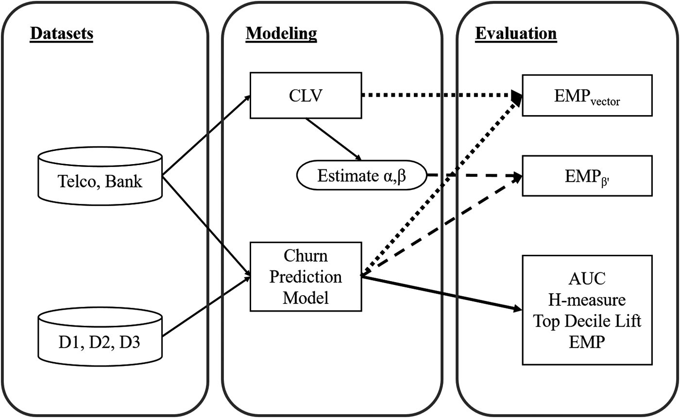
The experimental setup. AUC, area under the ROC curve; CLV, customer lifetime value; EMP, expected maximum profit.

Estimating CLV and distribution parameters

We need the customers' lifetime values to obtain a distribution for the EMP. As the Bank and Telco data sets contain rich enough information to estimate CLV, we proceed using Equations (2) and (3). For the Bank data, we considered the usage of a single product—bank accounts—for a time horizon of 6 months with the aggregated account balance at the end of the month and total amount debited during the same month. In these calculations, we assume that the product yield \documentclass{aastex}\usepackage{amsbsy}\usepackage{amsfonts}\usepackage{amssymb}\usepackage{bm}\usepackage{mathrsfs}\usepackage{pifont}\usepackage{stmaryrd}\usepackage{textcomp}\usepackage{portland, xspace}\usepackage{amsmath, amsxtra}\usepackage{upgreek}\pagestyle{empty}\DeclareMathSizes{10}{9}{7}{6}\begin{document} $${ \pi _1}$$ \end{document} is directly proportional to the transaction volume and set it to 0.1% and the monthly discounting factor to 0.71%, which corresponds to a yearly discount rate of around 10%. This is in line with previous research.⁹

In the case of Telco data sets, the CLV was computed with data from the last 3 months, based on contract information from the telecommunication provider. For postpaid contracts, the monthly subscription fee is €15, and includes unlimited number of text messages and 120 minutes of phone calls. Each additional minute costs €0.15. A decision was made to omit the discounting factor in these calculations because the time period was only 3 months.

The five remaining data sets in Table 3 do not contain enough information to compute CLV. As we know they are from the telecommunication industry, we can still apply our suggested approach if we have knowledge about the distribution of CLV in similar businesses. Four additional CDR data sets, originating from a telecommunication provider in Belgium, were, therefore, used to compute CLV as described for the data set Telco to estimate reference values of parameters \documentclass{aastex}\usepackage{amsbsy}\usepackage{amsfonts}\usepackage{amssymb}\usepackage{bm}\usepackage{mathrsfs}\usepackage{pifont}\usepackage{stmaryrd}\usepackage{textcomp}\usepackage{portland, xspace}\usepackage{amsmath, amsxtra}\usepackage{upgreek}\pagestyle{empty}\DeclareMathSizes{10}{9}{7}{6}\begin{document} $$\alpha$$ \end{document} and \documentclass{aastex}\usepackage{amsbsy}\usepackage{amsfonts}\usepackage{amssymb}\usepackage{bm}\usepackage{mathrsfs}\usepackage{pifont}\usepackage{stmaryrd}\usepackage{textcomp}\usepackage{portland, xspace}\usepackage{amsmath, amsxtra}\usepackage{upgreek}\pagestyle{empty}\DeclareMathSizes{10}{9}{7}{6}\begin{document} $$\beta$$ \end{document} in Equation (4), see Table 4. Two of the data sets spanned 6 months and two spanned 3 months of call traffic between customers.

Table 4.

Parameter estimates of α and β

Data set	α	β
CDR1	1269	2.077
CDR2	158	2.010
CDR3	2817	2.083
CDR4	227	2.012

CDR, call detail record.

The parameter estimates given in Table 4 show that estimates for the \documentclass{aastex}\usepackage{amsbsy}\usepackage{amsfonts}\usepackage{amssymb}\usepackage{bm}\usepackage{mathrsfs}\usepackage{pifont}\usepackage{stmaryrd}\usepackage{textcomp}\usepackage{portland, xspace}\usepackage{amsmath, amsxtra}\usepackage{upgreek}\pagestyle{empty}\DeclareMathSizes{10}{9}{7}{6}\begin{document} $$\beta$$ \end{document} parameter are rather similar, whereas the variation in the \documentclass{aastex}\usepackage{amsbsy}\usepackage{amsfonts}\usepackage{amssymb}\usepackage{bm}\usepackage{mathrsfs}\usepackage{pifont}\usepackage{stmaryrd}\usepackage{textcomp}\usepackage{portland, xspace}\usepackage{amsmath, amsxtra}\usepackage{upgreek}\pagestyle{empty}\DeclareMathSizes{10}{9}{7}{6}\begin{document} $$\alpha$$ \end{document} parameter is greater. This can be explained by the fact that the first and the third CDR are with postpaid contracts, whereas the second and the fourth contain phone usage of customers with prepaid contracts. In general, there is less traffic in the prepaid case, which explains the difference in the estimate for \documentclass{aastex}\usepackage{amsbsy}\usepackage{amsfonts}\usepackage{amssymb}\usepackage{bm}\usepackage{mathrsfs}\usepackage{pifont}\usepackage{stmaryrd}\usepackage{textcomp}\usepackage{portland, xspace}\usepackage{amsmath, amsxtra}\usepackage{upgreek}\pagestyle{empty}\DeclareMathSizes{10}{9}{7}{6}\begin{document} $$\alpha$$ \end{document} . In addition, the first two data sets are from the year 2010 and the second two from the year 2015, which can explain the increase in the \documentclass{aastex}\usepackage{amsbsy}\usepackage{amsfonts}\usepackage{amssymb}\usepackage{bm}\usepackage{mathrsfs}\usepackage{pifont}\usepackage{stmaryrd}\usepackage{textcomp}\usepackage{portland, xspace}\usepackage{amsmath, amsxtra}\usepackage{upgreek}\pagestyle{empty}\DeclareMathSizes{10}{9}{7}{6}\begin{document} $$\alpha$$ \end{document} values.

The parameter estimates can be used as a reference by telecommunication providers that wish to evaluate their churn prediction models using \documentclass{aastex}\usepackage{amsbsy}\usepackage{amsfonts}\usepackage{amssymb}\usepackage{bm}\usepackage{mathrsfs}\usepackage{pifont}\usepackage{stmaryrd}\usepackage{textcomp}\usepackage{portland, xspace}\usepackage{amsmath, amsxtra}\usepackage{upgreek}\pagestyle{empty}\DeclareMathSizes{10}{9}{7}{6}\begin{document} $${\rm {EMP}}_{\beta \prime}$$ \end{document} .

Results when CLV is known

First of all, we look at Figure 2, which demonstrates the value of the regular EMP and EMP fraction as a function of CLV for the data set Telco. What these figures show, especially the first one, is that there is a linear relationship between these two parameters, and, therefore, that using a fixed CLV may give predictable results. This relationship is not as strong for the EMP fraction, but it is noticeable that it converges to 1 when the CLV gets close to 50,000.

FIG. 2.

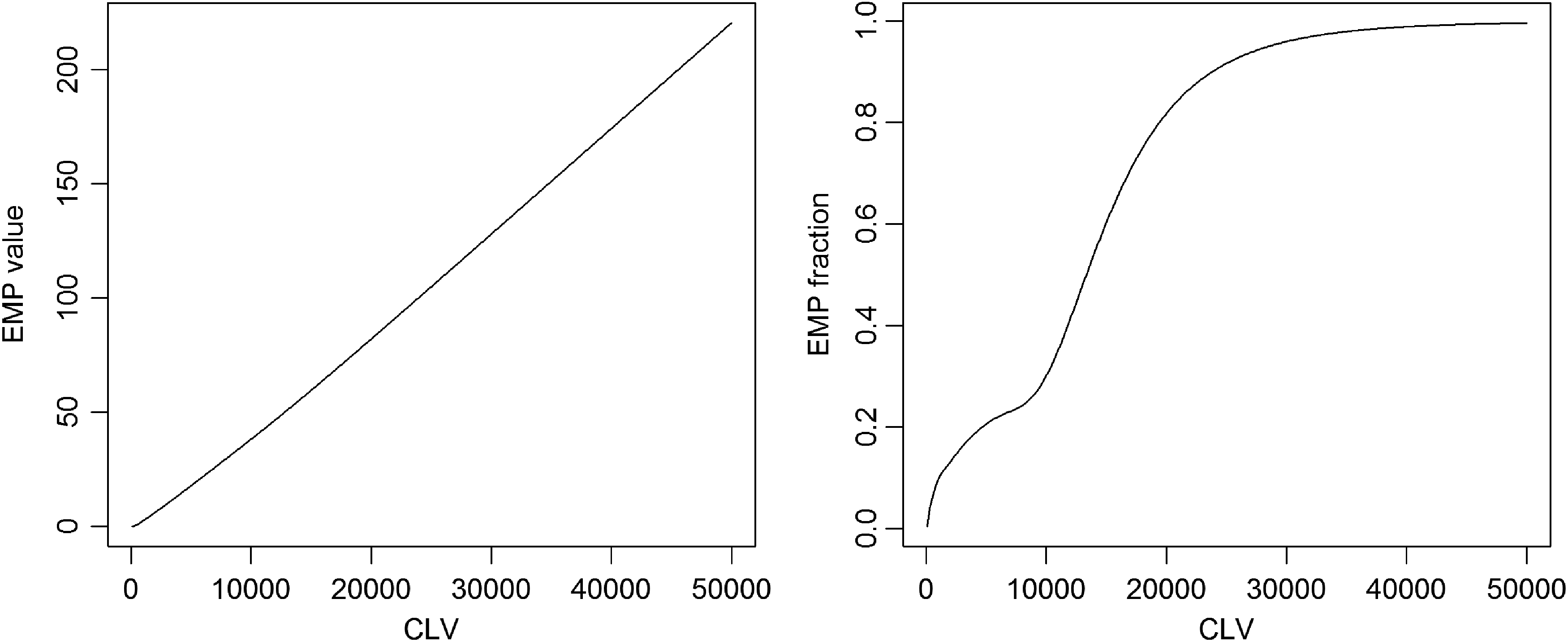
EMP and EMP fraction as functions of CLV.

Next, we look at the comparison of the performance measures for the data sets wherein the CLV is computable, namely the data sets Telco and Bank, see Table 5. The table shows the performance of the three types of models LR, DT, and RF measured in AUC, H-measure, top decile lift, and the regular EMP measure. We used the computed vector of CLV to compute \documentclass{aastex}\usepackage{amsbsy}\usepackage{amsfonts}\usepackage{amssymb}\usepackage{bm}\usepackage{mathrsfs}\usepackage{pifont}\usepackage{stmaryrd}\usepackage{textcomp}\usepackage{portland, xspace}\usepackage{amsmath, amsxtra}\usepackage{upgreek}\pagestyle{empty}\DeclareMathSizes{10}{9}{7}{6}\begin{document} $${{ \rm{EMP}}_{vector}}$$ \end{document} and extracted its mean and median value, as seen in the fifth and sixth columns of Table 5. Subsequently, using the vectors of CLV as representatives of the prior distribution, the method of moments in Equation (4) was used to estimate the parameters \documentclass{aastex}\usepackage{amsbsy}\usepackage{amsfonts}\usepackage{amssymb}\usepackage{bm}\usepackage{mathrsfs}\usepackage{pifont}\usepackage{stmaryrd}\usepackage{textcomp}\usepackage{portland, xspace}\usepackage{amsmath, amsxtra}\usepackage{upgreek}\pagestyle{empty}\DeclareMathSizes{10}{9}{7}{6}\begin{document} $$\alpha$$ \end{document} and \documentclass{aastex}\usepackage{amsbsy}\usepackage{amsfonts}\usepackage{amssymb}\usepackage{bm}\usepackage{mathrsfs}\usepackage{pifont}\usepackage{stmaryrd}\usepackage{textcomp}\usepackage{portland, xspace}\usepackage{amsmath, amsxtra}\usepackage{upgreek}\pagestyle{empty}\DeclareMathSizes{10}{9}{7}{6}\begin{document} $$\beta$$ \end{document} of a \documentclass{aastex}\usepackage{amsbsy}\usepackage{amsfonts}\usepackage{amssymb}\usepackage{bm}\usepackage{mathrsfs}\usepackage{pifont}\usepackage{stmaryrd}\usepackage{textcomp}\usepackage{portland, xspace}\usepackage{amsmath, amsxtra}\usepackage{upgreek}\pagestyle{empty}\DeclareMathSizes{10}{9}{7}{6}\begin{document} $${\beta \prime}$$ \end{document} distribution. The last two columns show the mean and median values of EMP using CLV sampled from the obtained \documentclass{aastex}\usepackage{amsbsy}\usepackage{amsfonts}\usepackage{amssymb}\usepackage{bm}\usepackage{mathrsfs}\usepackage{pifont}\usepackage{stmaryrd}\usepackage{textcomp}\usepackage{portland, xspace}\usepackage{amsmath, amsxtra}\usepackage{upgreek}\pagestyle{empty}\DeclareMathSizes{10}{9}{7}{6}\begin{document} $${\beta \prime}$$ \end{document} distribution.

Table 5.

Comparison of the performance measures

		Measure
Data set	Method	AUC	H-measure	Top decile lift	EMP	Mean EMP _vector	Median EMP _vector	Mean EMP _β′	Median EMP _β′
Telco	LR	0.921	0.583	1.21	0.107	4.86	1.42 · 10⁻⁹	3.53	1.61
α = 2669	DT	0.887	0.554	1.83	0.117	4.65	8.07 · 10⁻⁶	3.40	1.55
β = 2.077	RF	0.943	0.665	1.45	0.175	5.02	4.16 · 10⁻¹²	3.85	1.89
Bank	LR	0.693	0.118	1.04	0	95.49	11.64	96.34	52.98
α = 26103	DT	0.613	0.0947	1.28	1.25 · 10⁻⁷	95.26	10.87	100.93	53.01
β = 2.001	RF	0.719	0.144	1.09	1.24 · 10⁻¹⁰	95.68	12.13	96.56	52.93

AUC, area under the ROC curve; DT, decision tree; EMP, expected maximum profit; LR, logistic regression; RF, random forest.

The various performance measures given in Table 5 do not agree on the best model. For the Telco data set, for example, DT outperforms in terms of top decile lift but performs worst when measured in terms of AUC and H-measure. The LR model scores worst when measured in terms of top decile lift and EMP, but second best according to all other measures. Even the mean and median values of \documentclass{aastex}\usepackage{amsbsy}\usepackage{amsfonts}\usepackage{amssymb}\usepackage{bm}\usepackage{mathrsfs}\usepackage{pifont}\usepackage{stmaryrd}\usepackage{textcomp}\usepackage{portland, xspace}\usepackage{amsmath, amsxtra}\usepackage{upgreek}\pagestyle{empty}\DeclareMathSizes{10}{9}{7}{6}\begin{document} $${{ \rm{EMP}} _{vector}}$$ \end{document} do not agree which model is best: RF is best according to the mean and worst according to the median. In the case of the Bank data set, we see similar behavior. RF is best when measured in terms of AUC and H-measure, but according to top decile lift and EMP, the DT model is again performing best.

Results when CLV is unknown

We already mentioned that in cases when CLV cannot be computed, for example, when the appropriate data are not available, our method can still be applied. We demonstrate this in the case of telecommunication providers using the five additional data sets, D1, D2, D3, D4, and D5 in Table 3. They all originate from the telecommunication industry, and we used the \documentclass{aastex}\usepackage{amsbsy}\usepackage{amsfonts}\usepackage{amssymb}\usepackage{bm}\usepackage{mathrsfs}\usepackage{pifont}\usepackage{stmaryrd}\usepackage{textcomp}\usepackage{portland, xspace}\usepackage{amsmath, amsxtra}\usepackage{upgreek}\pagestyle{empty}\DeclareMathSizes{10}{9}{7}{6}\begin{document} $$\alpha$$ \end{document} and \documentclass{aastex}\usepackage{amsbsy}\usepackage{amsfonts}\usepackage{amssymb}\usepackage{bm}\usepackage{mathrsfs}\usepackage{pifont}\usepackage{stmaryrd}\usepackage{textcomp}\usepackage{portland, xspace}\usepackage{amsmath, amsxtra}\usepackage{upgreek}\pagestyle{empty}\DeclareMathSizes{10}{9}{7}{6}\begin{document} $$\beta$$ \end{document} from the data set Telco to compute their \documentclass{aastex}\usepackage{amsbsy}\usepackage{amsfonts}\usepackage{amssymb}\usepackage{bm}\usepackage{mathrsfs}\usepackage{pifont}\usepackage{stmaryrd}\usepackage{textcomp}\usepackage{portland, xspace}\usepackage{amsmath, amsxtra}\usepackage{upgreek}\pagestyle{empty}\DeclareMathSizes{10}{9}{7}{6}\begin{document} $${ \rm{EMP}}_{ \beta \prime }$$ \end{document} .

The model performance measured in terms of AUC, H-measure, top decile lift, and the standard EMP as well as mean and median of \documentclass{aastex}\usepackage{amsbsy}\usepackage{amsfonts}\usepackage{amssymb}\usepackage{bm}\usepackage{mathrsfs}\usepackage{pifont}\usepackage{stmaryrd}\usepackage{textcomp}\usepackage{portland, xspace}\usepackage{amsmath, amsxtra}\usepackage{upgreek}\pagestyle{empty}\DeclareMathSizes{10}{9}{7}{6}\begin{document} $${ \rm{EMP}}{_{ \beta \prime }}$$ \end{document} can be seen in Table 6. In the table, the highest value for each performance measure within each data set is underlined. In the case of AUC, the values that are not significantly worse than the best one, at the 95% confidence level, based on the test by DeLong et al.,³⁴ are underlined. We see again that not all performance measures agree which model is the best one. Although XGB seems to perform the best overall, the ranking of the methods beyond that is not consistent. Furthermore, the EMP values tend to show very little discrimination, especially for the data sets D1, D2, D3, and D5. The same is true for top decile lift in data sets D1 and D3, where there is very little variation in performance. We see from these results that model selection can be challenging for two reasons. On one hand, the various performance measures may not agree on which model performs best, and on the other hand, since the variation in performance across the same data set may be very low, it is difficult to determine whether the difference in performance is significant enough.

Table 6.

Comparison of measures when EMP_β′ is applied on new data sets

		Measure
Data set	Method	AUC	H-measure	Top decile lift	EMP	Mean EMP _β′	Median EMP _β′
D1	LR	0.75	0.22	1.29	306.63	281.98	172.57
	DT	0.82	0.36	1.47	306.60	288.96	172.22
	RF	0.85	0.41	1.46	306.79	282.77	170.95
	XGB	0.85	0.41	1.51	306.81	283.42	168.68
	NN	0.86	0.44	1.53	306.63	293.89	171.55
	SVM	0.83	0.38	1.51	306.59	297.29	171.58
D2	LR	0.71	0.21	1.86	224.25	213.57	124.91
	DT	0.72	0.26	2.13	224.24	203.94	124.02
	RF	0.75	0.30	2.07	224.26	203.87	124.35
	XGB	0.82	0.38	2.87	224.56	208.62	123.94
	NN	0.73	0.23	1.98	224.13	203.30	123.00
	SVM	0.72	0.23	2.14	224.17	208.99	123.45
D3	LR	0.58	0.03	1.04	389.32	355.01	220.35
	DT	0.62	0.05	1.05	389.32	354.15	220.07
	RF	0.64	0.07	1.05	389.32	365.49	219.67
	XGB	0.64	0.07	1.04	389.32	356.80	218.81
	NN	0.63	0.06	1.03	389.32	365.11	219.39
	SVM	0.58	0.03	1.05	389.32	357.10	218.30
D4	LR	0.69	0.16	1.26	171.54	157.41	92.93
	DT	0.90	0.55	2.86	173.46	158.28	95.06
	RF	0.92	0.58	2.14	174.37	158.78	96.19
	XGB	0.95	0.66	3.39	174.50	159.24	96.10
	NN	0.85	0.43	2.55	173.00	161.57	95.51
	SVM	0.80	0.37	2.02	171.52	165.27	94.60
D5	LR	0.84	0.40	2.29	98.10	90.95	53.03
	DT	0.88	0.64	5.04	97.65	89.66	51.99
	RF	0.91	0.71	3.05	97.90	89.44	52.67
	XGB	0.93	0.75	5.77	98.54	92.41	53.04
	NN	0.75	0.26	2.52	97.54	90.05	51.08
	SVM	0.87	0.48	3.16	97.98	91.89	53.25

The highest value for each performance measure within each data set is underlined. In the case of AUC, the values that are not significantly worse than the best one, at the 95% confidence level, based on the test by DeLong et al.³³ For the other measures, only the highest value is underlined.

NN, artificial neural networks; SVM, support vector machines; XGB, extreme gradient boosting.

We conclude this section by looking at the distribution of the performance values. Figure 3 shows a combination of a boxplot and scatterplot for five of the six performance measures in Table 6. Each boxplot displays the distribution of one performance measure and by connecting the measurements of the same model (dotted lines), we obtain a visualization of the correlation between the performance measures. Based on this figure, we make the following observations. First, the fact that the lines between the AUC and the H-measure hardly cross indicates that they are highly correlated. This confirms earlier research.¹⁸ Next, the lines between AUC, top decile lift, and EMP cross to a great extent, and are thus not correlated. This means that they measure the performance in alternative ways. Finally, there is almost a one-to-one correspondence between the EMP measure and the \documentclass{aastex}\usepackage{amsbsy}\usepackage{amsfonts}\usepackage{amssymb}\usepackage{bm}\usepackage{mathrsfs}\usepackage{pifont}\usepackage{stmaryrd}\usepackage{textcomp}\usepackage{portland, xspace}\usepackage{amsmath, amsxtra}\usepackage{upgreek}\pagestyle{empty}\DeclareMathSizes{10}{9}{7}{6}\begin{document} $${ \rm{EMP}}_{ \beta \prime }$$ \end{document} , which means that they measure the profit of the models consistently. This is expected because both measure the same thing and one is merely an extension of the other. As mentioned before, the added benefit of the \documentclass{aastex}\usepackage{amsbsy}\usepackage{amsfonts}\usepackage{amssymb}\usepackage{bm}\usepackage{mathrsfs}\usepackage{pifont}\usepackage{stmaryrd}\usepackage{textcomp}\usepackage{portland, xspace}\usepackage{amsmath, amsxtra}\usepackage{upgreek}\pagestyle{empty}\DeclareMathSizes{10}{9}{7}{6}\begin{document} $${ \rm{EMP}}_{ \beta \prime }$$ \end{document} measure is that it incorporates the variability of CLV, and thus allows for variance estimates.

FIG. 3.

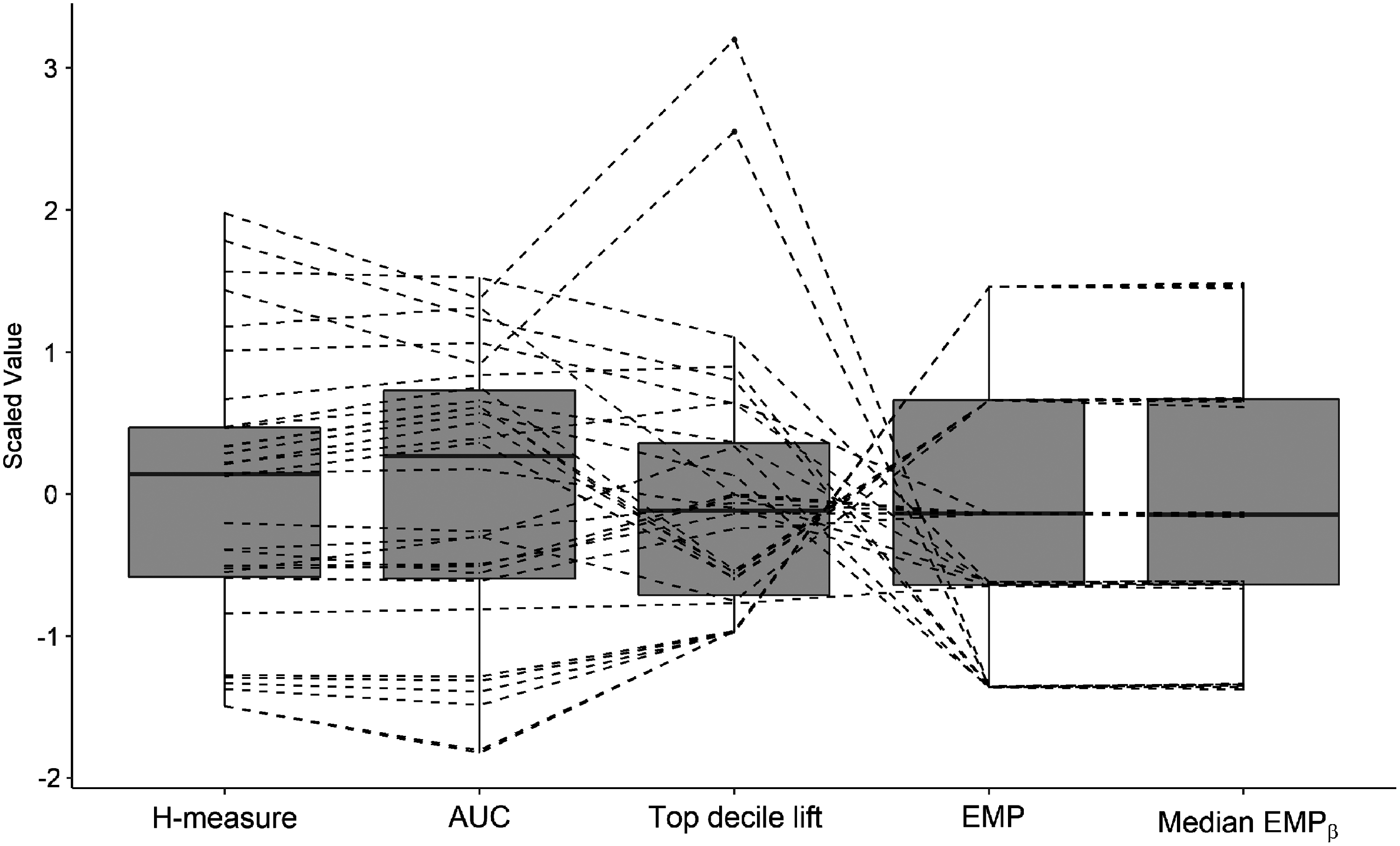
Boxplot and scatterplot showing the correlation among the performance measures.

Managerial Implications

Customer retention is a prevailing problem in many businesses, which makes the design and implementation of campaigns that target the most likely churners an essential part of their operations. From a business perspective, it is furthermore important to not overlook the churners that are most profitable for the business—should they remain. The EMP measure provides a way to assess the profitability of a retention campaign, but with the disadvantage of assuming equal CLVs. To gain deeper insights into customer behavior, our approach shows how the measure can be personalized, thus tailoring the performance measurement to the variability in individual CLVs.

Customer data within organizations have reached unprecedented volumes and keep growing every day. As a result, computing individual CLVs to use in the EMP measure might not be feasible each time a churn prediction model is implemented, since extracting and preparing the data are time consuming and costly. However, as we have demonstrated, the operational costs can be reduced by estimating the parameters of the CLV distribution once and applying the EMP measure with simulated values. Although individual CLVs may be subject to change, the collective CLV distribution typically remains stable for a longer time period. This approach furthermore allows for the computation of confidence intervals for our proposed \documentclass{aastex}\usepackage{amsbsy}\usepackage{amsfonts}\usepackage{amssymb}\usepackage{bm}\usepackage{mathrsfs}\usepackage{pifont}\usepackage{stmaryrd}\usepackage{textcomp}\usepackage{portland, xspace}\usepackage{amsmath, amsxtra}\usepackage{upgreek}\pagestyle{empty}\DeclareMathSizes{10}{9}{7}{6}\begin{document} $${ \rm{EMP}}_{ \beta \prime }$$ \end{document} measure, with the added benefit that the variance in performance can be assessed, thus making it easier to distinguish between the performance of different models.

Table 7 shows 95% confidence intervals for both mean and median of the \documentclass{aastex}\usepackage{amsbsy}\usepackage{amsfonts}\usepackage{amssymb}\usepackage{bm}\usepackage{mathrsfs}\usepackage{pifont}\usepackage{stmaryrd}\usepackage{textcomp}\usepackage{portland, xspace}\usepackage{amsmath, amsxtra}\usepackage{upgreek}\pagestyle{empty}\DeclareMathSizes{10}{9}{7}{6}\begin{document} $${ \rm{EMP}} _{ \beta \prime }$$ \end{document} measures for all seven data sets. This table provides several insights. First of all, by looking at the confidence intervals for the mean and median \documentclass{aastex}\usepackage{amsbsy}\usepackage{amsfonts}\usepackage{amssymb}\usepackage{bm}\usepackage{mathrsfs}\usepackage{pifont}\usepackage{stmaryrd}\usepackage{textcomp}\usepackage{portland, xspace}\usepackage{amsmath, amsxtra}\usepackage{upgreek}\pagestyle{empty}\DeclareMathSizes{10}{9}{7}{6}\begin{document} $${ \rm{EMP}}_{ \beta \prime }$$ \end{document} for the Telco data set, we see that the limits of the RF model do not overlap with the limits of the LR and DT models, and we can conclude that the RF model performs significantly better than the other two models. Next, for the Bank data set, we see that although LR performs badly, the performance is not significantly different from the other two models, so in this case, we can select the simple LR as the best model in terms of profit. Although a RF model may be more powerful, its performance is not necessarily significantly better than a LR model, and, therefore, selecting the model that is simpler and easier to interpret is advantageous for the organization. Our new approach offers the possibility to make that comparison from a profit-driven perspective.

Table 7.

The 95% confidence intervals for EMP_β′

Data set	Method	Mean EMP _β′	Median EMP _β′
Telco	LR	3.53 (3.421–3.630)	1.61 (1.587–1.644)
	DT	3.40 (3.270–3.516)	1.55 (1.530–1.581)
	RF	3.85 (3.724–3.967)	1.89 (1.865–1.924)
Bank	LR	96.34 (93.59–98.88)	52.98 (52.26–53.61)
	DT	100.93 (91.3–107.3)	53.01 (52.27–53.68)
	RF	96.56 (94.32–98.78)	52.93 (52.08–53.65)
D1	LR	281.98 (276.27–287.55)	172.57 (169.93–174.59)
	DT	288.96 (280.84–296.45)	172.22 (170.18–173.94)
	RF	282.77 (275.57–289.21)	170.95 (168.75–173.17)
	XGB	283.42 (275.98–290.11)	168.68 (166.63–170.58)
	NN	293.89 (280–305.22)	171.55 (169.53–173.61)
	SVM	297.29 (281.46–310.24)	171.58 (169.49–173.78)
D2	LR	213.57 (203.37–221.25)	124.91 (123.28–126.53)
	DT	203.94 (199.39–208.28)	124.02 (122.34–125.46)
	RF	203.87 (199.18–208.62)	124.35 (122.93–125.86)
	XGB	208.62 (203.36–213.84)	123.94 (122.48–125.45)
	NN	203.30 (199.18–207.29)	123.00 (121.48–124.61)
	SVM	208.99 (202.61–214.72)	123.45 (121.74–124.9)
D3	LR	355.01 (347.81–361.75)	220.35 (217.88–222.96)
	DT	354.15 (347.07–360.81)	220.07 (217.41–222.89)
	RF	365.49 (356.99–373.65)	219.67 (217.18–222.54)
	XGB	356.80 (349.76–363.84)	218.81 (215.92–221.4)
	NN	365.11 (354.92–374)	219.39 (216.98–222.4)
	SVM	357.10 (350.05–363.9)	218.30 (215.67–220.62)
D4	LR	157.41 (153.71–160.83)	92.93 (91.74–94.14)
	DT	158.28 (155.04–161.39)	95.06 (93.99–96.17)
	RF	158.78 (154.6–162.48)	96.19 (95.08–97.32)
	XGB	159.24 (154.97–163.11)	96.10 (95.03–97.38)
	NN	161.57 (157.39–165.51)	95.51 (94.43–96.69)
	SVM	165.27 (158.62–171.19)	94.60 (93.54–95.8)
D5	LR	90.95 (89.13–92.74)	53.03 (52.26–53.76)
	DT	89.66 (87.63–91.68)	51.99 (51.24–52.72)
	RF	89.44 (87.66–91.19)	52.67 (52–53.26)
	XGB	92.41 (88.93–95.3)	53.04 (52.29–53.68)
	NN	90.05 (87.48–92.57)	51.08 (50.38–51.76)
	SVM	91.89 (89.61–94.04)	53.25 (52.63–53.95)

Furthermore, organizations that do not have the opportunity or the resources to compute lifetime values of their customers can make use of our approach. By relying on parameter estimates from similar businesses, they can achieve estimates for EMP and their corresponding confidence intervals, as we demonstrated for telecommunication companies. Table 7 gives the confidence intervals for the mean and median \documentclass{aastex}\usepackage{amsbsy}\usepackage{amsfonts}\usepackage{amssymb}\usepackage{bm}\usepackage{mathrsfs}\usepackage{pifont}\usepackage{stmaryrd}\usepackage{textcomp}\usepackage{portland, xspace}\usepackage{amsmath, amsxtra}\usepackage{upgreek}\pagestyle{empty}\DeclareMathSizes{10}{9}{7}{6}\begin{document} $${ \rm {EMP}}_{ \beta \prime }$$ \end{document} for data sets D1–D5. In addition, Figure 4 shows a comparison of three performance measures, AUC, top decile lift, and median \documentclass{aastex}\usepackage{amsbsy}\usepackage{amsfonts}\usepackage{amssymb}\usepackage{bm}\usepackage{mathrsfs}\usepackage{pifont}\usepackage{stmaryrd}\usepackage{textcomp}\usepackage{portland, xspace}\usepackage{amsmath, amsxtra}\usepackage{upgreek}\pagestyle{empty}\DeclareMathSizes{10}{9}{7}{6}\begin{document} $${ \rm {EMP}}_{ \beta \prime }$$ \end{document} with confidence intervals, for data set D5. In Figure 4, the black lines portray the \documentclass{aastex}\usepackage{amsbsy}\usepackage{amsfonts}\usepackage{amssymb}\usepackage{bm}\usepackage{mathrsfs}\usepackage{pifont}\usepackage{stmaryrd}\usepackage{textcomp}\usepackage{portland, xspace}\usepackage{amsmath, amsxtra}\usepackage{upgreek}\pagestyle{empty}\DeclareMathSizes{10}{9}{7}{6}\begin{document} $${ \rm {EMP}}_{ \beta \prime }$$ \end{document} performance, with values on the left y-axis, and the stars and triangles show the values of the AUC and top decile lift measures, respectively. On the right y-axis, the upper number corresponds to the AUC value and the lower number corresponds to the top decile lift value. The figure clearly shows that the NN model is significantly worse than the others, a conclusion we could not obtain from Table 6 alone.

FIG. 4.

Confidence intervals for median \documentclass{aastex}\usepackage{amsbsy}\usepackage{amsfonts}\usepackage{amssymb}\usepackage{bm}\usepackage{mathrsfs}\usepackage{pifont}\usepackage{stmaryrd}\usepackage{textcomp}\usepackage{portland, xspace}\usepackage{amsmath, amsxtra}\usepackage{upgreek}\pagestyle{empty}\DeclareMathSizes{10}{9}{7}{6}\begin{document} $${\beta \prime}$$ \end{document} together with model performance measured in AUC (stars) and top decile lift (triangles) for data set D5. DT, decision tree; LR, logistic regression; NN, artificial neural networks; RF, random forest; SVMs, support vector machines; XGB, extreme gradient boosting.

The EMP measure is not only applicable for evaluating churn prediction models. It can be applied to credit risk modeling, time series forecasting, and, consequently, provides increased model interpretability, enhances operational efficiency, and adds value to other businesses as well.

Conclusion

Measuring the performance of CCP models is an important task, especially in organizations that, in addition to being concerned about their own profit, strive to retain their customers in saturated and competitive markets such as telecommunications and banking. In addition, the effectiveness of implementing such models can be increased if the way in which they are measured is tailored toward the problem at hand. This is the case for the EMP measure, which computes the EMP of a retention campaign. This measure of model performance depends on the CLV and it is, therefore, feasible to take into account its naturally occurring variability and heterogeneity when estimating model performance.

We have demonstrated how this can be achieved, both when individual CLVs have been computed and when information about their distribution is available. The results are presented in both cases. When CLV is known, we can compare both mean and median value of the EMP vector to other performance measures, and when the distribution is known, confidence intervals can be extracted to further distinguish actual separation in performance between two models. This extension to the expected maximum profit measure is therefore more informative, as it can be used by practitioners to determine whether there is a significant difference between the performance of two models in terms of EMP. Our proposed extension of measuring the EMP accommodates the data-driven culture that has manifested itself within organizations. It can aid in selecting the best performing model for deployment in retention campaigns. By taking into account the variability in CLV, it focuses on the heterogeneity of customers as is compliant with modern business analytics. Even for on-going customer retention and attrition in fast moving markets, we have demonstrated how the prior knowledge about customers' lifetime values can be used to conveniently measure model performance, in a way that is most beneficial for the company.

We conclude this article with a discussion about its limitations that can be used as a foundation for future research. First, the CLVs were computed in a simple way, since the goal was only to demonstrate how to use them in the EMP measure. In a real-life setting, they should be modeled more carefully. In addition, we have assumed that the CLV follows a \documentclass{aastex}\usepackage{amsbsy}\usepackage{amsfonts}\usepackage{amssymb}\usepackage{bm}\usepackage{mathrsfs}\usepackage{pifont}\usepackage{stmaryrd}\usepackage{textcomp}\usepackage{portland, xspace}\usepackage{amsmath, amsxtra}\usepackage{upgreek}\pagestyle{empty}\DeclareMathSizes{10}{9}{7}{6}\begin{document} $${\beta \prime}$$ \end{document} distribution and estimated the shape parameters accordingly. However, it would be interesting to study other distributions as well, such as Pareto, gamma, negative binomial, or mixtures of distributions. Our experimental evaluation demonstrates only the feasibility of the approach. In a follow-up study with more real-life data sets and multiple classification techniques, using the bootstrap method to compute confidence intervals for the mean and median of \documentclass{aastex}\usepackage{amsbsy}\usepackage{amsfonts}\usepackage{amssymb}\usepackage{bm}\usepackage{mathrsfs}\usepackage{pifont}\usepackage{stmaryrd}\usepackage{textcomp}\usepackage{portland, xspace}\usepackage{amsmath, amsxtra}\usepackage{upgreek}\pagestyle{empty}\DeclareMathSizes{10}{9}{7}{6}\begin{document} $${ \rm{EMP}}_{vector}$$ \end{document} and \documentclass{aastex}\usepackage{amsbsy}\usepackage{amsfonts}\usepackage{amssymb}\usepackage{bm}\usepackage{mathrsfs}\usepackage{pifont}\usepackage{stmaryrd}\usepackage{textcomp}\usepackage{portland, xspace}\usepackage{amsmath, amsxtra}\usepackage{upgreek}\pagestyle{empty}\DeclareMathSizes{10}{9}{7}{6}\begin{document} $${ \rm{EMP}}_{ \beta \prime }$$ \end{document} would allow us to compare these measures with the standard EMP statistically. In addition, there would be opportunity to empirically evaluate the difference in performance of churn prediction models. As a result, it would enable us to generalize these findings, make them more robust, in addition to gaining further insights. We are also not able to address the effectiveness of a particular retention campaign. Finally, as the data sets do unfortunately not contain ground truth about the profit estimates, it is difficult to estimate their accuracy. The addition of such information would be an interesting extension of this research and provide valuable insights to the model selection process.

Footnotes

Acknowledgments

The research was funded by the Flemish Fund for Scientific Research (FWO) and a Belgian bank.

Author Disclosure Statement

No competing financial interests exist.

Cite this article as: Óskarsdóttir M, Baesens B, Vanthienen J (2018) Profit-based model selection for customer retention using individual customer lifetime values. Big Data 6:1, 53–65, DOI: 10.1089/big.2018.0015.

Abbreviations Used

References

Agarwal

, Dhar

. Big data, data science, and analytics: The opportunity and challenge for is research. Inf Syst Res. 2014; 25:443–448.

Brown

, Mues

. An experimental comparison of classification algorithms for imbalanced credit scoring data sets. Expert Syst Appl. 2012; 39:3446–3453.

Verbeke

, Dejaeger

, Martens

, et al. New insights into churn prediction in the telecommunication sector: A profit driven data mining approach. Eur J Oper Res. 2012; 218:211–229.

Rajalakshmi

, Aravindan

. Naive bayes approach for website classification. In: Das

, Thomas

, Gaol

(Eds.): Information Technology and Mobile Communication. Communications in Computer and Information Science, vol 147. Berlin, Heidelberg: Springer, 2011, pp. 323–326.

Verbraken

, Verbeke

, Baesens

. A novel profit maximizing metric for measuring classification performance of customer churn prediction models. IEEE Trans Knowl Data Eng. 2013; 25:961–973.

Verbraken

, Bravo

, Weber

, Baesens

. Development and application of consumer credit scoring models using profit-based classification measures. Eur J Oper Res. 2014; 238:505–513.

Stripling

, vanden Broucke

, Antonio

, et al. Profit maximizing logistic model for customer churn prediction using genetic algorithms. Swarm Evol Comput. 2017. [Epub ahead of print]; DOI: https://doi.org/10.1016/j.swevo.2017.10.010.

Maldonado

, Bravo

, López

, Pérez

. Integrated framework for profit-based feature selection and SVM classification in credit scoring. Decis Support Syst. 2017; 104:113–121.

Glady

, Baesens

, Croux

. Modeling churn using customer lifetime value. Eur J Oper Res. 2009; 197:402–411.

10.

Kumar

. Customer lifetime value—the path to profitability. Found Trends Market. 2008; 2:1–96.

11.

Blattberg

, Malthouse

, Neslin

. Customer lifetime value: Empirical generalizations and some conceptual questions. J Interact Market, 2009; 23:157–168.

12.

Gupta

, Hanssens

, Hardie

, et al. Modeling customer lifetime value. J Service Res. 2006; 9:139–155.

13.

Fader

, Hardie

. Customer-base valuation in a contractual setting: The perils of ignoring heterogeneity. Market Sci. 2010; 29:85–93.

14.

McCarthy

, Fader

, Hardie

. 2016. V(CLV): Examining variance in models of customer lifetime value. Available online at https://ssrn.com/abstract=2739475.

15.

Fawcett

. An introduction to roc analysis. Pattern Recognit Lett. 2006; 27:861–874.

16.

Hand

. Measuring classifier performance: A coherent alternative to the area under the ROC curve. Mach Learn. 2009; 77:103–123.

17.

Ferri

, Hernández-Orallo

, Flach

. A coherent interpretation of auc as a measure of aggregated classification performance. In: Proceedings of the 28th International Conference on Machine Learning (ICML-11), Bellevue, Washington, June 28–July 2, 2011, pp. 657–664.

18.

Lessmann

, Baesens

, Seow

H-V

, Thomas

. Benchmarking state-of-the-art classification algorithms for credit scoring: An update of research. Eur J Oper Res. 2015; 247:124–136.

19.

Neslin

, Gupta

, Kamakura

et al. Defection detection: Measuring and understanding the predictive accuracy of customer churn models. J Mark Res. 2006; 43:204–211.

20.

Davenport

, Harris

, Shapiro

. Competing on talent analytics. Harv Bus Rev. 2010; 88:52–58.

21.

Jain

, Singh

. Customer lifetime value research in marketing: A review and future directions. J Interact Market. 2002; 16:3–4.

22.

Calciu

. Deterministic and stochastic customer lifetime value models. Evaluating the impact of ignored heterogeneity in non-contractual contexts. J Target Meas Anal Market., 2009; 17:257–271.

23.

Fader

, Hardie

. Probability models for customer-base analysis. J Interact Market. 2009; 23:61–69.

24.

Zhang

, Bradlow

, Small

. Predicting customer value using clumpiness: From rfm to RFMC. Market Sci. 2014; 34:195–208.

25.

Jackson

. Build customer relationships that last. Harv Bus Rev. 1985; 11:120–128.

26.

Casella

, Berger

. Statistical inference, vol. 2. Pacific Grove, CA: Duxbury, 2002.

27.

Efron

, Tibshirani

. An introduction to the bootstrap. Boca Raton, FL: CRC Press, 1994.

28.

Lima

, Mues

, Baesens

. Monitoring and backtesting churn models. Expert Syst Appl. 2011; 38:975–982.

29.

Baesens

. Analytics in a big data world: The essential guide to data science and its applications. Hoboken, NJ: John Wiley & Sons, 2014.

30.

Hung

S-Y

, Yen

, Wang

H-Y

. Applying data mining to telecom churn management. Expert Syst Appl. 2006; 31:515–524.

31.

, He

, Xiong

, Brown

. Customer churn analysis for a software-as-a-service company. In: Systems and Information Engineering Design Symposium (SIEDS), Charlottesville, VA: IEEE, 28–28 April, 2017. pp. 106–111.

32.

Pendharkar

. Genetic algorithm based neural network approaches for predicting churn in cellular wireless network services. Expert Syst Appl. 2009; 36:6714–6720.

33.

Maldonado

, Flores

, Verbraken

, et al. Profit-based feature selection using support vector machines—general framework and an application for customer retention. Appl Soft Comput. 2015; 35:740–748.

34.

DeLong

, DeLong

, Clarke-Pearson

. Comparing the areas under two or more correlated receiver operating characteristic curves: A nonparametric approach. Biometrics. 1988; 44:837–845.