Effects of Pacing Properties on Performance in Long-Distance Running

Abstract

This article focuses on the performance of runners in official races. Based on extensive public data from participants of races organized by the Boston Athletic Association, we demonstrate how different pacing profiles can affect the performance in a race. An athlete's pacing profile refers to the running speed at various stages of the race. We aim to provide practical, data-driven advice for professional as well as recreational runners. Our data collection covers 3 years of data made public by the race organizers, and primarily concerns the times at various intermediate points, giving an indication of the speed profile of the individual runner. We consider the 10 km, half marathon, and full marathon, leading to a data set of 120,472 race results. Although these data were not primarily recorded for scientific analysis, we demonstrate that valuable information can be gleaned from these substantial data about the right way to approach a running challenge. In this article, we focus on the role of race distance, gender, age, and the pacing profile. Since age is a crucial but complex determinant of performance, we first model the age effect in a gender- and distance-specific manner. We consider polynomials of high degree and use cross-validation to select models that are both accurate and of sufficient generalizability. After that, we perform clustering of the race profiles to identify the dominant pacing profiles that runners select. Finally, after having compensated for age influences, we apply a descriptive pattern mining approach to select reliable and informative aspects of pacing that most determine an optimal performance. The mining paradigm produces relatively simple and readable patterns, such that both professionals and amateurs can use the results to their benefit.

Introduction

Running is among the most practiced sports in the world. For practical reasons, it is hard to keep track of all runners in the world and thereby exactly quantify the total number of runners worldwide. However, for certain parts of the world, there are some rough estimations available. According to a survey¹ of Asics, there were around 80 million European runners in 2009, and in 2016, only in the United States already more than 64 million people went jogging or running.² This number includes both the people who train on a regular basis throughout the year and the more occasional runner. Also, participating in a road race is popular. In 2016, there were in total roughly 17 million people who finished a running event in the United States.²

The big technological improvements in the last decades gave runners many new opportunities. In the early days, it was very hard to keep track of information of trainings and race results, whereas nowadays a sports watch or running application is part of the standard equipment of most runners. Therefore, runners now gather data on a lot of athletic aspects, such as distance, pacing, and cadence. For recreational runners, this opened up the possibility to follow a more detailed training schedule. Moreover, it also leads to a growing interest in the information that can be extracted from the data, as it can give an athlete valuable information about how to improve his or her performance in a race.

To perform in a long-distance run, multiple factors are important, such as physically preparing for a race and knowing how to follow a specific pacing strategy. Although data can be used to help improve an athlete's fitness, the age of an athlete limits the physiological basis of endurance. Despite the fact that some of the details are still up for debate, there is general consensus that until a certain age, performance increases and eventually as one gets older, performance decreases, such that there must be an age-related optimum for physiological functional capacity.^3–6 For running, it seems that the optimal age is positively correlated with distance: the longer the distance, the older the optimal age.⁷ This may be further substantiated by the findings of Wiswell et al.⁸ for shorter distances (5 and 10 km).

Apart from optimizing the fitness of an athlete, one of the most important factors for a successful long-distance run is the followed pacing strategy.^9–11 The strategies can be divided into several different categories.¹² The most common pacing strategies are positive pacing (the athlete slows down during the race), negative pacing (the athlete accelerates during the race), and even pacing (constant pace during the race).

Many studies on pacing strategies focus on professional athletes. Although there is no conclusive evidence for an optimal strategy, most analyses find that professional runners perform better when they run at a constant pace or follow a negative pacing strategy.^13,14 Since there are big differences between professional athletes and recreational runners, these findings do not automatically transfer to the amateur runner. For recreational runners, it is found that older runners typically follow a more constant pace than younger athletes who finish in a similar time.¹⁵ Also, by dividing athletes into different groups according to their final time, it is found that faster runners have a smaller variability in their race speed.¹⁶ In addition to pacing variability, there are many other pacing characteristics that could distinguish slower from faster runners, such as minimum or maximum speed, difference between minimum and maximum speed, or simply, say, the relative pace from 5 to 10 km.

Up to now, the main pacing property that differentiates faster from slower runners is still unknown. To find this characteristic, we divide the athletes into two different groups: the fast finishers and the underperformers. To make this distinction, we use age-performance models as a baseline for the physical capacities. If an athlete's final time is shorter than what the age-performance model predicts for his or her age, the runner is a fast finisher. On the contrary, underperformers are athletes who are slower than predicted by the age-performance model.

In this work, we use a data-driven approach to investigate the effect of age, gender, and pacing properties on the performance in long-distance running. We consider the 10 km, half marathon, and full marathon organized by the Boston Athletics Association between 2015 and 2017. In these 3 years, a total of 120,472 race results were recorded, and for each result, we have at our disposal information on age, gender, distance, as well as the sequence of intermediate times that the runner clocked. First, we focus on age effects and develop gender-specific models for the 10 km, half marathon, and full marathon. Subsequently, we determine on each distance the most common pacing profiles, and we look at the relationship between the performance and the pacing profile. Finally, we consider many pacing properties together and use Subgroup Discovery to find the main characteristics that distinguish the fast finishers from the underperformers.

Materials

In this section, we discuss data collection and explain how we transform data into valuable characteristics for the analysis.

Data

In this research, we have used data from the races over 10 km, half marathon, and full marathon, organized by the Boston Athletic Association from 2015 to 2017. These data are accessible online¹⁷ and we have received permission to use this data collection for scientific purposes. For the 10 km race, we have a total of 9596 male and 12,313 female participants. The collection with the results of the half marathon consists of 8586 male and 10,339 female participants. And finally, for the full marathon there are 43,482 male and 36,156 female participants. For each distance, we have the athlete's age in years and the final time of every participant.

For the analysis, we have to account for the fact that some of the variances in results are due to external factors. It is, for example, well known that the weather conditions have strong effects on the performance in long-distance running.^18–20 Moreover, a change in the course can affect the height profile and thereby also influence the recorded final times. Therefore, in our analysis, we work with the relative time.

Definition 1. For an athlete of gender g, the relative time \documentclass{aastex}\usepackage{amsbsy}\usepackage{amsfonts}\usepackage{amssymb}\usepackage{bm}\usepackage{mathrsfs}\usepackage{pifont}\usepackage{stmaryrd}\usepackage{textcomp}\usepackage{portland, xspace}\usepackage{amsmath, amsxtra}\usepackage{upgreek}\pagestyle{empty}\DeclareMathSizes{10}{9}{7}{6}\begin{document} $${t_{{ \rm{rel}}}}$$ \end{document} of a race in the year y with distance d is defined as follows: \documentclass{aastex}\usepackage{amsbsy}\usepackage{amsfonts}\usepackage{amssymb}\usepackage{bm}\usepackage{mathrsfs}\usepackage{pifont}\usepackage{stmaryrd}\usepackage{textcomp}\usepackage{portland, xspace}\usepackage{amsmath, amsxtra}\usepackage{upgreek}\pagestyle{empty}\DeclareMathSizes{10}{9}{7}{6}\begin{document} \begin{align*} {t_{{ \rm{rel}}}} = t / {t_{{ \rm{med}}}} \left( {d , g , y} \right) , \end{align*} \end{document}

For our data collection, we find that the variability between different years in the relative time is smaller than the variability in recorded final times. Hence, the relative time is a better measure for comparing results between different years.

The relative time is below or above 1 when the final time is faster or slower than the median of the collection of relevant final times, respectively. We have chosen the median over other measures, such as the mean, since it is less sensitive to outliers. In principle, this definition could be used for analyzing the performances on all distances for both genders together, and finding results that are independent of gender and race distance. However, the nature of the distances is quite diverse and the physiological differences between male and female athletes can be important. Therefore, we consider every distance and also men and women separately.

In addition to the final times, we also have 2 intermediate times at 5 and 8 km in the 10 km race and for the participants of the half marathon, we have the 8 and 16 km intermediate times. The data of the full marathon are richer and contain intermediate times after every 5 km and halfway the full marathon.

There are participants for whom (some of) the intermediate times are missing or the intermediate time measurements are incorrect. We were able to check the quality of the data using some known limits. For example, we could exclude any measurements where the time on a certain interval was negative. Slightly more detailed, we also excluded some data points based on a maximum feasible speed between successive intermediate points by using the distance-specific world records. Roughly, we take a 10% margin to allow athletes to run slightly faster than the average world record pace on a particular interval. Thus for men, we set speed limits of 25, 24, and 23 km/h for the 10 km, half marathon, and full marathon, respectively. For women, we use limits of 23, 22, and 21 km/h for the three distances. By removing these participants from the data collection, we are left with 9464 runners in the 10 km events, 8480 athletes in the half marathon races, and 43,125 male participants for the full marathon. Thus, for the three distances, only 1.4%, 1.2%, and 0.8% of the male runners have intermediate times that are incomplete or incorrect. The number of female participants who satisfy the speed limit criteria are 12,189 for the 10 km, 10,205 for the half marathon races, and 35,906 for the full marathon. Thus, for women, 1.0%, 1.3%, and 0.7% of the participants are excluded for the 10 km, half marathon, and full marathon, respectively.

For each distance, there are differences in the distance between two successive intermediate points. Therefore, instead of taking the time difference between two adjacent intermediate times, we consider the average speed between the two successive intermediate points. Moreover, absolute speeds do not allow for a fair comparison of pace variations in a race between athletes who run at different average speeds. Therefore, we introduce the relative pace.

Definition 2. The relative pace \documentclass{aastex}\usepackage{amsbsy}\usepackage{amsfonts}\usepackage{amssymb}\usepackage{bm}\usepackage{mathrsfs}\usepackage{pifont}\usepackage{stmaryrd}\usepackage{textcomp}\usepackage{portland, xspace}\usepackage{amsmath, amsxtra}\usepackage{upgreek}\pagestyle{empty}\DeclareMathSizes{10}{9}{7}{6}\begin{document} $${p_{{ \rm{rel}}}}$$ \end{document} between two intermediate points \documentclass{aastex}\usepackage{amsbsy}\usepackage{amsfonts}\usepackage{amssymb}\usepackage{bm}\usepackage{mathrsfs}\usepackage{pifont}\usepackage{stmaryrd}\usepackage{textcomp}\usepackage{portland, xspace}\usepackage{amsmath, amsxtra}\usepackage{upgreek}\pagestyle{empty}\DeclareMathSizes{10}{9}{7}{6}\begin{document} $${x_{ \rm{a}}}$$ \end{document} and \documentclass{aastex}\usepackage{amsbsy}\usepackage{amsfonts}\usepackage{amssymb}\usepackage{bm}\usepackage{mathrsfs}\usepackage{pifont}\usepackage{stmaryrd}\usepackage{textcomp}\usepackage{portland, xspace}\usepackage{amsmath, amsxtra}\usepackage{upgreek}\pagestyle{empty}\DeclareMathSizes{10}{9}{7}{6}\begin{document} $${x_{ \rm{b}}}$$ \end{document} is defined as follows: \documentclass{aastex}\usepackage{amsbsy}\usepackage{amsfonts}\usepackage{amssymb}\usepackage{bm}\usepackage{mathrsfs}\usepackage{pifont}\usepackage{stmaryrd}\usepackage{textcomp}\usepackage{portland, xspace}\usepackage{amsmath, amsxtra}\usepackage{upgreek}\pagestyle{empty}\DeclareMathSizes{10}{9}{7}{6}\begin{document} \begin{align*} {p_{{ \rm{rel}}}} \left( {{x_{ \rm{a}}} , {x_{ \rm{b}}}} \right) = v \left( {{x_{ \rm{a}}} , {x_{ \rm{b}}}} \right) / {v_{{ \rm{avg}}}} , \end{align*} \end{document}

where \documentclass{aastex}\usepackage{amsbsy}\usepackage{amsfonts}\usepackage{amssymb}\usepackage{bm}\usepackage{mathrsfs}\usepackage{pifont}\usepackage{stmaryrd}\usepackage{textcomp}\usepackage{portland, xspace}\usepackage{amsmath, amsxtra}\usepackage{upgreek}\pagestyle{empty}\DeclareMathSizes{10}{9}{7}{6}\begin{document} $$v \left( {{x_{ \rm{a}}} , {x_{ \rm{b}}}} \right)$$ \end{document} is the average speed between two intermediate points \documentclass{aastex}\usepackage{amsbsy}\usepackage{amsfonts}\usepackage{amssymb}\usepackage{bm}\usepackage{mathrsfs}\usepackage{pifont}\usepackage{stmaryrd}\usepackage{textcomp}\usepackage{portland, xspace}\usepackage{amsmath, amsxtra}\usepackage{upgreek}\pagestyle{empty}\DeclareMathSizes{10}{9}{7}{6}\begin{document} $${x_{ \rm{a}}}$$ \end{document} and \documentclass{aastex}\usepackage{amsbsy}\usepackage{amsfonts}\usepackage{amssymb}\usepackage{bm}\usepackage{mathrsfs}\usepackage{pifont}\usepackage{stmaryrd}\usepackage{textcomp}\usepackage{portland, xspace}\usepackage{amsmath, amsxtra}\usepackage{upgreek}\pagestyle{empty}\DeclareMathSizes{10}{9}{7}{6}\begin{document} $${x_{ \rm{b}}}$$ \end{document} and \documentclass{aastex}\usepackage{amsbsy}\usepackage{amsfonts}\usepackage{amssymb}\usepackage{bm}\usepackage{mathrsfs}\usepackage{pifont}\usepackage{stmaryrd}\usepackage{textcomp}\usepackage{portland, xspace}\usepackage{amsmath, amsxtra}\usepackage{upgreek}\pagestyle{empty}\DeclareMathSizes{10}{9}{7}{6}\begin{document} $${v_{{ \rm{avg}}}}$$ \end{document} is the average speed during the race.

If the average speed of an athlete between two intermediate points is smaller than 1, the runner is slower than his or her average pace during the entire race. The relative pace is larger than 1 if the athlete is faster than the average speed in the entire race. This definition is especially useful in our analysis, since the relative pace is a proper measure for comparing pacing profiles of athletes who run at a different average speed.

Note that in the data collection there are athletes who participated in multiple races. Therefore, in the collected data, we would obtain results that are slightly biased toward these athletes if we consider all entries together. There are multiple options to circumvent this issue. Participants who ran a particular distance more than once may have altered their pacing based on their previous experience. To compare a runner who runs the marathon for the first time with an athlete who is more experienced is arguably unfair. Therefore, we only consider a runner's first result on a particular distance that falls within the previously mentioned speed limits. Although it still might be that runners from the 2015 marathon ran the marathon in previous years, we consider this the solution with the least known bias. Therefore, we are left with 7793 male and 10,493 female participants for the 10 km. For the half marathon, we have 7292 male and 9078 female participants and there are 36,107 male and 30,884 female participants for the full marathon.

Feature construction

To investigate the pacing properties that can affect the performance in a race, we engineer meaningful features from the raw data. In this section, we discuss the different features that are constructed.

Paces

As discussed in the previous section, the data consist of age, the final time, and a collection of intermediate times for every participant. The first class of features constructed is the relative paces on the different intervals. Instead of considering the relative pace on all possible intervals, we restrict ourselves to the ones that are connected to each other. Hence, in the full marathon, we consider, for example, the relative pace on the intervals 0–5 and 10–30 km, but an interval that consists of the 0–5 and 15–20 km intervals is not considered. For the two shortest distances, there are two intermediate times, and therefore, this approach only gives five features. However, for the full marathon, there are nine intermediate time points and since \documentclass{aastex}\usepackage{amsbsy}\usepackage{amsfonts}\usepackage{amssymb}\usepackage{bm}\usepackage{mathrsfs}\usepackage{pifont}\usepackage{stmaryrd}\usepackage{textcomp}\usepackage{portland, xspace}\usepackage{amsmath, amsxtra}\usepackage{upgreek}\pagestyle{empty}\DeclareMathSizes{10}{9}{7}{6}\begin{document} \begin{align*} \mathop \sum \limits_ { i = 2 } ^ { 10 } { i = \frac { { 10 \cdot ( 10 + 1 ) } } { 2 } } - 1 = 54 , \end{align*} \end{document}

we have 54 features for the relative paces.

We are also interested in measures that quantify the distribution of the relative paces. Therefore, for every athlete, we collect the relative paces between two successive intermediate points. Of this collection, we then consider the following measures of distribution of relative paces²¹: 1.

Minimum

Maximum

Difference between maximum and minimum

Median

Standard deviation

First quartile

Third quartile

Interquartile range

Skewness

10.

Kurtosis

In principle, also other properties can be considered, but we believe that these quantities capture the most valuable information of the distribution of relative paces. Since for the two shortest distances, the collection only consists of three relative paces, we restrict ourselves in this case to the first five elements of this list. In the full marathon, we consider all measures that are listed above. Moreover, in this case, we have 10 different relative paces and we define the first and third quartile as the third smallest or largest relative pace, respectively.

Pace changes

Apart from looking at the relative paces on the different intervals, we also consider the changes in pace during the race. In this study, we define the pace change as the relative drop in speed from one interval to another. Again, we only consider all connected intervals. For the 10 km and half marathon, this implies that we have four different pace changes. The data of the full marathon are richer. Since we have nine intermediate points, and \documentclass{aastex}\usepackage{amsbsy}\usepackage{amsfonts}\usepackage{amssymb}\usepackage{bm}\usepackage{mathrsfs}\usepackage{pifont}\usepackage{stmaryrd}\usepackage{textcomp}\usepackage{portland, xspace}\usepackage{amsmath, amsxtra}\usepackage{upgreek}\pagestyle{empty}\DeclareMathSizes{10}{9}{7}{6}\begin{document} \begin{align*} \mathop \sum \limits_ { i = 1 } ^9 { i \cdot ( 10 - i ) = } 10 \frac { { 9 \cdot \left( { 9 + 1 } \right) } } { 2 } - \left( { \frac { { { 9^3 } } } { 3 } + \frac { { { 9^2 } } } { 2 } + \frac { 9 } { 6 } } \right) = 165 , \end{align*} \end{document}

we have in total 165 features for pace changes. As with the pacing, we also consider different measures of distribution of pace changes. For the full marathon, we consider the same measures as listed before, but for the two shortest distances, we only have a distribution of two pace changes, and therefore, we only consider the first three elements of the list.

Pacing profiles

As mentioned in the Introduction section, the followed pacing strategy is believed to have an impact on performance. Although the previous features already capture some information about pacing, we want to make this more explicit. Therefore, we perform k-Means clustering based on the relative paces between the intermediate points. In this way, we divide all participants into different groups that follow a similar pacing.

First, we have to find a proper value for the number of clusters for men and women on the different distances. In our case, it turns out to be difficult to find an optimal value for this number due to the large variation among runners. This can be seen in Figure 1, where we display the relative sum of squared errors (SSE) as a function of the number of clusters. Ideally, such a graph has a sharp angle that determines the optimal value for the number of clusters.²² For our data collection, the behavior is rather continuous, and therefore, it is not possible to unambiguously identify this so-called elbow point.

FIG. 1.

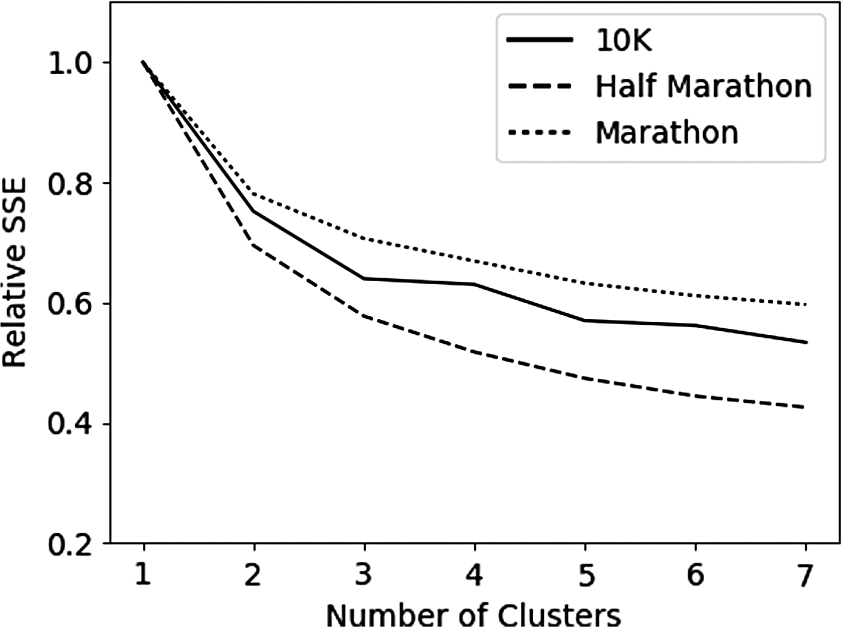
The relative SSE as a function of the number of clusters for men on the three different distances. For every cluster, we calculate the distances between the pacing of an athlete and the centroid of the cluster to which it belongs. The relative SSE is defined as the sum of all these values and to facilitate comparison, we normalized this value with respect to the value of the SSE assuming only a single centroid over the entire data. SSE, sum of squared errors.

In this research, we have opted for a consistent number of clusters among all distances. At some point, adding another cluster will not identify a substantially different pacing profile, or a profile that consists of only a small fraction of athletes. Therefore, we have decided to take three different clusters for both men and women on all three distances. For all athletes, we then determine the distance between their paces and the values for the pace of the centroid of clusters. Therefore, for every athlete, we construct three additional features that capture the distance between pacing and the three most characteristic pacing profiles.

Methods

In our multistep approach, we perform two different types of analysis. First, we perform regression to model the dependence between performance and age of an athlete. In the second part, we use Subgroup Discovery^23–26 to find informative characteristics of fast finishers and underperformers. In this section, we discuss both methods separately.

Regression

As mentioned in the Introduction section, the relationship between age and performance is parabolically shaped. However, the exact details of this relationship can be rather complicated. Therefore, to obtain the model that is the best description of this dependence, it is beneficial to also consider more complicated models than a quadratic function.

In this research, we start with the assumption that the relationship between the output variable, that is, running time, and the regressors, that is, age, can be described by an analytic function. For all practical purposes, this is a valid assumption, since this implies that the function itself and all its derivatives are smooth. Moreover, analytic functions can be represented by a Taylor series. Assuming regression with only a single regressor (in our case, age), we can represent the output variable by the following Taylor polynomial: \documentclass{aastex}\usepackage{amsbsy}\usepackage{amsfonts}\usepackage{amssymb}\usepackage{bm}\usepackage{mathrsfs}\usepackage{pifont}\usepackage{stmaryrd}\usepackage{textcomp}\usepackage{portland, xspace}\usepackage{amsmath, amsxtra}\usepackage{upgreek}\pagestyle{empty}\DeclareMathSizes{10}{9}{7}{6}\begin{document} \begin{align*} y = \mathop \sum \limits_{i = 0}^k { \rm{ }}{a_i}{x^i} , \end{align*} \end{document}

where y is the output variable, x the independent variable, a_i are coefficients, and k is the degree of the polynomial. The regression task is therefore finding the degree k and the corresponding values for the coefficients that give the best estimate for the relationship between x and the dependent variable y. However, we still need to consider the risk of overfitting. Namely, an exact relationship between the output variable and the regressor can be obtained if the number of coefficients is equal to the number of datapoints. However, in this case, the obtained model is too specific to this sample of data and would not generalize to future data.

A common approach to obtain a model that can be generalized to an independent data set is using cross-validation.²⁷ In this research, we use 10-fold cross-validation and perform the following steps. For a choice of k,

Split the data set into 10 distinct parts so that each has a similar distribution for the independent variable. We apply stratified sampling by sorting the data based on the value of the regressor and randomly distributing all 10 successive datapoints over 10 different sets.

Train the model on 90% of the complete data set and obtain values for the k coefficients by using least squares regression.

Calculate the mean squared error (MSE) of the model on the remaining 10% of the data.

Repeat the 2 previous steps in a total 10 times such that each of the 10 sets is used as a validation set once. Add all 10 values of the MSE to obtain the total MSE for the model with a polynomial of degree k.

For small degrees of the polynomial, the sum of the squares of the errors will decrease if the degree of the polynomial increases. Namely, adding new coefficients leads to a model that is a better fit to the data. However, after a certain point, increasing the degree gives a larger total MSE. If the degree is too large, the model is too specific for the training set, and therefore, it will give a large error when validating the model on the remaining 10% of data. Hence, there is a certain degree that has the minimal value for the sum of squares of errors on the validation set and this is the degree of the polynomial that we select for our model. Finally, the value of the corresponding coefficients is then obtained by using ordinary least squares regression on the complete data set.

Subgroup Discovery

In data mining, the goal is finding patterns in the data. It is also interesting to find specific subsets of the data that are characterized by properties that are different than in the entire data collection. A method for finding these subsets is Subgroup Discovery.

To explain Subgroup Discovery, we consider a tabular data set, where the columns represent the variables, or in SD-terminology attributes. As Subgroup Discovery is a so-called supervised technique, every row in the table also contains information about a specified target variable. The target variable t can be either binary, where t can have two different values, or numeric where it can take any value. The goal in Subgroup Discovery is to find a collection of rows, that is, a subgroup of the entire data set, for which the distribution of this target variable is significantly different from the distribution of t in the entire data collection. The interesting part is then to look into the description of the subgroup, which basically restricts the values of one or multiple attributes.

There are two important technical aspects when using Subgroup Discovery. First, it is important to specify a so-called quality measure that determines when exactly the distribution of the target variable in a subgroup is surprisingly different. Quality measures typically take into account the unusualness of the distribution of the target variable and also the size of the subgroup. Depending on the quality measure at hand, there is more emphasis on either of the two aspects. The literature offers many suggestions for quality measures for both numeric and binary target variables.^28–30 Most of the quality measures that are described in these surveys are included in the Cortana Subgroup Discovery tool,³¹ which is the tool used in this project.

The second important part of Subgroup Discovery is to specify the search strategy for finding the interesting subgroups. If the data set is too large, it is namely no longer possible to investigate all possible subgroups in a reasonable time span and we have to use a heuristic technique. For the experiments in this research, we use beam search. In this method, we start from the simple subgroups that are described by a single condition. The quality of each of the subgroups is then evaluated by using the quality measure. We only keep the promising subgroups in the beam, that is, the subgroup with a value for the quality measure that is a higher than a certain default value, and subsequently, the search is extended by adding new conditions to these subgroups. Then, we again calculate the quality of these subgroups and only keep the high-quality subsets. This procedure is repeated until a certain depth \documentclass{aastex}\usepackage{amsbsy}\usepackage{amsfonts}\usepackage{amssymb}\usepackage{bm}\usepackage{mathrsfs}\usepackage{pifont}\usepackage{stmaryrd}\usepackage{textcomp}\usepackage{portland, xspace}\usepackage{amsmath, amsxtra}\usepackage{upgreek}\pagestyle{empty}\DeclareMathSizes{10}{9}{7}{6}\begin{document} $${d_{{ \rm{max}}}}$$ \end{document} is reached, where \documentclass{aastex}\usepackage{amsbsy}\usepackage{amsfonts}\usepackage{amssymb}\usepackage{bm}\usepackage{mathrsfs}\usepackage{pifont}\usepackage{stmaryrd}\usepackage{textcomp}\usepackage{portland, xspace}\usepackage{amsmath, amsxtra}\usepackage{upgreek}\pagestyle{empty}\DeclareMathSizes{10}{9}{7}{6}\begin{document} $${d_{{ \rm{max}}}}$$ \end{document} is equal to the maximum number of restrictions that can be set on the values of the attributes. After a certain point, when we increase the number of conditions, the quality of the obtained subgroups will barely increase. Hence, it is usually sufficient to take a small value for the search depth. In our experiments, this is already the case for small values of d and we limited the search depth to \documentclass{aastex}\usepackage{amsbsy}\usepackage{amsfonts}\usepackage{amssymb}\usepackage{bm}\usepackage{mathrsfs}\usepackage{pifont}\usepackage{stmaryrd}\usepackage{textcomp}\usepackage{portland, xspace}\usepackage{amsmath, amsxtra}\usepackage{upgreek}\pagestyle{empty}\DeclareMathSizes{10}{9}{7}{6}\begin{document} $$d = 2$$ \end{document} .

In addition to setting a value for the depth of the search, we also have to specify the beam width w. The beam width determines the number of subgroups stored during the search. If the value of w is very small, only very few subgroups are extended if the depth of search is increased by one. For very large widths, many more subgroups are stored at the cost of increasing the computational time. For an infinite width, even the entire space of possible subgroups is considered. Therefore, there is a balance between computational time and extensiveness of the search. In the experiments, we specify the value of this parameter.

Results

In this section, we discuss the experimental results. First, we focus on the regression task of modeling the dependence between age and performance.

Age-performance dependence

As explained in the Methods section, the first task is to find the degree of the polynomial. The typical profile for the MSE as a function of the degree of the polynomial of the model is shown in Figure 2. In this figure, we observe that the MSE is parabolically shaped with a large range where the MSE barely changes.

FIG. 2.

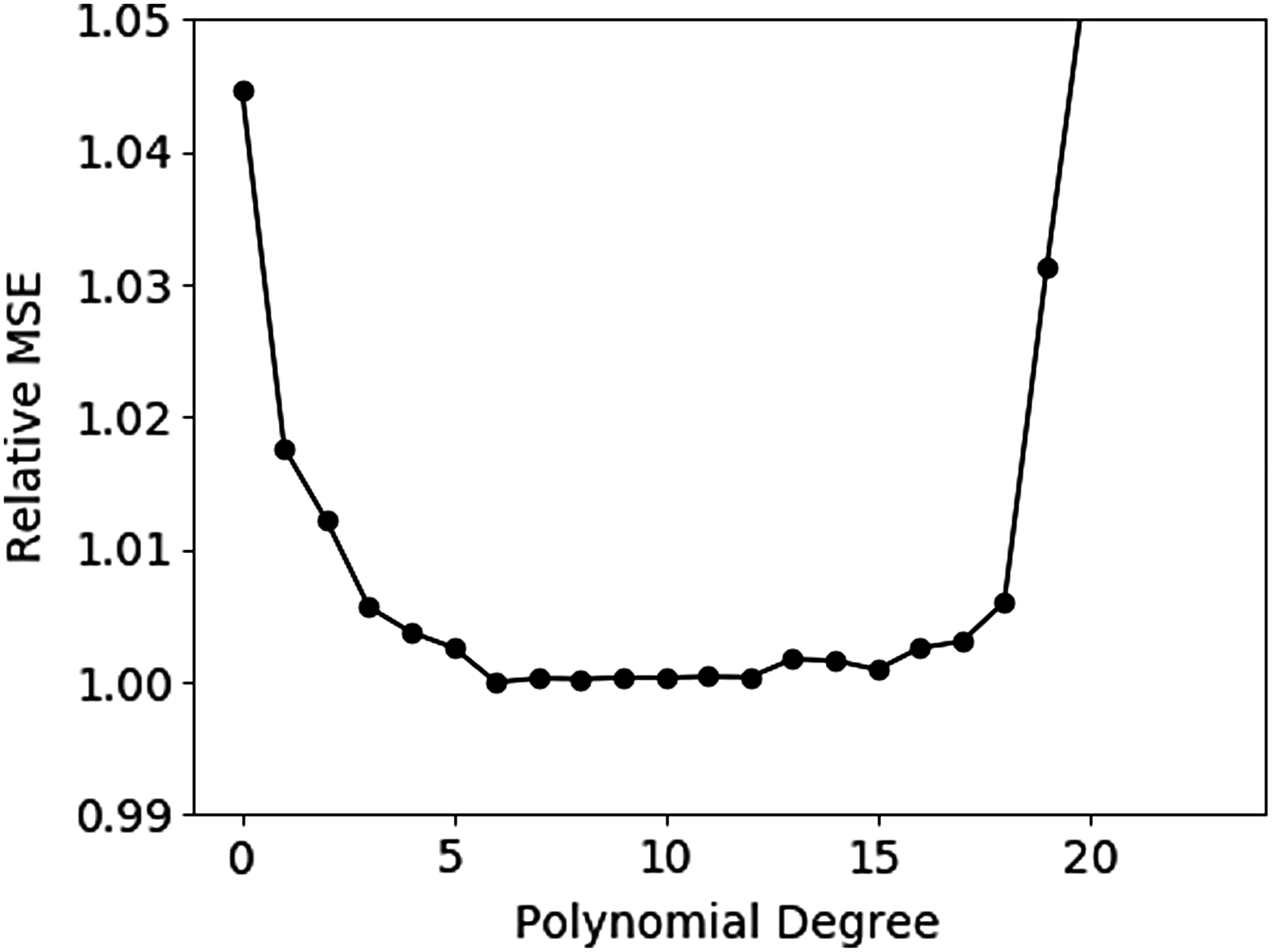
Typical behavior of the relative MSE for different values of the degree of the polynomial. The relative MSE is obtained by normalizing the values with the minimum value of the MSE and this example corresponds to the results of the 10 km races of men. We observe that the MSE first decreases until there is a large plateau where the MSE barely changes. For high polynomial degrees, the MSE rapidly increases. In this case the minimum score is achieved for a polynomial of degree 6. The starting and endpoints of this plateau depend on the distance and whether we consider male or female athletes. MSE, mean squared error.

Since the differences between the MSE of the models inside this range are so small, the polynomial degree with the minimal MSE depends on the division of data over 10 different sets. As this is partly a random process, we performed the procedure explained in the Methods section 1000 times and selected the degree that occurs most often as the one with the minimal MSE. To specify the accuracy of the models, we also determined the 95% confidence intervals. We calculated these intervals by using a bootstrap method by resampling residuals.³² Thus, we determined all residuals and then randomly added a residual to the relative time of every athlete without changing the age of the runners. Then, we used these new data to fit the model with the same polynomial degree. We repeated the complete procedure 1000 times. Hence, for every age within the domain, we have 1000 different predicted values for the relative time. The upper (lower) boundary of the 95% confidence interval is then obtained by taking the 25th smallest (largest) value.

In Table 1, we display the three degrees with highest occurrence after performing a thousand runs. We see from this table that the number of experiments is large enough to find a unique value for the polynomial degree of the model, by simply selecting the degree that occurs most often in the experiments. In this table, we observe that in most cases the degree of the models is pretty similar and between 6 and 16. However, the half marathon for women is an exception. In this case, the degree is very high.

Table 1.

Polynomial degree of the model and corresponding number of times that this degree occurs as the one with the minimal value for the mean squared error

	10 km		Half marathon		Full marathon
	Degree	Count	Degree	Count	Degree	Count
Men	6	999	7	43	8	71
	8	1	8	79	16	634
	—	—	9	835	18	204
Women	12	932	27	616	11	727
	14	28	29	382	17	155
	20	22	30	1	18	98

Only the three most occurring polynomial degrees, after performing 1000 experiments, are displayed. The degree that occurs most often is boldfaced.

Although this could give the impression that the behavior of the model is quite oscillatory, the model is not as extreme as this number suggests. In Figures 3 and 4, we show the different models for men and women separately. We observe that in most models, there are only small undulations and the oscillatory behavior is predominantly present at higher ages. This is a consequence of the fact that at these ages there are fewer participants and there is a large variability in performances. This larger variability in sports performance at higher ages has been reported before.³³ However, at these high ages, the confidence intervals are quite large, and therefore, the models are not very reliable at these ages. For ages between roughly 20 and 60 years, the confidence intervals are small and the models are accurate. This relatively smooth behavior is also supported by Figure 2. Namely, this figure shows that there is only a small difference between the MSE of the selected model and the models with a much lower polynomial degree. However, we work with the best models in the remainder, since we want to be as accurate as possible and the higher complexity of the model does not lead to additional complications.

FIG. 3.

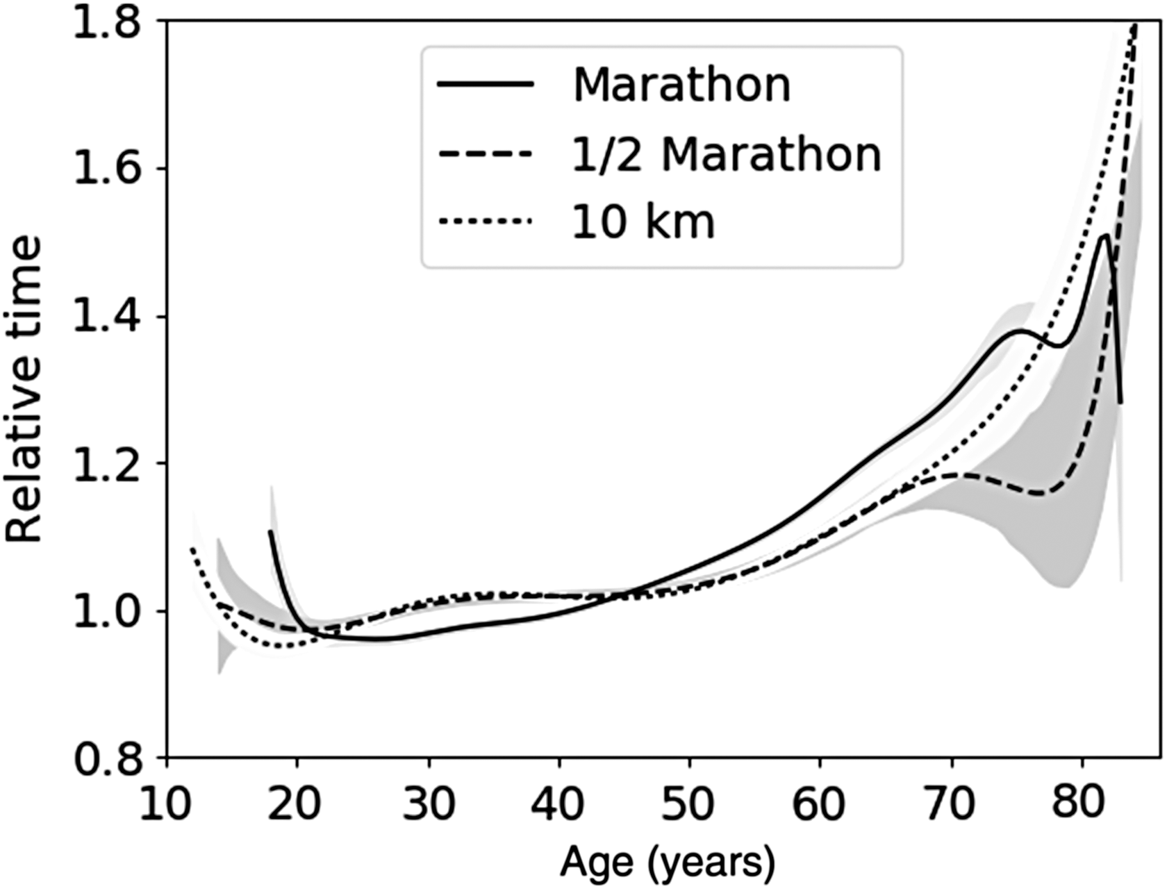
Model for dependence between age and performance on the different distances for men. The shaded areas denote the 95% confidence intervals.

FIG. 4.

Model for dependence between age and performance on the different distances for women. The shaded areas denote the 95% confidence intervals.

Although the primary goal is to use this model for compensating for age effects in the Subgroup Discovery experiments that are described in the Subgroup Discovery section of the Results, the models itself also give already some interesting insights. First of all, we notice that in the reliable age range from roughly 20–60 years, the models on all distances are very similar for both men and women. This is in agreement with a previous study that used the results of the New York marathon,³⁴ where the authors conclude that there are no physiological differences between men and women in age-related declines for marathon running.

Moreover, in the reliable age range, the difference between our models for the 10 km and the half marathon is negligible. The model for the full marathon is mainly different for ages more than 50, where compared with the shorter distances, the performance of the runners decreases more rapidly. Finally, on all distances, there are mainly two different regimens. For athletes younger than 50, the relative time is approximately constant for the two shortest distances and slightly increasing for the full marathon. The relative time of athletes older than 50 increases more steeply. The distinction between the two different regimens for athletes older or younger than roughly 50 years is found previously.³⁵ However, contrary to this study, we find that the rate of decline for men is more than that of women.

Finally, we also performed a lack-of-fit F test to determine the statistical significance of the models.³⁶ We have tested the null hypothesis that there is no lack of fit and thus the model properly fits the data. Therefore, we calculated the value of the following F-statistic: \documentclass{aastex}\usepackage{amsbsy}\usepackage{amsfonts}\usepackage{amssymb}\usepackage{bm}\usepackage{mathrsfs}\usepackage{pifont}\usepackage{stmaryrd}\usepackage{textcomp}\usepackage{portland, xspace}\usepackage{amsmath, amsxtra}\usepackage{upgreek}\pagestyle{empty}\DeclareMathSizes{10}{9}{7}{6}\begin{document} \begin{align*} F = { \frac { N - n } { n - d - 1 } } { \frac { { \rm { SSLF } } } { { \rm { SSPE } } } } , \end{align*} \end{document}

where N is the total number of datapoints, n is the number of distinct ages, and d is the polynomial degree of the model. Moreover, sum of squares due to lack of fit (SSLF) and sum of squares due to the pure error (SSPE) are the SSE due to lack of fit and the SSE due to the pure error, respectively. Therefore, this F-statistic describes the fraction of the total error that is due to the variation present at every age.

The sum of these two quantities is equal to the total sum of squares of errors, that is, the sum of squares of all residuals. More precisely, \documentclass{aastex}\usepackage{amsbsy}\usepackage{amsfonts}\usepackage{amssymb}\usepackage{bm}\usepackage{mathrsfs}\usepackage{pifont}\usepackage{stmaryrd}\usepackage{textcomp}\usepackage{portland, xspace}\usepackage{amsmath, amsxtra}\usepackage{upgreek}\pagestyle{empty}\DeclareMathSizes{10}{9}{7}{6}\begin{document} \begin{align*} { \rm{SSE}} = { \rm{SSLF}} + { \rm{SSPE}} \\= \mathop \sum \limits_{i = 1}^n { \rm{ }}{n_i}{ \left( { \bar t_{{ \rm{rel}}}^i - \left\langle {t_{{ \rm{rel}}}^i} \right\rangle } \right) ^2} + \mathop \sum \limits_{i = 1}^n { \rm{ }} \mathop \sum \limits_{j = 1}^{{n_i}} { \rm{ }}{ \left( {t_{{ \rm{rel}}}^{i , j} - \bar t_{{ \rm{rel}}}^i} \right) ^2} , \end{align*} \end{document}

where n_i is the number of athletes with a certain age x_i, \documentclass{aastex}\usepackage{amsbsy}\usepackage{amsfonts}\usepackage{amssymb}\usepackage{bm}\usepackage{mathrsfs}\usepackage{pifont}\usepackage{stmaryrd}\usepackage{textcomp}\usepackage{portland, xspace}\usepackage{amsmath, amsxtra}\usepackage{upgreek}\pagestyle{empty}\DeclareMathSizes{10}{9}{7}{6}\begin{document} $$\bar t_{{ \rm{rel}}}^i$$ \end{document} is the average relative time of the runners with this age, \documentclass{aastex}\usepackage{amsbsy}\usepackage{amsfonts}\usepackage{amssymb}\usepackage{bm}\usepackage{mathrsfs}\usepackage{pifont}\usepackage{stmaryrd}\usepackage{textcomp}\usepackage{portland, xspace}\usepackage{amsmath, amsxtra}\usepackage{upgreek}\pagestyle{empty}\DeclareMathSizes{10}{9}{7}{6}\begin{document} $$\left\langle {t_{{ \rm{rel}}}^i} \right\rangle$$ \end{document} is the predicted relative time of the model at age x_i, and \documentclass{aastex}\usepackage{amsbsy}\usepackage{amsfonts}\usepackage{amssymb}\usepackage{bm}\usepackage{mathrsfs}\usepackage{pifont}\usepackage{stmaryrd}\usepackage{textcomp}\usepackage{portland, xspace}\usepackage{amsmath, amsxtra}\usepackage{upgreek}\pagestyle{empty}\DeclareMathSizes{10}{9}{7}{6}\begin{document} $$t_{{ \rm{rel}}}^{i , j}$$ \end{document} is the relative time of an athlete.

For each distance, male and female athletes, we used the F-statistic to calculate a p-value. This p-value is the probability that we get this value for the F-statistic given that the null hypothesis is true, that is, there is no lack-of-fit. Thus, roughly speaking, the p-value is the probability that the model correctly describes the relationship between age and performance. In Table 2, we display p-values for models on different distances. From the results in this table, we see that for each distance, there is a substantially large probability that we find a situation as extreme as present in this data collection. Hence, for all distances with no substantial evidence, there is lack of fit. Therefore, we can assume that our models are an appropriate description for the relationship between age and performance.

Table 2.

The p-values for the models on the different distances for male and female athletes

	10 km	Half marathon	Full marathon
Men	0.15	0.75	0.18
Women	0.44	0.88	0.50

These values correspond to the probability that we have a situation as extreme as encountered in this article, assuming that the model correctly describes the relationship between age and performance.

Pacing profiles

As mentioned at the end of Materials section, we used the relative paces between two successive intermediate points to define the three most characteristic pacing profiles. In this section, we discuss those different profiles in more detail and also elaborate on the relationship between pacing profile and performance during the race. Since qualitative behavior is similar for men and women, we first focus on men and then briefly mention the differences with women.

The results about the pacing profiles are displayed in Figure 5. First, we focus on the three figures on the left-hand side of Figure 5. In these figures, the three most characteristic pacing profiles are displayed. We observe that in the 10 km race (top row), the three most common pacing profiles are negative pacing, even pacing, and positive pacing. Thus, there are runners who increase their pace, run constant, or slow down, respectively. If we look at the half marathon (middle row), we find that there are a group of athletes who slightly increase their pace and two groups that slowed down as the race progresses.

FIG. 5.

Three most characteristic pacing profiles and the relationship with the performance for men on three different distances. The first, second, and third rows are for the 10 km, half marathon, and full marathon, respectively. The figures on the left-hand side show the most characteristic pacing profiles and the figures on the right display the fraction of athletes with each of the three profiles as a function of the relative time. For the relative pace, we show the pace halfway to two successive intermediate points and the relative times are grouped in bins with size 0.05. The shading in the figures on the right-hand side represents the fraction of athletes who have the pacing profile with the corresponding line color in the figure to the left.

The difference between the latter two is the amount that the runners slow down. Moreover, runners with negative pacing only slightly increase their pace, and therefore, the athletes in this group approximately run at a constant pace. Finally, in the full marathon (bottom row), all three profiles are positive pacing and the differences are again in the level of speed drop during the race. Thus, on longer distances there is less variation in type of pacing profiles and more runners have a positive pacing profile.

Up to now, we have only considered male runners. For women, the information about the pacing profiles is very similar. Only for the full marathon, there are some small quantitative differences. We obtain that the negative change in speed for the three positive pacing profiles is larger for male runners than for women. Hence, in the full marathon, we find that women start more conservatively than men.

It is also interesting to investigate the relationship between pacing profile and performance in the race. Therefore, we now focus on the three figures on the right-hand side of Figure 5. We find on all three distances that the profile with the highest starting relative pace at the beginning of the race, that is, the darkest area in Figure 5, is less common under athletes with a small relative time. There is only a very small fraction of runners who have this pacing profile and end up with a relative time below 1. Moreover, we observe that this profile becomes more and more present for athletes with a larger relative time.

If we look more closely at the runners with relative times around one or smaller, we find in the 10 km that the group is dominated by athletes who run at a constant pace. For the half marathon, these athletes can be roughly divided into two groups of equal size. The group that runs with a small negative split and the runners who have a small positive split. In the full marathon, the picture is rather clear and almost all athletes with a small relative time have the most conservative pacing profile with the smallest overall change in pace. For women, the results are again very similar and there are only some small quantitative differences.

Subgroup Discovery

In the Pacing profiles section of the Results, we have shown that there is a strong relationship between the pacing profile and the final performance in a race. However, there are also other factors that influence the final result in a race. Here, we discuss the results of the experiments with Subgroup Discovery to find race-specific features that have the largest impact on race performance for different distances.

Since we are only interested in race-specific properties, we want to compensate for age effects. We consider a regression setting, where the target variable is the relative difference between the relative time of an athlete and the time that is predicted by the age-performance model. For each distance, we treat men and women separately.

If we consider all male runners, the average difference between the model and the actual performance is \documentclass{aastex}\usepackage{amsbsy}\usepackage{amsfonts}\usepackage{amssymb}\usepackage{bm}\usepackage{mathrsfs}\usepackage{pifont}\usepackage{stmaryrd}\usepackage{textcomp}\usepackage{portland, xspace}\usepackage{amsmath, amsxtra}\usepackage{upgreek}\pagestyle{empty}\DeclareMathSizes{10}{9}{7}{6}\begin{document} $$ - 0.00008{ \rm{ \% }}$$ \end{document} , \documentclass{aastex}\usepackage{amsbsy}\usepackage{amsfonts}\usepackage{amssymb}\usepackage{bm}\usepackage{mathrsfs}\usepackage{pifont}\usepackage{stmaryrd}\usepackage{textcomp}\usepackage{portland, xspace}\usepackage{amsmath, amsxtra}\usepackage{upgreek}\pagestyle{empty}\DeclareMathSizes{10}{9}{7}{6}\begin{document} $$- 0.00002{ \rm{ \% }}$$ \end{document} , and \documentclass{aastex}\usepackage{amsbsy}\usepackage{amsfonts}\usepackage{amssymb}\usepackage{bm}\usepackage{mathrsfs}\usepackage{pifont}\usepackage{stmaryrd}\usepackage{textcomp}\usepackage{portland, xspace}\usepackage{amsmath, amsxtra}\usepackage{upgreek}\pagestyle{empty}\DeclareMathSizes{10}{9}{7}{6}\begin{document} $$- 0.00002{ \rm{ \% }}$$ \end{document} for the 10 km, half marathon, and full marathon, respectively. For all women, this is on average equal to \documentclass{aastex}\usepackage{amsbsy}\usepackage{amsfonts}\usepackage{amssymb}\usepackage{bm}\usepackage{mathrsfs}\usepackage{pifont}\usepackage{stmaryrd}\usepackage{textcomp}\usepackage{portland, xspace}\usepackage{amsmath, amsxtra}\usepackage{upgreek}\pagestyle{empty}\DeclareMathSizes{10}{9}{7}{6}\begin{document} $$- 0.00002{ \rm{ \% }}$$ \end{document} , \documentclass{aastex}\usepackage{amsbsy}\usepackage{amsfonts}\usepackage{amssymb}\usepackage{bm}\usepackage{mathrsfs}\usepackage{pifont}\usepackage{stmaryrd}\usepackage{textcomp}\usepackage{portland, xspace}\usepackage{amsmath, amsxtra}\usepackage{upgreek}\pagestyle{empty}\DeclareMathSizes{10}{9}{7}{6}\begin{document} $$ - 0.01{ \rm{ \% }}$$ \end{document} , and \documentclass{aastex}\usepackage{amsbsy}\usepackage{amsfonts}\usepackage{amssymb}\usepackage{bm}\usepackage{mathrsfs}\usepackage{pifont}\usepackage{stmaryrd}\usepackage{textcomp}\usepackage{portland, xspace}\usepackage{amsmath, amsxtra}\usepackage{upgreek}\pagestyle{empty}\DeclareMathSizes{10}{9}{7}{6}\begin{document} $$- 0.00005{ \rm{ \% }}$$ \end{document} . The minus sign indicates that athletes are faster than predicted. Hence, we are looking for subgroups of substantial size, where the runners on average perform sufficiently better than these numbers of the entire group.

In this research, we have used a beam search strategy with width 10. The numerical search strategy setting is best-bins with 128 bins. This implies that on each subsequent level, we considered the 10 subgroups with the highest quality. Moreover, the numerical attributes were binned in 128 bins. For these attributes, all numerical values were considered and the values that gave the optimal split were selected. The quality measure used is Explained Variance R².³⁷ The advantage of this measure is that it considers both the distribution properties of the subgroup and the complement. The value of R² ranges between 0 and 1, where higher values correspond to subgroups of better quality. The subgroups of highest quality for men and women are shown in Tables 3 and 4, respectively. Below we discuss the results of depth 1 and 2 separately.

Table 3.

Characteristics of optimal subgroups for men on the different distances

Distance	Depth	Description	Size	Average (%)	R ²
10 km	1	Min. pace change ≥−5.40%	6028	−3.61	0.125
10 km	2	Min. pace change ≥−5.40% \documentclass{aastex}\usepackage{amsbsy}\usepackage{amsfonts}\usepackage{amssymb}\usepackage{bm}\usepackage{mathrsfs}\usepackage{pifont}\usepackage{stmaryrd}\usepackage{textcomp}\usepackage{portland, xspace}\usepackage{amsmath, amsxtra}\usepackage{upgreek}\pagestyle{empty}\DeclareMathSizes{10}{9}{7}{6}\begin{document} $$\wedge$$ \end{document} Difference max. and min. pace change ≤9.20%	5605	−4.46	0.143
1/2 marathon	1	Min. pace change ≥−8.39%	5242	−4.28	0.160
1/2 marathon	2	Distance of slow start pacing profile ≤0.191 \documentclass{aastex}\usepackage{amsbsy}\usepackage{amsfonts}\usepackage{amssymb}\usepackage{bm}\usepackage{mathrsfs}\usepackage{pifont}\usepackage{stmaryrd}\usepackage{textcomp}\usepackage{portland, xspace}\usepackage{amsmath, amsxtra}\usepackage{upgreek}\pagestyle{empty}\DeclareMathSizes{10}{9}{7}{6}\begin{document} $$\wedge$$ \end{document} Min. pace change ≥−8.65%	5171	−4.44	0.164
Full marathon	1	Interquartile range pace change ≤7.47%	24,824	−5.94	0.254
Full marathon	2	Interquartile range pace change ≤7.47% \documentclass{aastex}\usepackage{amsbsy}\usepackage{amsfonts}\usepackage{amssymb}\usepackage{bm}\usepackage{mathrsfs}\usepackage{pifont}\usepackage{stmaryrd}\usepackage{textcomp}\usepackage{portland, xspace}\usepackage{amsmath, amsxtra}\usepackage{upgreek}\pagestyle{empty}\DeclareMathSizes{10}{9}{7}{6}\begin{document} $$\wedge$$ \end{document} Pace change 0–21 km to 21–30 km ≥−12.3%	22,497	−7.25	0.285

We give the description, size of the subgroup, and distributional properties of the athletes who are part of this subgroup at search depth 1 and 2. Finally, we also specify the value for the quality measure R² in the last column.

Table 4.

Overview of optimal subgroups for women on the different distances

Distance	Depth	Description	Size	Average (%)	R ²
10 km	1	Min. pace change ≥−4.71%	7050	−4.58	0.143
10 km	2	Min. pace change ≥−4.71% \documentclass{aastex}\usepackage{amsbsy}\usepackage{amsfonts}\usepackage{amssymb}\usepackage{bm}\usepackage{mathrsfs}\usepackage{pifont}\usepackage{stmaryrd}\usepackage{textcomp}\usepackage{portland, xspace}\usepackage{amsmath, amsxtra}\usepackage{upgreek}\pagestyle{empty}\DeclareMathSizes{10}{9}{7}{6}\begin{document} $$\wedge$$ \end{document} Difference max. and min. pace change ≤8.69%	6610	−5.28	0.158
1/2 marathon	1	Distance of slow start pacing profile ≤0.151	5816	−4.66	0.176
1/2 marathon	2	Distance of slow start pacing profile ≤0.151 \documentclass{aastex}\usepackage{amsbsy}\usepackage{amsfonts}\usepackage{amssymb}\usepackage{bm}\usepackage{mathrsfs}\usepackage{pifont}\usepackage{stmaryrd}\usepackage{textcomp}\usepackage{portland, xspace}\usepackage{amsmath, amsxtra}\usepackage{upgreek}\pagestyle{empty}\DeclareMathSizes{10}{9}{7}{6}\begin{document} $$\wedge$$ \end{document} Difference max. and min. pace change ≤11.4%	5453	−5.19	0.184
Full marathon	1	Standard deviation pace change ≤4.48%	19,303	−6.03	0.271
Full marathon	2	Standard deviation pace change ≤4.48% \documentclass{aastex}\usepackage{amsbsy}\usepackage{amsfonts}\usepackage{amssymb}\usepackage{bm}\usepackage{mathrsfs}\usepackage{pifont}\usepackage{stmaryrd}\usepackage{textcomp}\usepackage{portland, xspace}\usepackage{amsmath, amsxtra}\usepackage{upgreek}\pagestyle{empty}\DeclareMathSizes{10}{9}{7}{6}\begin{document} $$\wedge$$ \end{document} Pace change 0–5 km to 5–35 km ≥ −11.9%	18,399	−6.55	0.282

The characteristics that are shown for men in Table 3 also occur here.

Individual features

For men, we find that on the 10 km and the half marathon, the best subgroup consists of athletes who limit their speed drop during the race. Finally, for the full marathon, the fast finishers have small fluctuations in the acceleration throughout the race. Note that the athletes in the best subgroups perform on average \documentclass{aastex}\usepackage{amsbsy}\usepackage{amsfonts}\usepackage{amssymb}\usepackage{bm}\usepackage{mathrsfs}\usepackage{pifont}\usepackage{stmaryrd}\usepackage{textcomp}\usepackage{portland, xspace}\usepackage{amsmath, amsxtra}\usepackage{upgreek}\pagestyle{empty}\DeclareMathSizes{10}{9}{7}{6}\begin{document} $$3.61{ \rm{ \% }}$$ \end{document} , \documentclass{aastex}\usepackage{amsbsy}\usepackage{amsfonts}\usepackage{amssymb}\usepackage{bm}\usepackage{mathrsfs}\usepackage{pifont}\usepackage{stmaryrd}\usepackage{textcomp}\usepackage{portland, xspace}\usepackage{amsmath, amsxtra}\usepackage{upgreek}\pagestyle{empty}\DeclareMathSizes{10}{9}{7}{6}\begin{document} $$4.28{ \rm{ \% }}$$ \end{document} , and \documentclass{aastex}\usepackage{amsbsy}\usepackage{amsfonts}\usepackage{amssymb}\usepackage{bm}\usepackage{mathrsfs}\usepackage{pifont}\usepackage{stmaryrd}\usepackage{textcomp}\usepackage{portland, xspace}\usepackage{amsmath, amsxtra}\usepackage{upgreek}\pagestyle{empty}\DeclareMathSizes{10}{9}{7}{6}\begin{document} $$5.94{ \rm{ \% }}$$ \end{document} better than the result of the age-performance model for the 10 km, half marathon, and full marathon, respectively. Thus, on average, the athletes in these subgroups perform substantially better than all participants.

For women, we obtain similar descriptions for the best subgroups compared with men on the 10 km and the full marathon. On the half marathon, the best subgroups are different for men and women. However, for men, the second best subgroup on the half marathon is runners with a distance to slow start pacing profile ≤0.190 ( \documentclass{aastex}\usepackage{amsbsy}\usepackage{amsfonts}\usepackage{amssymb}\usepackage{bm}\usepackage{mathrsfs}\usepackage{pifont}\usepackage{stmaryrd}\usepackage{textcomp}\usepackage{portland, xspace}\usepackage{amsmath, amsxtra}\usepackage{upgreek}\pagestyle{empty}\DeclareMathSizes{10}{9}{7}{6}\begin{document} $${R^2} = 0.153$$ \end{document} ). The quality of this subgroup is almost as high as the quality of the best subgroup ( \documentclass{aastex}\usepackage{amsbsy}\usepackage{amsfonts}\usepackage{amssymb}\usepackage{bm}\usepackage{mathrsfs}\usepackage{pifont}\usepackage{stmaryrd}\usepackage{textcomp}\usepackage{portland, xspace}\usepackage{amsmath, amsxtra}\usepackage{upgreek}\pagestyle{empty}\DeclareMathSizes{10}{9}{7}{6}\begin{document} $${R^2} = 0.160$$ \end{document} ). For women, the second best subgroup has the description that the minimum pace change ≥ −8.0% \documentclass{aastex}\usepackage{amsbsy}\usepackage{amsfonts}\usepackage{amssymb}\usepackage{bm}\usepackage{mathrsfs}\usepackage{pifont}\usepackage{stmaryrd}\usepackage{textcomp}\usepackage{portland, xspace}\usepackage{amsmath, amsxtra}\usepackage{upgreek}\pagestyle{empty}\DeclareMathSizes{10}{9}{7}{6}\begin{document} $$\left( {{R^2} = 0.176} \right)$$ \end{document} . Thus, also for this distance, the results are very similar for men and women, and there are only some small quantitative differences. Note that also for women, there is a considerable difference in the performance of the runners in the best subgroups and all female participants.

Hence, we can conclude that rather than the pace itself, it is more important to focus on the pace changes during the race. For shorter distances, it is enough to limit the amount of deceleration. Whereas for the full marathon, there is a bigger restriction on the pace changes. Namely, the fluctuations in the pace changes throughout the race should be sufficiently small.

Multiple features

Instead of considering subgroups with single conditions, we also have investigated the best subgroups at depth \documentclass{aastex}\usepackage{amsbsy}\usepackage{amsfonts}\usepackage{amssymb}\usepackage{bm}\usepackage{mathrsfs}\usepackage{pifont}\usepackage{stmaryrd}\usepackage{textcomp}\usepackage{portland, xspace}\usepackage{amsmath, amsxtra}\usepackage{upgreek}\pagestyle{empty}\DeclareMathSizes{10}{9}{7}{6}\begin{document} $$d = 2$$ \end{document} . Therefore, we extended our search to subgroups that are described by two conditions.

On the 10 km, the results are comparable for men and women. On top of the condition that already came forward in the search at depth 1, we find that the difference between the maximum and minimum pace change should be small. Since for these distances the distribution of pace changes only consists of two pace changes, this condition is equivalent to having small fluctuations in pace changes throughout the race.

For the two longest distances, the result for men and women is slightly different. For the half marathon, both subgroups are described by an upper limit on the distance to the slow start pacing profile, but the second condition is different. The female runners have an additional restriction on the difference between the maximum and minimum pace change. On the contrary, for males, there is a lower bound on the pace change. On the full marathon, the results are qualitatively similar as they consist of a condition on the fluctuations in the pace changes and a condition on the pace change between two specific intervals. For men, there is a restriction on the interquartile range of the pace changes and the pace change from the first half of the full marathon to the interval from 21 to 30 km. On the contrary, for women, the conditions are on the standard deviation of the page changes and the change in pace from the first 5 km to the interval from 5 to 35 km.

By extending our search to depth 2, the qualities of the best subgroups are maximally roughly 15% higher. Thus, there is some improvement in the quality of the optimal subgroups, but it is not very large. If we extend the search depth even further, this improvement will become even smaller. Therefore, we do not go beyond search depth 2.

Statistical significance

In Subgroup Discovery, a large number of candidate subgroups are considered, and therefore, many hypotheses are tested. Therefore, there is a risk of finding a result simply because such a large number of hypotheses are tested. To overcome this problem, we validated our results by making use of a distribution of false discoveries.³⁸ By using swap-randomization on the target attribute, we have calculated the threshold for finding a statistically significant result. The results for a significance level \documentclass{aastex}\usepackage{amsbsy}\usepackage{amsfonts}\usepackage{amssymb}\usepackage{bm}\usepackage{mathrsfs}\usepackage{pifont}\usepackage{stmaryrd}\usepackage{textcomp}\usepackage{portland, xspace}\usepackage{amsmath, amsxtra}\usepackage{upgreek}\pagestyle{empty}\DeclareMathSizes{10}{9}{7}{6}\begin{document} $$\alpha = 0.05$$ \end{document} are displayed in Table 5. Hence, the qualities of the presented subgroups are far above these thresholds, and therefore, we can conclude that our results are statistically significant.

Table 5.

Lower bounds for the explained variance R² for subgroups at search depth 1 and 2 to be statistically significant at level α = 0.05

	Depth	10 km	Half marathon	Full marathon
Men	1	0.00171	0.00197	0.000497
Men	2	0.00321	0.00316	0.000844
Women	1	0.00135	0.00145	0.000624
Women	2	0.00229	0.00264	0.00106

Conclusions

In this article, we have used a data-driven approach to investigate several properties that affect the performance of an athlete in a long-distance running event. We have used public data of races on the 10 km, half marathon, and full marathon organized by the Boston Athletic Association in the years 2015–2017.

First, we have developed distance- and gender-specific models for describing the relationship between age and performance. In these models, the differences between men and women as well as the differences between the models for the 10 km and the half marathon are negligible. However, the model for the full marathon is different. Namely, the rate of decline in performance for ages above 50 is bigger on the full marathon than on the 2 shorter distances.

Second, for every distance, we have identified the three most characteristic pacing profiles for men and women. By looking at the fraction of athletes who have one of these specific pacing profiles as a function of the final relative time, we have found that only a very small part of the fast athletes have a pacing profile with the largest decrease in pace. Furthermore, we have obtained that even pacing is the dominant profile among the fast finishers in the 10 km. For the half marathon, there are an equal number of good performing runners who have either small negative or positive pacing. Finally, for the full marathon, the three most characteristic pacing profiles are all positive pacing. The profile with the smallest speed drop throughout the race is the most dominant pacing profile among the group of fast athletes. These results hold for both men and women.

Finally, since the property for having the best possible performance in a race is still unknown, we have transformed raw data into multiple features that characterize pacing throughout the race. After compensating for age effects by using the age-performance models, we have used Subgroup Discovery to select the pacing properties that have the largest impact on performance. We have found that controlling pace changes is the most important feature for performance. On the 10 km, on average men perform 4.46% better than the prediction of the age-performance model if the minimum pace change is larger than −5.40% and the difference between the maximum and minimum pace change is smaller than 9.20%. For women, similar conditions with slightly different numbers hold. On the half marathon, we find that male athletes perform 4.44% better than predicted, if the runners roughly have a small negative pacing profile and the minimum pace change is larger than −8.65%. The female athletes perform 5.19% better than predicted, if the runners also approximately have a small negative pacing profile and the difference between the maximum and minimum pace change is smaller than 11.4%.

On the full marathon, there are only quantitative differences for the optimal subgroups for men and women. For men, we have found that they on average perform 7.25% better than the model predicts, if the interquartile range of the pace changes is smaller than 7.47% and the pace change from 0–21 km to 21–30 km is larger than −12.3%. For women, we have obtained that runners on average perform 6.55% better than the prediction of the age-performance model, if the standard deviation of the pace changes is smaller than 4.48% and the pace change from 0–5 km to 5–35 km is larger than −11.9%. This shows that pacing has a large impact on the result in long-distance running event, and thus, besides physiological properties, is probably one of the biggest factors in running performances.

In comparison with most previous studies on pacing strategies in long-distance running, we have used a data-driven approach instead of focusing on a small set of runners or addressing pacing in an experimental setting.^39–42 The big advantage of this approach is that this study concerns a much larger set and therefore many more different patterns can be investigated and tested simultaneously in comparison with a more controlled setting. However, the downside of this data-driven approach is that some important information is unknown, such as the preparation before a race and the reason for running the race, and therefore cannot be taken into account. In our approach, the only external factor we have is age, which we corrected for by using the age-performance models. For data sets with information on other external factors, such as the previously mentioned examples, these factors can be incorporated by introducing additional parameters in our model. Given how easily we can adapt the modeling approach, we can simply adapt a multidimensional regression of the relationship between the performance and all known external factors. In this case, the model would incorporate the information about the external factors, and therefore, the information about these external factors would also be included in the definition of fast finisher and underperformers. For future research, it would be interesting to perform this data-driven approach with a data set where more external factors than age are known. In this manner, we could compare the results and investigate the importance of the different external factors.

We believe that the data and methods we have used in this study lead to a good representative to generalize the results to other running events. Nevertheless, for the 10 km and half marathon there are only two intermediate times. Therefore, the data collection is quite restricted and the information about the pacing on these distances is limited. Including more intermediate times would definitely give more detailed information about the optimal pacing.

The results obtained in this research give concrete and relatively simple conditions on the pacing during a race. This could be highly valuable information for coaches to help professional and recreational runners to optimize their performance. For future studies, it is worthwhile to collect data of multiple races of individual athletes. With the methods used in this research, we could give an athlete personalized advice about his or her ideal pacing strategy.

Footnotes

Acknowledgments

It is a pleasure to thank Prof. Dr. Joost Kok and the organizers of the Leiden Marathon for useful discussions. We are also grateful to the Boston Athletic Association for giving us permission to use the data.

Author Disclosure Statement

No competing financial interests exist.

Abbreviations Used

References

Asics. Reasons to run. Hoofddorp: Asics Europe. 2009.

Running & Jogging-Statistics & Facts. https://www.statista.com/topics/1743/running-and-jogging (last accessed June 2018 ).

Trappe

Marathon runners: How do they age?. Sports Med. 2007; 37:302–305.

Tanaka

, Seals

. Endurance exercise performance in Masters athletes: Age-associated changes and underlying physiological mechanisms. J Physiol. 2008; 586:55–63.

Knechtle

, Rüst

, Rosemann

, Lepers

. Age-related changes in 100-km ultra-marathon running performance. Age. 2012; 34:1033–1045.

Lara

, Salinero

, Del Coso

. The relationship between age and running time in elite marathoners is U-shaped. Age. 2014; 36:1003–1008.

Schulz

, Curnow

. Peak performance and age among superathletes: Track and field, swimming, baseball, tennis and golf. J Gerontol. 1988; 43:113–120.

Wiswell

, Jaque

, Marcell

, et al. Maximal aerobic power, lactate threshold, and running performance in master athletes. Med Sci Sports Exerc. 2000; 32:1165–1170.

Foster

, Snyder

, Thompson

, et al. Effect of pacing strategy on cycle time trial performance. Med Sci Sports Exerc. 1993; 25:383–388.

10.

Abbiss

, Laursen

. Describing and understanding pacing strategies during athletic competition. Sports Med. 2008; 38:239–252.

11.

Skorski

, Abbiss

. The manipulation of pace within endurance sport. Front Physiol. 2017; 8:10–2.

12.

De Koning

, Foster

, Bakkum

, et al. Regulation of pacing strategy during athletic competition. PLoS ONE. 2011; 6:e1586–3.

13.

Hanley

Pacing and sex-based differences in Olympic and IAAF World Championship marathons. J Sport Sci. 2016; 34:1675–1681.

14.

Dáz

, Fernández-Ozcorta

, Santos-Concejero

. The influence of pacing strategy on marathon world records. Eur J Sport Sci. 2018; 18:781–786.

15.

Theodoros

, Knechtle

. Effect of age and performance on pacing of marathon runners. J Sports Med. 2017; 8:171–180.

16.

Santos-Lozano

, Collado

, Foster

, et al. Influence of sex and level on marathon pacing strategy. Insights from the New York City Race. Int J Sports Med. 2014; 35:933–938.

17.

Boston Athletic Association. www.baa.org (last accessed April 2018 ).

18.

Ely

, Cheuvront

, Roberts

, Montain

. Impact of weather on marathon-running performance. Med Sci Sports Exerc. 2007; 39:487–493.

19.

Vihma

Effects of weather on the performance of marathon runners. Int J Biometeorol. 2010; 54:297–306.

20.

El Helou

, Tafflet

, Berthelot

, et al. Impact of environmental parameters on marathon running performance. PLoS ONE. 2012; 7:e3740–7.

21.

Lane

, Scott

, Hebl

, et al. Introduction to Statistics. Online edition. Available online at www.onlinestatbook.com/Online_Statistics_Education.pdf (last accessed June 2018 ).

22.

Chiang

MM-T

, Mirkin

. Intelligent choice of the number of clusters in k-Means clustering: An experimental study with different cluster spreads. J Classif. 2010; 27:3–40.

23.

Klösgen

, Zytkow

. Handbook of data mining and knowledge discovery. New York, NY: Oxford University Press, Inc. 2002.

24.

Novak

, Lavrač

, Webb

. Supervised descriptive rule discovery: A unifying survey of contrast set, emerging pattern and subgroup mining. J Mach Learn Res. 2009; 10:377–403.

25.

Grosskreutz

, Rüping

. On subgroup discovery in numerical domains. Data Min Knowl Discov. 2009; 19:210–226.

26.

Atzmüller

, Lemmerich

Fast subgroup discovery for continuous target concepts. In: ISMIS, The International Symposium on Methodologies for Intelligent Systems, 2009. pp. 35–44.

27.

Geisser

. Predictive inference: An introduction. New York, NY: Chapman and Hall. 1993.

28.

Geng

, Hamilton

. Interestingness measures for data mining: A survey. ACM Comput Surv. 2006; 38.

29.

Jorge

, Azevedo

, Pereira

Distribution rules with numeric attributes of interest. PKDD, The European Conference on Principles and Practice of Knowledge Discovery in Databases. Berlin, Germany, 2006, pp. 247–258.

30.

Pieters

BFI

, Knobbe

, Džeroski

Subgroup discovery in ranked data, with an application to gene set enrichment. Preference learning 2010 at ECML PKDD, The European Conference on Machine Learning and Principles and Practice of Knowledge Discovery in Databases. Barcelona, Spain, 2010.

31.

Meeng

, Knobbe

. Flexible enrichment with Cortana-software demo. BeneLearn, the Annual Belgian-Dutch Conference on Machine Learning. The Hague, The Netherlands, 2011, pp. 117–119.

32.

Fox

. Applied regression analysis and generalized linear models. Thousand Oaks, CA: Sage Publications, Inc. 2015.

33.

Donato

AJ.

Declines in physiological functional capacity with age: A longitudinal study in peak swimming performance. J Appl Physiol. 2003; 94:764–769.

34.

Lepers

, Cattagni

. Do older athletes reach limits in their performance during marathon running?. Age. 2012; 34:773–781.

35.

Tanaka

, Seals

. Invited review: Dynamic exercise performance in Masters athletes: Insight into the effects of primary human aging on physiological functional capacity. J Appl Physiol. 2003; 95:2152–2162.

36.

Brook Richard

, Arnold Gregory

Applied regression analysis and experimental design. CRC Press. 1985.

37.

Knobbe

, Orie

, Hofman

, et al. Sports analytics for professional speed skating. Data Min Knowl Disc. 2017; 31:1872–1902.

38.

Duivesteijn

, Knobbe

. Exploiting false discoveries–statistical validation of patterns and quality measures in subgroup discovery. ICDM, The International Conference on Data Mining. Vancouver, Canada, 2011. pp. 151–160.

39.

Maughan

, Leiper

, Thompson

. Rectal temperature after marathon running. Br J Sports Med. 1985; 19:192–195.

40.

Lambert

, Dugas

, Kirkman

, et al. Changes in running speeds in a 100 KM ultra-marathon race. J Sports Sci Med. 2004; 3:167–173.

41.

Gosztyla

, Edwards

, Quinn

, Kenefick

. The impact of different pacing strategies on five-kilometer running time trial performances. J Strength Cond Res. 2006; 20:882–886.

42.

March

, Vanderburgh

, Titlebaum

, Hoops

. Age, sex, and finish time as determinants of pacing in the marathon. J Strength Cond Res. 2011; 25:386–391.