Seasonal Linear Predictivity in National Football Championships

Abstract

Predicting the results of sport matches and competitions is a growing research field, benefiting from the increasing amount of available data and novel data analytics techniques. Excellent forecasts can be achieved by advanced statistical and machine learning methods applied to detailed historical data, especially in very popular sports such as football (soccer). Here, we show that despite the large number of confounding factors, the results of a football team in longer competitions (e.g., a national league) follow a basically linear trend that is also useful for predictive purposes. In support of this claim, we present a set of experiments of linear regression compared to alternative approaches on a database collecting the yearly results of 746 teams playing in 22 divisions spanning up to five different levels from 11 countries, in 25 football seasons, for a total of 181,160 matches grouped in 9386 seasonal time series.

Introduction

Predicting sport results in the last few years has ceased being just an art for initiated specialists¹ to enter the realm of data analytics, thus providing a further support to the claim of considering as science many aspects of several sports.^2–4 In particular, interest in forecasting the results of sporting competitions has grown in the last few years, essentially because of two key factors: the arising need for more reliable predictive models by betting agencies^5–10 and the increasing number of available sources collecting data at different levels of detail. However, the predictability of results is still a debated issue,^11–15 mainly because of the random effects affecting the outcome of a match, with football (soccer) as a major example.^16–21 Clearly, structural effects have an even larger impact: as noted by Parasich,²² the average precision (53%) reached by bookmakers in forecasting the outcome of a match (home win, draw, away win) seems not so positive anymore if you consider that the home team wins 46% of matches, and thus the null constant model always predicting a home win achieves 46% precision.

Many algorithms from statistics^* and machine learning have recently been used to overcome such randomness bias in order to achieve good predictive performance, which have been applied to data catching diverse aspects of the game, with different historical spans, or at various levels of detail, even publicly available online as infotainment resources.^† Generalized linear or polynomial models and logistic or probit regressions have been used in the literature since the mid-2000s,^9,15,23–31 using as variables points or goals or even adding economic parameters. More recent are statistical approaches based on Bayesian or Poissonian predictors,^{10,21,32–43} or even Weibull counts,^44,45 where individual player's performance is also included as a model covariate. Further statistical approaches involving for instance Markov chain Monte Carol, hierarchical models, or moving averages have been published,^8,46–52 indicating that a shared agreement on a grounded modeling is still far from being acknowledged. More recently, machine learning models have become a major trend in the field, and all the best-known algorithms have appeared on the football forecasting arena (e.g., nearest neighbours, Gaussian and Poisson processes, Random Forest, Support Vector Machines, MultiLayer Perceptron just to name a few^53–64) to even deep learning approaches.^65–67 Finally, complex networks strategies based on team structure^68–71 can provide complementary insights on the game not covered by more classical methodologies, aiming for instance at ranking teams⁷² or at assessing players' rating and success.^73,74 In general, when powerful learning methods and/or a substantial wealth of training data are used—and social network data are playing an increasingly crucial role^32,33,75,76—the predictive accuracy that can be reached is excellent, and the occurring randomness is effectively dealt with.

In this article, we want to demonstrate that despite the existing randomness and other confounding factors, there are situations where sporting results are driven by very simple (e.g., linear) trends, and these trends can be captured by basic techniques and a limited amount of training data. In detail, the philosophy driving the research is the ambition of filling a gap in the literature of the predictive models in soccer. In fact, very little can be found about simple baselines derived by analyzing a restricted number of fundamental features. In particular, there is no reference method evaluating the dynamics of earned points throughout a season by only using the time series of points itself: this is the niche where this article positions itself, also showing that the dynamics is fundamentally linear, and establishing at the same time a base reference for more complex models.

As in Rue and Salvesen,⁵¹ we focus on a longer competition such as a national league, and we show the outcome of forecasting the last part of a season by using only the results of the initial portion of the campaign (in Heuer and Rubner,²⁶ the authors restrict their attention to the last 17 matches of the season). Here, we restrict our analysis to national football (soccer) championships and the simplest possible (predictive) statistical technique (i.e., linear regression as in Goddard²⁵ and Rocha et al.³⁰), also compared to polynomial, autoregressive integrated moving average (ARIMA),⁷⁷ and exponential smoothing state space models.⁷⁸ We also compare to models from the Pythagorean Expectation family,⁷⁹ a class of algorithms that have gained interest in the last few years in various team sports, originating from the Pythagorean Theorem of Baseball by James⁸⁰ and later improved. Goals for and goals against are used as point predictors, with parameters fitted using a Weibull distribution. Note that linear regression has already been used to forecast future league points, using as predictors some economic indicators such as turnover, profit/loss before tax, net debt, interest owed on any debt, and the club's wage bill.²⁴ In particular, we want to assess to what extent such a simple approach used only on the current season results, without any historical data, can be effectively used to predict the behaviour of a team in the final portion of a tournament in terms of both the total number of earned points and the final ranking in the championship table.

Analysis

Data description

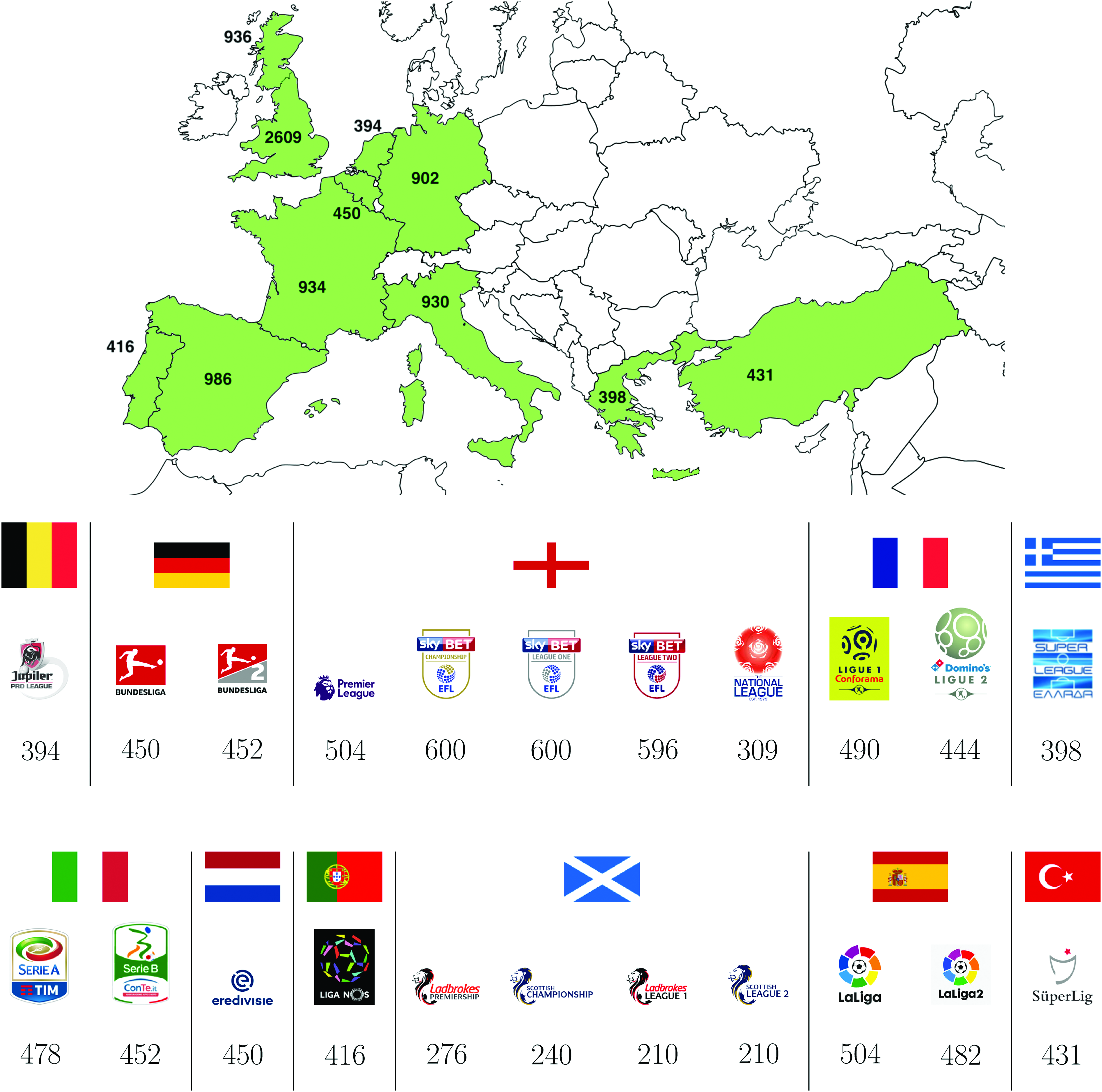
Data were extracted from the Football-Data repository,⁸¹ and they include the results of all matches for 513 European national championships over the 25-year range 1993/94–2017/18. In detail, data for 22 divisions of 11 countries at five different levels are studied, giving a total of 9386 series for 746 unique teams. Championships grouped by league and country are shown in Figure 1.

FIG. 1.

Distribution of the 9386 time series in the database by nation and division. Color images are available online.

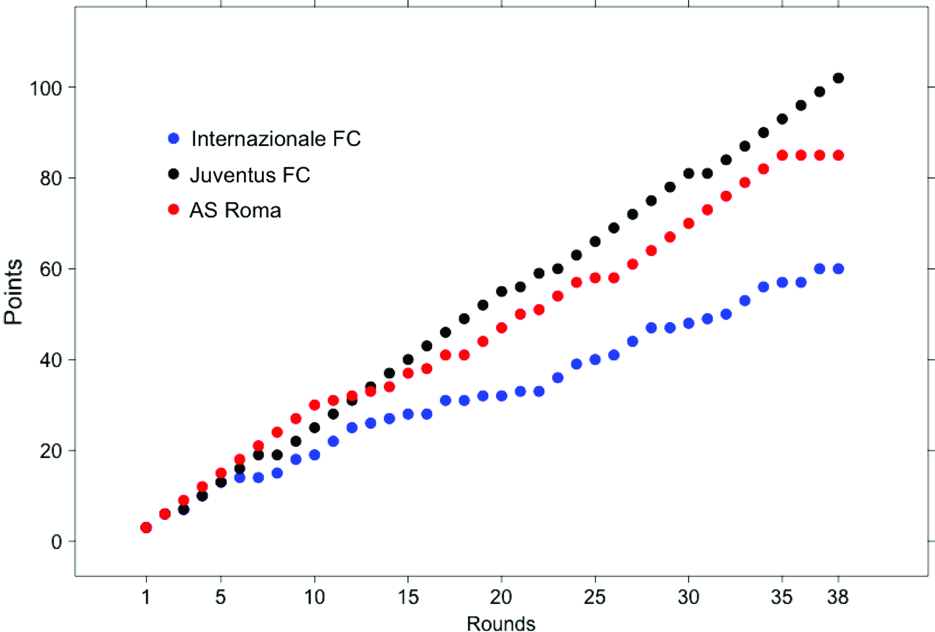
For our purposes, all 9386 time series are described by the independent variable rounds and by the dependent variable points, keeping track of the accumulated points gained by a team during the rounds of a season-long campaign, as shown in Figure 2.

FIG. 2.

Time series of the points earned by Juventus FC (black), AS Roma (red), and Internazionale FC (blue) during the 2014/15 Serie A campaign. The x-axis shows the 38 matchdays, and the y-axis shows the accumulated points. Color images are available online.

Methods

All models were computed in the R environment⁸² using the packages stats for linear/quadratic/cubic and stats for the ARIMA and the exponential smoothing state space (ETS) models. Confidence intervals were computed via the Student's bootstrap procedure^83,84 using the version described in Davison and Hinkley⁸⁵ and implemented in the boot.ci function of the boot R package.

In detail, let T be a team participating in a league whose season consists of n rounds, and let T_i be the number of points earned by T after the ith round, so that T_n is the total number of points at the end of season. Let t_s be an integer between 1 and \documentclass{aastex}\usepackage{amsbsy}\usepackage{amsfonts}\usepackage{amssymb}\usepackage{bm}\usepackage{mathrsfs}\usepackage{pifont}\usepackage{stmaryrd}\usepackage{textcomp}\usepackage{portland, xspace}\usepackage{amsmath, amsxtra}\usepackage{upgreek}\pagestyle{empty}\DeclareMathSizes{10}{9}{7}{6}\begin{document} $$n - 1$$ \end{document} , and let \documentclass{aastex}\usepackage{amsbsy}\usepackage{amsfonts}\usepackage{amssymb}\usepackage{bm}\usepackage{mathrsfs}\usepackage{pifont}\usepackage{stmaryrd}\usepackage{textcomp}\usepackage{portland, xspace}\usepackage{amsmath, amsxtra}\usepackage{upgreek}\pagestyle{empty}\DeclareMathSizes{10}{9}{7}{6}\begin{document} $$L_T^{{t_s}}$$ \end{document} be a model trained on \documentclass{aastex}\usepackage{amsbsy}\usepackage{amsfonts}\usepackage{amssymb}\usepackage{bm}\usepackage{mathrsfs}\usepackage{pifont}\usepackage{stmaryrd}\usepackage{textcomp}\usepackage{portland, xspace}\usepackage{amsmath, amsxtra}\usepackage{upgreek}\pagestyle{empty}\DeclareMathSizes{10}{9}{7}{6}\begin{document} $$( 1 , {T_1} ) , \ldots , ( n - {t_s} , {T_{n - {t_s}}} )$$ \end{document} . Define \documentclass{aastex}\usepackage{amsbsy}\usepackage{amsfonts}\usepackage{amssymb}\usepackage{bm}\usepackage{mathrsfs}\usepackage{pifont}\usepackage{stmaryrd}\usepackage{textcomp}\usepackage{portland, xspace}\usepackage{amsmath, amsxtra}\usepackage{upgreek}\pagestyle{empty}\DeclareMathSizes{10}{9}{7}{6}\begin{document} $$ { \bar { T}_n} = \lfloor L_T^{{t_s}} ( n ) \rfloor$$ \end{document} as the estimated number of total points earned by T as the largest integer smaller than the extrapolation of \documentclass{aastex}\usepackage{amsbsy}\usepackage{amsfonts}\usepackage{amssymb}\usepackage{bm}\usepackage{mathrsfs}\usepackage{pifont}\usepackage{stmaryrd}\usepackage{textcomp}\usepackage{portland, xspace}\usepackage{amsmath, amsxtra}\usepackage{upgreek}\pagestyle{empty}\DeclareMathSizes{10}{9}{7}{6}\begin{document} $$L_T^{{t_s}}$$ \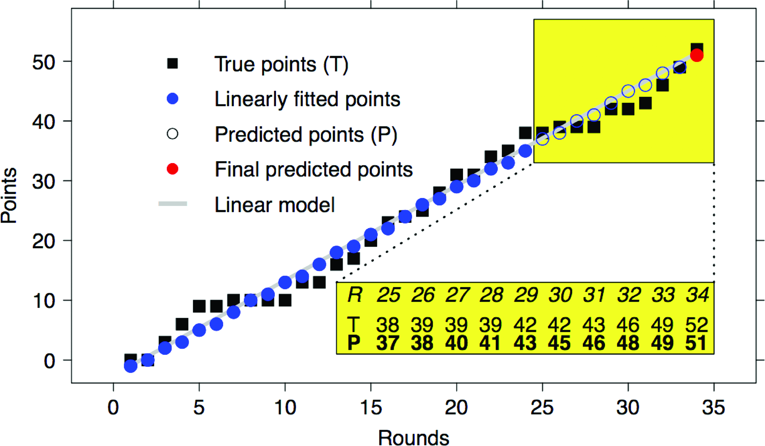end{document} computed on the point n. In Figure 3, an example is shown of the linear modeling of Schalke 04 season in the Bundesliga 2013/14, where the final number of earned points is predicted for \documentclass{aastex}\usepackage{amsbsy}\usepackage{amsfonts}\usepackage{amssymb}\usepackage{bm}\usepackage{mathrsfs}\usepackage{pifont}\usepackage{stmaryrd}\usepackage{textcomp}\usepackage{portland, xspace}\usepackage{amsmath, amsxtra}\usepackage{upgreek}\pagestyle{empty}\DeclareMathSizes{10}{9}{7}{6}\begin{document} $${t_s} = 10$$ \end{document} .

FIG. 3.

Points earned by Schalke 04 in the Bundesliga 2013/14 season (T, black square) and their approximation (circles) through a linear model (gray line) trained on the first 24 rounds (blue filled circles) and extrapolated on the last 10 rounds (P, white and red circles), highlighted in the yellow box. In the bottom-right yellow table, the comparison between the real points (T) and the predicted points (P) on the last 10 rounds. Color images are available online.

Finally, quantitative comparison between tournament standings (predicted and actual) is computed by mean of Spearman's rank correlation coefficient ρ⁸⁶ and by the total absolute displacement d,⁸⁷ defined as the normalized sum of the differences between rankings (see Appendix A for mathematical details and examples on the metric d).

Results

In what follows, we will estimate the total number of points earned by a team by mean of a linear model trained on the first \documentclass{aastex}\usepackage{amsbsy}\usepackage{amsfonts}\usepackage{amssymb}\usepackage{bm}\usepackage{mathrsfs}\usepackage{pifont}\usepackage{stmaryrd}\usepackage{textcomp}\usepackage{portland, xspace}\usepackage{amsmath, amsxtra}\usepackage{upgreek}\pagestyle{empty}\DeclareMathSizes{10}{9}{7}{6}\begin{document} $$n - {t_s}$$ \end{document} matches of the seasons, for several values of t_s, for n the total number of matches in the season. Furthermore, we will derive, for each championship, the estimated final league table to be compared to the actual standing.

Simulations

As a synthetic benchmark, \documentclass{aastex}\usepackage{amsbsy}\usepackage{amsfonts}\usepackage{amssymb}\usepackage{bm}\usepackage{mathrsfs}\usepackage{pifont}\usepackage{stmaryrd}\usepackage{textcomp}\usepackage{portland, xspace}\usepackage{amsmath, amsxtra}\usepackage{upgreek}\pagestyle{empty}\DeclareMathSizes{10}{9}{7}{6}\begin{document} $${10^4}$$ \end{document} series are randomly generated with \documentclass{aastex}\usepackage{amsbsy}\usepackage{amsfonts}\usepackage{amssymb}\usepackage{bm}\usepackage{mathrsfs}\usepackage{pifont}\usepackage{stmaryrd}\usepackage{textcomp}\usepackage{portland, xspace}\usepackage{amsmath, amsxtra}\usepackage{upgreek}\pagestyle{empty}\DeclareMathSizes{10}{9}{7}{6}\begin{document} $$n = 38$$ \end{document} , \documentclass{aastex}\usepackage{amsbsy}\usepackage{amsfonts}\usepackage{amssymb}\usepackage{bm}\usepackage{mathrsfs}\usepackage{pifont}\usepackage{stmaryrd}\usepackage{textcomp}\usepackage{portland, xspace}\usepackage{amsmath, amsxtra}\usepackage{upgreek}\pagestyle{empty}\DeclareMathSizes{10}{9}{7}{6}\begin{document} $${T_i} = {T_{i - 1}} + \xi$$ \end{document} with \documentclass{aastex}\usepackage{amsbsy}\usepackage{amsfonts}\usepackage{amssymb}\usepackage{bm}\usepackage{mathrsfs}\usepackage{pifont}\usepackage{stmaryrd}\usepackage{textcomp}\usepackage{portland, xspace}\usepackage{amsmath, amsxtra}\usepackage{upgreek}\pagestyle{empty}\DeclareMathSizes{10}{9}{7}{6}\begin{document} $${T_0} = 0$$ \end{document} , and \documentclass{aastex}\usepackage{amsbsy}\usepackage{amsfonts}\usepackage{amssymb}\usepackage{bm}\usepackage{mathrsfs}\usepackage{pifont}\usepackage{stmaryrd}\usepackage{textcomp}\usepackage{portland, xspace}\usepackage{amsmath, amsxtra}\usepackage{upgreek}\pagestyle{empty}\DeclareMathSizes{10}{9}{7}{6}\begin{document} $$\xi$$ \end{document} equal to 0, 1, or 3 with a probability of 1/3. Then \documentclass{aastex}\usepackage{amsbsy}\usepackage{amsfonts}\usepackage{amssymb}\usepackage{bm}\usepackage{mathrsfs}\usepackage{pifont}\usepackage{stmaryrd}\usepackage{textcomp}\usepackage{portland, xspace}\usepackage{amsmath, amsxtra}\usepackage{upgreek}\pagestyle{empty}\DeclareMathSizes{10}{9}{7}{6}\begin{document} $${ \bar { T}_n} = \lfloor L_T^{{t_s}} ( n ) \rfloor$$ \end{document} is computed together with CI for L the linear, the quadratic, the cubic, the ARIMA, or the ETS model, for \documentclass{aastex}\usepackage{amsbsy}\usepackage{amsfonts}\usepackage{amssymb}\usepackage{bm}\usepackage{mathrsfs}\usepackage{pifont}\usepackage{stmaryrd}\usepackage{textcomp}\usepackage{portland, xspace}\usepackage{amsmath, amsxtra}\usepackage{upgreek}\pagestyle{empty}\DeclareMathSizes{10}{9}{7}{6}\begin{document} $${t_s} = 1 , \ldots , 19$$ \end{document} . Both the ARIMA and the ETS models are automatically optimized by the default R call, and the results are reported in Table 1. The ARIMA model is consistently the best, but the linear model represents a solid and simpler alternative not needing any optimization, while the quadratic and the cubic models have poor performances, especially when the training set becomes smaller: when estimating the final number of points using the first 28 rounds (out of 38), the linear, ARIMA, and ETS models show an average error of 4 points, while the quadratic and the cubic models have an error of 7 and 14 points, respectively. Thus, the linear trend is a good approximation of the null model with random results. The critical feature that supports the fair performance of the linear model in the longitudinal data of teams' yearly campaings is the fact that the successive increments \documentclass{aastex}\usepackage{amsbsy}\usepackage{amsfonts}\usepackage{amssymb}\usepackage{bm}\usepackage{mathrsfs}\usepackage{pifont}\usepackage{stmaryrd}\usepackage{textcomp}\usepackage{portland, xspace}\usepackage{amsmath, amsxtra}\usepackage{upgreek}\pagestyle{empty}\DeclareMathSizes{10}{9}{7}{6}\begin{document} $$\xi$$ \end{document} are non-negative and small. In fact, allowing \documentclass{aastex}\usepackage{amsbsy}\usepackage{amsfonts}\usepackage{amssymb}\usepackage{bm}\usepackage{mathrsfs}\usepackage{pifont}\usepackage{stmaryrd}\usepackage{textcomp}\usepackage{portland, xspace}\usepackage{amsmath, amsxtra}\usepackage{upgreek}\pagestyle{empty}\DeclareMathSizes{10}{9}{7}{6}\begin{document} $$\xi$$ \end{document} to take larger values quickly worsens the fit of the linear model, as shown from the three examples reported in Table 2. The above experiment was replicated with different sets of values for \documentclass{aastex}\usepackage{amsbsy}\usepackage{amsfonts}\usepackage{amssymb}\usepackage{bm}\usepackage{mathrsfs}\usepackage{pifont}\usepackage{stmaryrd}\usepackage{textcomp}\usepackage{portland, xspace}\usepackage{amsmath, amsxtra}\usepackage{upgreek}\pagestyle{empty}\DeclareMathSizes{10}{9}{7}{6}\begin{document} $$\xi$$ \end{document} , namely \documentclass{aastex}\usepackage{amsbsy}\usepackage{amsfonts}\usepackage{amssymb}\usepackage{bm}\usepackage{mathrsfs}\usepackage{pifont}\usepackage{stmaryrd}\usepackage{textcomp}\usepackage{portland, xspace}\usepackage{amsmath, amsxtra}\usepackage{upgreek}\pagestyle{empty}\DeclareMathSizes{10}{9}{7}{6}\begin{document} $$\{ 0 , 1 , 6 \} $$ \end{document} , \documentclass{aastex}\usepackage{amsbsy}\usepackage{amsfonts}\usepackage{amssymb}\usepackage{bm}\usepackage{mathrsfs}\usepackage{pifont}\usepackage{stmaryrd}\usepackage{textcomp}\usepackage{portland, xspace}\usepackage{amsmath, amsxtra}\usepackage{upgreek}\pagestyle{empty}\DeclareMathSizes{10}{9}{7}{6}\begin{document} $$\{ 0 , 1 , 3 , 6 \} $$ \end{document} , and \documentclass{aastex}\usepackage{amsbsy}\usepackage{amsfonts}\usepackage{amssymb}\usepackage{bm}\usepackage{mathrsfs}\usepackage{pifont}\usepackage{stmaryrd}\usepackage{textcomp}\usepackage{portland, xspace}\usepackage{amsmath, amsxtra}\usepackage{upgreek}\pagestyle{empty}\DeclareMathSizes{10}{9}{7}{6}\begin{document} $$\{ 0 , 1 , 2 , 3 , 4 , 5 \} $$ \end{document} , and in all threee cases the average error of the linear model was larger than the one resulting from the true setting \documentclass{aastex}\usepackage{amsbsy}\usepackage{amsfonts}\usepackage{amssymb}\usepackage{bm}\usepackage{mathrsfs}\usepackage{pifont}\usepackage{stmaryrd}\usepackage{textcomp}\usepackage{portland, xspace}\usepackage{amsmath, amsxtra}\usepackage{upgreek}\pagestyle{empty}\DeclareMathSizes{10}{9}{7}{6}\begin{document} $$\{ 0 , 1 , 3 \} $$ \end{document} .

Table 1.

Prediction error of the linear (L), quadratic (Q), cubic (C), ARIMA (A), and ETS (E) models on 10⁴ simulated time series on n = 38 rounds

n – t_s	Ll	Lm	Lu	Ql	Qm	Qu	Cl	Cm	Cu
19	6.76	6.85	6.95	18.94	19.21	19.48	74.54	75.50	76.60
20	6.38	6.47	6.57	17.02	17.30	17.54	60.78	61.71	62.53
21	5.99	6.08	6.18	15.04	15.28	15.50	50.08	50.81	51.52
22	5.83	5.92	6.01	13.36	13.54	13.73	41.95	42.58	43.22
23	5.56	5.64	5.72	12.09	12.26	12.45	35.01	35.54	36.05
24	5.27	5.35	5.43	10.75	10.91	11.07	28.89	29.31	29.74
25	4.99	5.06	5.14	9.56	9.70	9.85	23.84	24.19	24.58
26	4.71	4.78	4.85	8.60	8.73	8.86	20.17	20.45	20.78
27	4.54	4.60	4.67	7.63	7.73	7.84	16.80	17.06	17.30
28	4.29	4.35	4.42	6.92	7.02	7.11	13.78	13.98	14.19
29	4.09	4.15	4.21	6.15	6.23	6.33	11.44	11.60	11.78
30	3.85	3.90	3.97	5.54	5.62	5.70	9.47	9.62	9.76
31	3.67	3.73	3.79	4.83	4.90	4.98	7.91	8.02	8.14
32	3.39	3.44	3.49	4.35	4.41	4.47	6.51	6.61	6.71
33	3.18	3.23	3.28	3.80	3.86	3.92	5.26	5.34	5.42
34	3.00	3.04	3.09	3.29	3.34	3.39	4.24	4.30	4.37
35	2.76	2.80	2.84	2.83	2.87	2.91	3.35	3.40	3.44
36	2.56	2.60	2.64	2.41	2.44	2.48	2.56	2.60	2.64
37	2.33	2.37	2.40	1.99	2.02	2.04	1.89	1.92	1.95

n – t_s	El	Em	Eu	Al	Am	Au
19	8.34	8.48	8.62	6.80	6.91	7.03
20	7.91	8.03	8.16	6.20	6.30	6.40
21	7.23	7.34	7.47	5.83	5.92	6.01
22	6.79	6.90	7.01	5.53	5.62	5.70
23	6.43	6.54	6.64	5.26	5.35	5.43
24	5.98	6.08	6.18	5.00	5.07	5.15
25	5.48	5.57	5.66	4.64	4.71	4.78
26	5.11	5.20	5.29	4.31	4.37	4.45
27	4.77	4.84	4.92	4.08	4.14	4.21
28	4.41	4.48	4.55	3.81	3.86	3.92
29	4.00	4.06	4.13	3.55	3.60	3.66
30	3.71	3.76	3.82	3.28	3.33	3.38
31	3.33	3.38	3.43	3.02	3.06	3.11
32	3.00	3.04	3.09	2.76	2.80	2.84
33	2.60	2.64	2.69	2.43	2.46	2.50
34	2.29	2.32	2.35	2.15	2.18	2.21
35	1.91	1.94	1.97	1.82	1.85	1.88
36	1.54	1.56	1.59	1.49	1.51	1.53
37	1.10	1.11	1.13	1.08	1.09	1.11

For each model, the mean error (m) and the lower (l) and upper (l) Student's bootstrap confidence intervals (CIs) are reported.

ARIMA, autoregressive integrated moving average; ETS, exponential smoothing state space.

Table 2.

Prediction error of the linear model on 10⁴ simulated time series on n = 38 rounds for different sets of values of ξ

	ξ ∈{0,1,6}			ξ ∈{0,3,6}			ξ ∈{0,1,2,3,4,5}
n – t_s	l	m	u	l	m	u	l	m	u
19	14.06	14.25	14.47	12.25	12.44	12.62	9.21	9.36	9.50
20	13.41	13.60	13.82	11.75	11.93	12.12	8.80	8.94	9.06
21	12.85	13.04	13.23	11.05	11.21	11.37	8.29	8.42	8.55
22	12.03	12.19	12.37	10.52	10.67	10.83	8.01	8.13	8.25
23	11.56	11.74	11.91	10.09	10.23	10.38	7.59	7.70	7.81
24	11.04	11.19	11.36	9.69	9.83	9.97	7.21	7.32	7.43
25	10.65	10.80	10.97	9.20	9.34	9.47	6.80	6.90	7.02
26	10.08	10.22	10.38	8.71	8.84	8.98	6.42	6.51	6.60
27	9.57	9.70	9.86	8.29	8.41	8.53	6.17	6.26	6.35
28	8.95	9.09	9.23	7.86	7.97	8.08	5.82	5.91	6.00
29	8.46	8.59	8.73	7.53	7.64	7.75	5.55	5.63	5.71
30	8.14	8.27	8.39	7.18	7.28	7.38	5.31	5.39	5.47
31	7.62	7.75	7.86	6.70	6.81	6.90	4.94	5.01	5.09
32	7.24	7.34	7.45	6.27	6.36	6.44	4.63	4.70	4.77
33	6.73	6.84	6.96	5.91	6.00	6.09	4.38	4.45	4.52
34	6.31	6.40	6.49	5.48	5.56	5.64	4.11	4.18	4.24
35	5.79	5.87	5.95	5.09	5.17	5.24	3.78	3.84	3.90
36	5.34	5.42	5.50	4.66	4.73	4.80	3.51	3.56	3.61
37	4.89	4.96	5.03	4.24	4.30	4.37	3.16	3.20	3.25

For each model the mean error (m) and the lower (l) and upper (l) Student's bootstrap CIs are reported.

Team performance prediction

For the 9386 seasonal time series T, we estimate \documentclass{aastex}\usepackage{amsbsy}\usepackage{amsfonts}\usepackage{amssymb}\usepackage{bm}\usepackage{mathrsfs}\usepackage{pifont}\usepackage{stmaryrd}\usepackage{textcomp}\usepackage{portland, xspace}\usepackage{amsmath, amsxtra}\usepackage{upgreek}\pagestyle{empty}\DeclareMathSizes{10}{9}{7}{6}\begin{document} $${ \bar { T}_n}$$ \end{document} for \documentclass{aastex}\usepackage{amsbsy}\usepackage{amsfonts}\usepackage{amssymb}\usepackage{bm}\usepackage{mathrsfs}\usepackage{pifont}\usepackage{stmaryrd}\usepackage{textcomp}\usepackage{portland, xspace}\usepackage{amsmath, amsxtra}\usepackage{upgreek}\pagestyle{empty}\DeclareMathSizes{10}{9}{7}{6}\begin{document} $${t_s} = 1 , \ldots , 20$$ \end{document} , with linear, quadratic, cubic, ARIMA, and ETS models. As a comparative baseline, we also interpolate \documentclass{aastex}\usepackage{amsbsy}\usepackage{amsfonts}\usepackage{amssymb}\usepackage{bm}\usepackage{mathrsfs}\usepackage{pifont}\usepackage{stmaryrd}\usepackage{textcomp}\usepackage{portland, xspace}\usepackage{amsmath, amsxtra}\usepackage{upgreek}\pagestyle{empty}\DeclareMathSizes{10}{9}{7}{6}\begin{document} $${ \bar { T}_n}$$ \end{document} as \documentclass{aastex}\usepackage{amsbsy}\usepackage{amsfonts}\usepackage{amssymb}\usepackage{bm}\usepackage{mathrsfs}\usepackage{pifont}\usepackage{stmaryrd}\usepackage{textcomp}\usepackage{portland, xspace}\usepackage{amsmath, amsxtra}\usepackage{upgreek}\pagestyle{empty}\DeclareMathSizes{10}{9}{7}{6}\begin{document} $$ { T_ { n - s } } \cdot \frac { n } { { n - s } } $$ \end{document} . In Table 3, we list the mean and the confidence intervals for \documentclass{aastex}\usepackage{amsbsy}\usepackage{amsfonts}\usepackage{amssymb}\usepackage{bm}\usepackage{mathrsfs}\usepackage{pifont}\usepackage{stmaryrd}\usepackage{textcomp}\usepackage{portland, xspace}\usepackage{amsmath, amsxtra}\usepackage{upgreek}\pagestyle{empty}\DeclareMathSizes{10}{9}{7}{6}\begin{document} $$\vert { \bar { T}_n} - {T_n} \vert$$ \end{document} for the five models.

Table 3.

Mean and bootstrap CIs of \documentclass{aastex}\usepackage{amsbsy}\usepackage{amsfonts}\usepackage{amssymb}\usepackage{bm}\usepackage{mathrsfs}\usepackage{pifont}\usepackage{stmaryrd}\usepackage{textcomp}\usepackage{portland, xspace}\usepackage{amsmath, amsxtra}\usepackage{upgreek}\pagestyle{empty}\DeclareMathSizes{10}{9}{7}{6}\begin{document} $$\vert { \bar {{T}}_{{n}}} - {{{T_n}}} \vert$$ \end{document} for the linear, quadratic, cubic, ARIMA, and ETS models and the interpolation baseline

Model	Lower CI	\documentclass{aastex}\usepackage{amsbsy}\usepackage{amsfonts}\usepackage{amssymb}\usepackage{bm}\usepackage{mathrsfs}\usepackage{pifont}\usepackage{stmaryrd}\usepackage{textcomp}\usepackage{portland, xspace}\usepackage{amsmath, amsxtra}\usepackage{upgreek}\pagestyle{empty}\DeclareMathSizes{10}{9}{7}{6}\begin{document} $$\overline { \vert {{ \bar {T}}_{ n} - {T_n} \vert}}$$ \end{document}	Upper CI
Linear	4.55	4.57	4.59
Quadratic	8.15	8.19	8.23
Cubic	22.10	22.25	22.40
ARIMA	3.99	4.01	4.03
ETS	4.82	4.85	4.87
Baseline	13.29	13.37	13.45

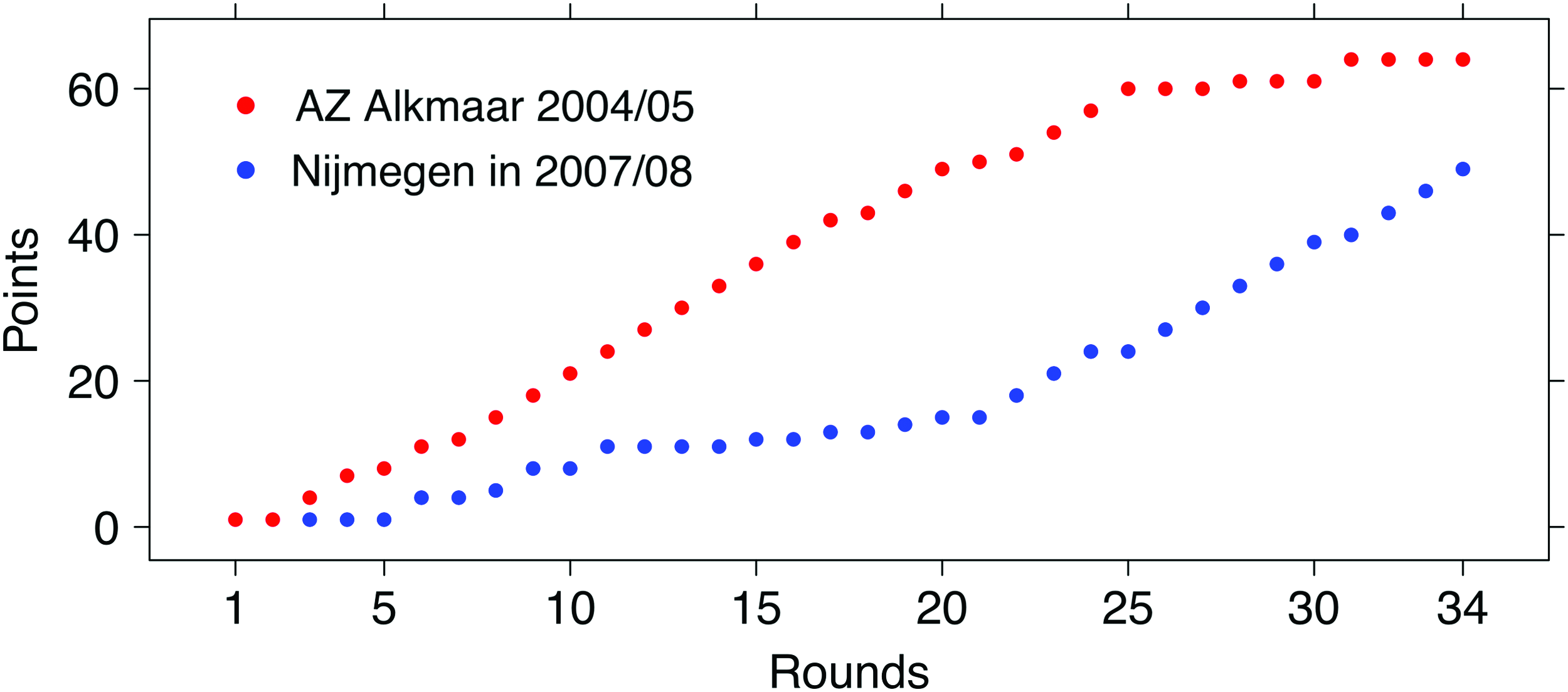
Results for the six models are all mutually statistically different, with p-values <10⁻¹⁶. While quadratic and cubic models have very poor predictivity (with the cubic model performing even worse than the interpolation baseline), linear, ETS, and ARIMA models produce similar and better results, supporting the claim of an overall linear trend in points evolution. These results imply that overall, the seasonal trend is not linear, since the nonlinear ARIMA model fits better (and Pearson's correlation between the ARIMA and linear models is 0.76), but the simpler linear model represents a valid approximation. In Figure 4, we show two cases (both in Dutch Eredivisie) where the nonlinearity instead is particularly evident, namely AZ Alkmaar in 2004/05 and Nijmegen in 2007/08. In both cases, the trend for the last part of the season is very different from the initial part.

FIG. 4.

Points earned by AZ Alkmaar in the Eredivisie 2004/05 season (red) and by Nijmegen in the 2007/08 season (blue). In both cases, there is a remarkably different trend between the initial and the final part of the season, making both dynamics nonlinear. Color images are available online.

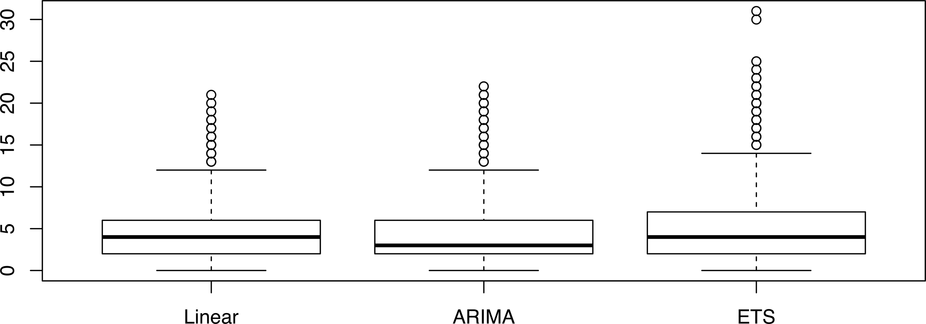
In what follows, as a representative case, we set \documentclass{aastex}\usepackage{amsbsy}\usepackage{amsfonts}\usepackage{amssymb}\usepackage{bm}\usepackage{mathrsfs}\usepackage{pifont}\usepackage{stmaryrd}\usepackage{textcomp}\usepackage{portland, xspace}\usepackage{amsmath, amsxtra}\usepackage{upgreek}\pagestyle{empty}\DeclareMathSizes{10}{9}{7}{6}\begin{document} $${t_s} = 10$$ \end{document} , that is, for each series, we use all the rounds except for the last 10 as the training set, and we predict the final figure of earned points. Overall, when \documentclass{aastex}\usepackage{amsbsy}\usepackage{amsfonts}\usepackage{amssymb}\usepackage{bm}\usepackage{mathrsfs}\usepackage{pifont}\usepackage{stmaryrd}\usepackage{textcomp}\usepackage{portland, xspace}\usepackage{amsmath, amsxtra}\usepackage{upgreek}\pagestyle{empty}\DeclareMathSizes{10}{9}{7}{6}\begin{document} $${t_s} = 10$$ \end{document} , the average prediction error of the final number of points is 4.43 for the linear model, 3.93 for the ARIMA model, and 4.62 for the ETS model, but the boxplots for the three models almost overlap, as shown in Figure 5. In this case, the average prediction error for the interpolation baseline model is 14.24, with a confidence interval of 14.07–14.40. Consistency of the results with those obtained in the general situation indicates that choosing \documentclass{aastex}\usepackage{amsbsy}\usepackage{amsfonts}\usepackage{amssymb}\usepackage{bm}\usepackage{mathrsfs}\usepackage{pifont}\usepackage{stmaryrd}\usepackage{textcomp}\usepackage{portland, xspace}\usepackage{amsmath, amsxtra}\usepackage{upgreek}\pagestyle{empty}\DeclareMathSizes{10}{9}{7}{6}\begin{document} $${t_s} = 10$$ \end{document} as the representative case is a meaningful choice (the full linear prediction results for all teams, leagues, and seasons can be found in the Supplementary Data).

FIG. 5.

Box and whisker plot of the distribution of absolute value of the prediction errors, for t_s = 10, for the whole set of 9386 time series, by the linear, autoregressive integrated moving average, and exponential smoothing state space model.

We also add here the comparison with algorithms from a well-known family of algorithms, variants of the original Pythagorean Expectation (PE) method, originally developed for baseball in James,⁸⁰ recently adapted for football by Hamilton ⁷⁹ and then further optimized by several authors.^88–91 The basic PE model has the form \documentclass{aastex}\usepackage{amsbsy}\usepackage{amsfonts}\usepackage{amssymb}\usepackage{bm}\usepackage{mathrsfs}\usepackage{pifont}\usepackage{stmaryrd}\usepackage{textcomp}\usepackage{portland, xspace}\usepackage{amsmath, amsxtra}\usepackage{upgreek}\pagestyle{empty}\DeclareMathSizes{10}{9}{7}{6}\begin{document} \begin{align*} \rm { earned \;points = { \frac { G { F^ { { \gamma _1 } } } } { G { F^ { { \gamma _2 } } } + G { A^ { { \gamma _3 } } } } } \cdot \lambda \cdot \# rounds } \; , \end{align*} \end{document}

and thus is different from the other model, since it is not a model for the dynamics of the time series of gained points. In the original article,⁷⁹ \documentclass{aastex}\usepackage{amsbsy}\usepackage{amsfonts}\usepackage{amssymb}\usepackage{bm}\usepackage{mathrsfs}\usepackage{pifont}\usepackage{stmaryrd}\usepackage{textcomp}\usepackage{portland, xspace}\usepackage{amsmath, amsxtra}\usepackage{upgreek}\pagestyle{empty}\DeclareMathSizes{10}{9}{7}{6}\begin{document} $${ \gamma _1} = { \gamma _2} = { \gamma _3}$$ \end{document} were estimated on the available data by a Weibull distribution and \documentclass{aastex}\usepackage{amsbsy}\usepackage{amsfonts}\usepackage{amssymb}\usepackage{bm}\usepackage{mathrsfs}\usepackage{pifont}\usepackage{stmaryrd}\usepackage{textcomp}\usepackage{portland, xspace}\usepackage{amsmath, amsxtra}\usepackage{upgreek}\pagestyle{empty}\DeclareMathSizes{10}{9}{7}{6}\begin{document} $$\lambda = 1$$ \end{document} , while the following variants have different values for the three \documentclass{aastex}\usepackage{amsbsy}\usepackage{amsfonts}\usepackage{amssymb}\usepackage{bm}\usepackage{mathrsfs}\usepackage{pifont}\usepackage{stmaryrd}\usepackage{textcomp}\usepackage{portland, xspace}\usepackage{amsmath, amsxtra}\usepackage{upgreek}\pagestyle{empty}\DeclareMathSizes{10}{9}{7}{6}\begin{document} $$\gamma$$ \end{document} parameters and \documentclass{aastex}\usepackage{amsbsy}\usepackage{amsfonts}\usepackage{amssymb}\usepackage{bm}\usepackage{mathrsfs}\usepackage{pifont}\usepackage{stmaryrd}\usepackage{textcomp}\usepackage{portland, xspace}\usepackage{amsmath, amsxtra}\usepackage{upgreek}\pagestyle{empty}\DeclareMathSizes{10}{9}{7}{6}\begin{document} $$\lambda$$ \end{document} is >1 to account for ties and 3-point wins. In what follows, we tried several different sets of parameters, and we report the results for the best performing values \documentclass{aastex}\usepackage{amsbsy}\usepackage{amsfonts}\usepackage{amssymb}\usepackage{bm}\usepackage{mathrsfs}\usepackage{pifont}\usepackage{stmaryrd}\usepackage{textcomp}\usepackage{portland, xspace}\usepackage{amsmath, amsxtra}\usepackage{upgreek}\pagestyle{empty}\DeclareMathSizes{10}{9}{7}{6}\begin{document} $${ \gamma _1} = 1.5$$ \end{document} , \documentclass{aastex}\usepackage{amsbsy}\usepackage{amsfonts}\usepackage{amssymb}\usepackage{bm}\usepackage{mathrsfs}\usepackage{pifont}\usepackage{stmaryrd}\usepackage{textcomp}\usepackage{portland, xspace}\usepackage{amsmath, amsxtra}\usepackage{upgreek}\pagestyle{empty}\DeclareMathSizes{10}{9}{7}{6}\begin{document} $${ \gamma _2} = 1.08$$ \end{document} , \documentclass{aastex}\usepackage{amsbsy}\usepackage{amsfonts}\usepackage{amssymb}\usepackage{bm}\usepackage{mathrsfs}\usepackage{pifont}\usepackage{stmaryrd}\usepackage{textcomp}\usepackage{portland, xspace}\usepackage{amsmath, amsxtra}\usepackage{upgreek}\pagestyle{empty}\DeclareMathSizes{10}{9}{7}{6}\begin{document} $${ \gamma _3} = 1.13$$ \end{document} , and \documentclass{aastex}\usepackage{amsbsy}\usepackage{amsfonts}\usepackage{amssymb}\usepackage{bm}\usepackage{mathrsfs}\usepackage{pifont}\usepackage{stmaryrd}\usepackage{textcomp}\usepackage{portland, xspace}\usepackage{amsmath, amsxtra}\usepackage{upgreek}\pagestyle{empty}\DeclareMathSizes{10}{9}{7}{6}\begin{document} $$\lambda = 2.31$$ \end{document} . Although all these models are known to achieve reasonably good diagnostic results across different leagues and seasons in modeling the team's points, they do not perform similarly well in prediction: for \documentclass{aastex}\usepackage{amsbsy}\usepackage{amsfonts}\usepackage{amssymb}\usepackage{bm}\usepackage{mathrsfs}\usepackage{pifont}\usepackage{stmaryrd}\usepackage{textcomp}\usepackage{portland, xspace}\usepackage{amsmath, amsxtra}\usepackage{upgreek}\pagestyle{empty}\DeclareMathSizes{10}{9}{7}{6}\begin{document} $${t_s} = 10$$ \end{document} , the average prediction error of the final number of points is 6.93.

Consider the (linear) predictivity ( \documentclass{aastex}\usepackage{amsbsy}\usepackage{amsfonts}\usepackage{amssymb}\usepackage{bm}\usepackage{mathrsfs}\usepackage{pifont}\usepackage{stmaryrd}\usepackage{textcomp}\usepackage{portland, xspace}\usepackage{amsmath, amsxtra}\usepackage{upgreek}\pagestyle{empty}\DeclareMathSizes{10}{9}{7}{6}\begin{document} $$\overline { \vert {{ \bar { T}}_n} - {T_n} \vert }$$ \end{document} for \documentclass{aastex}\usepackage{amsbsy}\usepackage{amsfonts}\usepackage{amssymb}\usepackage{bm}\usepackage{mathrsfs}\usepackage{pifont}\usepackage{stmaryrd}\usepackage{textcomp}\usepackage{portland, xspace}\usepackage{amsmath, amsxtra}\usepackage{upgreek}\pagestyle{empty}\DeclareMathSizes{10}{9}{7}{6}\begin{document} $${t_s} = 10$$ \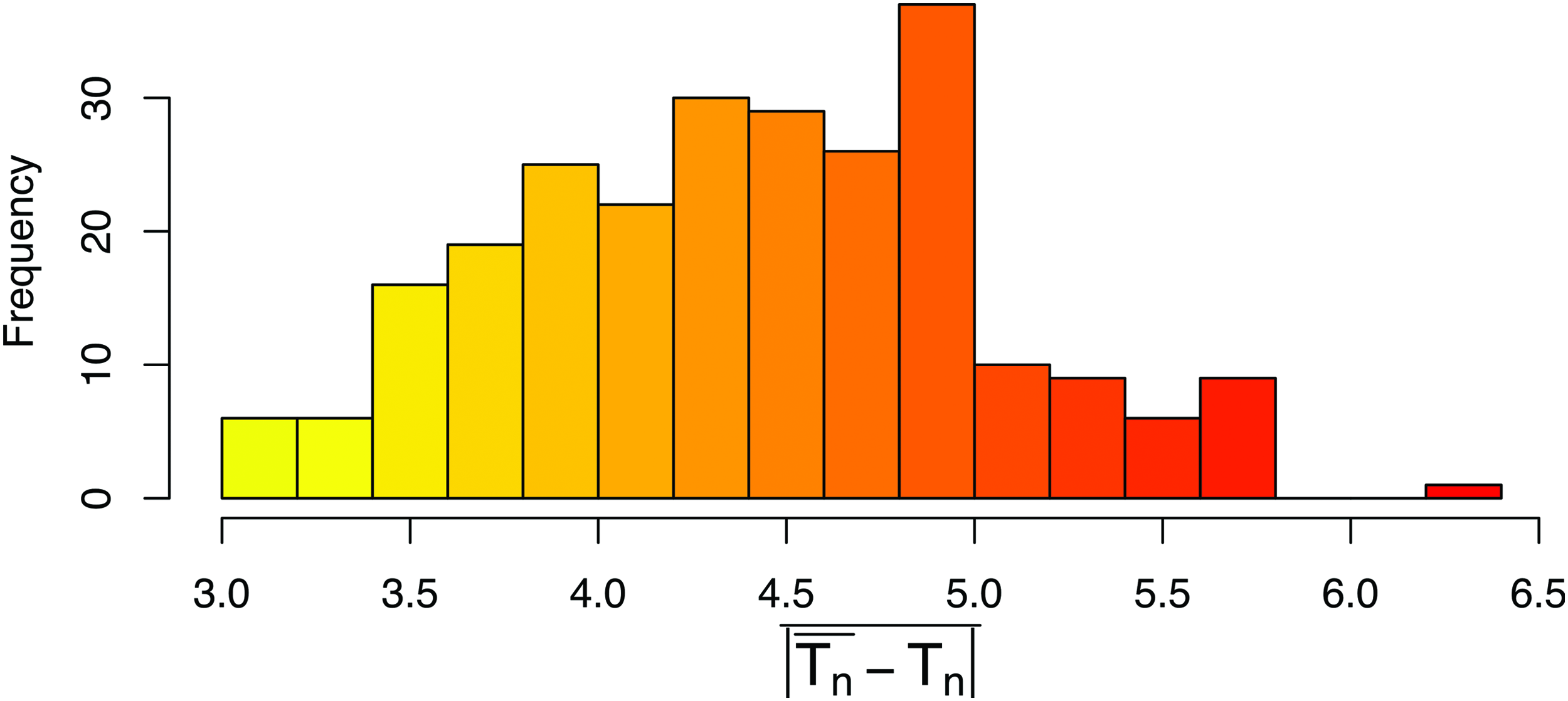end{document} ) of the set S of 258 teams that are present for ≥20/25 seasons in the available data. Figure 6 shows the histogram of the average differences between prediction and actual values. The set of values \documentclass{aastex}\usepackage{amsbsy}\usepackage{amsfonts}\usepackage{amssymb}\usepackage{bm}\usepackage{mathrsfs}\usepackage{pifont}\usepackage{stmaryrd}\usepackage{textcomp}\usepackage{portland, xspace}\usepackage{amsmath, amsxtra}\usepackage{upgreek}\pagestyle{empty}\DeclareMathSizes{10}{9}{7}{6}\begin{document} $$\overline { \vert {{ \bar { T}}_n} - {T_n} \vert }$$ \end{document} for S is Gaussian-like, with a range of 3.00–6.33 (min and max corresponding to Lorient and Dundee Utd., respectively) and a mean and median of approximately 4.4. Smaller values indicate more linear behavior of a team throughout all the considered seasons, while larger values mark the presence of one or more seasons where the sequence of results had a nonlinear trend. On the same task, again the PE algorithm has poorer performances, with an average error 7.39. In Table 4, the values \documentclass{aastex}\usepackage{amsbsy}\usepackage{amsfonts}\usepackage{amssymb}\usepackage{bm}\usepackage{mathrsfs}\usepackage{pifont}\usepackage{stmaryrd}\usepackage{textcomp}\usepackage{portland, xspace}\usepackage{amsmath, amsxtra}\usepackage{upgreek}\pagestyle{empty}\DeclareMathSizes{10}{9}{7}{6}\begin{document} $$\overline { \vert {{ \bar { T}}_n} - {T_n} \vert }$$ \end{document} are listed for the top10 Union of European Football Associations ranking teams (current standing at June 2018). Among a number of teams such as Bayern Munich, Juventus, and Manchester City whose linear trend is quite consistent through all the considered seasons ( \documentclass{aastex}\usepackage{amsbsy}\usepackage{amsfonts}\usepackage{amssymb}\usepackage{bm}\usepackage{mathrsfs}\usepackage{pifont}\usepackage{stmaryrd}\usepackage{textcomp}\usepackage{portland, xspace}\usepackage{amsmath, amsxtra}\usepackage{upgreek}\pagestyle{empty}\DeclareMathSizes{10}{9}{7}{6}\begin{document} $$\overline { \vert {{ \bar { T}}_n} - {T_n} \vert } < 4 )$$ \end{document} , Barcelona's case emerges. Barcelona's high value \documentclass{aastex}\usepackage{amsbsy}\usepackage{amsfonts}\usepackage{amssymb}\usepackage{bm}\usepackage{mathrsfs}\usepackage{pifont}\usepackage{stmaryrd}\usepackage{textcomp}\usepackage{portland, xspace}\usepackage{amsmath, amsxtra}\usepackage{upgreek}\pagestyle{empty}\DeclareMathSizes{10}{9}{7}{6}\begin{document} $$\overline { \vert {{ \bar { T}}_n} - {T_n} \vert } = 5.76$$ \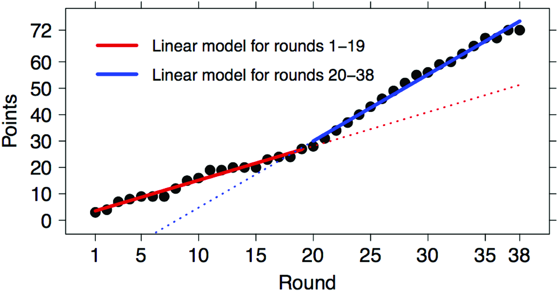end{document} is due to a number of seasons (1993/94, 2002/03, 2005/06, 2003/04, 2007/08, 2008/09, and 2010/11) where the seasonal trend was markedly nonlinear, mostly because the last matches followed a very different pattern from the initial part of the season. As an example, consider the situation in the 2003/04 campaign shown in Figure 7. The seasonal pattern is nonlinear, but it is piecewise linear, with the first and second halves of the season following two distinct linear approximations whose corresponding slopes are 1.29 and 2.52, respectively, thus in ratio almost 1:2. A similar situation happened to Juventus in the 201516 season, when they collected 12 points in the first 10 rounds, and 79 in the following 28 rounds.

FIG. 6.

Histogram of \documentclass{aastex}\usepackage{amsbsy}\usepackage{amsfonts}\usepackage{amssymb}\usepackage{bm}\usepackage{mathrsfs}\usepackage{pifont}\usepackage{stmaryrd}\usepackage{textcomp}\usepackage{portland, xspace}\usepackage{amsmath, amsxtra}\usepackage{upgreek}\pagestyle{empty}\DeclareMathSizes{10}{9}{7}{6}\begin{document} $$\overline { \vert {{ \bar T}_n} - {T_n} \vert }$$ \end{document} for the set S of 258 teams having more presences (≥20/25). Color images are available online.

FIG. 7.

Points earned by FC Barcelona (black dots) in La Liga 2003/04 and the corresponding linear models for the first (red line) and second (blue line) halves of the season. Color images are available online.

Table 4.

\documentclass{aastex}\usepackage{amsbsy}\usepackage{amsfonts}\usepackage{amssymb}\usepackage{bm}\usepackage{mathrsfs}\usepackage{pifont}\usepackage{stmaryrd}\usepackage{textcomp}\usepackage{portland, xspace}\usepackage{amsmath, amsxtra}\usepackage{upgreek}\pagestyle{empty}\DeclareMathSizes{10}{9}{7}{6}\begin{document} $$\overline { \vert {{ \bar {{T}}}_{{n}}} - {{T_n}} \vert }$$ \end{document} for the top 10 Union of European Football Associations ranking teams at November 2015 for t_s = 10

Rank	Team	\documentclass{aastex}\usepackage{amsbsy}\usepackage{amsfonts}\usepackage{amssymb}\usepackage{bm}\usepackage{mathrsfs}\usepackage{pifont}\usepackage{stmaryrd}\usepackage{textcomp}\usepackage{portland, xspace}\usepackage{amsmath, amsxtra}\usepackage{upgreek}\pagestyle{empty}\DeclareMathSizes{10}{9}{7}{6}\begin{document} $$\overline { \vert {{ \bar {T}}_{n}} - {T_n} \vert }$$ \end{document}	Rank	Team	\documentclass{aastex}\usepackage{amsbsy}\usepackage{amsfonts}\usepackage{amssymb}\usepackage{bm}\usepackage{mathrsfs}\usepackage{pifont}\usepackage{stmaryrd}\usepackage{textcomp}\usepackage{portland, xspace}\usepackage{amsmath, amsxtra}\usepackage{upgreek}\pagestyle{empty}\DeclareMathSizes{10}{9}{7}{6}\begin{document} $$\overline { \vert {{ \bar {T}}_{n}} - {T_n} \vert }$$ \end{document}
1	Real Madrid CF	4.48	6	Sevilla FC	4.24
2	Club Atlético de Madrid	5.20	7	Paris Saint-Germain	4.72
3	FC Bayern München	3.72	8	Manchester City	3.68
4	FC Barcelona	5.76	9	Arsenal FC	4.28
5	Juventus	3.72	10	Borussia Dortmund	4.84

Furthermore, differences between various countries and leagues are small for every value of t_s. As an example, for \documentclass{aastex}\usepackage{amsbsy}\usepackage{amsfonts}\usepackage{amssymb}\usepackage{bm}\usepackage{mathrsfs}\usepackage{pifont}\usepackage{stmaryrd}\usepackage{textcomp}\usepackage{portland, xspace}\usepackage{amsmath, amsxtra}\usepackage{upgreek}\pagestyle{empty}\DeclareMathSizes{10}{9}{7}{6}\begin{document} $${t_s} = 10$$ \end{document} , the value of \documentclass{aastex}\usepackage{amsbsy}\usepackage{amsfonts}\usepackage{amssymb}\usepackage{bm}\usepackage{mathrsfs}\usepackage{pifont}\usepackage{stmaryrd}\usepackage{textcomp}\usepackage{portland, xspace}\usepackage{amsmath, amsxtra}\usepackage{upgreek}\pagestyle{empty}\DeclareMathSizes{10}{9}{7}{6}\begin{document} $$\overline { \vert {{ \bar { T}}_n} - {T_n} \vert }$$ \end{document} ranges between 4.19 for Portugal and 4.63 for The Netherlands, while for leagues, the minimum 4.19 is reached by the Portuguese Primeira Liga and the maximum 4.63 by the Dutch Eredivisie.

Finally, differences between teams ending in different zones of the final standing are also small. For \documentclass{aastex}\usepackage{amsbsy}\usepackage{amsfonts}\usepackage{amssymb}\usepackage{bm}\usepackage{mathrsfs}\usepackage{pifont}\usepackage{stmaryrd}\usepackage{textcomp}\usepackage{portland, xspace}\usepackage{amsmath, amsxtra}\usepackage{upgreek}\pagestyle{empty}\DeclareMathSizes{10}{9}{7}{6}\begin{document} $${t_s} = 10$$ \end{document} , the values (with confidence intervals) of \documentclass{aastex}\usepackage{amsbsy}\usepackage{amsfonts}\usepackage{amssymb}\usepackage{bm}\usepackage{mathrsfs}\usepackage{pifont}\usepackage{stmaryrd}\usepackage{textcomp}\usepackage{portland, xspace}\usepackage{amsmath, amsxtra}\usepackage{upgreek}\pagestyle{empty}\DeclareMathSizes{10}{9}{7}{6}\begin{document} $$\overline { \vert {{ \bar { T}}_n} - {T_n} \vert }$$ \end{document} for all teams finishing first to fifth is 4.32 (4.19–4.46), for all teams filling the bottom five positions is 4.21 (4.07–4.35), while for the teams in the five positions at the middle of the table the corresponding values are slightly larger 4.54 (4.39–4.67) indicating a less precise linear predictivity for these teams. This reflects the fact that a team whose dynamic throughout the year is far from linear will hardly reach high or low positions in the standing, which instead include teams performing consistently good (or bad) during the campaign.

We also applied the five models to another quantity that is often used as a predictor: goal difference. Here, the nonlinearity is far more evident, but the ARIMA model also performs poorly. In the case \documentclass{aastex}\usepackage{amsbsy}\usepackage{amsfonts}\usepackage{amssymb}\usepackage{bm}\usepackage{mathrsfs}\usepackage{pifont}\usepackage{stmaryrd}\usepackage{textcomp}\usepackage{portland, xspace}\usepackage{amsmath, amsxtra}\usepackage{upgreek}\pagestyle{empty}\DeclareMathSizes{10}{9}{7}{6}\begin{document} $${t_s} = 10$$ \end{document} , the confidence interval of the absolute prediction error is 5.86–6.06 for the linear model and 5.33–5.50 for the ARIMA model.

Championship outcome prediction

Let us now consider predicting the final outcome not of a single team but rather of an entire championship. As a performance measure, we use the normalized total absolute displacement d and Spearman's rank correlation ρ outlined in the Methods.

As a first result, in Figure 8 we plot, for each \documentclass{aastex}\usepackage{amsbsy}\usepackage{amsfonts}\usepackage{amssymb}\usepackage{bm}\usepackage{mathrsfs}\usepackage{pifont}\usepackage{stmaryrd}\usepackage{textcomp}\usepackage{portland, xspace}\usepackage{amsmath, amsxtra}\usepackage{upgreek}\pagestyle{empty}\DeclareMathSizes{10}{9}{7}{6}\begin{document} $$1 \le {t_s} \le 20$$ \end{document} , the distribution of the normalized total absolute displacements d for the 511 championships included in the considered data set. The 95% Student's bootstrap confidence intervals \documentclass{aastex}\usepackage{amsbsy}\usepackage{amsfonts}\usepackage{amssymb}\usepackage{bm}\usepackage{mathrsfs}\usepackage{pifont}\usepackage{stmaryrd}\usepackage{textcomp}\usepackage{portland, xspace}\usepackage{amsmath, amsxtra}\usepackage{upgreek}\pagestyle{empty}\DeclareMathSizes{10}{9}{7}{6}\begin{document} $$[ l , \;u ]$$ \end{document} are not reported in Figure 8 because they are too narrow. For each t_s, we have \documentclass{aastex}\usepackage{amsbsy}\usepackage{amsfonts}\usepackage{amssymb}\usepackage{bm}\usepackage{mathrsfs}\usepackage{pifont}\usepackage{stmaryrd}\usepackage{textcomp}\usepackage{portland, xspace}\usepackage{amsmath, amsxtra}\usepackage{upgreek}\pagestyle{empty}\DeclareMathSizes{10}{9}{7}{6}\begin{document} $$[ l , \;u ] \; \subset \; [ { \frac { \bar { d } } { 1.038 } } , 1.037 \bar { d } ]$$ \end{document} . As a function of t_s, the median of d is very close to \documentclass{aastex}\usepackage{amsbsy}\usepackage{amsfonts}\usepackage{amssymb}\usepackage{bm}\usepackage{mathrsfs}\usepackage{pifont}\usepackage{stmaryrd}\usepackage{textcomp}\usepackage{portland, xspace}\usepackage{amsmath, amsxtra}\usepackage{upgreek}\pagestyle{empty}\DeclareMathSizes{10}{9}{7}{6}\begin{document} $$ \bar { d}$$ \end{document} (the ratio between the mean and the median of d ranges between 0.988 and 1.057), and it has an almost linear trend significantly smaller than the null model value \documentclass{aastex}\usepackage{amsbsy}\usepackage{amsfonts}\usepackage{amssymb}\usepackage{bm}\usepackage{mathrsfs}\usepackage{pifont}\usepackage{stmaryrd}\usepackage{textcomp}\usepackage{portland, xspace}\usepackage{amsmath, amsxtra}\usepackage{upgreek}\pagestyle{empty}\DeclareMathSizes{10}{9}{7}{6}\begin{document} $$\approx \frac { 2 } { 3 } $$ \end{document} even for large values of t_s. For example, for \documentclass{aastex}\usepackage{amsbsy}\usepackage{amsfonts}\usepackage{amssymb}\usepackage{bm}\usepackage{mathrsfs}\usepackage{pifont}\usepackage{stmaryrd}\usepackage{textcomp}\usepackage{portland, xspace}\usepackage{amsmath, amsxtra}\usepackage{upgreek}\pagestyle{empty}\DeclareMathSizes{10}{9}{7}{6}\begin{document} $${t_s} = 10$$ \end{document} , we have \documentclass{aastex}\usepackage{amsbsy}\usepackage{amsfonts}\usepackage{amssymb}\usepackage{bm}\usepackage{mathrsfs}\usepackage{pifont}\usepackage{stmaryrd}\usepackage{textcomp}\usepackage{portland, xspace}\usepackage{amsmath, amsxtra}\usepackage{upgreek}\pagestyle{empty}\DeclareMathSizes{10}{9}{7}{6}\begin{document} $$ \bar { d} = 0.1874$$ \end{document} and \documentclass{aastex}\usepackage{amsbsy}\usepackage{amsfonts}\usepackage{amssymb}\usepackage{bm}\usepackage{mathrsfs}\usepackage{pifont}\usepackage{stmaryrd}\usepackage{textcomp}\usepackage{portland, xspace}\usepackage{amsmath, amsxtra}\usepackage{upgreek}\pagestyle{empty}\DeclareMathSizes{10}{9}{7}{6}\begin{document} $$ \bar { \rho} = 0.879$$ \end{document} , which, for a tournament with 20 teams, means that on average the linear model can guess the final ranking of each team with an error of 1.874 positions. In 25 cases (with \documentclass{aastex}\usepackage{amsbsy}\usepackage{amsfonts}\usepackage{amssymb}\usepackage{bm}\usepackage{mathrsfs}\usepackage{pifont}\usepackage{stmaryrd}\usepackage{textcomp}\usepackage{portland, xspace}\usepackage{amsmath, amsxtra}\usepackage{upgreek}\pagestyle{empty}\DeclareMathSizes{10}{9}{7}{6}\begin{document} $${t_s} \le 7$$ \end{document} ), the actual final ranking was perfectly predicted by the linear model. Note that for this task, the baseline model using the standing at \documentclass{aastex}\usepackage{amsbsy}\usepackage{amsfonts}\usepackage{amssymb}\usepackage{bm}\usepackage{mathrsfs}\usepackage{pifont}\usepackage{stmaryrd}\usepackage{textcomp}\usepackage{portland, xspace}\usepackage{amsmath, amsxtra}\usepackage{upgreek}\pagestyle{empty}\DeclareMathSizes{10}{9}{7}{6}\begin{document} $${t_s} = 10$$ \end{document} to predict the final ranking trivially has a very good performance, achieving \documentclass{aastex}\usepackage{amsbsy}\usepackage{amsfonts}\usepackage{amssymb}\usepackage{bm}\usepackage{mathrsfs}\usepackage{pifont}\usepackage{stmaryrd}\usepackage{textcomp}\usepackage{portland, xspace}\usepackage{amsmath, amsxtra}\usepackage{upgreek}\pagestyle{empty}\DeclareMathSizes{10}{9}{7}{6}\begin{document} $$ \bar { d} = 0.196$$ \end{document} and \documentclass{aastex}\usepackage{amsbsy}\usepackage{amsfonts}\usepackage{amssymb}\usepackage{bm}\usepackage{mathrsfs}\usepackage{pifont}\usepackage{stmaryrd}\usepackage{textcomp}\usepackage{portland, xspace}\usepackage{amsmath, amsxtra}\usepackage{upgreek}\pagestyle{empty}\DeclareMathSizes{10}{9}{7}{6}\begin{document} $$ \bar { \rho} = 0.814$$ \end{document} . The fact that predicting the final ranking is an easier task than predicting the final number of points is not unexpected, since ranking variations in the last rounds of a championship are limited because differences in points can become quite large, even for teams that are close in the standing. This observation also explains the very good performance of the baseline model, whose accuracy is far better than the interpolating baseline for the point prediction task.

FIG. 8.

Violin plot of normalized total absolute displacement d as a function of t_s averaged over the 425 championships, with distribution (gray), median (red dots), and boxplot (inner black line). Color images are available online.

Moreover, even the best PE algorithm performs worse than the linear model, achieving an average displacement of \documentclass{aastex}\usepackage{amsbsy}\usepackage{amsfonts}\usepackage{amssymb}\usepackage{bm}\usepackage{mathrsfs}\usepackage{pifont}\usepackage{stmaryrd}\usepackage{textcomp}\usepackage{portland, xspace}\usepackage{amsmath, amsxtra}\usepackage{upgreek}\pagestyle{empty}\DeclareMathSizes{10}{9}{7}{6}\begin{document} $$ \bar { d} = 0.264$$ \end{document} and an average Spearman rank correlation of \documentclass{aastex}\usepackage{amsbsy}\usepackage{amsfonts}\usepackage{amssymb}\usepackage{bm}\usepackage{mathrsfs}\usepackage{pifont}\usepackage{stmaryrd}\usepackage{textcomp}\usepackage{portland, xspace}\usepackage{amsmath, amsxtra}\usepackage{upgreek}\pagestyle{empty}\DeclareMathSizes{10}{9}{7}{6}\begin{document} $$ \bar { \rho} = 0.741$$ \end{document} .

No significant difference in the table prediction performance is also detected when comparing the top leagues (Premier League, Serie A, Ligue 1, La Liga, Bundesliga, Eredivisie, and Primeira Liga) with all the other considered leagues: \documentclass{aastex}\usepackage{amsbsy}\usepackage{amsfonts}\usepackage{amssymb}\usepackage{bm}\usepackage{mathrsfs}\usepackage{pifont}\usepackage{stmaryrd}\usepackage{textcomp}\usepackage{portland, xspace}\usepackage{amsmath, amsxtra}\usepackage{upgreek}\pagestyle{empty}\DeclareMathSizes{10}{9}{7}{6}\begin{document} $$ \bar { d}$$ \end{document} for the former championships is 0.184 (0.175–0.192), while for the latter it is 0.189 (0.180–0.198; respectively \documentclass{aastex}\usepackage{amsbsy}\usepackage{amsfonts}\usepackage{amssymb}\usepackage{bm}\usepackage{mathrsfs}\usepackage{pifont}\usepackage{stmaryrd}\usepackage{textcomp}\usepackage{portland, xspace}\usepackage{amsmath, amsxtra}\usepackage{upgreek}\pagestyle{empty}\DeclareMathSizes{10}{9}{7}{6}\begin{document} $$ \bar { \rho} = 0.889 \; ( 0.874 , 0.900 )$$ \end{document} and \documentclass{aastex}\usepackage{amsbsy}\usepackage{amsfonts}\usepackage{amssymb}\usepackage{bm}\usepackage{mathrsfs}\usepackage{pifont}\usepackage{stmaryrd}\usepackage{textcomp}\usepackage{portland, xspace}\usepackage{amsmath, amsxtra}\usepackage{upgreek}\pagestyle{empty}\DeclareMathSizes{10}{9}{7}{6}\begin{document} $$ \bar { \rho} = 0.879 \; ( 0.870 , 0.886 )$$ \end{document} ).

A crucial task championship outcome prediction is to forecast the final top and bottom of the table, that is, the teams qualifying for European tournaments (Champions League and Europa League) and the teams facing relegation. Define the true positive rate (TPR) as the fraction of championships (out of 425) where all the teams finishing in top k (or bottom k) positions were correctly predicted by a linear model. In Table 5, the TPR is shown for increasing \documentclass{aastex}\usepackage{amsbsy}\usepackage{amsfonts}\usepackage{amssymb}\usepackage{bm}\usepackage{mathrsfs}\usepackage{pifont}\usepackage{stmaryrd}\usepackage{textcomp}\usepackage{portland, xspace}\usepackage{amsmath, amsxtra}\usepackage{upgreek}\pagestyle{empty}\DeclareMathSizes{10}{9}{7}{6}\begin{document} $${t_s} = 1 , \ldots , 20$$ \end{document} , for the first/last \documentclass{aastex}\usepackage{amsbsy}\usepackage{amsfonts}\usepackage{amssymb}\usepackage{bm}\usepackage{mathrsfs}\usepackage{pifont}\usepackage{stmaryrd}\usepackage{textcomp}\usepackage{portland, xspace}\usepackage{amsmath, amsxtra}\usepackage{upgreek}\pagestyle{empty}\DeclareMathSizes{10}{9}{7}{6}\begin{document} $$k = 3$$ \end{document} and \documentclass{aastex}\usepackage{amsbsy}\usepackage{amsfonts}\usepackage{amssymb}\usepackage{bm}\usepackage{mathrsfs}\usepackage{pifont}\usepackage{stmaryrd}\usepackage{textcomp}\usepackage{portland, xspace}\usepackage{amsmath, amsxtra}\usepackage{upgreek}\pagestyle{empty}\DeclareMathSizes{10}{9}{7}{6}\begin{document} $$k = 6$$ \end{document} positions. Overall, the performance of the linear model is quite good for a wide range of values of t_s. For \documentclass{aastex}\usepackage{amsbsy}\usepackage{amsfonts}\usepackage{amssymb}\usepackage{bm}\usepackage{mathrsfs}\usepackage{pifont}\usepackage{stmaryrd}\usepackage{textcomp}\usepackage{portland, xspace}\usepackage{amsmath, amsxtra}\usepackage{upgreek}\pagestyle{empty}\DeclareMathSizes{10}{9}{7}{6}\begin{document} $${t_s} < 10$$ \end{document} , the TPR is >0.9 for all cases. Moreover, predictions for \documentclass{aastex}\usepackage{amsbsy}\usepackage{amsfonts}\usepackage{amssymb}\usepackage{bm}\usepackage{mathrsfs}\usepackage{pifont}\usepackage{stmaryrd}\usepackage{textcomp}\usepackage{portland, xspace}\usepackage{amsmath, amsxtra}\usepackage{upgreek}\pagestyle{empty}\DeclareMathSizes{10}{9}{7}{6}\begin{document} $$k = 3$$ \end{document} is slightly noisier than \documentclass{aastex}\usepackage{amsbsy}\usepackage{amsfonts}\usepackage{amssymb}\usepackage{bm}\usepackage{mathrsfs}\usepackage{pifont}\usepackage{stmaryrd}\usepackage{textcomp}\usepackage{portland, xspace}\usepackage{amsmath, amsxtra}\usepackage{upgreek}\pagestyle{empty}\DeclareMathSizes{10}{9}{7}{6}\begin{document} $$k = 6$$ \end{document} , while in both cases predicting the bottom of the table is slightly harder than guessing the top teams. This is due to the fact that when the amount of points is small, as happens in the relegation zone, a single fluctuation (i.e., an unexpected win) can perturb the whole bottom part of the standing with a far larger impact than at the top.

Table 5.

True positive rate of linear prediction of top/bottom k (Tk,Bk) teams for k = 3 and k = 6

t_k	T3	%	B3	%	T6	%	B6	%
1	422	0.992	414	0.974	425	1.000	422	0.993
2	421	0.991	411	0.967	425	1.000	422	0.993
3	420	0.988	410	0.965	425	1.000	422	0.993
4	418	0.984	403	0.948	425	1.000	421	0.991
5	417	0.981	402	0.946	425	1.000	420	0.988
6	416	0.979	401	0.944	425	1.000	420	0.988
7	413	0.972	396	0.932	425	1.000	420	0.988
8	412	0.969	390	0.918	425	1.000	418	0.984
9	409	0.962	383	0.901	425	1.000	415	0.976
10	405	0.953	379	0.892	425	1.000	413	0.972
11	403	0.948	373	0.878	425	1.000	411	0.967
12	401	0.944	374	0.880	424	0.998	411	0.967
13	396	0.932	370	0.871	424	0.998	409	0.962
14	396	0.932	363	0.854	424	0.998	405	0.953
15	392	0.922	356	0.838	424	0.998	406	0.955
16	384	0.904	351	0.826	423	0.995	406	0.955
17	383	0.901	347	0.816	422	0.993	403	0.948
18	375	0.882	345	0.812	419	0.986	401	0.944
19	368	0.866	338	0.795	418	0.984	402	0.946
20	363	0.854	332	0.781	415	0.976	398	0.936

Example: EPL 12/13

We conclude with a particularly favorable example (English Premier League 2012/13 relegation zone) where the linear model predictivity is better than the more complex combinations of algorithm and human knowledge, which translate into the odds offered by betting services. In Table 6, the corresponding relegation odds are reported for six betting agencies: (B1) Betting Expert,⁹² (B2) bwin,⁶ (B3) Bet365,⁹³ (B4) Ladbrokes,⁹⁴ (B5) SportBookReview,⁹⁵ and (B6) William Hill,⁹⁶ together with the average odds. Although the betting odds were suggesting Norwich and Southampton, for instance, as likely candidates (with 2.50 and 2.16 average odds), quite unexpectedly (average odds 4.95) Queen's Park Rangers suffered relegation instead. In this case, the linear model performs effectively, consistently predicting QPR, Reading, and Wigan as the relegated teams, for each \documentclass{aastex}\usepackage{amsbsy}\usepackage{amsfonts}\usepackage{amssymb}\usepackage{bm}\usepackage{mathrsfs}\usepackage{pifont}\usepackage{stmaryrd}\usepackage{textcomp}\usepackage{portland, xspace}\usepackage{amsmath, amsxtra}\usepackage{upgreek}\pagestyle{empty}\DeclareMathSizes{10}{9}{7}{6}\begin{document} $${t_s} = 1 , \ldots , 20$$ \end{document} .

Table 6.

Relegation odds for six betting agencies for the English Premier League 2012/13

Team	B1	B2	B3	B4	B5	B6	Mean
Norwich	2.60	1.75	1.50	1.50	6.00	1.63	2.50
QPR	7.20	4.50	5.00	4.00	4.00	5.00	4.95
Reading	2.70	1.00	1.10	1.10	4.00	1.10	1.83
Southampton	2.40	1.20	1.38	1.25	5.50	1.25	2.16
Swansea	3.10	2.00	2.25	2.00	9.00	1.75	3.35
West Bromwich Albion	4.40	3.50	3.50	3.33	3.33	4.50	3.76
West Ham	4.00	2.20	2.00	2.25	10.00	1.63	3.68
Wigan	2.80	1.75	1.5	1.63	6.00	1.64	2.55

Last column shows the average odds. The three relegated teams are shown in bold.

B1, Betting Expert⁹²; B2, bwin⁶; B3, Bet365⁹³; B4, Ladbrokes⁹⁴; B5, SportBookReview⁹⁵; B6, William Hill.⁹⁶

Conclusions

A high level of linearity may be unexpected when dealing with football results, where a large number of confounding factors influence the outcome of both a single match and an entire tournament. Here, we show that when considering long tournaments such as national championships, linear trends are quite widespread, and linear models can also work as effective predictors. Although more refined predictors such as ARIMA or ETS have a better fit, the linear model indeed represents a consistent compromise between performance and simplicity. In particular, we tested the linear forecast of the total number of earned points by a team during a season, and the final team ranking in the table, where the model is trained only on the initial portion of the season. In both cases, we demonstrate that even such a minimalist approach and without using historical data can achieve good predictive performances.

Footnotes

Acknowledgments

We thank Ernesto Arbitrio and Luca Coviello for the support with the data web scraping and preprocessing.

Author Disclosure Statement

No competing financial interests exist.

Supplementary Material

Abbreviations Used

References

González-Vallejo

, Phillips

. Predicting soccer matches: A reassessment of the benefit of unconscious thinking. Judgm Decis Mak, 2010; 5:200–206.

Dobson

, Goddard

The economics of football. Cambridge, United Kingdom; Cambridge University Press, 2011.

Haghighat

, Rastegari

, Nourafza

. A review of data mining techniques for result prediction in sports. ACSIJ, 2013; 2:7–12.

Wesson

The science of soccer. Boca Raton, FL: CRC Press, 2002.

Crowder

, Dixon

, Ledford

, et al. Dynamic modelling and prediction of English Football League matches for betting. J R Stat Soc Series D Statistician, 2002; 51:157–168.

Curran

Premier League relegation betting preview 2012/13. Available online at http://news.bwin.com/en/football-betting/premier-league/premier-league-relegation-betting-preview-201213,22614.html (last accessed March 12, 2019).

Goddard

, Asimakopoulos

. Forecasting football results and the efficiency of fixed-odds betting. J Forecast, 2004; 23:51–66.

Langseth

Beating the bookie: A look at statistical models for prediction of football matches. In: Proceedings of the 12th Scandinavian Conference on Artificial Intelligence. Bristol, United Kingdom: IOP Press, 2013, pp. 165–174.

Sheridan

Modelling football match results and testing the efficiency of the betting market. Master's thesis, National University of Ireland, Maynooth, Ireland, 2012.

10.

Worton

Predicting football results using odds. Available online at http://thegameisafoot.weebly.com/sport-articles/predicting-football-results-using-odds (last accessed March 12, 2019).

11.

Buursma

Predicting sports events from past results, 2011. 14th Twente Student Conference on IT, Enschede, The Netherlands.

12.

Heuer

, Muller

, Rubner

. Soccer: Is scoring goals a predictable Poissonian process?. Europhys Lett, 2010; 89:3800–7.

13.

McHale

The science of predicting football results. Engin Technol Mag, 2010; 5:24–27.

14.

MIT Technology Review. The statistical problem with soccer. Available online at www.technologyreview.com/view/415507/the-statistical-problem-with-soccer/ (last accessed March 12, 2019).

15.

Zyga

Can a formula predict the outcome of a soccer match? Available online at http://phys.org/news186994712.html (last accessed March 12, 2019).

16.

Altman

We don't know how much luck is in football. Available online at https://www.bsports.com/statsinsights/football/dont-know-much-luck-football#.VSodqZSUc6G (last accessed November 1, 2018).

17.

Colwell

, Gillett

. The random nature of cricket and football results. Mathemat Gaz, 1982; 66:137–140.

18.

Duin

Are football results random? Available online at http://www.37steps.com/4638/football-random/ (last accessed March 12, 2019).

19.

Eastwood

How much does luck affect football results? Available online at www.bettingexpert.com/blog/football-luck (last accessed March 12, 2019).

20.

Peel

, Thomas

. The demand for football: Some evidence on outcome uncertainty. Empir Econ, 1992; 17:323–331.

21.

Skinner

, Freeman

. Soccer matches as experiments: how often does the “best” team win?. J Appl Stat, 2009; 36:1087–1095.

22.

Parasich

Match outcome prediction in football. Available online at https://www.kaggle.com/zavodrobotov/match-outcome-prediction-in-football-c23055/data (last accessed March 12, 2019).

23.

11tegen11. The best predictor for future performance is expected goals. Available online at http://11tegen11.net/2015/01/05/the-best-predictor-for-future-performance-is-expected-goals/ (last accessed March 12, 2019).

24.

Ellis

How predictable is English football? Using linear regression to forecast future league positions. Available online at http://davidalexanderellis.blogspot.it/2013/06/how-predictable-is-english-football.html (last accessed March 12, 2019).

25.

Goddard

Regression models for forecasting goals and match results in association football. Int J Forecast, 2005; 21:331–340.

26.

Heuer

, Rubner

Towards the perfect prediction of soccer matches. ArXiv 1207.4561.

27.

Heuer

, Rubner

. Optimizing the prediction process: from statistical concepts to the case study of soccer. PLoS One, 2014; 9:e10464–7.

28.

Martins

, Martins

, Neves

, et al. Exploring polynomial classifier to predict match results in football championships. Expert Syst Appl, 2017; 83:79–93.

29.

Prasetio

, Harlili

Predicting football match results with logistic regression. In Proceedings of the International Conference On Advanced Informatics: Concepts, Theory And Application (ICAICTA 2016), 2016, pp. 1–5.

30.

Rocha

, Figueiredo Filho

, Paranhos

, et al. How can soccer improve statistical learning?. Int J Innov Educ Res, 2014; 2:83–87.

31.

Snyder

What actually wins soccer matches: Prediction of the 2011–2012 Premier League for fun and profit. Master's thesis, Princeton University, NJ, 2013.

32.

Bååth

Modeling match results in la liga using a hierarchical Bayesian Poisson model. Available online at www.sumsar.net/blog/2013/07/modeling-match-results-in-la-liga-part-one/ (last accessed March 12, 2019).

33.

Bååth

Modeling match results in soccer using a hierarchical Bayesian Poisson Model. Technical Report LUCS minor 18, Lund University Cognitive Science, Lund, Sweden, 2015.

34.

Baio

, Blangiardo

. Bayesian hierarchical model for the prediction of football results. J Appl Stat, 2010; 37:253–264.

35.

Boldrin

Predicting the result of English Premier League soccer games with the use of Poisson models. Master's thesis, Stetson University, DeLand, FL, 2017.

36.

Chandrasekhar

Artificial intelligence predicts Euro 2016 match results. Available online at www.swissinfo.ch/eng/scientific-gamble\_artificial-intelligence-predicts-euro-2016-match-results/42215582 (last accessed March 12, 2019).

37.

Cronin

Poisson distribution: Predict the score in soccer betting. Available online at https://www.pinnacle.com/en/betting-articles/soccer/how-to-calculate-poisson-distribution (last accessed March 12, 2019).

38.

Heuer

, Rubner

. How does the past of a soccer match influence its future? Concepts and statistical analysis. PLoS One, 2012; 7:e4767–8.

39.

Linde

, Løkketangen

Predicting outcomes of association football matches based on individual players' performance. Master thesis, Norwegian University of Science and Technology, Trondheim, Norway, 2014.

40.

Louzada

, Suzuki

, Salasar

. Predicting match outcomes in the English Premier League: Which will be the final rank?. J Data Sci, 2014; 12:235–254.

41.

Razali

, Mustapha

, Yatim

, et al. Predicting football matches results using Bayesian networks for English Premier League (EPL). IOP Conf Ser Mater Sci Eng, 2017; 226:01209–9.

42.

Sheehan

Predicting football results with statistical modelling. Available online at https://dashee87.github.io/football/python/predicting-football-results-with-statistical-modelling/ (last accessed March 12, 2019).

43.

van Wijk

Soccer analytics. Predicting the outcome of soccer matches. Master's thesis, VU University Amsterdam, Amsterdam, The Netherlands, 2012.

44.

Boshnakov

, Kharrat

, McHale

. A bivariate Weibull count model for forecasting association football scores. Int J Forecast, 2017; 33:458–466.

45.

Kharrat

A journey across football modelling with application to algorithmic trading. PhD thesis, School of Mathematics, University of Manchester, Manchester, United Kingdom, 2016.

46.

bettingexpert. How to make an accurate football prediction. Available online at https://www.bettingexpert.com/how-to/predict-football-matches (last accessed March 12, 2019).

47.

Cattelan

, Varin

, Firth

. Dynamic Bradley–Terry modelling of sports tournaments. J R Stat Soc Series C Appl Stat, 2013; 62:135–150.

48.

Dobson

, Goddard

. Persistence in sequences of football match results: A Monte Carlo analysis. Eur J Oper Res, 2003; 148:247–256.

49.

Milne

Modeling and predicting football results. Available online at http://community.wolfram.com/groups/-/m/t/517631 (last accessed March 12, 2019).

50.

Robinson

A simple and effective method to predict seeded tournament outcomes. Int J Sports Sci Eng, 2010; 04:239–245.

51.

Rue

, Salvesen

. Prediction and retrospective analysis of soccer matches in a league. J R Stat Soc Series D Statistician, 2000; 49:399–418.

52.

Wood

SAM knows the score. Available online at www.salford.ac.uk/news/articles/2016/sam-knows-the-score2 (last accessed XXX).

53.

Constantinou

, Fenton

Improving predictive accuracy using smart-data: The case of football teams' evolving performance. In: Proceedings of the 13th UAI Bayesian Modeling Applications Workshop (BMAW 2016). New York, 2016, pp. 54–55.

54.

Cui

, Li

, Woodward

, et al. An ensemble based genetic programming system to predict English Football Premier League games. In: Proceedings of the IEEE Conference on Evolving and Adaptive Intelligent Systems (EAIS 2013), 2013, pp. 138–143.

55.

Eggels

, van Elk

, Pechenizkiy

Explaining soccer match outcomes with goal scoring opportunities predictive analytics. In: Proceedings of Machine Learning and Data Mining for Sports Analytics, ECML/PKDD 2016 Workshop, 2016, Riva del Garda, Italy.

56.

Eriksson

How I used machine learning to predict soccer games for 24 months straight. Available online at http://doctorspin.me/2016/03/21/machine-learning/ (last accessed March 12, 2019).

57.

Hoekstra

Predicting football results with an evolutionary ensemble classifier. Master's thesis, VU University Amsterdam, Amsterdam, The Netherlands, 2012.

58.

Kumar

Machine learning for soccer analytics. Master's thesis, Katholieke Universiteit, Leuven, Belgium, 2013.

59.

Min

, Choe

, Eom

, et al. A compound framework for sports results prediction: A football case study. Knowl-Based Syst, 2008; 21:551–562.

60.

Owramipur

, Eskandarian

, Mozneb

. Football result prediction with Bayesian network in Spanish League-Barcelona Team. Int J Comput Theory Eng, 2013; 5.

61.

Trindade Tavares

Predicting results of Brazilian soccer league matches. Technical report, University of Wisconsin–Madison, Madison, WI, 2013.

62.

Ulmer

, Fernandez

Predicting soccer match results in the English Premier League. Technical report, Stanford University, Stanford, CA, 2014.

63.

Vienna University of Technology. Euro 2016: Computer predicts football results. Available online at www.deepstuff.org/euro-2016-computer-predicts-football-results/ (last accessed March 12, 2019).

64.

Yezus

Predicting outcome of soccer matches using machine learning. Technical report, Saint-Petersburg State University, Russia, 2014. Available online at https://docplayer.net/11753798-Predicting-outcome-of-soccer-matches-using-machine-learning.html (last accessed March 12, 2019).

65.

Bunker

, Thabtah

. A machine learning framework for sport result prediction. Appl Comput Informat, 2019; 15:27–33.

66.

Kočiš

Soccer results prediction using neural networks. Master's thesis, Technical University of Košice, Slovak Republic, 2016.

67.

Petterson

, Nyquist

Football match prediction using deep learning: Recurrent neural network applications. Master's thesis, Chalmers University of Technology, Gothenburg, Sweden, 2017.

68.

Clemente

, Couceiro

, Martins

, et al. Using network metrics in soccer: a macro-analysis. J Hum Kinet, 2015; 45:123–134.

69.

Grund

Network structure and team performance: The case of English Premier League soccer teams. Soc Netw, 2012; 34:682–690.

70.

Heuer

, Rubner

. Fitness, chance, and myths: an objective view on soccer results. Eur Phys J B, 2009; 67:445–458.

71.

López Peña

, Touchette

A network theory analysis of football strategies. ArXiv 1206.6904.

72.

Constantinou

, Fenton

. Determining the level of ability of football teams by dynamic ratings based on the relative discrepancies in scores between adversaries. J Quant Anal Sports, 2013; 9:37–50.

73.

Pappalardo

, Cintia

Quantifying the relation between performance and success in soccer. ArXiv 1705.00885.

74.

Pappalardo

, Cintia

, Ferragina

et al. PlayeRank: Multi-dimensional and role-aware rating of soccer player performance. ArXiv 1802.04987.

75.

Brown

, Rambaccussing

, Reade

, et al. Forecasting with social media: Evidence from tweets on soccer matches. Econ Inq, 2017; 56:1748–1763.

76.

Kampakis

, Adamides

Using Twitter to predict football outcomes. ArXiv 1411.1243.

77.

Brockwell

, Davis

. Introduction to time series and forecasting. New York: Springer, 2016.

78.

Hyndman

, Koehler

, Ord

, et al. Forecasting with exponential smoothing: The state space approach. Berlin, Germany: Springer, 2008.

79.

Hamilton

HH.

An extension of the Pythagorean expectation for association football. J Quant Anal Sports, 2011; 7:Article-15.

80.

James

1980 baseball abstract. Available online at https://web.archive.org/web/20111204112355/http://members.cox.net:80/sroneysabr/JamesIndex/Abstract1980.html (last accessed March 12, 2019).

81.

Football-Data. Available online at www.football-data.co.uk/downloadm.php (last accessed March 12, 2019).

82.

R Core Team. R: A language and environment for statistical computing. Vienna, Austria: R Foundation for Statistical Computing, 2015.

83.

DiCiccio

, Efron

. Bootstrap confidence intervals. Stat Sci, 1996; 11:189–228.

84.

Efron

Better bootstrap confidence intervals. J Am Stat Assoc, 1987; 82:171–200.

85.

Davison

, Hinkley

. Bootstrap methods and their application. Cambridge, United Kingdom: Cambridge University Press, 1997.

86.

Spearman

The proof and measurement of association between two things. Am J Psychol, 1904; 15:72–101.

87.

Mitchell

Maximal total absolute displacement of a permutation. Discrete Mathem, 2004; 274):319–321.

88.

Bertin

Improving soccer's version of the Bill James Pythagorean. Available online at https://statsbomb.com/2016/04/improving-soccers-version-of-the-bill-james-pythagorean/ (last accessed March 12, 2019).

89.

Clapton. Pythagorean wins expectation for the Premier League. Available online at https://www.reddit.com/r/soccer/comments/4dmdlq/oc_pythagorean_wins_expectation_for_the_premier/ (last accessed March 12, 2019).

90.

Gerrard

Pythagorean expected wins revisited. Available online at https://winningwithanalytics.com/2018/02/11/pythagorean-expected-wins-revisited/ (last accessed March 12, 2019).

91.

Sportscruncher. Multiexponential soccer's Pythagorean formula. Available online at https://sportscruncher.wordpress.com/2013/04/05/multiexponential-soccers-pythagorean-formula/ (last accessed March 12, 2019).

92.

Moncrieff

Premier League season 2012/2013 review. Available online at www.bettingexpert.com/blog/premier-league-2013-review (last accessed March 12, 2019).

93.

Jackson

Who will take the drop next season? Available online at http://news.bwin.com/en/football-betting/premier-league/premier-league-relegation-betting-preview-201213,22614.html (last accessed March 12, 2019).

94.

James

Premier League relegation betting: Odds suggest Wigan could be in for another season of struggle. Available online at www.betting-directory.com/football/15082012/premier-league-relegation-betting-odds-suggest-wigan-could-be-in-for-another-season-of-struggle.php (last accessed November 1, 2018).

95.

Richardson

Soccer betting: Next EPL teams to be relegated? Available online at www.sportsbookreview.com/soccer/free-picks/soccer-betting-next-epl-teams-be-relegated-a-26012/ (last accessed November 1, 2018).

96.

Riley

Premier League opening fixtures 2012/13. Available online at http://news.williamhill.com/a/horse_racing/premier-league-opening-fixtures-201213 (last accessed November 1, 2018).

Supplementary Material

Please find the following supplemental material available below.

For Open Access articles published under a Creative Commons License, all supplemental material carries the same license as the article it is associated with.

For non-Open Access articles published, all supplemental material carries a non-exclusive license, and permission requests for re-use of supplemental material or any part of supplemental material shall be sent directly to the copyright owner as specified in the copyright notice associated with the article.

0.00 MB

5.41 MB