Efficient State Management for Scaling Out Stateful Operators in Stream Processing Systems

Stream model

Data stream is an infinite sequence of tuples t (t \documentclass{aastex}\usepackage{amsbsy}\usepackage{amsfonts}\usepackage{amssymb}\usepackage{bm}\usepackage{mathrsfs}\usepackage{pifont}\usepackage{stmaryrd}\usepackage{textcomp}\usepackage{portland, xspace}\usepackage{amsmath, amsxtra}\usepackage{upgreek}\pagestyle{empty}\DeclareMathSizes{10}{9}{7}{6}\begin{document} $$\in$$ \end{document} S), which is denoted as S = (t₁, t₂, …, t_n) and each tuple has the following schema t = ( \documentclass{aastex}\usepackage{amsbsy}\usepackage{amsfonts}\usepackage{amssymb}\usepackage{bm}\usepackage{mathrsfs}\usepackage{pifont}\usepackage{stmaryrd}\usepackage{textcomp}\usepackage{portland, xspace}\usepackage{amsmath, amsxtra}\usepackage{upgreek}\pagestyle{empty}\DeclareMathSizes{10}{9}{7}{6}\begin{document} $$\tau$$ \end{document} , \documentclass{aastex}\usepackage{amsbsy}\usepackage{amsfonts}\usepackage{amssymb}\usepackage{bm}\usepackage{mathrsfs}\usepackage{pifont}\usepackage{stmaryrd}\usepackage{textcomp}\usepackage{portland, xspace}\usepackage{amsmath, amsxtra}\usepackage{upgreek}\pagestyle{empty}\DeclareMathSizes{10}{9}{7}{6}\begin{document} $$\kappa$$ \end{document} , \documentclass{aastex}\usepackage{amsbsy}\usepackage{amsfonts}\usepackage{amssymb}\usepackage{bm}\usepackage{mathrsfs}\usepackage{pifont}\usepackage{stmaryrd}\usepackage{textcomp}\usepackage{portland, xspace}\usepackage{amsmath, amsxtra}\usepackage{upgreek}\pagestyle{empty}\DeclareMathSizes{10}{9}{7}{6}\begin{document} $$\upsilon$$ \end{document} ); here \documentclass{aastex}\usepackage{amsbsy}\usepackage{amsfonts}\usepackage{amssymb}\usepackage{bm}\usepackage{mathrsfs}\usepackage{pifont}\usepackage{stmaryrd}\usepackage{textcomp}\usepackage{portland, xspace}\usepackage{amsmath, amsxtra}\usepackage{upgreek}\pagestyle{empty}\DeclareMathSizes{10}{9}{7}{6}\begin{document} $$\tau$$ \end{document} denotes logical time stamp of the tuple at which it is received, \documentclass{aastex}\usepackage{amsbsy}\usepackage{amsfonts}\usepackage{amssymb}\usepackage{bm}\usepackage{mathrsfs}\usepackage{pifont}\usepackage{stmaryrd}\usepackage{textcomp}\usepackage{portland, xspace}\usepackage{amsmath, amsxtra}\usepackage{upgreek}\pagestyle{empty}\DeclareMathSizes{10}{9}{7}{6}\begin{document} $$\kappa$$ \end{document} is key field, and \documentclass{aastex}\usepackage{amsbsy}\usepackage{amsfonts}\usepackage{amssymb}\usepackage{bm}\usepackage{mathrsfs}\usepackage{pifont}\usepackage{stmaryrd}\usepackage{textcomp}\usepackage{portland, xspace}\usepackage{amsmath, amsxtra}\usepackage{upgreek}\pagestyle{empty}\DeclareMathSizes{10}{9}{7}{6}\begin{document} $$\upsilon$$ \end{document} denotes value of the tuple. Figure 2 illustrates our stream model.

OPEN IN VIEWER

FIG. 2.

Stream model.

Operator model

A query Q, which consists of a network of operators, is defined by directed acyclic graph (DAG) denoted as Q = (O, S), where O is a set of operators and S is stream of tuples flowing between operators. Tuples are processed by operators that belong from some continuous stream S. An operator O takes n input streams denoted by set I = {s₁, s₂, …, s_n}, processes their tuples, and produces one or more output streams. For ease of presentation we restrict to a single output stream. Working of an operator O can be defined using the following function: \documentclass{aastex}\usepackage{amsbsy}\usepackage{amsfonts}\usepackage{amssymb}\usepackage{bm}\usepackage{mathrsfs}\usepackage{pifont}\usepackage{stmaryrd}\usepackage{textcomp}\usepackage{portland, xspace}\usepackage{amsmath, amsxtra}\usepackage{upgreek}\pagestyle{empty}\DeclareMathSizes{10}{9}{7}{6}\begin{document} \begin{align*} f ( I , \tau , \theta ) = ( O , \tau , \theta ) \end{align*} \end{document}

The function f accepts finite set of input streams I, processes their tuples up to time stamp \documentclass{aastex}\usepackage{amsbsy}\usepackage{amsfonts}\usepackage{amssymb}\usepackage{bm}\usepackage{mathrsfs}\usepackage{pifont}\usepackage{stmaryrd}\usepackage{textcomp}\usepackage{portland, xspace}\usepackage{amsmath, amsxtra}\usepackage{upgreek}\pagestyle{empty}\DeclareMathSizes{10}{9}{7}{6}\begin{document} $$\tau$$ \end{document} , and produces output stream O till timestamp \documentclass{aastex}\usepackage{amsbsy}\usepackage{amsfonts}\usepackage{amssymb}\usepackage{bm}\usepackage{mathrsfs}\usepackage{pifont}\usepackage{stmaryrd}\usepackage{textcomp}\usepackage{portland, xspace}\usepackage{amsmath, amsxtra}\usepackage{upgreek}\pagestyle{empty}\DeclareMathSizes{10}{9}{7}{6}\begin{document} $$\tau$$ \end{document} . Here \documentclass{aastex}\usepackage{amsbsy}\usepackage{amsfonts}\usepackage{amssymb}\usepackage{bm}\usepackage{mathrsfs}\usepackage{pifont}\usepackage{stmaryrd}\usepackage{textcomp}\usepackage{portland, xspace}\usepackage{amsmath, amsxtra}\usepackage{upgreek}\pagestyle{empty}\DeclareMathSizes{10}{9}{7}{6}\begin{document} $$\theta$$ \end{document} denotes state of the operator if operator is a stateful operator; in case of stateless operator, value of \documentclass{aastex}\usepackage{amsbsy}\usepackage{amsfonts}\usepackage{amssymb}\usepackage{bm}\usepackage{mathrsfs}\usepackage{pifont}\usepackage{stmaryrd}\usepackage{textcomp}\usepackage{portland, xspace}\usepackage{amsmath, amsxtra}\usepackage{upgreek}\pagestyle{empty}\DeclareMathSizes{10}{9}{7}{6}\begin{document} $$\theta$$ \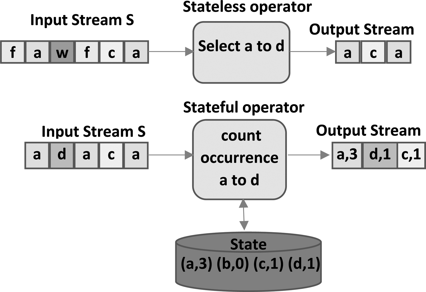end{document} will be null. Figure 3 illustrates our model for both stateless and stateful operators.

OPEN IN VIEWER

OPEN IN VIEWER

FIG. 3.

Operator model.

State model

Stateful operators are normally aggregation operators or join operators and in both of these operators, operations are performed based on some keys, and values of these keys manipulated accordingly. So, we can assume that these keys can be unique for these types of operators. This concept will help us to maintain state of the operator during processing and migration. We define state \documentclass{aastex}\usepackage{amsbsy}\usepackage{amsfonts}\usepackage{amssymb}\usepackage{bm}\usepackage{mathrsfs}\usepackage{pifont}\usepackage{stmaryrd}\usepackage{textcomp}\usepackage{portland, xspace}\usepackage{amsmath, amsxtra}\usepackage{upgreek}\pagestyle{empty}\DeclareMathSizes{10}{9}{7}{6}\begin{document} $${ \theta _o}$$ \end{document} of an operator as a set of key/value pairs, that is, \documentclass{aastex}\usepackage{amsbsy}\usepackage{amsfonts}\usepackage{amssymb}\usepackage{bm}\usepackage{mathrsfs}\usepackage{pifont}\usepackage{stmaryrd}\usepackage{textcomp}\usepackage{portland, xspace}\usepackage{amsmath, amsxtra}\usepackage{upgreek}\pagestyle{empty}\DeclareMathSizes{10}{9}{7}{6}\begin{document} $${ \theta _o}$$ \end{document}  = {(k₁,v₁), …}. Figure 4 illustrates concept of key/value state of an operator.

OPEN IN VIEWER

FIG. 4.

State model.

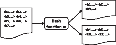
Each key is unique as well as independent of other keys and refers to a corresponding tuple key from the input streams; this will also lead to the independent state of each operator. Its associated value v stores the portion of processing state for that operator. While partitioning an operator to \documentclass{aastex}\usepackage{amsbsy}\usepackage{amsfonts}\usepackage{amssymb}\usepackage{bm}\usepackage{mathrsfs}\usepackage{pifont}\usepackage{stmaryrd}\usepackage{textcomp}\usepackage{portland, xspace}\usepackage{amsmath, amsxtra}\usepackage{upgreek}\pagestyle{empty}\DeclareMathSizes{10}{9}{7}{6}\begin{document} $$\eta$$ \end{document} new nodes, we also have to partition the key space to these new nodes so that each partitioned operator will be working independently from others. We can partition this key space using hash function \documentclass{aastex}\usepackage{amsbsy}\usepackage{amsfonts}\usepackage{amssymb}\usepackage{bm}\usepackage{mathrsfs}\usepackage{pifont}\usepackage{stmaryrd}\usepackage{textcomp}\usepackage{portland, xspace}\usepackage{amsmath, amsxtra}\usepackage{upgreek}\pagestyle{empty}\DeclareMathSizes{10}{9}{7}{6}\begin{document} $$m:k \to [ 1 , \eta ]$$ \end{document} . Figure 5 shows partitioned states.

OPEN IN VIEWER

FIG. 5.

State partition model.

During execution at time t, the stateful operator OP has some memory M = ( \documentclass{aastex}\usepackage{amsbsy}\usepackage{amsfonts}\usepackage{amssymb}\usepackage{bm}\usepackage{mathrsfs}\usepackage{pifont}\usepackage{stmaryrd}\usepackage{textcomp}\usepackage{portland, xspace}\usepackage{amsmath, amsxtra}\usepackage{upgreek}\pagestyle{empty}\DeclareMathSizes{10}{9}{7}{6}\begin{document} $$\theta$$ \end{document} , \documentclass{aastex}\usepackage{amsbsy}\usepackage{amsfonts}\usepackage{amssymb}\usepackage{bm}\usepackage{mathrsfs}\usepackage{pifont}\usepackage{stmaryrd}\usepackage{textcomp}\usepackage{portland, xspace}\usepackage{amsmath, amsxtra}\usepackage{upgreek}\pagestyle{empty}\DeclareMathSizes{10}{9}{7}{6}\begin{document} $${ \kappa _{range}}$$ \end{document} , S) where \documentclass{aastex}\usepackage{amsbsy}\usepackage{amsfonts}\usepackage{amssymb}\usepackage{bm}\usepackage{mathrsfs}\usepackage{pifont}\usepackage{stmaryrd}\usepackage{textcomp}\usepackage{portland, xspace}\usepackage{amsmath, amsxtra}\usepackage{upgreek}\pagestyle{empty}\DeclareMathSizes{10}{9}{7}{6}\begin{document} $${ \kappa _{range}}$$ \end{document} is key range of OP and S is size of memory. During scale out, we have to decompose M = ( \documentclass{aastex}\usepackage{amsbsy}\usepackage{amsfonts}\usepackage{amssymb}\usepackage{bm}\usepackage{mathrsfs}\usepackage{pifont}\usepackage{stmaryrd}\usepackage{textcomp}\usepackage{portland, xspace}\usepackage{amsmath, amsxtra}\usepackage{upgreek}\pagestyle{empty}\DeclareMathSizes{10}{9}{7}{6}\begin{document} $$\theta$$ \end{document} , \documentclass{aastex}\usepackage{amsbsy}\usepackage{amsfonts}\usepackage{amssymb}\usepackage{bm}\usepackage{mathrsfs}\usepackage{pifont}\usepackage{stmaryrd}\usepackage{textcomp}\usepackage{portland, xspace}\usepackage{amsmath, amsxtra}\usepackage{upgreek}\pagestyle{empty}\DeclareMathSizes{10}{9}{7}{6}\begin{document} $${ \kappa _{range}}$$ \end{document} , S) to p partitions where \documentclass{aastex}\usepackage{amsbsy}\usepackage{amsfonts}\usepackage{amssymb}\usepackage{bm}\usepackage{mathrsfs}\usepackage{pifont}\usepackage{stmaryrd}\usepackage{textcomp}\usepackage{portland, xspace}\usepackage{amsmath, amsxtra}\usepackage{upgreek}\pagestyle{empty}\DeclareMathSizes{10}{9}{7}{6}\begin{document} $$p \in \mathbb{Z}$$ \end{document} . When M is decomposed, the resulting new partitions will also become state for newly partitioned operators. Furthermore, the composition of these partitions yields state of OP that is semantically equivalent to original. For two partitions, decomposition is shown in Equation (1). \documentclass{aastex}\usepackage{amsbsy}\usepackage{amsfonts}\usepackage{amssymb}\usepackage{bm}\usepackage{mathrsfs}\usepackage{pifont}\usepackage{stmaryrd}\usepackage{textcomp}\usepackage{portland, xspace}\usepackage{amsmath, amsxtra}\usepackage{upgreek}\pagestyle{empty}\DeclareMathSizes{10}{9}{7}{6}\begin{document} \begin{align*} compose ( {M ^{\displaystyle \prime}_0} , {M ^{\displaystyle \prime}_1} ) = M \leftrightarrow Decompose ( M , p ) = ( {M ^{\displaystyle \prime}_0} , {M ^{\displaystyle \prime}_1} ) \tag{1} \end{align*} \end{document}

We say partitions are semantically correct if read operation for some key \documentclass{aastex}\usepackage{amsbsy}\usepackage{amsfonts}\usepackage{amssymb}\usepackage{bm}\usepackage{mathrsfs}\usepackage{pifont}\usepackage{stmaryrd}\usepackage{textcomp}\usepackage{portland, xspace}\usepackage{amsmath, amsxtra}\usepackage{upgreek}\pagestyle{empty}\DeclareMathSizes{10}{9}{7}{6}\begin{document} $$\kappa$$ \end{document} is performed on partitioned state, the resulting output should be same if read operations are performed on original state. \documentclass{aastex}\usepackage{amsbsy}\usepackage{amsfonts}\usepackage{amssymb}\usepackage{bm}\usepackage{mathrsfs}\usepackage{pifont}\usepackage{stmaryrd}\usepackage{textcomp}\usepackage{portland, xspace}\usepackage{amsmath, amsxtra}\usepackage{upgreek}\pagestyle{empty}\DeclareMathSizes{10}{9}{7}{6}\begin{document} \begin{align*} Let \,M \prime = Decompose ( M , p ) \end{align*} \end{document}

Scale out model

To scale out a bottleneck operator \documentclass{aastex}\usepackage{amsbsy}\usepackage{amsfonts}\usepackage{amssymb}\usepackage{bm}\usepackage{mathrsfs}\usepackage{pifont}\usepackage{stmaryrd}\usepackage{textcomp}\usepackage{portland, xspace}\usepackage{amsmath, amsxtra}\usepackage{upgreek}\pagestyle{empty}\DeclareMathSizes{10}{9}{7}{6}\begin{document} $$O{P_{_i}}$$ \end{document} , we will split it into \documentclass{aastex}\usepackage{amsbsy}\usepackage{amsfonts}\usepackage{amssymb}\usepackage{bm}\usepackage{mathrsfs}\usepackage{pifont}\usepackage{stmaryrd}\usepackage{textcomp}\usepackage{portland, xspace}\usepackage{amsmath, amsxtra}\usepackage{upgreek}\pagestyle{empty}\DeclareMathSizes{10}{9}{7}{6}\begin{document} $$\eta$$ \end{document} new nodes based on the required degree of parallelism to resolve bottleneck. It is given by the following: \documentclass{aastex}\usepackage{amsbsy}\usepackage{amsfonts}\usepackage{amssymb}\usepackage{bm}\usepackage{mathrsfs}\usepackage{pifont}\usepackage{stmaryrd}\usepackage{textcomp}\usepackage{portland, xspace}\usepackage{amsmath, amsxtra}\usepackage{upgreek}\pagestyle{empty}\DeclareMathSizes{10}{9}{7}{6}\begin{document} \begin{align*} O{P_i} = O{P_{i1}} , O{P_{i2}} , ..O{P_{i \eta }} \tag{2} \end{align*} \end{document}

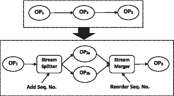
We will also partition state of the operator and its input streams. While partitioning input streams, we will add sequence number so that we can reorder these streams before forwarding these streams to the next operator, as depicted in Figure 6.

OPEN IN VIEWER

FIG. 6.

Operator scale out model.

To handle scale out for any operator OP_i, a fair scale out means that resource allocation should be done well in time to solve the bottleneck.

For OP_i at time t, currently assigned resources \documentclass{aastex}\usepackage{amsbsy}\usepackage{amsfonts}\usepackage{amssymb}\usepackage{bm}\usepackage{mathrsfs}\usepackage{pifont}\usepackage{stmaryrd}\usepackage{textcomp}\usepackage{portland, xspace}\usepackage{amsmath, amsxtra}\usepackage{upgreek}\pagestyle{empty}\DeclareMathSizes{10}{9}{7}{6}\begin{document} $$\Re$$ \end{document} \documentclass{aastex}\usepackage{amsbsy}\usepackage{amsfonts}\usepackage{amssymb}\usepackage{bm}\usepackage{mathrsfs}\usepackage{pifont}\usepackage{stmaryrd}\usepackage{textcomp}\usepackage{portland, xspace}\usepackage{amsmath, amsxtra}\usepackage{upgreek}\pagestyle{empty}\DeclareMathSizes{10}{9}{7}{6}\begin{document} $$cu{r_{op}}$$ \end{document} (t_k) \documentclass{aastex}\usepackage{amsbsy}\usepackage{amsfonts}\usepackage{amssymb}\usepackage{bm}\usepackage{mathrsfs}\usepackage{pifont}\usepackage{stmaryrd}\usepackage{textcomp}\usepackage{portland, xspace}\usepackage{amsmath, amsxtra}\usepackage{upgreek}\pagestyle{empty}\DeclareMathSizes{10}{9}{7}{6}\begin{document} $$\in$$ \end{document} [0, t_k] are consumed, which can be cumulatively shown in Equation (3). \documentclass{aastex}\usepackage{amsbsy}\usepackage{amsfonts}\usepackage{amssymb}\usepackage{bm}\usepackage{mathrsfs}\usepackage{pifont}\usepackage{stmaryrd}\usepackage{textcomp}\usepackage{portland, xspace}\usepackage{amsmath, amsxtra}\usepackage{upgreek}\pagestyle{empty}\DeclareMathSizes{10}{9}{7}{6}\begin{document} \begin{align*} \Re cu{r_{op}} ( {t_k} ) = \int_0^{{t_k}} cu{r_{op}} ( t ) dt \tag{3} \end{align*} \end{document}

where cur_op(t) are the resources currently consumed by OP_i at time t. To resolve the bottleneck, the total number of needed resources \documentclass{aastex}\usepackage{amsbsy}\usepackage{amsfonts}\usepackage{amssymb}\usepackage{bm}\usepackage{mathrsfs}\usepackage{pifont}\usepackage{stmaryrd}\usepackage{textcomp}\usepackage{portland, xspace}\usepackage{amsmath, amsxtra}\usepackage{upgreek}\pagestyle{empty}\DeclareMathSizes{10}{9}{7}{6}\begin{document} $$\Re nee{d_{op}}$$ \end{document} (t_k) \documentclass{aastex}\usepackage{amsbsy}\usepackage{amsfonts}\usepackage{amssymb}\usepackage{bm}\usepackage{mathrsfs}\usepackage{pifont}\usepackage{stmaryrd}\usepackage{textcomp}\usepackage{portland, xspace}\usepackage{amsmath, amsxtra}\usepackage{upgreek}\pagestyle{empty}\DeclareMathSizes{10}{9}{7}{6}\begin{document} $$\in$$ \end{document} [0, t_k] can be cumulatively defined as Equation (4). \documentclass{aastex}\usepackage{amsbsy}\usepackage{amsfonts}\usepackage{amssymb}\usepackage{bm}\usepackage{mathrsfs}\usepackage{pifont}\usepackage{stmaryrd}\usepackage{textcomp}\usepackage{portland, xspace}\usepackage{amsmath, amsxtra}\usepackage{upgreek}\pagestyle{empty}\DeclareMathSizes{10}{9}{7}{6}\begin{document} \begin{align*} \Re nee{d_{op}} ( {t_k} ) = \int_0^{{t_k}} nee{d_{op}} ( t ) dt \tag{4} \end{align*} \end{document}

where need_op(t) is total required resources by OP_i at time t. The fairness degree \documentclass{aastex}\usepackage{amsbsy}\usepackage{amsfonts}\usepackage{amssymb}\usepackage{bm}\usepackage{mathrsfs}\usepackage{pifont}\usepackage{stmaryrd}\usepackage{textcomp}\usepackage{portland, xspace}\usepackage{amsmath, amsxtra}\usepackage{upgreek}\pagestyle{empty}\DeclareMathSizes{10}{9}{7}{6}\begin{document} $$f{d_{op}}$$ \end{document} for operator OP_i at time t_k is given by Equation (5). \documentclass{aastex}\usepackage{amsbsy}\usepackage{amsfonts}\usepackage{amssymb}\usepackage{bm}\usepackage{mathrsfs}\usepackage{pifont}\usepackage{stmaryrd}\usepackage{textcomp}\usepackage{portland, xspace}\usepackage{amsmath, amsxtra}\usepackage{upgreek}\pagestyle{empty}\DeclareMathSizes{10}{9}{7}{6}\begin{document} \begin{align*} f { d_ { op } } ( { t_k } ) = { \frac { \Re cu { r_ { op } } ( { t_k } ) } { \Re nee { d_ { op } } ( { t_k } ) } } = { \frac { \int_0^ { { t_k } } cu { r_ { op } } ( t ) dt } { \int_0^ { { t_k } } nee { d_ { op } } ( t ) dt } } \tag { 5 } \end{align*} \end{document}

To resolve a bottleneck, total needed resources \documentclass{aastex}\usepackage{amsbsy}\usepackage{amsfonts}\usepackage{amssymb}\usepackage{bm}\usepackage{mathrsfs}\usepackage{pifont}\usepackage{stmaryrd}\usepackage{textcomp}\usepackage{portland, xspace}\usepackage{amsmath, amsxtra}\usepackage{upgreek}\pagestyle{empty}\DeclareMathSizes{10}{9}{7}{6}\begin{document} $$\Re nee{d_{op}}$$ \end{document} (t_k) are always greater than currently assigned resources \documentclass{aastex}\usepackage{amsbsy}\usepackage{amsfonts}\usepackage{amssymb}\usepackage{bm}\usepackage{mathrsfs}\usepackage{pifont}\usepackage{stmaryrd}\usepackage{textcomp}\usepackage{portland, xspace}\usepackage{amsmath, amsxtra}\usepackage{upgreek}\pagestyle{empty}\DeclareMathSizes{10}{9}{7}{6}\begin{document} $$\Re cu{r_{op}}$$ \end{document} (t_k), and hence, the fairness degree \documentclass{aastex}\usepackage{amsbsy}\usepackage{amsfonts}\usepackage{amssymb}\usepackage{bm}\usepackage{mathrsfs}\usepackage{pifont}\usepackage{stmaryrd}\usepackage{textcomp}\usepackage{portland, xspace}\usepackage{amsmath, amsxtra}\usepackage{upgreek}\pagestyle{empty}\DeclareMathSizes{10}{9}{7}{6}\begin{document} $$f{d_{op}}$$ \end{document} (t_k) \documentclass{aastex}\usepackage{amsbsy}\usepackage{amsfonts}\usepackage{amssymb}\usepackage{bm}\usepackage{mathrsfs}\usepackage{pifont}\usepackage{stmaryrd}\usepackage{textcomp}\usepackage{portland, xspace}\usepackage{amsmath, amsxtra}\usepackage{upgreek}\pagestyle{empty}\DeclareMathSizes{10}{9}{7}{6}\begin{document} $$\in$$ \end{document} [0, 1] holds. It shows that if \documentclass{aastex}\usepackage{amsbsy}\usepackage{amsfonts}\usepackage{amssymb}\usepackage{bm}\usepackage{mathrsfs}\usepackage{pifont}\usepackage{stmaryrd}\usepackage{textcomp}\usepackage{portland, xspace}\usepackage{amsmath, amsxtra}\usepackage{upgreek}\pagestyle{empty}\DeclareMathSizes{10}{9}{7}{6}\begin{document} $$f{d_{op}}$$ \end{document} (t_k) = 1, then at time t_k, all needed resources are provided, while a 0 value shows that the operator is still bottleneck because needed resources are not provided yet.

To obtain average fairness degree for an application [i.e., \documentclass{aastex}\usepackage{amsbsy}\usepackage{amsfonts}\usepackage{amssymb}\usepackage{bm}\usepackage{mathrsfs}\usepackage{pifont}\usepackage{stmaryrd}\usepackage{textcomp}\usepackage{portland, xspace}\usepackage{amsmath, amsxtra}\usepackage{upgreek}\pagestyle{empty}\DeclareMathSizes{10}{9}{7}{6}\begin{document} $$F{d_{app}}$$ \end{document} (t_k)] in which n operators are bottleneck at time t_k, as given by Equation (6). \documentclass{aastex}\usepackage{amsbsy}\usepackage{amsfonts}\usepackage{amssymb}\usepackage{bm}\usepackage{mathrsfs}\usepackage{pifont}\usepackage{stmaryrd}\usepackage{textcomp}\usepackage{portland, xspace}\usepackage{amsmath, amsxtra}\usepackage{upgreek}\pagestyle{empty}\DeclareMathSizes{10}{9}{7}{6}\begin{document} \begin{align*} F { d_ { app } } { ( _k } ) = \frac { 1 } { n } \sum \limits_ { n = 1 } ^n f { d_ { opi } } ( { t_k } ) \quad \quad where \quad \quad f { d_ { op } } ( { t_k } ) \in [ 0 , 1 ] \tag { 6 } \end{align*} \end{document}

Active backup

Our active backup server technique is not as costly as that of a backup server for each primary server; rather, we are using this technique with slight changes. During bottleneck detection, when an operator approaches at alarming_threshold ( \documentclass{aastex}\usepackage{amsbsy}\usepackage{amsfonts}\usepackage{amssymb}\usepackage{bm}\usepackage{mathrsfs}\usepackage{pifont}\usepackage{stmaryrd}\usepackage{textcomp}\usepackage{portland, xspace}\usepackage{amsmath, amsxtra}\usepackage{upgreek}\pagestyle{empty}\DeclareMathSizes{10}{9}{7}{6}\begin{document} $${ \delta \prime _2}$$ \end{document} ), scale out is performed by starting secondary servers using SE module. This module will be responsible for partitioning state and input streams of primary server to new nodes. The benefit of active backup technique is that there is no need to store backup on upstream servers in the form of checkpoints, which may result in overloading the upstream server also. The other benefit is that there is no need to replay some tuples to achieve state similar to one running on primary server, which will result in time saving as well as delay avoidance. One problem of active backup technique is that it doubles the cost, but in our implementation the SE will not start any new nodes until we detect some operator approaching near to the bottleneck. So this means that we are not always running an extra server as backup of some primary server, rather we start an extra server only when it is required.

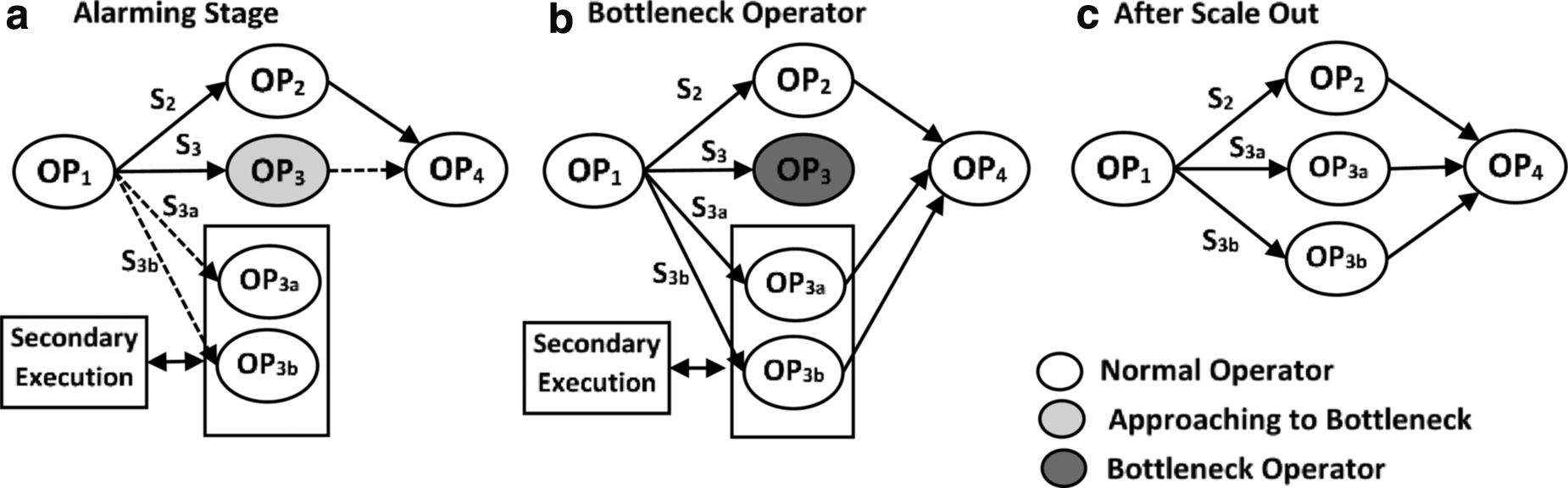
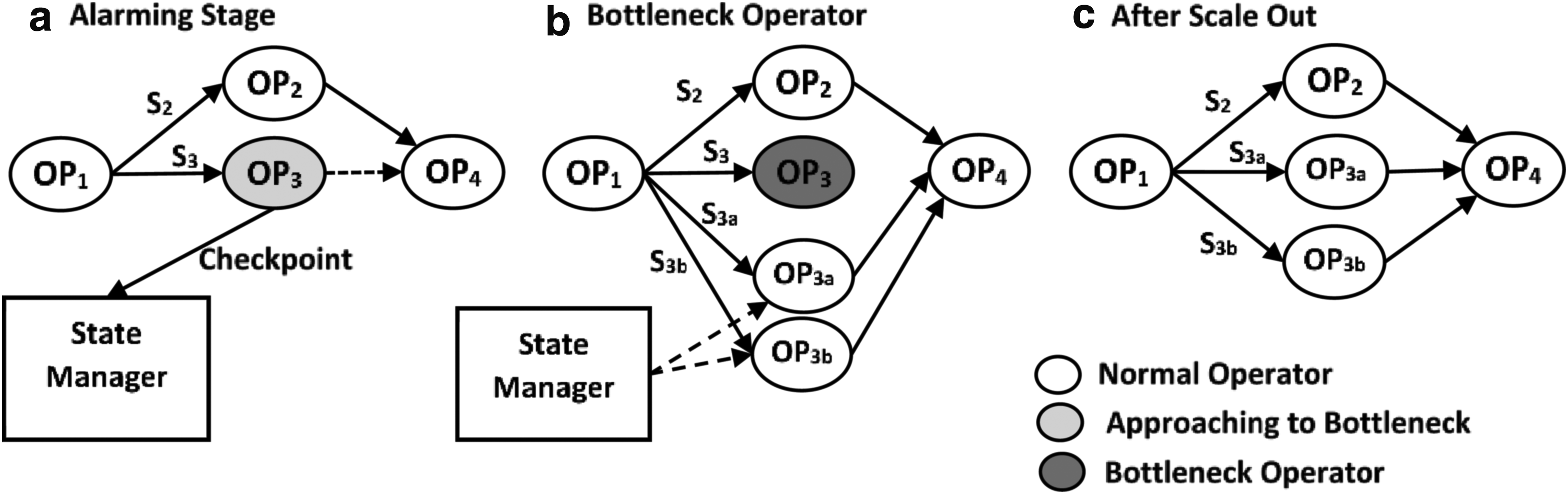
In Figure 7, the execution plan is shown with addition of SE module. As we are continuously tracking load of the node, suppose workload of \documentclass{aastex}\usepackage{amsbsy}\usepackage{amsfonts}\usepackage{amssymb}\usepackage{bm}\usepackage{mathrsfs}\usepackage{pifont}\usepackage{stmaryrd}\usepackage{textcomp}\usepackage{portland, xspace}\usepackage{amsmath, amsxtra}\usepackage{upgreek}\pagestyle{empty}\DeclareMathSizes{10}{9}{7}{6}\begin{document} $$O{P_3}$$ \end{document} is started to increase and at time t this operator approaches alarming_threshold ( \documentclass{aastex}\usepackage{amsbsy}\usepackage{amsfonts}\usepackage{amssymb}\usepackage{bm}\usepackage{mathrsfs}\usepackage{pifont}\usepackage{stmaryrd}\usepackage{textcomp}\usepackage{portland, xspace}\usepackage{amsmath, amsxtra}\usepackage{upgreek}\pagestyle{empty}\DeclareMathSizes{10}{9}{7}{6}\begin{document} $${ \delta \prime _2}$$ \end{document} ), now SE will start scale out by adding two new nodes OP_3a and OP_3b and when OP₃ reaches scale_out_threshold, SE will replace primary server with new nodes. This active backup is not working all the time (i.e., from start of \documentclass{aastex}\usepackage{amsbsy}\usepackage{amsfonts}\usepackage{amssymb}\usepackage{bm}\usepackage{mathrsfs}\usepackage{pifont}\usepackage{stmaryrd}\usepackage{textcomp}\usepackage{portland, xspace}\usepackage{amsmath, amsxtra}\usepackage{upgreek}\pagestyle{empty}\DeclareMathSizes{10}{9}{7}{6}\begin{document} $$O{P_3}$$ \end{document} ) and we are starting this active backup when OP₃ will reach ( \documentclass{aastex}\usepackage{amsbsy}\usepackage{amsfonts}\usepackage{amssymb}\usepackage{bm}\usepackage{mathrsfs}\usepackage{pifont}\usepackage{stmaryrd}\usepackage{textcomp}\usepackage{portland, xspace}\usepackage{amsmath, amsxtra}\usepackage{upgreek}\pagestyle{empty}\DeclareMathSizes{10}{9}{7}{6}\begin{document} $${ \delta \prime _2}$$ \end{document} ); this will help us to reduce infrastructure cost and at the same time by using SE we are aiming to achieve zero latency in case of operator bottleneck.

OPEN IN VIEWER

FIG. 7.

(a–c) Active backup and secondary execution.

Regarding working of SE, first, we will copy state from primary node running OP₃ and partition it further on two new nodes as OP_3a and OP_3b so that we can divide load and process OP₃ with more speed (the number of new nodes can be increased or decreased as per requirement). We also have to partition data stream S₃ into S_3a and S_3b accordingly so that both new operators should get their respective data streams for processing tuples. We should take care of splitting stream from tuple t_i with time \documentclass{aastex}\usepackage{amsbsy}\usepackage{amsfonts}\usepackage{amssymb}\usepackage{bm}\usepackage{mathrsfs}\usepackage{pifont}\usepackage{stmaryrd}\usepackage{textcomp}\usepackage{portland, xspace}\usepackage{amsmath, amsxtra}\usepackage{upgreek}\pagestyle{empty}\DeclareMathSizes{10}{9}{7}{6}\begin{document} $${ \tau _i}$$ \end{document} , which is the time when the state \documentclass{aastex}\usepackage{amsbsy}\usepackage{amsfonts}\usepackage{amssymb}\usepackage{bm}\usepackage{mathrsfs}\usepackage{pifont}\usepackage{stmaryrd}\usepackage{textcomp}\usepackage{portland, xspace}\usepackage{amsmath, amsxtra}\usepackage{upgreek}\pagestyle{empty}\DeclareMathSizes{10}{9}{7}{6}\begin{document} $${ \theta _o}$$ \end{document} is copied to SE from OP₃.

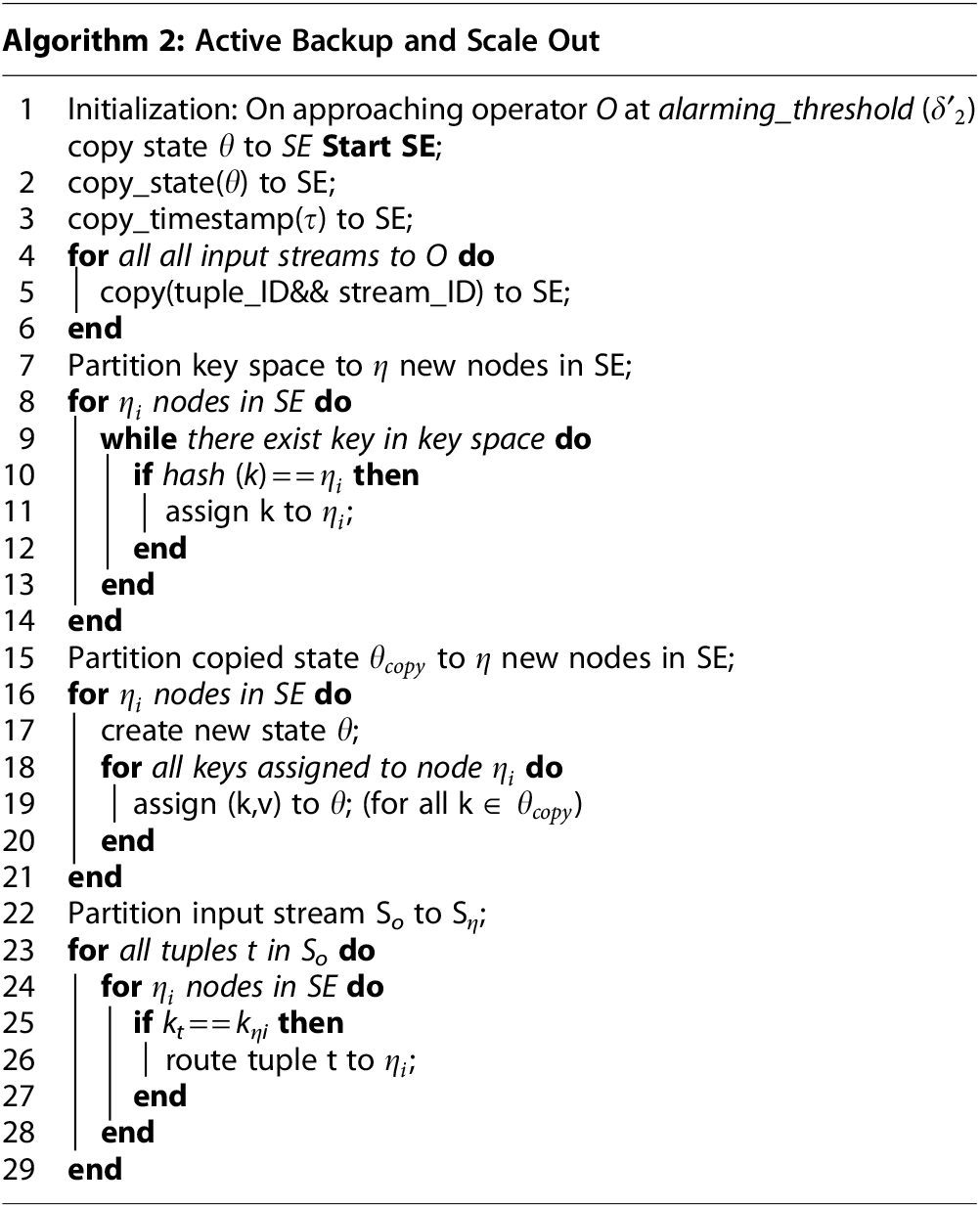
Algorithm 2 describes how state management is performed by first copying state and then by partitioning key space, the state itself, and incoming streams to new nodes in SE. During initialization when an operator reaches alarming_threshold, SE is started and copies state and time stamp \documentclass{aastex}\usepackage{amsbsy}\usepackage{amsfonts}\usepackage{amssymb}\usepackage{bm}\usepackage{mathrsfs}\usepackage{pifont}\usepackage{stmaryrd}\usepackage{textcomp}\usepackage{portland, xspace}\usepackage{amsmath, amsxtra}\usepackage{upgreek}\pagestyle{empty}\DeclareMathSizes{10}{9}{7}{6}\begin{document} $$\tau$$ \end{document} to SE (lines 1–3). As a single operator can process multiple input streams, there is a need to copy stream_ID and tuple_ID of respective streams to SE; this is performed using a loop in lines 4–6. After copying now, we have to divide key space from lines 7 to 14 and this is done by using a hash function to partition key space to \documentclass{aastex}\usepackage{amsbsy}\usepackage{amsfonts}\usepackage{amssymb}\usepackage{bm}\usepackage{mathrsfs}\usepackage{pifont}\usepackage{stmaryrd}\usepackage{textcomp}\usepackage{portland, xspace}\usepackage{amsmath, amsxtra}\usepackage{upgreek}\pagestyle{empty}\DeclareMathSizes{10}{9}{7}{6}\begin{document} $$\eta$$ \end{document} new nodes, all keys are partitioned evenly to new nodes in SE setup so that workload is divided evenly among all new nodes. In line 17, a new state \documentclass{aastex}\usepackage{amsbsy}\usepackage{amsfonts}\usepackage{amssymb}\usepackage{bm}\usepackage{mathrsfs}\usepackage{pifont}\usepackage{stmaryrd}\usepackage{textcomp}\usepackage{portland, xspace}\usepackage{amsmath, amsxtra}\usepackage{upgreek}\pagestyle{empty}\DeclareMathSizes{10}{9}{7}{6}\begin{document} $$\theta$$ \end{document} is created on each new node and we partitioned copied state \documentclass{aastex}\usepackage{amsbsy}\usepackage{amsfonts}\usepackage{amssymb}\usepackage{bm}\usepackage{mathrsfs}\usepackage{pifont}\usepackage{stmaryrd}\usepackage{textcomp}\usepackage{portland, xspace}\usepackage{amsmath, amsxtra}\usepackage{upgreek}\pagestyle{empty}\DeclareMathSizes{10}{9}{7}{6}\begin{document} $${ \theta _{copy}}$$ \end{document} to \documentclass{aastex}\usepackage{amsbsy}\usepackage{amsfonts}\usepackage{amssymb}\usepackage{bm}\usepackage{mathrsfs}\usepackage{pifont}\usepackage{stmaryrd}\usepackage{textcomp}\usepackage{portland, xspace}\usepackage{amsmath, amsxtra}\usepackage{upgreek}\pagestyle{empty}\DeclareMathSizes{10}{9}{7}{6}\begin{document} $$\eta$$ \end{document} new nodes and assigned respective key value pairs (k,v) to the newly created state \documentclass{aastex}\usepackage{amsbsy}\usepackage{amsfonts}\usepackage{amssymb}\usepackage{bm}\usepackage{mathrsfs}\usepackage{pifont}\usepackage{stmaryrd}\usepackage{textcomp}\usepackage{portland, xspace}\usepackage{amsmath, amsxtra}\usepackage{upgreek}\pagestyle{empty}\DeclareMathSizes{10}{9}{7}{6}\begin{document} $$\theta$$ \end{document} (this is performed in lines 18 and 19). Finally, we have partitioned input streams of operator to available nodes in SE from lines 22 to 29; we have to be careful here that from incoming streams all tuples t should be routed to that \documentclass{aastex}\usepackage{amsbsy}\usepackage{amsfonts}\usepackage{amssymb}\usepackage{bm}\usepackage{mathrsfs}\usepackage{pifont}\usepackage{stmaryrd}\usepackage{textcomp}\usepackage{portland, xspace}\usepackage{amsmath, amsxtra}\usepackage{upgreek}\pagestyle{empty}\DeclareMathSizes{10}{9}{7}{6}\begin{document} $${ \eta _i}$$ \end{document} node, having relevant partition of key space.

OPEN IN VIEWER

Checkpointing and scale out

Checkpointing saves state of operator to some storage, which allows it to be further processed in the form of scaling out an operator or restarting some failed operator from that stored state; this process is known as checkpointing. Castro Fernandez et al. ⁶ performed scale out and fault tolerance in stream processing using operator state management, saying that operator state can be checkpointed periodically by the SPS and backed up to upstream servers. After bottleneck of some operators, this backup can be used to scale out, or in case of failure, recovery can be performed. The problem with this approach is that system is performing continuous checkpointing for every operator, which introduces an extra overhead on each operator. Also, the backup is stored on some upstream operator, which puts extra load on upstream operators. To handle this problem we are proposing a solution where continuous checkpointing is not allowed for every operator; rather, we are checkpointing only those operators that are approaching the alarming_threshold ( \documentclass{aastex}\usepackage{amsbsy}\usepackage{amsfonts}\usepackage{amssymb}\usepackage{bm}\usepackage{mathrsfs}\usepackage{pifont}\usepackage{stmaryrd}\usepackage{textcomp}\usepackage{portland, xspace}\usepackage{amsmath, amsxtra}\usepackage{upgreek}\pagestyle{empty}\DeclareMathSizes{10}{9}{7}{6}\begin{document} $${ \delta \prime _2}$$ \end{document} ) stage, and also not storing backup on upstream server.

We have introduced an SM module for the checkpointing and scale out technique to scale out the bottleneck operator. SM will handle the state first by storing its backup, which will be obtained by checkpointing the state and afterward partitioning this state to new nodes. The checkpointed state will contain ( \documentclass{aastex}\usepackage{amsbsy}\usepackage{amsfonts}\usepackage{amssymb}\usepackage{bm}\usepackage{mathrsfs}\usepackage{pifont}\usepackage{stmaryrd}\usepackage{textcomp}\usepackage{portland, xspace}\usepackage{amsmath, amsxtra}\usepackage{upgreek}\pagestyle{empty}\DeclareMathSizes{10}{9}{7}{6}\begin{document} $${ \theta _o}$$ \end{document} , \documentclass{aastex}\usepackage{amsbsy}\usepackage{amsfonts}\usepackage{amssymb}\usepackage{bm}\usepackage{mathrsfs}\usepackage{pifont}\usepackage{stmaryrd}\usepackage{textcomp}\usepackage{portland, xspace}\usepackage{amsmath, amsxtra}\usepackage{upgreek}\pagestyle{empty}\DeclareMathSizes{10}{9}{7}{6}\begin{document} $${ \tau _o}$$ \end{document} , \documentclass{aastex}\usepackage{amsbsy}\usepackage{amsfonts}\usepackage{amssymb}\usepackage{bm}\usepackage{mathrsfs}\usepackage{pifont}\usepackage{stmaryrd}\usepackage{textcomp}\usepackage{portland, xspace}\usepackage{amsmath, amsxtra}\usepackage{upgreek}\pagestyle{empty}\DeclareMathSizes{10}{9}{7}{6}\begin{document} $${ \beta _{_o}}$$ \end{document} ), where \documentclass{aastex}\usepackage{amsbsy}\usepackage{amsfonts}\usepackage{amssymb}\usepackage{bm}\usepackage{mathrsfs}\usepackage{pifont}\usepackage{stmaryrd}\usepackage{textcomp}\usepackage{portland, xspace}\usepackage{amsmath, amsxtra}\usepackage{upgreek}\pagestyle{empty}\DeclareMathSizes{10}{9}{7}{6}\begin{document} $${ \theta _o}$$ \end{document} is state of operator, \documentclass{aastex}\usepackage{amsbsy}\usepackage{amsfonts}\usepackage{amssymb}\usepackage{bm}\usepackage{mathrsfs}\usepackage{pifont}\usepackage{stmaryrd}\usepackage{textcomp}\usepackage{portland, xspace}\usepackage{amsmath, amsxtra}\usepackage{upgreek}\pagestyle{empty}\DeclareMathSizes{10}{9}{7}{6}\begin{document} $${ \tau _o}$$ \end{document} is time stamp of most recent tuple, which is processed and reflected in state, and \documentclass{aastex}\usepackage{amsbsy}\usepackage{amsfonts}\usepackage{amssymb}\usepackage{bm}\usepackage{mathrsfs}\usepackage{pifont}\usepackage{stmaryrd}\usepackage{textcomp}\usepackage{portland, xspace}\usepackage{amsmath, amsxtra}\usepackage{upgreek}\pagestyle{empty}\DeclareMathSizes{10}{9}{7}{6}\begin{document} $${ \beta _o}$$ \end{document} is buffer attached to the operator to temporarily hold tuples flowing from upstream operator to downstream operator. Remember the system will not always be doing checkpointing. The process of checkpointing will start when the operator approaches alarming_threshold ( \documentclass{aastex}\usepackage{amsbsy}\usepackage{amsfonts}\usepackage{amssymb}\usepackage{bm}\usepackage{mathrsfs}\usepackage{pifont}\usepackage{stmaryrd}\usepackage{textcomp}\usepackage{portland, xspace}\usepackage{amsmath, amsxtra}\usepackage{upgreek}\pagestyle{empty}\DeclareMathSizes{10}{9}{7}{6}\begin{document} $${ \delta \prime _2}$$ \end{document} ). The checkpoint state is executed now onward asynchronously and triggered at every checkpointing interval c, or after a user-defined event, for example, when the state has changed significantly. After the operator state was backed up, the processed tuples from output buffers in upstream operators can be discarded because they are no longer required to process.

Suppose, as shown in Figure 8, OP₃ is near bottleneck, which means it is at alarming_threshold ( \documentclass{aastex}\usepackage{amsbsy}\usepackage{amsfonts}\usepackage{amssymb}\usepackage{bm}\usepackage{mathrsfs}\usepackage{pifont}\usepackage{stmaryrd}\usepackage{textcomp}\usepackage{portland, xspace}\usepackage{amsmath, amsxtra}\usepackage{upgreek}\pagestyle{empty}\DeclareMathSizes{10}{9}{7}{6}\begin{document} $${ \delta \prime _2}$$ \end{document} ), we have to start checkpointing for this operator to SM, and when this operator reaches at scale_out_threshold ( \documentclass{aastex}\usepackage{amsbsy}\usepackage{amsfonts}\usepackage{amssymb}\usepackage{bm}\usepackage{mathrsfs}\usepackage{pifont}\usepackage{stmaryrd}\usepackage{textcomp}\usepackage{portland, xspace}\usepackage{amsmath, amsxtra}\usepackage{upgreek}\pagestyle{empty}\DeclareMathSizes{10}{9}{7}{6}\begin{document} $${ \delta _2}$$ \end{document} ), SM will start new nodes OP_3a and OP_3b and partition the checkpointed state and tuples stored in \documentclass{aastex}\usepackage{amsbsy}\usepackage{amsfonts}\usepackage{amssymb}\usepackage{bm}\usepackage{mathrsfs}\usepackage{pifont}\usepackage{stmaryrd}\usepackage{textcomp}\usepackage{portland, xspace}\usepackage{amsmath, amsxtra}\usepackage{upgreek}\pagestyle{empty}\DeclareMathSizes{10}{9}{7}{6}\begin{document} $${ \beta _o}$$ \end{document} to new nodes and process these tuples. At the same time, also partition input streams and route the partitioned streams to new nodes and start processing new nodes.

OPEN IN VIEWER

FIG. 8.

(a–c) Checkpointing and scale out.

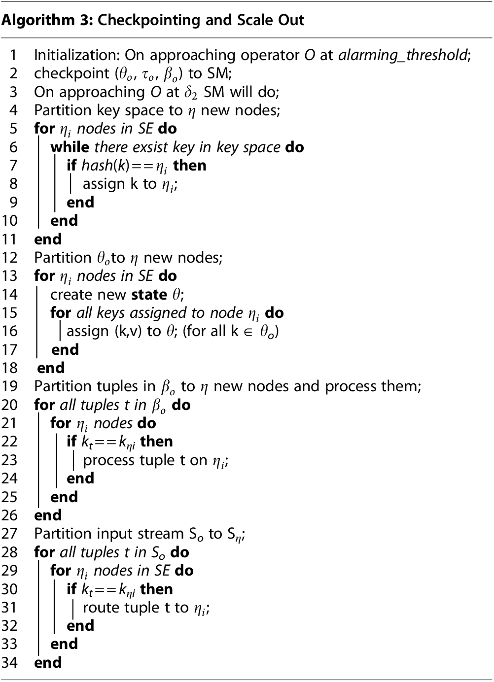
Algorithm 3 describes how the process of checkpointing and scale out works. On approaching some OP at alarming_threshold ( \documentclass{aastex}\usepackage{amsbsy}\usepackage{amsfonts}\usepackage{amssymb}\usepackage{bm}\usepackage{mathrsfs}\usepackage{pifont}\usepackage{stmaryrd}\usepackage{textcomp}\usepackage{portland, xspace}\usepackage{amsmath, amsxtra}\usepackage{upgreek}\pagestyle{empty}\DeclareMathSizes{10}{9}{7}{6}\begin{document} $${ \delta \prime _2}$$ \end{document} ), we start backing up its state using checkpointed state ( \documentclass{aastex}\usepackage{amsbsy}\usepackage{amsfonts}\usepackage{amssymb}\usepackage{bm}\usepackage{mathrsfs}\usepackage{pifont}\usepackage{stmaryrd}\usepackage{textcomp}\usepackage{portland, xspace}\usepackage{amsmath, amsxtra}\usepackage{upgreek}\pagestyle{empty}\DeclareMathSizes{10}{9}{7}{6}\begin{document} $${ \theta _o}$$ \end{document} , \documentclass{aastex}\usepackage{amsbsy}\usepackage{amsfonts}\usepackage{amssymb}\usepackage{bm}\usepackage{mathrsfs}\usepackage{pifont}\usepackage{stmaryrd}\usepackage{textcomp}\usepackage{portland, xspace}\usepackage{amsmath, amsxtra}\usepackage{upgreek}\pagestyle{empty}\DeclareMathSizes{10}{9}{7}{6}\begin{document} $${ \tau _o}$$ \end{document} , \documentclass{aastex}\usepackage{amsbsy}\usepackage{amsfonts}\usepackage{amssymb}\usepackage{bm}\usepackage{mathrsfs}\usepackage{pifont}\usepackage{stmaryrd}\usepackage{textcomp}\usepackage{portland, xspace}\usepackage{amsmath, amsxtra}\usepackage{upgreek}\pagestyle{empty}\DeclareMathSizes{10}{9}{7}{6}\begin{document} $${ \beta _o}$$ \end{document} ) and store it to SM (line 2). When operator O approaches to scale_out_threshold ( \documentclass{aastex}\usepackage{amsbsy}\usepackage{amsfonts}\usepackage{amssymb}\usepackage{bm}\usepackage{mathrsfs}\usepackage{pifont}\usepackage{stmaryrd}\usepackage{textcomp}\usepackage{portland, xspace}\usepackage{amsmath, amsxtra}\usepackage{upgreek}\pagestyle{empty}\DeclareMathSizes{10}{9}{7}{6}\begin{document} $${ \delta _2}$$ \end{document} ), the SM will start partitioning its key space to \documentclass{aastex}\usepackage{amsbsy}\usepackage{amsfonts}\usepackage{amssymb}\usepackage{bm}\usepackage{mathrsfs}\usepackage{pifont}\usepackage{stmaryrd}\usepackage{textcomp}\usepackage{portland, xspace}\usepackage{amsmath, amsxtra}\usepackage{upgreek}\pagestyle{empty}\DeclareMathSizes{10}{9}{7}{6}\begin{document} $$\eta$$ \end{document} new nodes by using a hashing mechanism (lines 4–11). Now SM will partition state of operator by obtaining a copy from the most recent checkpointed state; for this purpose, SM first creates an empty state on each new node (line 14) and then assigns key value pairs from \documentclass{aastex}\usepackage{amsbsy}\usepackage{amsfonts}\usepackage{amssymb}\usepackage{bm}\usepackage{mathrsfs}\usepackage{pifont}\usepackage{stmaryrd}\usepackage{textcomp}\usepackage{portland, xspace}\usepackage{amsmath, amsxtra}\usepackage{upgreek}\pagestyle{empty}\DeclareMathSizes{10}{9}{7}{6}\begin{document} $${ \theta _0}$$ \end{document} to a newly created state (line 16), this will complete state partitioning process. Now we will distribute tuples stored in buffers \documentclass{aastex}\usepackage{amsbsy}\usepackage{amsfonts}\usepackage{amssymb}\usepackage{bm}\usepackage{mathrsfs}\usepackage{pifont}\usepackage{stmaryrd}\usepackage{textcomp}\usepackage{portland, xspace}\usepackage{amsmath, amsxtra}\usepackage{upgreek}\pagestyle{empty}\DeclareMathSizes{10}{9}{7}{6}\begin{document} $${ \beta _o}$$ \end{document} toward the respective node (line 22) and process these tuples on that node (line 23). Now new nodes are ready to process input streams, but we will partition the input stream S_o to \documentclass{aastex}\usepackage{amsbsy}\usepackage{amsfonts}\usepackage{amssymb}\usepackage{bm}\usepackage{mathrsfs}\usepackage{pifont}\usepackage{stmaryrd}\usepackage{textcomp}\usepackage{portland, xspace}\usepackage{amsmath, amsxtra}\usepackage{upgreek}\pagestyle{empty}\DeclareMathSizes{10}{9}{7}{6}\begin{document} $${S_ \eta }$$ \end{document} (lines 27–34). New nodes have started processing input streams for which they will produce some output streams; we have to make sure when output streams of new nodes and output streams of the bottleneck nodes are same, and once this is achieved, we will stop bottleneck node and route output streams of new nodes to downstream operator.

OPEN IN VIEWER

Apache storm

Some key abstractions in Apache Storm include tuple, which is an ordered list of key/value pairs and a stream that is an unbounded sequence of tuples. A streaming application is represented by a topology called DAG that contains operators as nodes and links between operators denote flow of streams. Operators can be spouts or bolts, which contain actual processing logic; spouts represent the source of streams while bolts process input streams to produce results. Bolt can run functions such as filter, aggregate, join, or connectivity to some database.

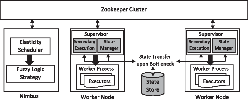
There are two types of nodes in Storm Nimbus and Supervisor. Nimbus is master node and is responsible for scheduling tasks to worker nodes. Once scheduling is done, the plan is communicated to worker nodes using ZooKeeper, ¹⁰ which is a shared memory service for communication among distributed systems. Supervisor is a slave node having one or more worker processes and it assigns tasks to workers, each task may run as single or multiple executors. A topology is submitted to Nimbus, which gathers tasks to be executed and distributes these tasks to available Supervisors. Storm parallelizes operators to increase the throughput.

Bolts are by default stateless and to handle stateful operators it requires maintaining state in the memory as Map or any other data structure, but when worker or node fails this state is lost. Currently, state persistence is only achieved through regular checkpointing to a remote Redis ¹¹ store. This feature was introduced in Storm 1.0.0, which has its own limitations, as described in the Bottleneck Detection section.

Integration with storm

Our proposed dynamic state management framework is a lightweight module integrated with Storm to check for bottleneck operator and then scale it out by handling state using our proposed approaches, that is, active backup and checkpointing and scale out. Currently, Storm has four kinds of built-in schedulers and also allows implementing your own scheduler to assign executors to workers. We run a customized scheduler by configuring the class to use the “storm.scheduler” config in storm.yaml and also implemented IScheduler interface in Storm default scheduler, hence replacing default scheduler of Storm.

We used scheduler and fuzzy logic strategy modules from our previous work by Zhai and Xu. ⁸ The SE module is responsible for scaling operations related to our active backup technique, while SM module will handle scaling operations for checkpointing and scale out technique. We have also added modules for state storage and retrieval where we have used in-memory data store Redis. ¹¹ Figure 9 shows the architecture of system integration with Storm.

OPEN IN VIEWER

FIG. 9.

Integration with Storm, where newly added modules are highlighted in gray.

Experimental setup

We ran the experiments using Storm v1.1.2, using a cluster of three nodes, each configured with three worker nodes, and so, a total of nine workers are running. Among the three nodes, one machine is with 6 GB RAM and the other two having 4 GB RAM with Core i5 CPU at 2.30 GHz processors. We ran additionally Nimbus and Redis services on machine with 6 GB of RAM.

To test the effectiveness of our approach, we tested an application of frequent pattern detection, and for pattern generation, we have used an offline stream data producer, JSON-Data-Generator (JDG). ¹² This is an open-source project, which can generate a real-time stream of JSON data. We have integrated it with our application to generate different patterns, and a detector operator (stateful operator) maintains a counter for the appearances of these patterns.

Results

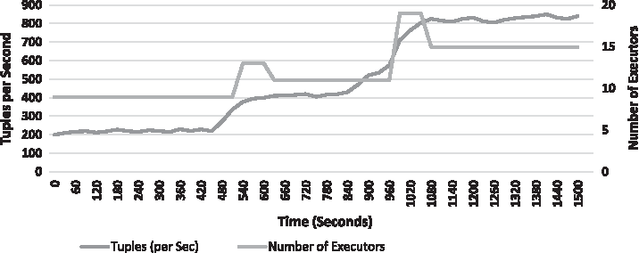
To test for elasticity, we have tested both of our techniques in the same manner described below. To test for elasticity, we configured stateful bolt to increase the number of executors to double in case of bottleneck, starting at two executors for spout and five executors for stateless bolt and two executors for stateful bolt. We started with simple workload 200 tuples per second and increased it continuously by almost doubling the rate after every 500 seconds. Figure 10 shows scale out for our active backup technique. It depicts that each time we increased load, bottleneck was detected and scale out operation is performed. After scaling it out, the number of executors was increased with respect to the scale out ratio set for stateful bolt. During the first scale out operation, the number of executors was raised to 13, but when the SE (in case of active backup) or in case of checkpointing option, our newly added executors taken over the bottlenecked operator number of executors became 11. This is because in our implementation we continue to run bottleneck operator until backup has taken over. Once backup nodes started to work as normal nodes, bottleneck operators were stopped to release the resources.

OPEN IN VIEWER

FIG. 10.

Scale out for active backup.

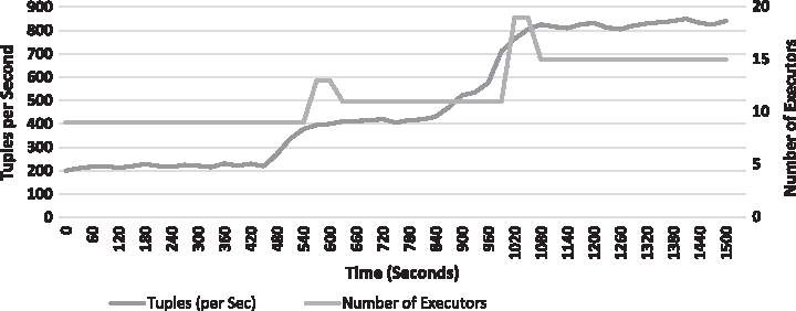
Figure 11 shows scale out for our checkpointing technique. Scale out behavior for both techniques is the same, but there is only difference of resource consumption. Checkpointing techniques use less resources compared with the active backup technique.

OPEN IN VIEWER

FIG. 11.

Scale out for checkpointing.

The fuzzy logic module is working in the system to find out the right bottleneck operator. Based on output of the system, we are using alarming_threshold ( \documentclass{aastex}\usepackage{amsbsy}\usepackage{amsfonts}\usepackage{amssymb}\usepackage{bm}\usepackage{mathrsfs}\usepackage{pifont}\usepackage{stmaryrd}\usepackage{textcomp}\usepackage{portland, xspace}\usepackage{amsmath, amsxtra}\usepackage{upgreek}\pagestyle{empty}\DeclareMathSizes{10}{9}{7}{6}\begin{document} $${ \delta \prime _2}$$ \end{document} ) and scale_out_threshold ( \documentclass{aastex}\usepackage{amsbsy}\usepackage{amsfonts}\usepackage{amssymb}\usepackage{bm}\usepackage{mathrsfs}\usepackage{pifont}\usepackage{stmaryrd}\usepackage{textcomp}\usepackage{portland, xspace}\usepackage{amsmath, amsxtra}\usepackage{upgreek}\pagestyle{empty}\DeclareMathSizes{10}{9}{7}{6}\begin{document} $${ \delta _2}$$ \end{document} ) to start out backup servers using SE module. We have tested alarming_threshold with respect to the percentage of time in which backup servers are running. Figure 12 shows that while using a lower value of alarming_threshold, it will increase percentage running time of our backup servers and if we select a 0 value it shows our servers are running all the time, which results in wastage of resources. On the contrary, if we are increasing the value of alarming_threshold and it approaches a high value (i.e., near to scale_out_threshold [ \documentclass{aastex}\usepackage{amsbsy}\usepackage{amsfonts}\usepackage{amssymb}\usepackage{bm}\usepackage{mathrsfs}\usepackage{pifont}\usepackage{stmaryrd}\usepackage{textcomp}\usepackage{portland, xspace}\usepackage{amsmath, amsxtra}\usepackage{upgreek}\pagestyle{empty}\DeclareMathSizes{10}{9}{7}{6}\begin{document} $${ \delta _2}$$ \end{document} ]), it will result in efficient usage of resources. It is not wise to use high value of alarming_threshold approaching to scale_out_threshold ( \documentclass{aastex}\usepackage{amsbsy}\usepackage{amsfonts}\usepackage{amssymb}\usepackage{bm}\usepackage{mathrsfs}\usepackage{pifont}\usepackage{stmaryrd}\usepackage{textcomp}\usepackage{portland, xspace}\usepackage{amsmath, amsxtra}\usepackage{upgreek}\pagestyle{empty}\DeclareMathSizes{10}{9}{7}{6}\begin{document} $${ \delta _2}$$ \end{document} ), because SE needs some time to set up backup servers, as the percentage of time for running backup servers is decreasing. The scale_out_threshold ( \documentclass{aastex}\usepackage{amsbsy}\usepackage{amsfonts}\usepackage{amssymb}\usepackage{bm}\usepackage{mathrsfs}\usepackage{pifont}\usepackage{stmaryrd}\usepackage{textcomp}\usepackage{portland, xspace}\usepackage{amsmath, amsxtra}\usepackage{upgreek}\pagestyle{empty}\DeclareMathSizes{10}{9}{7}{6}\begin{document} $${ \delta _2}$$ \end{document} ) is totally dependent on status of the operator detected by the fuzzy logic module.

OPEN IN VIEWER

FIG. 12.

Effect of alarming_threshold.

We have tested latency and compared it with the state checkpointing mechanism implemented by Storm 1.0.0. Keeping in mind that Storm still does not offer to scale out automatically, we have to restart topology with more resources to handle increased workload. This is clear in Figure 13 that when input rate is increased, latency for Storm checkpointing is increased with a very large rate until topology is restarted. On the contrary, when scale out is performed automatically using our techniques, the increased workload is handled efficiently. The throughput graph in Figure 14 shows that our techniques show more throughput when compared with Storm's checkpointing mechanism, where the overall throughput remains low. It is also clear that during high input, rate elasticity mechanism implemented using live migration technique shows better results among all other compared approaches. Around time 680 and 1050 seconds, throughput of Storm checkpointing approaches to zero due to restart of topology handle increased workload. Both of these results related to application latency and throughput prevail that both of our techniques are showing almost the same behavior, but the live migration approach is somewhat in a better position. This is due to the fact we are not starting state management tasks from start of application, but only when required. Results also show that latency in our checkpointing-based scale out mechanism is greater. This is because this technique requires replaying some tuples stored in buffers. This has supported our assumption that the live backup technique is better if low latency is required, but it will result in a bit more resource cost as we have to start live backup nodes before an operator is fully bottleneck. And if the user wants to have low resource cost and can afford latency during scale out, then he or she can use the checkpointing scale out mechanism.

OPEN IN VIEWER

FIG. 13.

Latency comparison.

OPEN IN VIEWER

FIG. 14.

Throughput comparison.

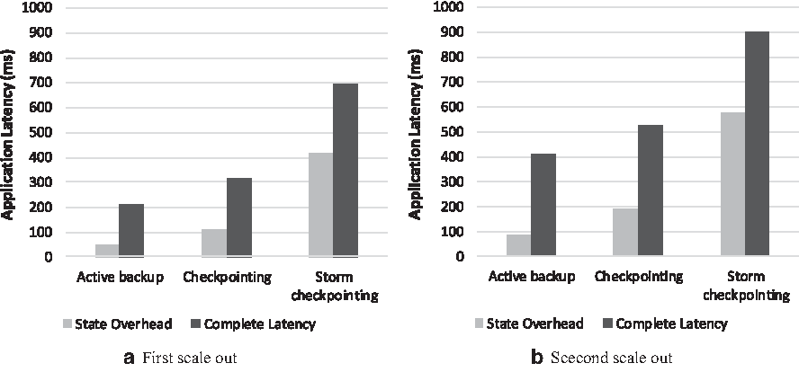
To explore state management overhead, we run the application continuously for 30 minutes by alternating low input rates and high input rates after every 5 minutes and calculated the latency occurred due to state management. Figure 15a and b shows that our techniques are performing better as latency for them is low with respect to Storm's checkpointing mechanism; this is because state checkpointing is performed after every second, which introduces extra overhead and results in more latency. On the contrary, our techniques only store and retrieve state when required, that is, when an operator approaches bottleneck.

OPEN IN VIEWER

FIG. 15.

(a, b) State management overhead.