Abnormal Data Region Discrimination and Cross-Monitoring Points Historical Correlation Repair of Water Intake Data

Introduction

In recent years, with the development of information technology and artificial intelligence technology, China has put forward higher requirements for water resource management, water resource data monitoring, and information statistics. In 2014, Yang and colleagues of Tsinghua University put forward the concept of “Smart Water Affairs,” ¹ and the intelligent water resource monitoring began to be integrated into the development strategy of the “Smart City” and “Digital China.”

For smart water affairs, the acquisition and the processing of the water resource monitoring data (WRMD) are foundational. WRMD belongs to the category of big data. Although big data technologies and methods have been widely studied in the fields of Internet, telecommunications, finance, transportation, medicine, and energy, their research in the field of water resources is still in the initial stage.

Monitoring the daily water intake of water users is an important part of the national water resources data monitoring. But in the actual monitoring and acquisition process, due to the instability of the monitoring environment, monitoring equipment failure, and other factors, the abnormal values, also known as outliers, appear frequently in the monitoring data. These abnormal values always include abnormal large values and value of 0, the existence of which do not conform to the statistical characteristics of the monitoring data, and have a negative impact on the data statistics and analysis, and may lead to wrong statistical results, seriously affecting the accurate information acquisition and reasonable regulation and control measures taken for water resources administration departments.

Meanwhile because of the large sample size of the uploaded data, the manual workload of discriminating and repairing the abnormal and missing data is huge, and it is easy to be neglected or misjudged for the abnormal values. Therefore, it is necessary to study the distinguishing and repairing methods of abnormal data according to the characteristics of the raw monitoring data of daily water intake.

Scholars have done a lot of research on detection and repair of outliers. ² Kriegel et al. ³ unified the exception values provided by various abnormity models and converted any “exception factor” to [0, 1], and the outliers were detected under this conception. She and Owen ⁴ proposed a nonconvex penalty regression outlier discrimination method. The proposed method studies the detection problem of outliers from the view of punitive regression. By improving the regression model, the threshold is introduced in the iterative process of abnormal value detection to realize the rapid determination of the abnormal values.

Lei et al. ⁵ proposed an automatic K-means algorithm for outlier detection. This method includes two stages: clustering and finding outliers. Schubert et al. ⁶ proposed a formal analysis method to the local outlier problem, which is used to compare and popularize many existing methods. Souza et al. ⁷ developed a big data outlier detection program to detect the outliers based on the architecture of Internet of Things, in which K-means algorithm, Hadoop platform, and Mahout algorithm library are used.

Wu and Wang ⁸ proposed an anomaly detection optimization model according to the concept of entropy and all-related holographic entropy. Based on this model, two practical single-parameter anomaly detection methods, information-theory-based step-by-step and information-theory-based single-pass, are proposed. Fabrizio Angiulli ⁹ proposed an anomaly value concept that is named as Concentration Free Outlier Factor (CFOF). Based on this concept, a fast CFOF detection algorithm was proposed to detect abnormal values of very large high-dimensional data sets.

Zimek et al.^10–12 had made deep researches about outlier ensemble detection. Zimek et al. ¹⁰ focus on the core elements of the outliers set, which can provide the model foundation for subsequent research. In Zimek et al., ¹¹ an ensemble detection method based on subsampling technique is proposed. The sample-based anomaly detector was used to improve the results of the same outlier detector on the full data set. In Zimek et al., ¹² an integrated outlier detection algorithm based on active data perturbation was proposed. Zou et al. ¹³ proposed a sparse adaptive compression sampling and online recovery data acquisition (DAF_CSOR) algorithm. Singh et al. ¹⁴ proposed an efficient and fast data recovery algorithm for wireless sensor networks based on orthogonal matching pursuit algorithm.

Most of the mentioned studies can provide basic or prospective theoretical guidance for the identification and restoration of outliers for the field of water resources. Focusing on the field of water resources, the research results of abnormal data discrimination and restoration methods are relatively few, mostly referring to the research and application in other fields. Because of the different characteristics of the data in different fields or the different data structures in the same field, the algorithms proposed are of high pertinence.

Based on the high-dimensional features of the data, Carreira-Perpinan and Lu ¹⁵ applied the globally convergent Gauss–Newton algorithm to optimize the missing data for the high-dimensional data with missing values, and achieved the goal of nonlinear low-dimensional representation and reconstruction of high-dimensional data for the learning data. Jiang et al. ¹⁶ proposed a new regularization method based on tracking norm of robust out-of-sample data recovery model for low-rank restoration of high-dimensional noisy data and applied it to image classification.

Kriegel et al. ¹⁷ proposed an angle-based outlier detection method to evaluate the angle variance between the different vectors of the special fixed point and the other points. Kriegel et al. proposed an original outlier detection mode ¹⁸ to detect outliers in different subspaces of the high-dimensional feature space. According to the experiment results, subspace outlier detection is better than the existing full dimension method, and is suitable for high-dimensional database.

Angiulli and Pizzuti ¹⁹ defined an integer K, and defined the weight of a point as the sum of the distance from the nearest K neighbors, and then proposed a HilOut anomaly detection algorithm, which realizes the effective detection of the former n anomaly values of large- and high-dimensional data sets. Radovanovic et al. ²⁰ proposed a concept of re-examined reverse nearest neighbors in an unsupervised anomaly detection environment, and designed an anomaly detection method based on the angle technology for high-dimensional data.

Based on the clustering features of the data, Song et al. ²¹ proposed a new clustering and repair algorithm in light of the minimum variation principle. They purpose to find the minimum modification of imprecise points, so that the clustering of a large amount of useless data can be enhanced, thereby improving the utilization rate of data.

Based on the sequence characteristics of the data, Zhang et al. ²² proposed a new iterative minimum repair algorithm based on time series data to solve the problem of outliers in time series data. The convergence of the algorithm was analyzed and the parameters were effectively estimated. Song et al. proposed a flow data repair method based on SCREEN first constraint by Song et al. ²³ The data sequence is repaired as a whole, and an adaptive window size is used to balance the repairing accuracy and efficiency.

Based on the functional characteristics of data, Volkovs et al. ²⁴ proposed a continuous data restoration method that can be applied to dynamic data and constrained environments. The proposed method not only uses data and constraints as evidence, but also considers predicting the changes of repair types according to historical repair methods to recommend a more accurate repair strategy.

Although the mentioned methods are widely used in specific fields, they are not suitable for solving the problem of abnormal values in this article because of the diversity and specificity of the outlier problems in various fields, which are mainly reflected in the following aspects: (1) the abnormal data of this article are not only related with data value, but also with the neighborhood distribution, whereas most of proposed methods detect abnormal value just according to data value or its global statistic property; therefore, these methods are not ideal for neighborhood-related abnormal data; (2) most proposed methods use historical distribution of data set to estimate abnormal value, but for our problem, the data distribution of each node does not strictly conform to the historical data, thus the best estimation cannot be obtained just from current node's history record; (3) prior knowledge of the data sets reflected in the existing algorithms is insufficient, so most of the algorithms realized the discrimination by Euclidean distance between the data. Therefore the above algorithms can not be used to distinguish and repair abnormal values in the data of daily water intake because of the specificity of the data characteristics.

However, the research ideas and methods embodied in the mentioned research provide important reference for the study of abnormal value discrimination and repair of water intake data. On the premise of fully recognizing the characteristics of the data, this article comprehensively analyzed the internal and external environment of the data generation, and proposed a pertinent discrimination and repair algorithm.

Based on this, the monitoring of water intake data was preliminarily observed, and the preliminary tests were taken, by which it was found that the water intake data have the characteristics of space, time series, and function. Therefore, on the foundation of analyzing the characteristics of the abnormal data of daily water intake, and referring to the research ideas and methods of abnormal data discrimination and repair according to the spatial, time series, and function features in the mentioned results, this article puts forward an abnormal data region discrimination (ADRD) algorithm, and proposed a method of cross-monitoring points historical correlation repair (CMHCR) according to the correlation of data between monitoring points (MPs).

The remainder of this article is organized as follows. In the Abnormal Value Analysis of Water Intake Data section, we analyze the characteristics of abnormal value of water intake. The algorithm for ADRD is proposed in the ADRD Algorithm section, a method proposed for CMHCR is described in the CMHCR Method section, the experiments performed and the results are analyzed in the Experimental Results and Analysis section, and concluding remarks are presented in the Conclusion section.

Abnormal Value Analysis of Water Intake Data

Analysis of abnormal values of water intake data

According to the preliminary analysis results of monitoring data, the monitoring data anomalies of water stations are mainly abnormal high-value points, that is, the data of the first few days are 0, and the monitoring data of the next day is abnormally large, the reason for the abnormal large value may be the sum of the actual daily water intake values of the previous few days.

Figure 1 shows the data trend of the daily water intake from MP 1 of a water station in Guangdong in February 2017. As can be seen from Figure 1, the water intake data in this MP appeared an obvious anomaly on February 9. If the data set is \documentclass{aastex}\usepackage{amsbsy}\usepackage{amsfonts}\usepackage{amssymb}\usepackage{bm}\usepackage{mathrsfs}\usepackage{pifont}\usepackage{stmaryrd}\usepackage{textcomp}\usepackage{portland, xspace}\usepackage{amsmath, amsxtra}\usepackage{upgreek}\pagestyle{empty}\DeclareMathSizes{10}{9}{7}{6}\begin{document} $${S \prime _2}$$ \end{document} , then \documentclass{aastex}\usepackage{amsbsy}\usepackage{amsfonts}\usepackage{amssymb}\usepackage{bm}\usepackage{mathrsfs}\usepackage{pifont}\usepackage{stmaryrd}\usepackage{textcomp}\usepackage{portland, xspace}\usepackage{amsmath, amsxtra}\usepackage{upgreek}\pagestyle{empty}\DeclareMathSizes{10}{9}{7}{6}\begin{document} $$E ( {S \prime _2} ) = 3390.8$$ \end{document} , \documentclass{aastex}\usepackage{amsbsy}\usepackage{amsfonts}\usepackage{amssymb}\usepackage{bm}\usepackage{mathrsfs}\usepackage{pifont}\usepackage{stmaryrd}\usepackage{textcomp}\usepackage{portland, xspace}\usepackage{amsmath, amsxtra}\usepackage{upgreek}\pagestyle{empty}\DeclareMathSizes{10}{9}{7}{6}\begin{document} $${s \prime _{29}} = 25730$$ \end{document} , the ratio of the two is:

\documentclass{aastex}\usepackage{amsbsy}\usepackage{amsfonts}\usepackage{amssymb}\usepackage{bm}\usepackage{mathrsfs}\usepackage{pifont}\usepackage{stmaryrd}\usepackage{textcomp}\usepackage{portland, xspace}\usepackage{amsmath, amsxtra}\usepackage{upgreek}\pagestyle{empty}\DeclareMathSizes{10}{9}{7}{6}\begin{document} \begin{align*} { K_ { { { s \prime } _ { 29 } } } } = { \frac { { { s \prime } _ { 29 } } } { E ( { { S \prime } _2 } ) } } = 7.6. \tag { 2 } \end{align*} \end{document} OPEN IN VIEWER

FIG. 1.

Water intake data trend for MP 1 in February 2017. MP, monitoring point.

That is, the data of February 9 is 7.6 times of the average. According to the trend of the curve, the data on February 9 is actually the sum of the data of the 6 days from February 4 to February 9. The characteristics of this kind of abnormal data are obvious.

Compared with other data, abnormal data can be found to have the same law. Based on the mentioned analysis, the characteristics of the abnormal data can be defined. Setting \documentclass{aastex}\usepackage{amsbsy}\usepackage{amsfonts}\usepackage{amssymb}\usepackage{bm}\usepackage{mathrsfs}\usepackage{pifont}\usepackage{stmaryrd}\usepackage{textcomp}\usepackage{portland, xspace}\usepackage{amsmath, amsxtra}\usepackage{upgreek}\pagestyle{empty}\DeclareMathSizes{10}{9}{7}{6}\begin{document} $${S \prime \prime _2}$$ \end{document} as subset of abnormal data area, then \documentclass{aastex}\usepackage{amsbsy}\usepackage{amsfonts}\usepackage{amssymb}\usepackage{bm}\usepackage{mathrsfs}\usepackage{pifont}\usepackage{stmaryrd}\usepackage{textcomp}\usepackage{portland, xspace}\usepackage{amsmath, amsxtra}\usepackage{upgreek}\pagestyle{empty}\DeclareMathSizes{10}{9}{7}{6}\begin{document} $${S \prime \prime _2} \subset {S \prime _2}$$ \end{document} , and \documentclass{aastex}\usepackage{amsbsy}\usepackage{amsfonts}\usepackage{amssymb}\usepackage{bm}\usepackage{mathrsfs}\usepackage{pifont}\usepackage{stmaryrd}\usepackage{textcomp}\usepackage{portland, xspace}\usepackage{amsmath, amsxtra}\usepackage{upgreek}\pagestyle{empty}\DeclareMathSizes{10}{9}{7}{6}\begin{document} $${S \prime \prime _2} \subset {S \prime _2}$$ \end{document} , and elements in \documentclass{aastex}\usepackage{amsbsy}\usepackage{amsfonts}\usepackage{amssymb}\usepackage{bm}\usepackage{mathrsfs}\usepackage{pifont}\usepackage{stmaryrd}\usepackage{textcomp}\usepackage{portland, xspace}\usepackage{amsmath, amsxtra}\usepackage{upgreek}\pagestyle{empty}\DeclareMathSizes{10}{9}{7}{6}\begin{document} $${S \prime \prime _2}$$ \end{document} are outliers.

(1)

There must be one or more 0 value points in front of the abnormal data.

(2)

The abnormal data are the expected multiples of the data, which is close to the missing days.

Therefore, according to the characteristics of the data, the location of the abnormal data can be identified by 0 value discrimination instead of using \documentclass{aastex}\usepackage{amsbsy}\usepackage{amsfonts}\usepackage{amssymb}\usepackage{bm}\usepackage{mathrsfs}\usepackage{pifont}\usepackage{stmaryrd}\usepackage{textcomp}\usepackage{portland, xspace}\usepackage{amsmath, amsxtra}\usepackage{upgreek}\pagestyle{empty}\DeclareMathSizes{10}{9}{7}{6}\begin{document} $$3 \sigma$$ \end{document} criteria, which not only improves the efficiency but also lays a foundation for abnormal data real-time identification and reparation.

ADRD Algorithm

According to the rule of abnormal data, the abnormal data can be positioned by 0 value discrimination, but when the monitoring data are 0, they are not necessarily abnormal data. Therefore, it is necessary to study the abnormal data positioning algorithm through the rule of abnormal data.

Setting \documentclass{aastex}\usepackage{amsbsy}\usepackage{amsfonts}\usepackage{amssymb}\usepackage{bm}\usepackage{mathrsfs}\usepackage{pifont}\usepackage{stmaryrd}\usepackage{textcomp}\usepackage{portland, xspace}\usepackage{amsmath, amsxtra}\usepackage{upgreek}\pagestyle{empty}\DeclareMathSizes{10}{9}{7}{6}\begin{document} $${s\prime _i}$$ \end{document} is abnormal data, before \documentclass{aastex}\usepackage{amsbsy}\usepackage{amsfonts}\usepackage{amssymb}\usepackage{bm}\usepackage{mathrsfs}\usepackage{pifont}\usepackage{stmaryrd}\usepackage{textcomp}\usepackage{portland, xspace}\usepackage{amsmath, amsxtra}\usepackage{upgreek}\pagestyle{empty}\DeclareMathSizes{10}{9}{7}{6}\begin{document} $${s\prime _i}$$ \end{document} , there is K 0 value data, and then the subset of the abnormal data is \documentclass{aastex}\usepackage{amsbsy}\usepackage{amsfonts}\usepackage{amssymb}\usepackage{bm}\usepackage{mathrsfs}\usepackage{pifont}\usepackage{stmaryrd}\usepackage{textcomp}\usepackage{portland, xspace}\usepackage{amsmath, amsxtra}\usepackage{upgreek}\pagestyle{empty}\DeclareMathSizes{10}{9}{7}{6}\begin{document} \begin{align*} \begin{split} & {{S \prime }_Y} = \{ {{s \prime } _{i - k}} , {{s \prime }_{i - k + 1}} , \cdots , {{s \prime } _{i - 1}} , {{s \prime } _i} \} \\ & s.t:{{s \prime } _j} = 0 , j = i - k , i - k + 1 , \cdots , i - 1 \end{split} . \tag{3} \end{align*} \end{document}

Inference 1: If \documentclass{aastex}\usepackage{amsbsy}\usepackage{amsfonts}\usepackage{amssymb}\usepackage{bm}\usepackage{mathrsfs}\usepackage{pifont}\usepackage{stmaryrd}\usepackage{textcomp}\usepackage{portland, xspace}\usepackage{amsmath, amsxtra}\usepackage{upgreek}\pagestyle{empty}\DeclareMathSizes{10}{9}{7}{6}\begin{document} $${s\prime _i}$$ \end{document} is the abnormal maximum value in the measuring node, there must be 0 value points in \documentclass{aastex}\usepackage{amsbsy}\usepackage{amsfonts}\usepackage{amssymb}\usepackage{bm}\usepackage{mathrsfs}\usepackage{pifont}\usepackage{stmaryrd}\usepackage{textcomp}\usepackage{portland, xspace}\usepackage{amsmath, amsxtra}\usepackage{upgreek}\pagestyle{empty}\DeclareMathSizes{10}{9}{7}{6}\begin{document} $${S \prime _Y}$$ \end{document} .

Inference 2: If there is a 0 point before \documentclass{aastex}\usepackage{amsbsy}\usepackage{amsfonts}\usepackage{amssymb}\usepackage{bm}\usepackage{mathrsfs}\usepackage{pifont}\usepackage{stmaryrd}\usepackage{textcomp}\usepackage{portland, xspace}\usepackage{amsmath, amsxtra}\usepackage{upgreek}\pagestyle{empty}\DeclareMathSizes{10}{9}{7}{6}\begin{document} $${s\prime _i}$$ \end{document} , the necessary condition for \documentclass{aastex}\usepackage{amsbsy}\usepackage{amsfonts}\usepackage{amssymb}\usepackage{bm}\usepackage{mathrsfs}\usepackage{pifont}\usepackage{stmaryrd}\usepackage{textcomp}\usepackage{portland, xspace}\usepackage{amsmath, amsxtra}\usepackage{upgreek}\pagestyle{empty}\DeclareMathSizes{10}{9}{7}{6}\begin{document} $${s\prime _i}$$ \end{document} being an abnormal data point is that there is a significant difference between the expected value of the normal data set and \documentclass{aastex}\usepackage{amsbsy}\usepackage{amsfonts}\usepackage{amssymb}\usepackage{bm}\usepackage{mathrsfs}\usepackage{pifont}\usepackage{stmaryrd}\usepackage{textcomp}\usepackage{portland, xspace}\usepackage{amsmath, amsxtra}\usepackage{upgreek}\pagestyle{empty}\DeclareMathSizes{10}{9}{7}{6}\begin{document} $${s\prime _i}$$ \end{document} .

According to inference 2, if there is a 0 point before the data \documentclass{aastex}\usepackage{amsbsy}\usepackage{amsfonts}\usepackage{amssymb}\usepackage{bm}\usepackage{mathrsfs}\usepackage{pifont}\usepackage{stmaryrd}\usepackage{textcomp}\usepackage{portland, xspace}\usepackage{amsmath, amsxtra}\usepackage{upgreek}\pagestyle{empty}\DeclareMathSizes{10}{9}{7}{6}\begin{document} $${s\prime _i}$$ \end{document} , but the value of \documentclass{aastex}\usepackage{amsbsy}\usepackage{amsfonts}\usepackage{amssymb}\usepackage{bm}\usepackage{mathrsfs}\usepackage{pifont}\usepackage{stmaryrd}\usepackage{textcomp}\usepackage{portland, xspace}\usepackage{amsmath, amsxtra}\usepackage{upgreek}\pagestyle{empty}\DeclareMathSizes{10}{9}{7}{6}\begin{document} $${s\prime _i}$$ \end{document} is close to the expectation of the whole data set, it should be ruled out. The 0 point is generated by normal work.

According to the mentioned discussion, the key to distinguish abnormal data is the difference degree between the expected value of normal data set and the value of the abnormal data set. According to the generation rule of abnormal value, the more the 0 points before the abnormal value, the bigger the value of abnormal data, and the abnormal region is easier to distinguish. When there is only one 0 point in front, it is easy to confuse the normal value with the abnormal value \documentclass{aastex}\usepackage{amsbsy}\usepackage{amsfonts}\usepackage{amssymb}\usepackage{bm}\usepackage{mathrsfs}\usepackage{pifont}\usepackage{stmaryrd}\usepackage{textcomp}\usepackage{portland, xspace}\usepackage{amsmath, amsxtra}\usepackage{upgreek}\pagestyle{empty}\DeclareMathSizes{10}{9}{7}{6}\begin{document} $${s\prime _i}$$ \end{document} . Therefore, the discrimination of single 0 point outliers becomes the key to distinguish.

Assuming the ideal monitoring data set is \documentclass{aastex}\usepackage{amsbsy}\usepackage{amsfonts}\usepackage{amssymb}\usepackage{bm}\usepackage{mathrsfs}\usepackage{pifont}\usepackage{stmaryrd}\usepackage{textcomp}\usepackage{portland, xspace}\usepackage{amsmath, amsxtra}\usepackage{upgreek}\pagestyle{empty}\DeclareMathSizes{10}{9}{7}{6}\begin{document} $${S \prime _I}$$ \end{document} , its elements contain the following characteristics:

According to the mentioned characteristics of \documentclass{aastex}\usepackage{amsbsy}\usepackage{amsfonts}\usepackage{amssymb}\usepackage{bm}\usepackage{mathrsfs}\usepackage{pifont}\usepackage{stmaryrd}\usepackage{textcomp}\usepackage{portland, xspace}\usepackage{amsmath, amsxtra}\usepackage{upgreek}\pagestyle{empty}\DeclareMathSizes{10}{9}{7}{6}\begin{document} $${S \prime _I}$$ \end{document} , when \documentclass{aastex}\usepackage{amsbsy}\usepackage{amsfonts}\usepackage{amssymb}\usepackage{bm}\usepackage{mathrsfs}\usepackage{pifont}\usepackage{stmaryrd}\usepackage{textcomp}\usepackage{portland, xspace}\usepackage{amsmath, amsxtra}\usepackage{upgreek}\pagestyle{empty}\DeclareMathSizes{10}{9}{7}{6}\begin{document} $${s \prime _{Ii}}$$ \end{document} is an abnormal data, the ratio of \documentclass{aastex}\usepackage{amsbsy}\usepackage{amsfonts}\usepackage{amssymb}\usepackage{bm}\usepackage{mathrsfs}\usepackage{pifont}\usepackage{stmaryrd}\usepackage{textcomp}\usepackage{portland, xspace}\usepackage{amsmath, amsxtra}\usepackage{upgreek}\pagestyle{empty}\DeclareMathSizes{10}{9}{7}{6}\begin{document} $${s \prime _{Ii}}$$ \end{document} to \documentclass{aastex}\usepackage{amsbsy}\usepackage{amsfonts}\usepackage{amssymb}\usepackage{bm}\usepackage{mathrsfs}\usepackage{pifont}\usepackage{stmaryrd}\usepackage{textcomp}\usepackage{portland, xspace}\usepackage{amsmath, amsxtra}\usepackage{upgreek}\pagestyle{empty}\DeclareMathSizes{10}{9}{7}{6}\begin{document} $$E ( {S \prime _I} )$$ \end{document} satisfies the following conditions: \documentclass{aastex}\usepackage{amsbsy}\usepackage{amsfonts}\usepackage{amssymb}\usepackage{bm}\usepackage{mathrsfs}\usepackage{pifont}\usepackage{stmaryrd}\usepackage{textcomp}\usepackage{portland, xspace}\usepackage{amsmath, amsxtra}\usepackage{upgreek}\pagestyle{empty}\DeclareMathSizes{10}{9}{7}{6}\begin{document} \begin{align*} { K_ { { { s \prime } _ { Ii } } } } = { \frac { { { s \prime } _ { Ii } } } { E ( { { S \prime } _I } ) } } = k + 1. \tag { 4 } \end{align*} \end{document}

Here k is the number of 0 value points in front of \documentclass{aastex}\usepackage{amsbsy}\usepackage{amsfonts}\usepackage{amssymb}\usepackage{bm}\usepackage{mathrsfs}\usepackage{pifont}\usepackage{stmaryrd}\usepackage{textcomp}\usepackage{portland, xspace}\usepackage{amsmath, amsxtra}\usepackage{upgreek}\pagestyle{empty}\DeclareMathSizes{10}{9}{7}{6}\begin{document} $${s \prime _{Ii}}$$ \end{document} , so the minimum value of \documentclass{aastex}\usepackage{amsbsy}\usepackage{amsfonts}\usepackage{amssymb}\usepackage{bm}\usepackage{mathrsfs}\usepackage{pifont}\usepackage{stmaryrd}\usepackage{textcomp}\usepackage{portland, xspace}\usepackage{amsmath, amsxtra}\usepackage{upgreek}\pagestyle{empty}\DeclareMathSizes{10}{9}{7}{6}\begin{document} $${K_{{{s \prime } _{Ii}}}}$$ \end{document} is 2. Therefore, the discriminant condition for abnormal data \documentclass{aastex}\usepackage{amsbsy}\usepackage{amsfonts}\usepackage{amssymb}\usepackage{bm}\usepackage{mathrsfs}\usepackage{pifont}\usepackage{stmaryrd}\usepackage{textcomp}\usepackage{portland, xspace}\usepackage{amsmath, amsxtra}\usepackage{upgreek}\pagestyle{empty}\DeclareMathSizes{10}{9}{7}{6}\begin{document} $${S \prime _I}$$ \end{document} is \documentclass{aastex}\usepackage{amsbsy}\usepackage{amsfonts}\usepackage{amssymb}\usepackage{bm}\usepackage{mathrsfs}\usepackage{pifont}\usepackage{stmaryrd}\usepackage{textcomp}\usepackage{portland, xspace}\usepackage{amsmath, amsxtra}\usepackage{upgreek}\pagestyle{empty}\DeclareMathSizes{10}{9}{7}{6}\begin{document} $${K_{{{s \prime } _{Ii}}}} \ge 2$$ \end{document} .

In the actual data set, because the water intake changes with time, the abnormal data \documentclass{aastex}\usepackage{amsbsy}\usepackage{amsfonts}\usepackage{amssymb}\usepackage{bm}\usepackage{mathrsfs}\usepackage{pifont}\usepackage{stmaryrd}\usepackage{textcomp}\usepackage{portland, xspace}\usepackage{amsmath, amsxtra}\usepackage{upgreek}\pagestyle{empty}\DeclareMathSizes{10}{9}{7}{6}\begin{document} $${K_{{{s \prime } _i}}}$$ \end{document} must be >1, but its minimum value may be <2. According to the changing law of the data, combined with the mentioned general trend, it can be defined that \documentclass{aastex}\usepackage{amsbsy}\usepackage{amsfonts}\usepackage{amssymb}\usepackage{bm}\usepackage{mathrsfs}\usepackage{pifont}\usepackage{stmaryrd}\usepackage{textcomp}\usepackage{portland, xspace}\usepackage{amsmath, amsxtra}\usepackage{upgreek}\pagestyle{empty}\DeclareMathSizes{10}{9}{7}{6}\begin{document} $${K_{ \min }} = 2$$ \end{document} .

Based on the mentioned discussion, the discriminant criterion for abnormal data is defined as

Abnormal data discrimination algorithm:

Step 1: \documentclass{aastex}\usepackage{amsbsy}\usepackage{amsfonts}\usepackage{amssymb}\usepackage{bm}\usepackage{mathrsfs}\usepackage{pifont}\usepackage{stmaryrd}\usepackage{textcomp}\usepackage{portland, xspace}\usepackage{amsmath, amsxtra}\usepackage{upgreek}\pagestyle{empty}\DeclareMathSizes{10}{9}{7}{6}\begin{document} $$k = 0$$ \end{document} , \documentclass{aastex}\usepackage{amsbsy}\usepackage{amsfonts}\usepackage{amssymb}\usepackage{bm}\usepackage{mathrsfs}\usepackage{pifont}\usepackage{stmaryrd}\usepackage{textcomp}\usepackage{portland, xspace}\usepackage{amsmath, amsxtra}\usepackage{upgreek}\pagestyle{empty}\DeclareMathSizes{10}{9}{7}{6}\begin{document} $$j = 1$$ \end{document} , and \documentclass{aastex}\usepackage{amsbsy}\usepackage{amsfonts}\usepackage{amssymb}\usepackage{bm}\usepackage{mathrsfs}\usepackage{pifont}\usepackage{stmaryrd}\usepackage{textcomp}\usepackage{portland, xspace}\usepackage{amsmath, amsxtra}\usepackage{upgreek}\pagestyle{empty}\DeclareMathSizes{10}{9}{7}{6}\begin{document} $${K_{ \min }} = 2$$ \end{document} ;

Step 2: Discriminate data \documentclass{aastex}\usepackage{amsbsy}\usepackage{amsfonts}\usepackage{amssymb}\usepackage{bm}\usepackage{mathrsfs}\usepackage{pifont}\usepackage{stmaryrd}\usepackage{textcomp}\usepackage{portland, xspace}\usepackage{amsmath, amsxtra}\usepackage{upgreek}\pagestyle{empty}\DeclareMathSizes{10}{9}{7}{6}\begin{document} $${s \prime _j}$$ \end{document} . If \documentclass{aastex}\usepackage{amsbsy}\usepackage{amsfonts}\usepackage{amssymb}\usepackage{bm}\usepackage{mathrsfs}\usepackage{pifont}\usepackage{stmaryrd}\usepackage{textcomp}\usepackage{portland, xspace}\usepackage{amsmath, amsxtra}\usepackage{upgreek}\pagestyle{empty}\DeclareMathSizes{10}{9}{7}{6}\begin{document} $${s \prime _j} = 0$$ \end{document} , Step 3 is implemented, otherwise \documentclass{aastex}\usepackage{amsbsy}\usepackage{amsfonts}\usepackage{amssymb}\usepackage{bm}\usepackage{mathrsfs}\usepackage{pifont}\usepackage{stmaryrd}\usepackage{textcomp}\usepackage{portland, xspace}\usepackage{amsmath, amsxtra}\usepackage{upgreek}\pagestyle{empty}\DeclareMathSizes{10}{9}{7}{6}\begin{document} $$j = j + 1$$ \end{document} . Discrimination completion condition: if \documentclass{aastex}\usepackage{amsbsy}\usepackage{amsfonts}\usepackage{amssymb}\usepackage{bm}\usepackage{mathrsfs}\usepackage{pifont}\usepackage{stmaryrd}\usepackage{textcomp}\usepackage{portland, xspace}\usepackage{amsmath, amsxtra}\usepackage{upgreek}\pagestyle{empty}\DeclareMathSizes{10}{9}{7}{6}\begin{document} $$j > n$$ \end{document} , complete the discrimination, otherwise repeat Step 2;

Step 3: Mark data \documentclass{aastex}\usepackage{amsbsy}\usepackage{amsfonts}\usepackage{amssymb}\usepackage{bm}\usepackage{mathrsfs}\usepackage{pifont}\usepackage{stmaryrd}\usepackage{textcomp}\usepackage{portland, xspace}\usepackage{amsmath, amsxtra}\usepackage{upgreek}\pagestyle{empty}\DeclareMathSizes{10}{9}{7}{6}\begin{document} $${s \prime _j}$$ \end{document} . \documentclass{aastex}\usepackage{amsbsy}\usepackage{amsfonts}\usepackage{amssymb}\usepackage{bm}\usepackage{mathrsfs}\usepackage{pifont}\usepackage{stmaryrd}\usepackage{textcomp}\usepackage{portland, xspace}\usepackage{amsmath, amsxtra}\usepackage{upgreek}\pagestyle{empty}\DeclareMathSizes{10}{9}{7}{6}\begin{document} $$k = k + 1$$ \end{document} , \documentclass{aastex}\usepackage{amsbsy}\usepackage{amsfonts}\usepackage{amssymb}\usepackage{bm}\usepackage{mathrsfs}\usepackage{pifont}\usepackage{stmaryrd}\usepackage{textcomp}\usepackage{portland, xspace}\usepackage{amsmath, amsxtra}\usepackage{upgreek}\pagestyle{empty}\DeclareMathSizes{10}{9}{7}{6}\begin{document} $$j = j + 1$$ \end{document} . Distinguish \documentclass{aastex}\usepackage{amsbsy}\usepackage{amsfonts}\usepackage{amssymb}\usepackage{bm}\usepackage{mathrsfs}\usepackage{pifont}\usepackage{stmaryrd}\usepackage{textcomp}\usepackage{portland, xspace}\usepackage{amsmath, amsxtra}\usepackage{upgreek}\pagestyle{empty}\DeclareMathSizes{10}{9}{7}{6}\begin{document} $${s \prime _j}$$ \end{document} . If \documentclass{aastex}\usepackage{amsbsy}\usepackage{amsfonts}\usepackage{amssymb}\usepackage{bm}\usepackage{mathrsfs}\usepackage{pifont}\usepackage{stmaryrd}\usepackage{textcomp}\usepackage{portland, xspace}\usepackage{amsmath, amsxtra}\usepackage{upgreek}\pagestyle{empty}\DeclareMathSizes{10}{9}{7}{6}\begin{document} $${s \prime _j} = 0$$ \end{document} , repeat Step 3, otherwise continue;

Step 4: Compute \documentclass{aastex}\usepackage{amsbsy}\usepackage{amsfonts}\usepackage{amssymb}\usepackage{bm}\usepackage{mathrsfs}\usepackage{pifont}\usepackage{stmaryrd}\usepackage{textcomp}\usepackage{portland, xspace}\usepackage{amsmath, amsxtra}\usepackage{upgreek}\pagestyle{empty}\DeclareMathSizes{10}{9}{7}{6}\begin{document} $${K_{{{s \prime } _j}}}$$ \end{document} . If \documentclass{aastex}\usepackage{amsbsy}\usepackage{amsfonts}\usepackage{amssymb}\usepackage{bm}\usepackage{mathrsfs}\usepackage{pifont}\usepackage{stmaryrd}\usepackage{textcomp}\usepackage{portland, xspace}\usepackage{amsmath, amsxtra}\usepackage{upgreek}\pagestyle{empty}\DeclareMathSizes{10}{9}{7}{6}\begin{document} $${K_{{{s \prime } _j}}} \ge {K_{ \min }}$$ \end{document} , then mark \documentclass{aastex}\usepackage{amsbsy}\usepackage{amsfonts}\usepackage{amssymb}\usepackage{bm}\usepackage{mathrsfs}\usepackage{pifont}\usepackage{stmaryrd}\usepackage{textcomp}\usepackage{portland, xspace}\usepackage{amsmath, amsxtra}\usepackage{upgreek}\pagestyle{empty}\DeclareMathSizes{10}{9}{7}{6}\begin{document} $${s \prime _j}$$ \end{document} as an abnormal data point, build a subset of abnormal data \documentclass{aastex}\usepackage{amsbsy}\usepackage{amsfonts}\usepackage{amssymb}\usepackage{bm}\usepackage{mathrsfs}\usepackage{pifont}\usepackage{stmaryrd}\usepackage{textcomp}\usepackage{portland, xspace}\usepackage{amsmath, amsxtra}\usepackage{upgreek}\pagestyle{empty}\DeclareMathSizes{10}{9}{7}{6}\begin{document} $${S \prime _Y} = \{ {s \prime _{i - k}} , {s \prime _{i - k + 1}} , \cdots , {s \prime _{i - 1}} , {s\prime _i} \} $$ \end{document} , and record k, or continue;

Step 5: \documentclass{aastex}\usepackage{amsbsy}\usepackage{amsfonts}\usepackage{amssymb}\usepackage{bm}\usepackage{mathrsfs}\usepackage{pifont}\usepackage{stmaryrd}\usepackage{textcomp}\usepackage{portland, xspace}\usepackage{amsmath, amsxtra}\usepackage{upgreek}\pagestyle{empty}\DeclareMathSizes{10}{9}{7}{6}\begin{document} $$k = 0$$ \end{document} , \documentclass{aastex}\usepackage{amsbsy}\usepackage{amsfonts}\usepackage{amssymb}\usepackage{bm}\usepackage{mathrsfs}\usepackage{pifont}\usepackage{stmaryrd}\usepackage{textcomp}\usepackage{portland, xspace}\usepackage{amsmath, amsxtra}\usepackage{upgreek}\pagestyle{empty}\DeclareMathSizes{10}{9}{7}{6}\begin{document} $$j = j + 1$$ \end{document} , and repeat Step 2.

CMHCR Method

In judging the abnormal data, the proposed algorithm can locate the abnormal data accurately and determine the abnormal data region. To get the more accurate rules and trends of the data system, it is necessary to repair the abnormal data region.

The basic idea of repairing abnormal data is to make use of the characteristics of historical data correlation. The corresponding data in March 2016 and 2017 are analyzed, and the comparison curves are shown in Figures 2–7.

OPEN IN VIEWER

FIG. 2.

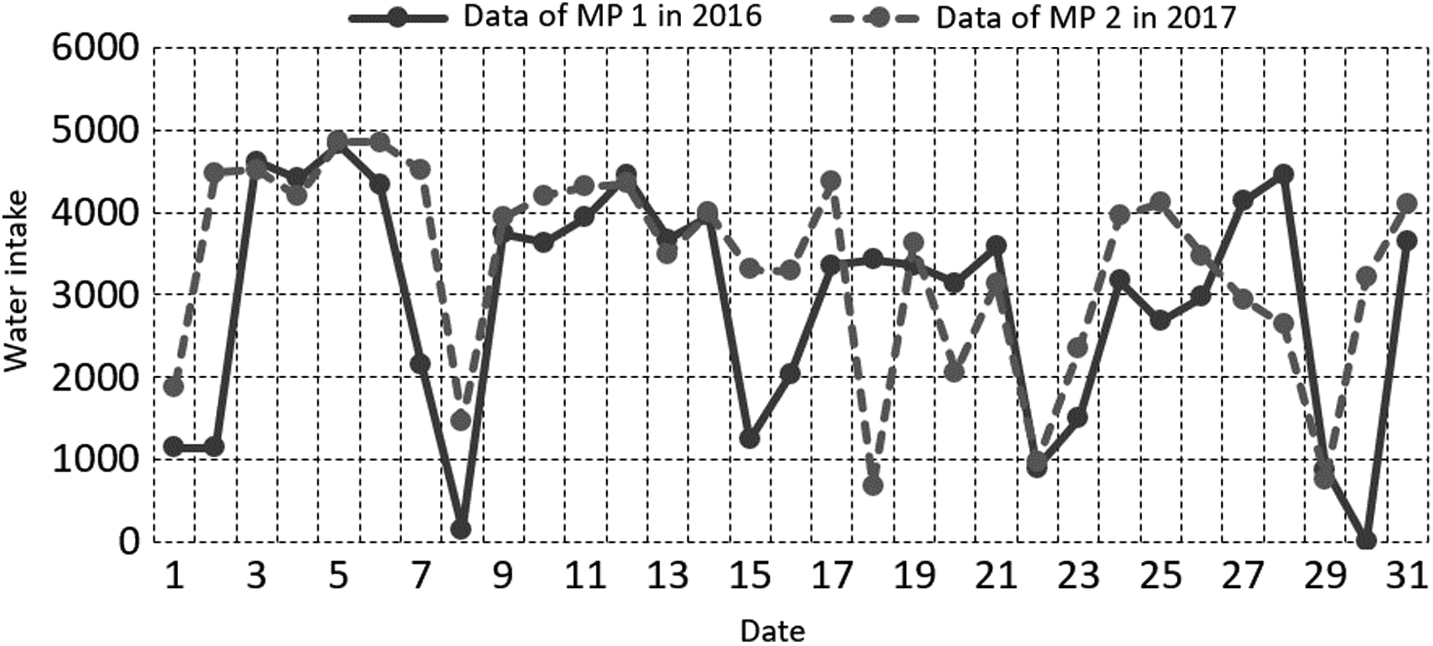
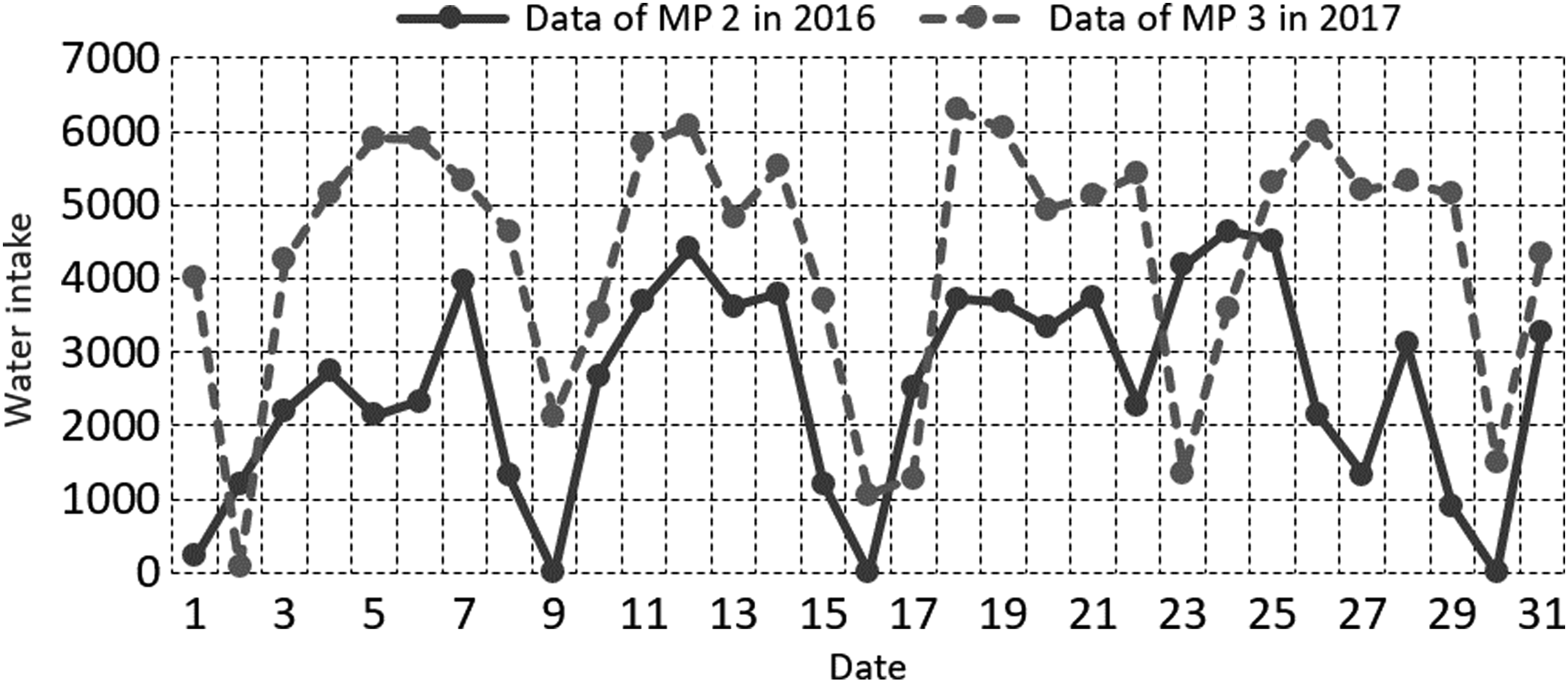
Contrast of water intake between 2016 and 2017 for MP 1.

OPEN IN VIEWER

FIG. 3.

Contrast of water intake between 2016 and 2017 for MP 2.

OPEN IN VIEWER

FIG. 4.

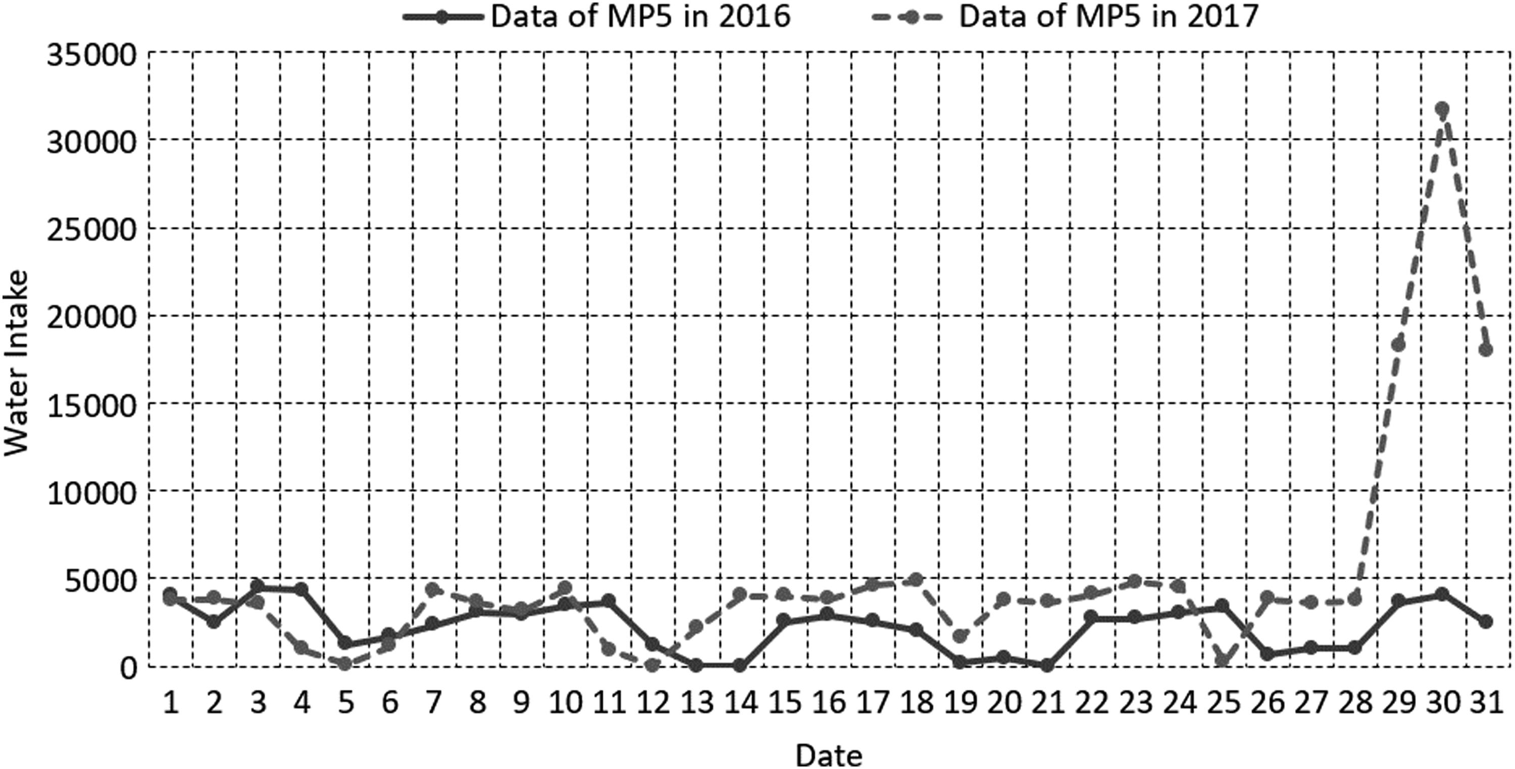
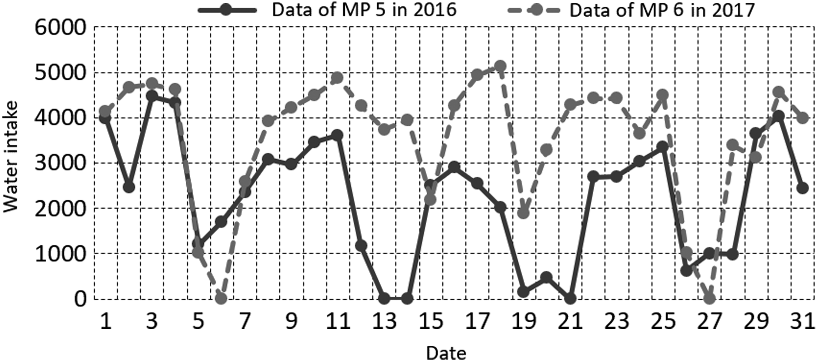
Contrast of water intake between 2016 and 2017 for MP 3.

OPEN IN VIEWER

FIG. 5.

Contrast of water intake between 2016 and 2017 for MP 4.

OPEN IN VIEWER

FIG. 6.

Contrast of water intake between 2016 and 2017 for MP 5.

OPEN IN VIEWER

FIG. 7.

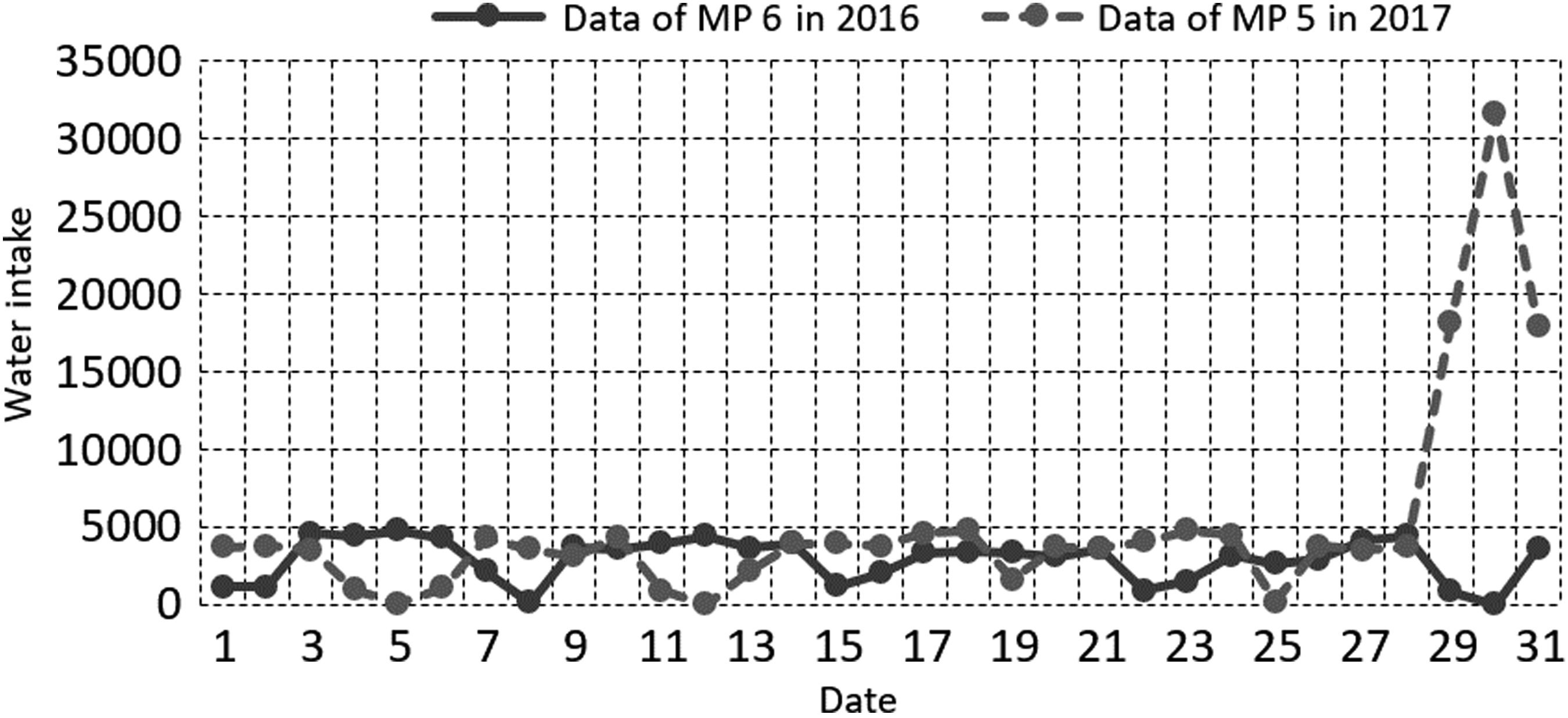
Contrast of water intake between 2016 and 2017 for MP 6.

As can be seen from Figures 2–7, for fixed nodes, the correlation between the 2 years’ water intake data is not obvious, so using the historical data of corresponding nodes to predict the current data will bring a larger deviation. For a certain water intake station, because of the continuity of the water unit, the sums of the water intake are related. As can be seen in Figures 2 to 7, the total water intake in 2 years is basically balanced, so the current data of each measuring point must be related to the corresponding node data in the previous year. Correlation analysis was performed on all node data in 2016 and 2017, and the correlation coefficient is given in Table 1.

According to Table 1, for each current measurement point, there is always a maximum relevant historical measurement point corresponding to it, but the historical measurement point is not necessarily the corresponding node. For a certain measuring point, even if the greatest correlation data with the historical measuring point are far from 1, strictly speaking, the correlation coefficient is not linear. But to repair the abnormal data region, in the case of serious missing statistical information, the maximum correlation data are the closest to the current data distribution, and it is also the best reference value for the statistical characteristics of the repair data, so this article uses the CMHCR method to repair the abnormal data region.

The corresponding water intake curves of the maximum points are compared in Table 1, as is shown in Figures 8–13.

OPEN IN VIEWER

FIG. 8.

Comparison of water intake trend between MP 5 in 2016 and MP 1 in 2017.

OPEN IN VIEWER

FIG. 9.

Comparison of water intake trend between MP 1 in 2016 and MP 2 in 2017.

OPEN IN VIEWER

FIG. 10.

Comparison of water intake trend between MP 2 in 2016 and MP 3 in 2017.

OPEN IN VIEWER

FIG. 11.

Comparison of water intake trend between MP 3 in 2016 and MP 4 in 2017.

OPEN IN VIEWER

FIG. 12.

Comparison of water intake trend between MP 6 in 2016 and MP 5 in 2017.

OPEN IN VIEWER

FIG. 13.

Comparison of water intake trend between MP 5 in 2016 and MP 6 in 2017.

As can be seen from these figures, the regularity of the curve corresponding to the maximum correlation is obviously better than that of the data of measuring points, indicating that the result estimated by the maximum correlated historical data is better than that estimated by the corresponding measuring points.

Based on the mentioned analysis, the following parameters estimation criteria can be obtained.

For the water intake data set with n measuring points, set \documentclass{aastex}\usepackage{amsbsy}\usepackage{amsfonts}\usepackage{amssymb}\usepackage{bm}\usepackage{mathrsfs}\usepackage{pifont}\usepackage{stmaryrd}\usepackage{textcomp}\usepackage{portland, xspace}\usepackage{amsmath, amsxtra}\usepackage{upgreek}\pagestyle{empty}\DeclareMathSizes{10}{9}{7}{6}\begin{document} $${S_{newi}}$$ \end{document} as the current data set corresponding to the measuring point i, and \documentclass{aastex}\usepackage{amsbsy}\usepackage{amsfonts}\usepackage{amssymb}\usepackage{bm}\usepackage{mathrsfs}\usepackage{pifont}\usepackage{stmaryrd}\usepackage{textcomp}\usepackage{portland, xspace}\usepackage{amsmath, amsxtra}\usepackage{upgreek}\pagestyle{empty}\DeclareMathSizes{10}{9}{7}{6}\begin{document} $${S_{oldi}}$$ \end{document} is the largest correlated historical data set with \documentclass{aastex}\usepackage{amsbsy}\usepackage{amsfonts}\usepackage{amssymb}\usepackage{bm}\usepackage{mathrsfs}\usepackage{pifont}\usepackage{stmaryrd}\usepackage{textcomp}\usepackage{portland, xspace}\usepackage{amsmath, amsxtra}\usepackage{upgreek}\pagestyle{empty}\DeclareMathSizes{10}{9}{7}{6}\begin{document} $${S_{newi}}$$ \end{document} . \documentclass{aastex}\usepackage{amsbsy}\usepackage{amsfonts}\usepackage{amssymb}\usepackage{bm}\usepackage{mathrsfs}\usepackage{pifont}\usepackage{stmaryrd}\usepackage{textcomp}\usepackage{portland, xspace}\usepackage{amsmath, amsxtra}\usepackage{upgreek}\pagestyle{empty}\DeclareMathSizes{10}{9}{7}{6}\begin{document} \begin{align*} {S_{oldi}}{ \rm{ = }}{S_{oldj}} \vert \max \{ r ( {S_{oldj}} , {S_{newi}} ) , j = 1 , 2 , \cdots , n \} \tag{5} \end{align*} \end{document}

\documentclass{aastex}\usepackage{amsbsy}\usepackage{amsfonts}\usepackage{amssymb}\usepackage{bm}\usepackage{mathrsfs}\usepackage{pifont}\usepackage{stmaryrd}\usepackage{textcomp}\usepackage{portland, xspace}\usepackage{amsmath, amsxtra}\usepackage{upgreek}\pagestyle{empty}\DeclareMathSizes{10}{9}{7}{6}\begin{document} $${S \prime _{newi}}$$ \end{document} is an abnormal data set of \documentclass{aastex}\usepackage{amsbsy}\usepackage{amsfonts}\usepackage{amssymb}\usepackage{bm}\usepackage{mathrsfs}\usepackage{pifont}\usepackage{stmaryrd}\usepackage{textcomp}\usepackage{portland, xspace}\usepackage{amsmath, amsxtra}\usepackage{upgreek}\pagestyle{empty}\DeclareMathSizes{10}{9}{7}{6}\begin{document} $${S_{newi}}$$ \end{document} , and \documentclass{aastex}\usepackage{amsbsy}\usepackage{amsfonts}\usepackage{amssymb}\usepackage{bm}\usepackage{mathrsfs}\usepackage{pifont}\usepackage{stmaryrd}\usepackage{textcomp}\usepackage{portland, xspace}\usepackage{amsmath, amsxtra}\usepackage{upgreek}\pagestyle{empty}\DeclareMathSizes{10}{9}{7}{6}\begin{document} $${S \prime _{oldi}}$$ \end{document} is the data set corresponding to \documentclass{aastex}\usepackage{amsbsy}\usepackage{amsfonts}\usepackage{amssymb}\usepackage{bm}\usepackage{mathrsfs}\usepackage{pifont}\usepackage{stmaryrd}\usepackage{textcomp}\usepackage{portland, xspace}\usepackage{amsmath, amsxtra}\usepackage{upgreek}\pagestyle{empty}\DeclareMathSizes{10}{9}{7}{6}\begin{document} $${S \prime _{newi}}$$ \end{document} in \documentclass{aastex}\usepackage{amsbsy}\usepackage{amsfonts}\usepackage{amssymb}\usepackage{bm}\usepackage{mathrsfs}\usepackage{pifont}\usepackage{stmaryrd}\usepackage{textcomp}\usepackage{portland, xspace}\usepackage{amsmath, amsxtra}\usepackage{upgreek}\pagestyle{empty}\DeclareMathSizes{10}{9}{7}{6}\begin{document} $${S_{newi}}$$ \end{document} . The so-called maximum historical correlation repair data is to repair \documentclass{aastex}\usepackage{amsbsy}\usepackage{amsfonts}\usepackage{amssymb}\usepackage{bm}\usepackage{mathrsfs}\usepackage{pifont}\usepackage{stmaryrd}\usepackage{textcomp}\usepackage{portland, xspace}\usepackage{amsmath, amsxtra}\usepackage{upgreek}\pagestyle{empty}\DeclareMathSizes{10}{9}{7}{6}\begin{document} $${S \prime _{newi}}$$ \end{document} according to the distribution of \documentclass{aastex}\usepackage{amsbsy}\usepackage{amsfonts}\usepackage{amssymb}\usepackage{bm}\usepackage{mathrsfs}\usepackage{pifont}\usepackage{stmaryrd}\usepackage{textcomp}\usepackage{portland, xspace}\usepackage{amsmath, amsxtra}\usepackage{upgreek}\pagestyle{empty}\DeclareMathSizes{10}{9}{7}{6}\begin{document} $${S \prime _{oldi}}$$ \end{document} to get the maximum historical correlation estimation data set \documentclass{aastex}\usepackage{amsbsy}\usepackage{amsfonts}\usepackage{amssymb}\usepackage{bm}\usepackage{mathrsfs}\usepackage{pifont}\usepackage{stmaryrd}\usepackage{textcomp}\usepackage{portland, xspace}\usepackage{amsmath, amsxtra}\usepackage{upgreek}\pagestyle{empty}\DeclareMathSizes{10}{9}{7}{6}\begin{document} $${S \prime \prime _{newi}}$$ \end{document} , and to make \documentclass{aastex}\usepackage{amsbsy}\usepackage{amsfonts}\usepackage{amssymb}\usepackage{bm}\usepackage{mathrsfs}\usepackage{pifont}\usepackage{stmaryrd}\usepackage{textcomp}\usepackage{portland, xspace}\usepackage{amsmath, amsxtra}\usepackage{upgreek}\pagestyle{empty}\DeclareMathSizes{10}{9}{7}{6}\begin{document} $${S \prime \prime _{newi}}$$ \end{document} and \documentclass{aastex}\usepackage{amsbsy}\usepackage{amsfonts}\usepackage{amssymb}\usepackage{bm}\usepackage{mathrsfs}\usepackage{pifont}\usepackage{stmaryrd}\usepackage{textcomp}\usepackage{portland, xspace}\usepackage{amsmath, amsxtra}\usepackage{upgreek}\pagestyle{empty}\DeclareMathSizes{10}{9}{7}{6}\begin{document} $${S \prime _{oldi}}$$ \end{document} have the same statistical characteristics. \documentclass{aastex}\usepackage{amsbsy}\usepackage{amsfonts}\usepackage{amssymb}\usepackage{bm}\usepackage{mathrsfs}\usepackage{pifont}\usepackage{stmaryrd}\usepackage{textcomp}\usepackage{portland, xspace}\usepackage{amsmath, amsxtra}\usepackage{upgreek}\pagestyle{empty}\DeclareMathSizes{10}{9}{7}{6}\begin{document} \begin{align*} \left\{ \begin{matrix} E ( {{S \prime \prime } _{newi}} ) = E ( {{S \prime } _{oldi}} ) \\ D ( {{S \prime \prime } _{newi}} ) = D ( {{S \prime } _{oldi}} ) \end{matrix} \right. . \tag{6} \end{align*} \end{document}

When the data sample capacity of \documentclass{aastex}\usepackage{amsbsy}\usepackage{amsfonts}\usepackage{amssymb}\usepackage{bm}\usepackage{mathrsfs}\usepackage{pifont}\usepackage{stmaryrd}\usepackage{textcomp}\usepackage{portland, xspace}\usepackage{amsmath, amsxtra}\usepackage{upgreek}\pagestyle{empty}\DeclareMathSizes{10}{9}{7}{6}\begin{document} $${S \prime _{newi}}$$ \end{document} is m, the weight of data in \documentclass{aastex}\usepackage{amsbsy}\usepackage{amsfonts}\usepackage{amssymb}\usepackage{bm}\usepackage{mathrsfs}\usepackage{pifont}\usepackage{stmaryrd}\usepackage{textcomp}\usepackage{portland, xspace}\usepackage{amsmath, amsxtra}\usepackage{upgreek}\pagestyle{empty}\DeclareMathSizes{10}{9}{7}{6}\begin{document} $${S \prime _{newi}}$$ \end{document} is \documentclass{aastex}\usepackage{amsbsy}\usepackage{amsfonts}\usepackage{amssymb}\usepackage{bm}\usepackage{mathrsfs}\usepackage{pifont}\usepackage{stmaryrd}\usepackage{textcomp}\usepackage{portland, xspace}\usepackage{amsmath, amsxtra}\usepackage{upgreek}\pagestyle{empty}\DeclareMathSizes{10}{9}{7}{6}\begin{document} \begin{align*} { w_ { newk } } = { \frac { { { s \prime } _ { oldk } } } { { \mathop \sum \limits_ { l = 1 } ^m } { { { s \prime } _ { oldl } } } } } , k = 1 , 2 , \cdots , m. \tag { 7 } \end{align*} \end{document}

The estimated value of the corresponding elements in the maximum historical correlation estimation data set \documentclass{aastex}\usepackage{amsbsy}\usepackage{amsfonts}\usepackage{amssymb}\usepackage{bm}\usepackage{mathrsfs}\usepackage{pifont}\usepackage{stmaryrd}\usepackage{textcomp}\usepackage{portland, xspace}\usepackage{amsmath, amsxtra}\usepackage{upgreek}\pagestyle{empty}\DeclareMathSizes{10}{9}{7}{6}\begin{document} $${S \prime \prime _{newi}}$$ \end{document} is \documentclass{aastex}\usepackage{amsbsy}\usepackage{amsfonts}\usepackage{amssymb}\usepackage{bm}\usepackage{mathrsfs}\usepackage{pifont}\usepackage{stmaryrd}\usepackage{textcomp}\usepackage{portland, xspace}\usepackage{amsmath, amsxtra}\usepackage{upgreek}\pagestyle{empty}\DeclareMathSizes{10}{9}{7}{6}\begin{document} \begin{align*} {s \prime \prime _{newk}} = {w_{newk}} {s \prime _{newm}} , k = 1 , 2 , \cdots , m. \tag{8} \end{align*} \end{document}

According to the mentioned two formulas, the abnormal data value can be estimated.

Experimental Results and Analysis

The data of a water plant in Guangdong in the first half of 2017 were tested. There are six measuring points in the water plant. Four of them have abnormal data areas, which are 2, 3, 4, and 6, respectively. Using the selected data sets, experiments on ADRD algorithm and CMHCR method are carried out.

ADRD experiment and analysis

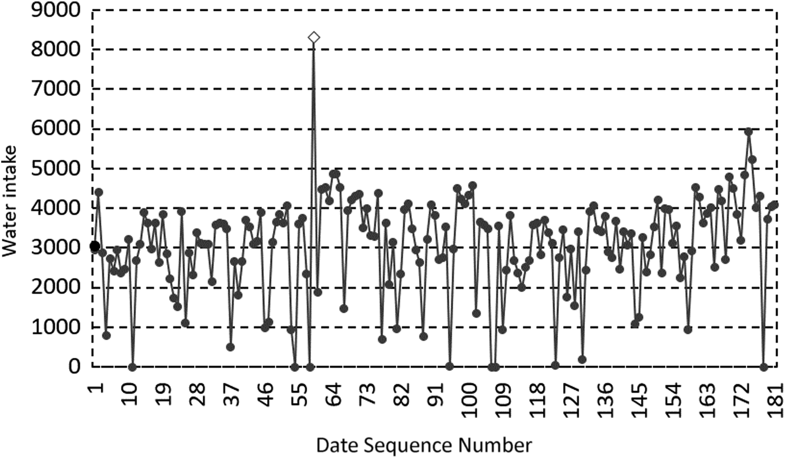
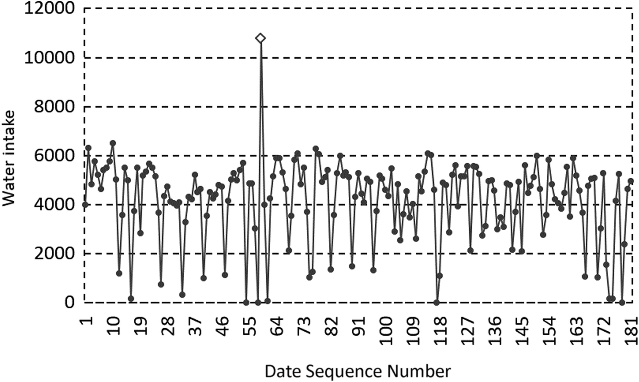
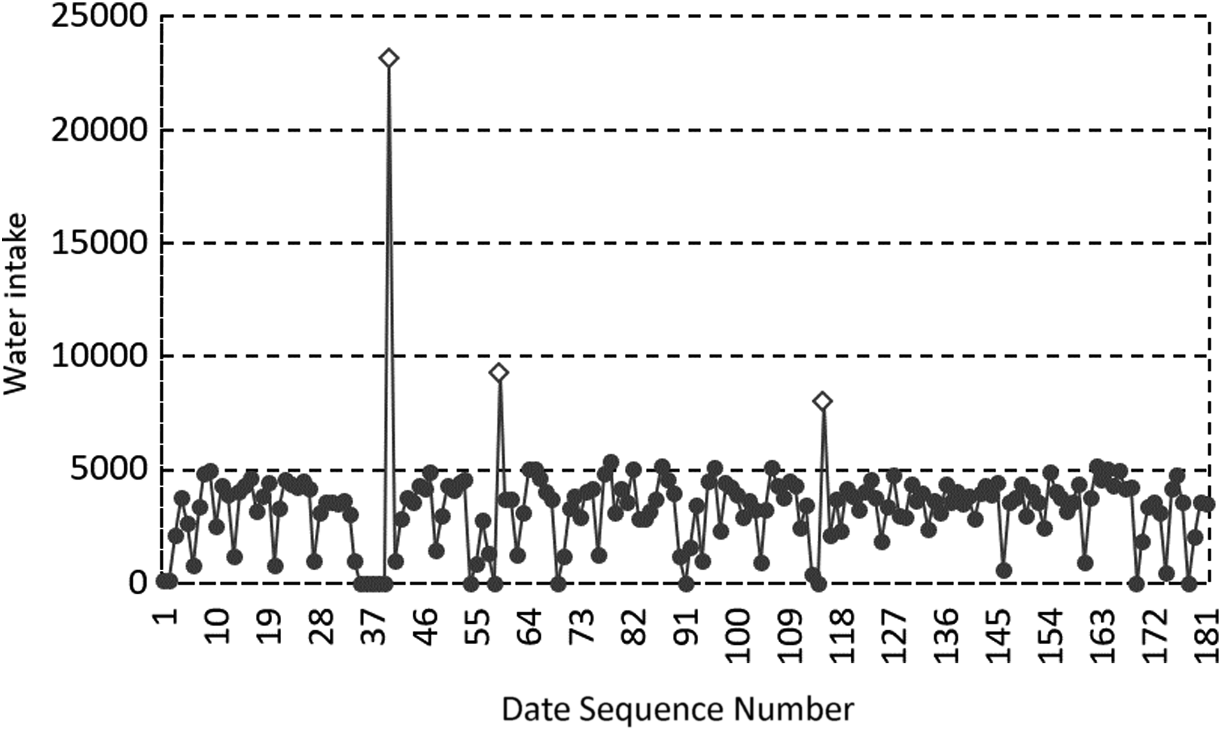
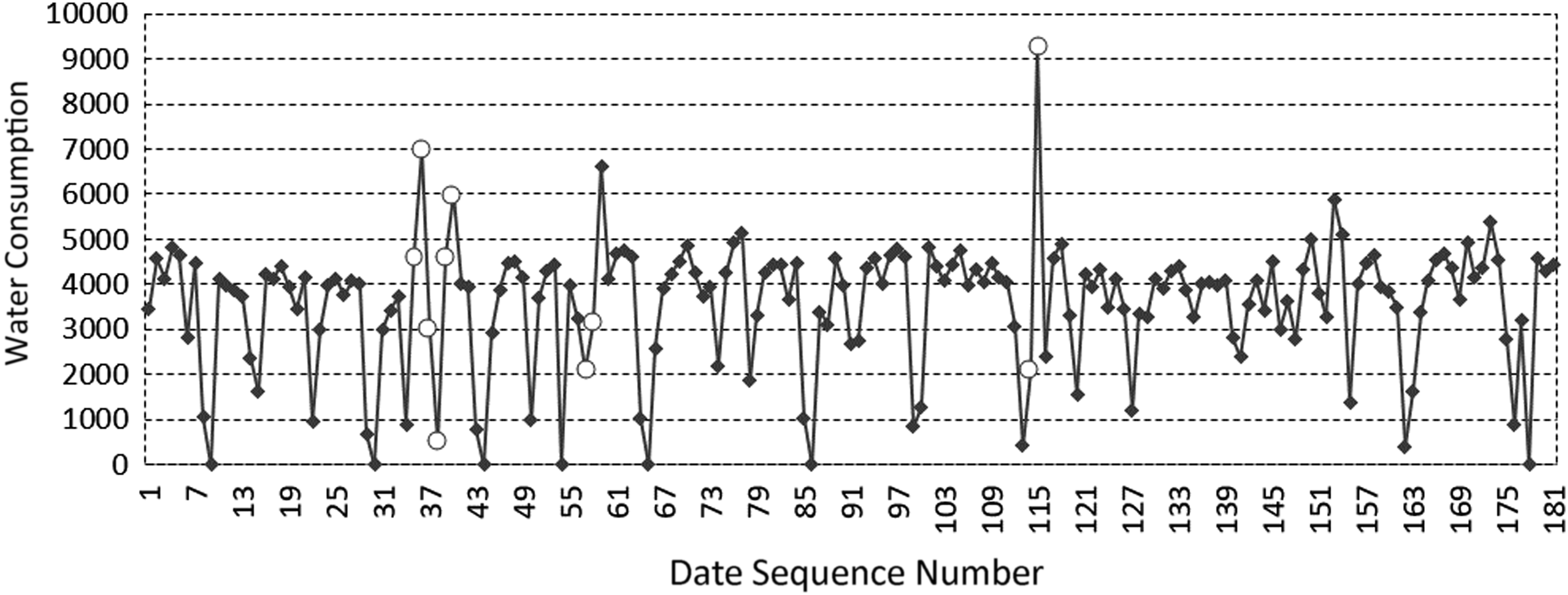
The ADRD algorithm is used to monitor and discriminate the water intake data of 2, 3, 4, and 6 stations of a water plant in Guangdong in the first half of 2017. The discriminant results of abnormal large values are shown in Figures 14–17.

OPEN IN VIEWER

FIG. 14.

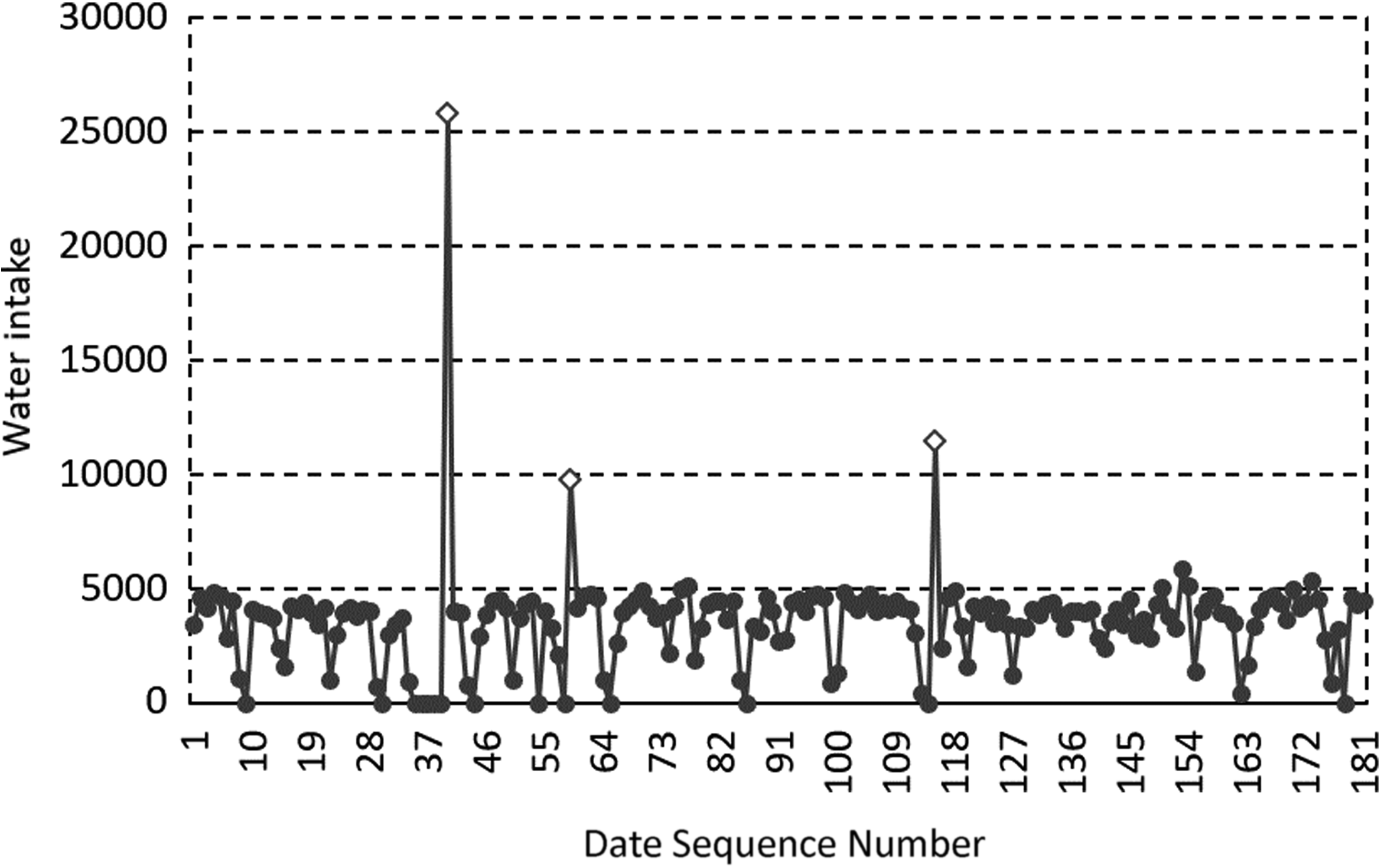
Abnormal large values discrimination result for MP 2 in the first half of 2017. Diamonds represent abnormal large values, and the circles represent the values of monitoring data.

OPEN IN VIEWER

FIG. 15.

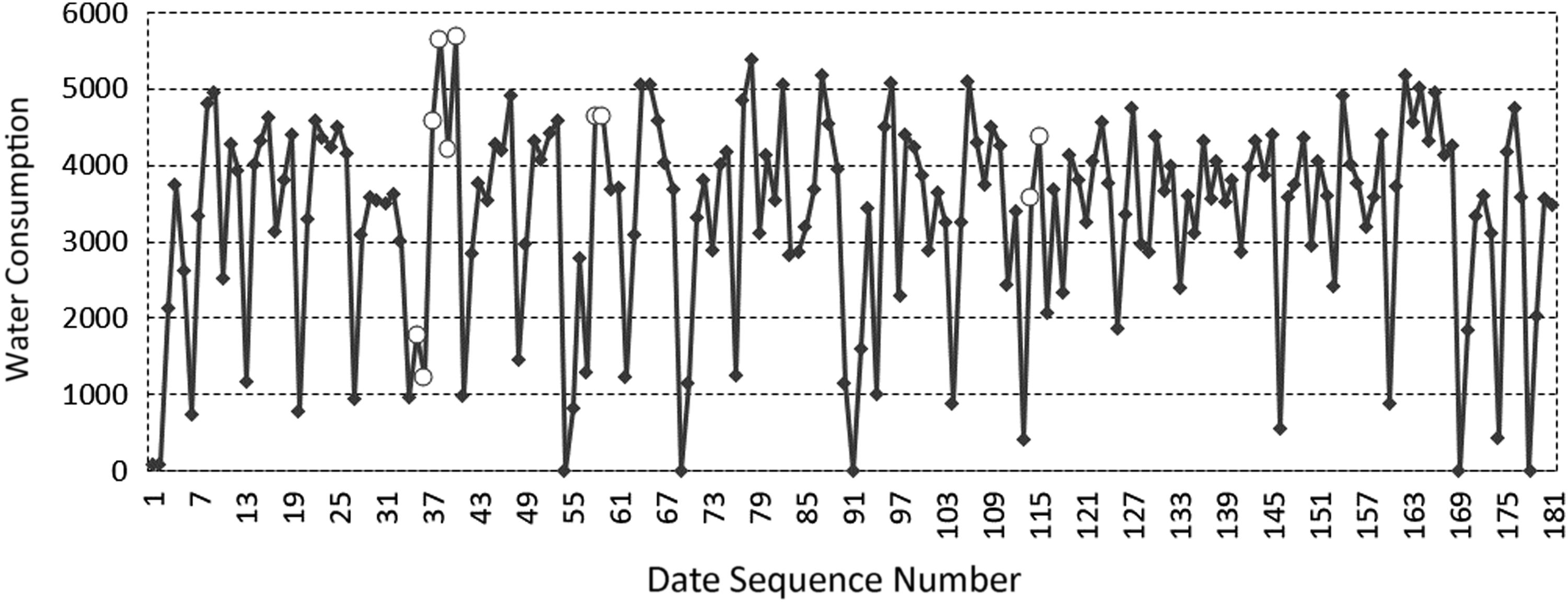
Abnormal large values discrimination result for MP 3 in the first half of 2017. Diamonds represent abnormal large values, and the circles represent the values of monitoring data.

OPEN IN VIEWER

FIG. 16.

Abnormal large values discrimination result for MP 4 in the first half of 2017. Diamonds represent abnormal large values, and the circles represent the values of monitoring data.

OPEN IN VIEWER

FIG. 17.

Abnormal large values discrimination result for MP 6 in the first half of 2017. Diamonds represent abnormal large values, and the circles represent the values of monitoring data.

From the experimental results, it can be seen that the abnormal large value region of the data set is significantly larger than the normal data set, and its characteristics are consistent with the theoretical analysis.

The abnormal regions in Figures 14 and 15, and the second and third abnormal regions in Figures 16 and 17 all contain two abnormal data, so the value is about twice as large as the central value of the normal value distribution region. The first abnormal regions in Figures 17 and 18 contain six abnormal data, which are significantly higher than the central value of the normal value distribution region. It can be seen that with the expanding of the abnormal data region, the abnormal large value increases proportionally, which is consistent with the analysis to the characteristics of the abnormal large value analyzed previously in the article.

OPEN IN VIEWER

FIG. 18.

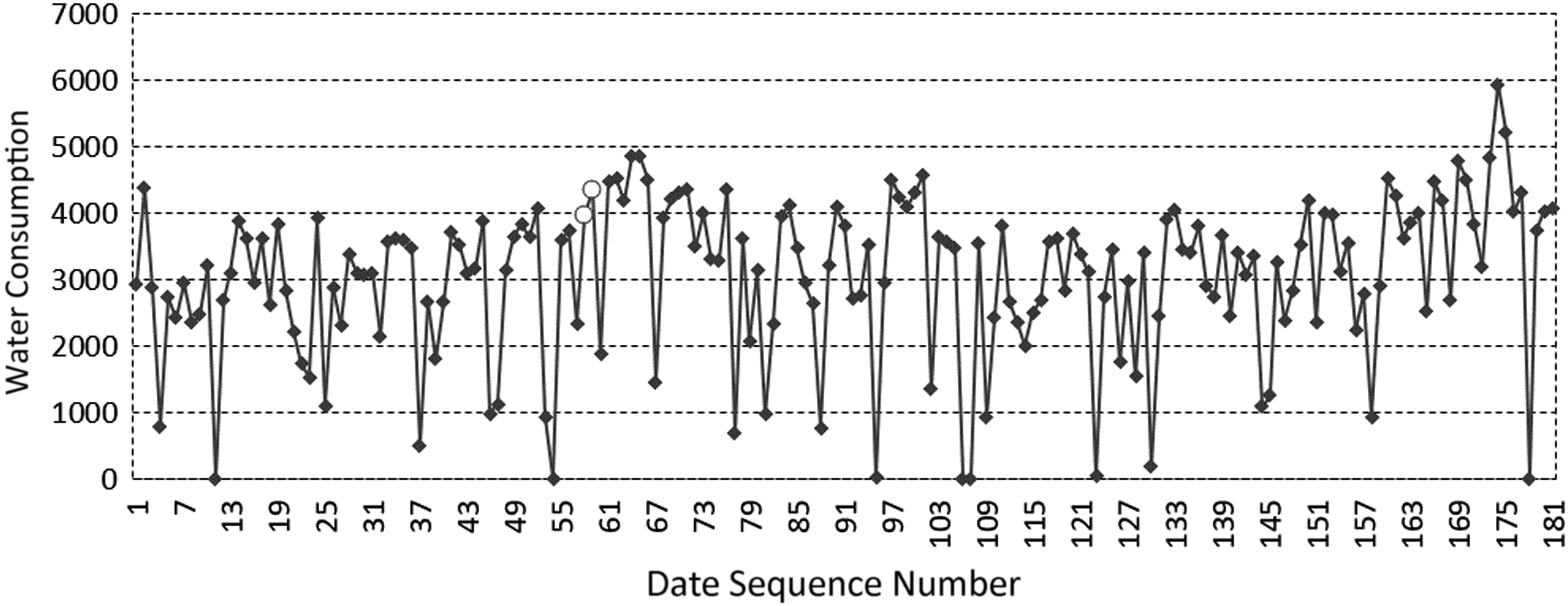
Repair results in the first half of 2017 for MP 2. Diamonds represent the values of monitoring data, and the triangles represent the repaired values.

The mentioned experiments show that the ADRD algorithm can correctly identify the abnormal data and locate the regions where abnormal data existed.

The mentioned parameters and statistical characteristics of the abnormal data were analyzed and calculated, and the results are given in Table 2.

OPEN IN VIEWER

Table 2.

Relation between the abnormal values and the expectations

MP No.	MP marking	Size of region	Monitoring value	Mean	Expectation ratio
2	2017.2.28	2	8297	3050.1	2.72
3	2017.2.28	2	10,780	4191.3	2.57
4	2017.2.9	6	23,108	3353.5	6.89
	2017.2.28	2	9255	3353.5	2.76
	2017.4.25	2	7977	3353.5	2.38
6	2017.2.9	6	25,730	3564.8	7.21
	2017.2.28	2	9747	3564.8	2.73
	2017.4.25	2	11,381	3564.8	3.19

MP, monitoring point.

It can be seen from Table 2 that when there are two elements in the abnormal region, the value range of the expectation ratio of measurement points is [2.57, 3.19], and the mean value is 2.73. When there are six elements in the abnormal region, the expectation ratio of measurement points is 6.89 and 7.21, respectively, and the mean value is 7.05. The results are in agreement with Equation (4), indicating the correctness of the proposed discrimination criterion. The characteristics of abnormal data can be highlighted by the proposed method.

CMHCR experiment and analysis

The data in the first half of 2017 were repaired by the CMHCR method. First, the correlation coefficient between the first half of 2017 and the first half of 2016 is calculated, as given in Table 3. In data processing, since February 2016 has 29 days, February 2017 has 28 days, so the data of February 29, 2016, have been removed to ensure the correspondence of the data.

OPEN IN VIEWER

Table 3.

Correlation coefficient of the data in the first half of 2016 and 2017

	16-1	16-2	16-3	16-4	16-5	16-6
17-1	−0.0707	−0.0829	0.0117	0.0385	0.1922	0.0811
17-2	0.2317	0.2182	−0.1353	−0.1452	−0.0221	−0.0785
17-3	0.2149	0.1725	−0.1723	−0.1149	−0.1235	−0.0363
17-4	−0.1095	0.0655	0.1170	0.0669	−0.0883	0.0265
17-5	−0.0933	−0.0216	−0.0877	−0.0255	0.0613	0.0145
17-6	−0.2086	−0.0048	0.0464	0.0029	0.0481	0.1361

According Table 3, the greatest correlation relation between 2017 data and 2016 data is MP 1 and MP 5, MP 2 and MP 1, MP 3 and MP 1, MP 4 and MP 3, MP 5 and MP 5, and MP 6 and MP 6. The maximum correlation coefficient was 0.2317 and the minimum correlation coefficient was 0.0613. The correlation characteristics were not obvious, but to other measuring points, the correlation was maximum. Comparing the data of Tables 3 and 1, the maximum correlation coefficient in Table 1 is 0.6022 and the minimum correlation coefficient is 0.3031, which are obviously higher than the results in Table 3.

This shows that although there is some correlation between the data of different measuring points, they are different physical measuring points after all. Theoretically, with the increase of measuring data capacity, the correlation between the two groups of data decreases. As the data capacity decreases, the correlation increases, so the correlation coefficient of local data is higher than the overall correlation coefficient.

For the corresponding relationship between the two data on the same day, CMHCR can be used to estimate missing data. From the previous analysis, we can see that in the first half of 2017, there are missing data in MP 2, 3, 4, and 6. The above algorithm was used to repair the missing data. The results are shown in Figures 18–21.

OPEN IN VIEWER

FIG. 19.

Repair results in the first half of 2017 for MP 3. Diamonds represent the values of monitoring data, and the triangles represent the repaired values.

OPEN IN VIEWER

FIG. 20.

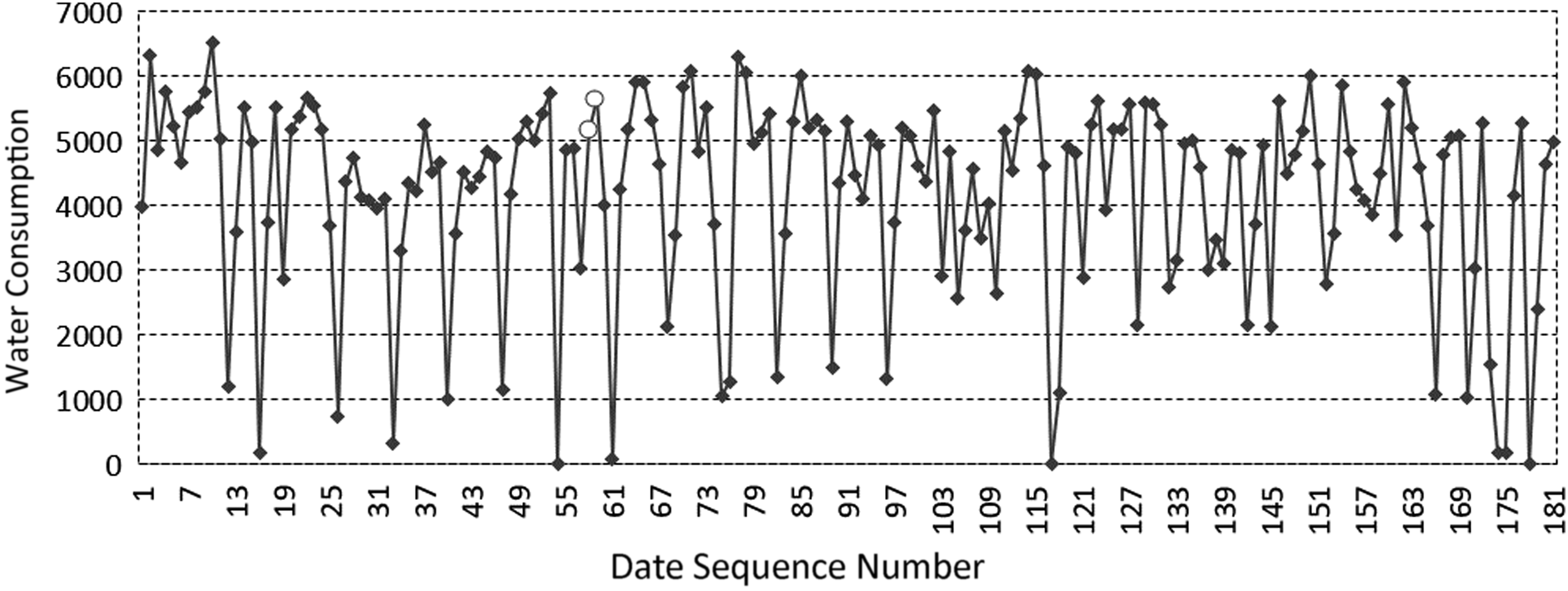
Repair results in the first half of 2017 for MP 4. Diamonds represent the values of monitoring data, and the triangles represent the repaired values.

OPEN IN VIEWER

FIG. 21.

Repair results in the first half of 2017 for MP 6. Diamonds represent the values of monitoring data, and the triangles represent the repaired values.

From the repair of MP 2 and MP 3, it can be seen that the results of the CMHCR method can effectively retain the normal maximum data, and there is no significant difference in the distribution of the data region after repair. For the repair data of MP 4, the first region and the third region have similar results as those of MP 2 and MP 3. In the data restoration of the second region, the repair formula is invalid because of the 0 value of the corresponding historical data. Therefore, equal weight is applied to deal with this situation, that is \documentclass{aastex}\usepackage{amsbsy}\usepackage{amsfonts}\usepackage{amssymb}\usepackage{bm}\usepackage{mathrsfs}\usepackage{pifont}\usepackage{stmaryrd}\usepackage{textcomp}\usepackage{portland, xspace}\usepackage{amsmath, amsxtra}\usepackage{upgreek}\pagestyle{empty}\DeclareMathSizes{10}{9}{7}{6}\begin{document} \begin{align*} { s \prime \prime _ { newk } } = \frac { 1 } { m } { s \prime _ { newm } } , k = 1 , 2 , \cdots , m. \tag { 9 } \end{align*} \end{document}

The results of repair data in the first and second regions of MP 6 are similar to the preceding results, but in the third region, the abnormal large values are still large after repair, but their changes are the same as the corresponding historical data regions, and they are consistent with the data changes before the abnormal large data, that is, the value of the third data before the abnormal large data is 3077, and the value of the second data is 410. The repair values are 2090.9 and 9290.1, respectively. In this case, the rationality analysis of abnormal large value repair needs further study.

Conclusion

This article analyzed the distribution characteristics of abnormal data region in actual water intake monitoring. According to the characteristics of 0 data plus abnormal large data and the numerical law of expectation of MPs, an ADRD algorithm is proposed. The algorithm can identify the normal 0 value region and the abnormal 0 value region, and determine the abnormal data region. For the abnormal data region, the correlation of the historical data in different MPs was analyzed. According to the conclusion of analysis, the current measurement data may not have the greatest correlation with the historical data of the corresponding node, but have the greatest correlation with the data in other MPs. Based on this, a CMHCR method was proposed.

The experimental results show the correlation of the data in the current MP and the data in different MPs are not linear, so the relative maximum correlation is used to repair. The proposed method is experimented with the monitoring data of a water plant in Guangdong Province in 2016 and 2017. According to the experimental results, the ADRD algorithm can effectively identify the abnormal data and locate the regions correctly. The CMHCR method can repair the abnormal data on the basis of maintaining the distribution characteristics of original data.