Fuzzy Inspired Deep Belief Network for the Traffic Flow Prediction in Intelligent Transportation System Using Flow Strength Indicators

Abstract

Intelligent transportation system (ITS) is an advance leading edge technology that aims to deliver innovative services to different modes of transport and traffic management. Traffic flow prediction (TFP) is one of the key macroscopic parameters of traffic that supports traffic management in ITS. Growth of the real-time data in transportation from various modern equipments, technology, and other resources has led to generate big data, posing a huge concern to deal with. Recently, deep learning (DL) techniques have demonstrated the capability to extract comprehensive features efficiently, using multiple hidden layers, from such huge raw, unstructured, and nonlinear data. Nonlinearity in traffic data is the major cause of inaccuracy in TFP. In this article, we propose a flow strength indicator-based Chronological Dolphin Echolocation-Fuzzy, a bioinspired optimization method with fuzzy logic for incremental learning of deep belief network. Technical indicators provide flow strength features as an input to the model. Hidden layers of DL architecture consequently learn more features and propagate it as an input to next layer for supervised learning. The degree of membership to the features is identified by the membership functions, followed by weight optimization using Dolphin Echolocation algorithm to fit the model for the nonlinear data. Experiments performed on two different data sets, namely Traffic-major roads and performance measurement system-San Francisco (PEMS-SF), show good results for the proposed deep architecture. The analysis of the proposed method using log mean square error and log root mean square deviation acquires a minimum value of 2.4141 and 0.61 for the Traffic-major roads database taken for the time step duration of 1 year and a minimum value of 1.6691 and 0.5208 for PEMS-SF data set for the time step interval of 5 minutes, respectively. These positive results demonstrate key importance of our traffic flow model for the transportation system.

Introduction

An effective traffic management system for road transportation depends on successful development and deployment of accurate traffic flow prediction (TFP) techniques in intelligent transportation system (ITS). Rapid developments in society have contributed to the massive existence of traffic in urban areas affecting transportation that lead to vehicle congestions or accidents¹ and generation of huge traffic data. Traffic data in transportation is increasing exponentially based on autonomous sources, heterogeneous characteristics, and evolving complex associations.^2,3 ITS uses various sensing devices including loops, cameras, mobile probes, or road-embedded to collect the values of these traffic data for the parameters, such as flow, density, and speed. Unlike other networks, road transportation networks are complex with abundant nonlinear data.⁴ Thus, the primary intention of ITS is to resolve the issues related to the road transportation by means of system engineering ideas, synergistic technologies to enhance and develop the transportation intelligently.^1,5 Macroscopic parameters of traffic flow information such as flow, speed, and density govern road transportation in ITS, which is essential for individual travelers, business sectors, and government agencies.⁶ Therefore, it is clear that an accurate and timely traffic flow information in traffic management is essential for the successful exploitation of ITS.⁷ TFP is an important task of ITS applications¹ based on the historical, current, and real-time data. TFP helps users to do an effective planning and avoid hectic impacts of traffic on the road links by providing alternate travel options to degrade traffic congestion, minimize carbon emissions, and enhance the efficiency of the traffic operation.⁸ Apart from dealing with the complex and dynamic traffic data,¹ prediction of traffic in an online and real-time environment provides solution to control and manage various traffic conditions.^9,10 Numerous mathematical models and classical Machine Learning algorithms were developed to deal with irregularity of traffic data. These models fail to capture the uncertainty and nonlinearity of time series data due to the traditional feature extraction method,¹¹ where the features are handcrafted for every new set of training data, which increases the cost and time consumed by the model. Another problem is to obtain prior knowledge of specific domains for feature extraction and selection process.

Effective traffic control and operations are affected due to the inherent nonlinearity, uncertainty, and complexity, as these factors degrade the accuracy of prediction.¹² An accurate prediction of traffic flow data on a particular road link supports ITS. Traffic information can be analyzed based two entities: first, based on the time series data known as temporal information, and, second, based on the junctions, links, and regions, known as spatial information. Temporal information provides support to find long-term and short-term TFP. Separate learning for different spatial segments makes the computational process complex and inefficient. ITS needs more accurate method to address both spatiotemporal traffic information.

All these issues led us to develop a novel method for predicting the traffic flow with better accuracy. The main objective of this research was to deal with the huge set of nonlinear traffic data for long-term and short-term TFP considering the spatiotemporal parameters. The proposed TFP method consists of two major steps. In the first step, leading and lagging indicators find the flow strength features of input data. Consequently, in the second step, granular features are extracted using the hidden layers fuzzified and integrated with Dolphin Echolocation (DE) optimization method for the prediction of traffic flow using deep belief network (DBN).

Traffic flow strength indicators

The role of these indicators is to predict traffic flow strength features effectively for the initial input data, and consequently, features are extracted by the deep architecture to understand the correlation between irregular nonlinear data. The indicators employed for evaluating and extracting the strength of the traffic flow include Momentum (MOM), Relative Strength Index (RSI), Commodity Channel Index (CCI), Average Directional Movement Index (ADX), and Triple Exponential Moving Average (TEMA). These indices are computed to represent the features of the input data.

Incremental Chronological Dolphin Echolocation-Fuzzy DBN

The main aim of this research was to focus on TFP using DBN, which is trained by proposing an optimization algorithm, named flow strength indicator-based Chronological Dolphin Echolocation-Fuzzy (CDE-Fuzzy) algorithm. The proposed algorithm inherits the features of input data and propagates in deep net to extract newer features. These features are fuzzified with fuzzy membership functions to obtain chronological data that are integrated in the weight update process of the DE algorithm that converges to obtain global optimal solution in DBN. The experimental results demonstrate that the proposed method for TFP outperforms the existing methods.

The rest of this article is organized as follows: The proposed strategy is explained in the Methodology section, whereas the Results and Discussion section deliberates the experiments and results of the proposed method, providing a comparative analysis. Finally, the Conclusion section concludes the article.

Literature review

This section provides reviews of the literature on various TFP techniques applied on the traffic data set obtained from various sources for addressing issues related to forecast accuracy, nonlinear data, long-term and short-term TFP, and spatiotemporal information.

Lv et al.⁸ developed a method, named deep learning (DL) approach with stacked Autoencoder-based TFP that was capable of yielding better prediction performance using logistic regression predictor, which may be extended with powerful predictor for further improvement in the performance. It has considered the spatiotemporal features but not applied and tested on huge data from different public open traffic data sets. Wibisono et al.¹³ established a method of predicting the traffic using “Fast Incremental Model Trees–Drift Detection (FIMT-DD)” that provides spatial traffic information and imposes a minimum error experience over the trained model but requires sufficiently huge traffic data to predict error performance for the traffic condition accurately. Hu et al.¹⁴ developed a method that solves the nonlinearity in data pattern using Particle Swarm Optimization in Support Vector Regression with better prediction results in the presence of noises. The model is applicable for the short-term traffic flow prediction. It specifies temporal information but does not address the extraction of spatial features to predict the traffic flow. Li et al.¹² developed a method named “Multivariate Data Fusion” with Bayesian theory and radial basis function to deal with chaotic characteristics of traffic flow. The study addresses about short-term TFP accurately but fails to deal with congested traffic conditions (nonlinearity) using multiple measures. Xia et al.⁹ developed a “Map Reduce-based Nearest Neighbor” approach that improved the efficiency and scalability of TFP, saved memory consumption, and reduced the computational costs. However, the method does not address the nonlinearity for large training samples. Zhao and Su¹ modeled a Gaussian Process Dynamical Model (GPDM) that performs better and offers significant improvements in traffic prediction performance. The demerit of the method is that it cannot use the mixtures of GPDMs to model time series. Oh et al.¹⁵ developed the Multifactor Pattern Recognition Model, which offers a highly reliable prediction. However, the method cannot handle heavy traffic congestion, which leads to the problem of nonlinear data pattern. Vasantha Kumar and Vanajakshi¹⁶ developed a Seasonal Autoregressive Integrated Moving Average (SARIMA), a data-driven model, that employs limited input data for TFP. Limited spatiotemporal information is learnt for traffic prediction. In the study by Yanchong et al.,¹⁷ an approach was developed for predicting short-term traffic flow using the wavelet analysis and neural network (NN). Here, the traffic flow data was partitioned into low- and high-frequency signals through wavelet decomposition. Then, back propagation NN processes the decomposed signal for the prediction.

A hybrid automaton modeling was developed by Banjanović-Mehmedović et al.¹⁸ under varying platooning conditions with nonlinear autoregressive network (NARX) NN-based prediction in ITS. Hybrid automaton considers the nonlinear dynamics of every vehicle and provides a better forecasting using the NARX prediction. Huang et al.¹¹ introduced a deep architecture for TFP, which employs a stack of Restricted Boltzmann Machines (RBMs) at the bottom with a regression layer at the top. The DBN-based TFP is effective for unsupervised feature learning. However, the problem of how to employ temporal information in TFP is a challenge in this approach. In addition, this approach shows constraints for real-time applications.

Koesdwiady et al.¹⁹ developed a complete prediction architecture, which includes DBNs and data fusion for developing a perfect TFP in San Francisco, Bay Area. This method utilized the weather data and a traffic flow history. This method guaranteed better prediction and management of traffic strategies. Yang et al.²⁰ introduced a stacked Autoencoder Levenberg-Marquardt model for traffic flow forecasting. This model was designed by the Taguchi scheme for developing an optimized structure and discovering the traffic flow features via layer-by-layer feature granulation with a greedy layer-wise unsupervised learning algorithm. This model had higher performance in traffic flow forecasting. Jia et al.²¹ analyzed the performance of the long short-term memory (LSTM) and DBN for performing the short-term traffic speed prediction with the rainfall impact. The DL discovered the complex features of the traffic flow pattern under a variety of rainfall conditions. Tian and Pan²² proposed a model named Long Short-Term Memory Recurrent Neural Network (LSTM RNN), which took the benefits of the three multiplicative units in the memory block for finding the optimal time lags energetically. This prediction model avoids gradient vanishing–exploding problem for nonlinear data, obtains higher accuracy, and generalizes well. Luo et al.²³ introduced a spatiotemporal traffic flow model combined with k-nearest neighbor (KNN) and LSTM network, which is named KNN-LSTM model. KNN was used to select mostly related neighboring stations with the test station and to capture spatial features of traffic flow. LSTM was used to mine temporal variability of traffic flow, and a two-layer LSTM network was applied to predict traffic flow respectively in selected stations. The final prediction results were attained by result-level fusion with rank-exponent weighting approach. However, the method produces good prediction accuracy, but further improvement is required due to the nonlinearity caused by weather, incident, and other factors.

Summary and motivation

The issues observed from the existing work need improvement in terms of forecasting accuracy. A development of unified model is required to handle big data, computational cost involved, effects of nonlinear traffic data on traffic condition, and exploration of spatiotemporal traffic dependency, as well as, to address the challenges in long-term TFP.

Multifaceted algorithms are developed in TFP using parametric and nonparamedic approach,²⁴ but it is difficult to state the dominance of one algorithm over the other. Since each model uses different techniques, considering limited contextual factors, environment affects, and available data set.²⁵ Of the context researcher started exploiting hybrid methods,²⁶ the existing methods were compared to predict traffic flow accuracy integrating newer concept to identify the features embedded^8,27 in the collected spatiotemporal traffic data.

With the popularity and capability of DL methods, which address massive data, DL methods stand as a good option for handling the learning process associated with the complex nonlinear data carrying high-dimensional features²⁸ and optimized structure.²⁹ DL deals with problems such as classification, dimensionality reduction, natural language processing, motion modeling, and object detection.^30,31 DL algorithms exhibit multiple-hidden layer for unsheathing the inherent features of data from the lowest to the highest level.²⁵ Eventually, it is clear that using DL algorithms, we can predict the traffic flow without any prior knowledge of the traffic despite its complexity⁸ and exhibit better performance.

These capabilities led us to work more on a DL model to develop a novel method for predicting the traffic flow with better accuracy. In this article, we explore a DL approach with technical indicators, fuzzy membership functions, and bioinspired optimization algorithm over DBN for TFP.

Methodology

The major concern for the TFP model is to deal with the huge raw data obtained from various resources. Some of the standard data set provides well-structured data. The raw data obtained through the data set need to be preprocessed based on the problem domain, algorithmic approach, and computational need. Generally, the characteristics of traffic data are nonlinear due to the contextual factors such as traffic incidents, constructions, public events, and weekdays in the time series data. Prediction based on historical, current, and real-time data contains the traffic data of the road links at various places. Even though there are many techniques employed in predicting the traffic flow, the prediction accuracy is yet another factor to be concentrated. The proposed method predicts the traffic flow through the extraction of the traffic flow strength features from the time series data. The traffic flow features are given as input to the CDE-Fuzzy-based DBN model.

The traffic flow predictor uses DBN tuned by CDE-Fuzzy algorithm, which inherits the advantages of fuzzy membership and chronological property integrated in the DE algorithm. Figure 1 shows the block diagram of the TFP method using the proposed CDE-Fuzzy DBN.

FIG. 1.

Block diagram of the CDE-Fuzzy DBN technique for TFP. CDE-Fuzzy, Chronological Dolphin Echolocation-Fuzzy; DBN, deep belief network; TFP, traffic flow prediction.

Extraction of traffic flow strength features

This section deliberates the traffic flow technical indicators and the procedure to compute the flow strength features as an initial input to the proposed model for predicting the flow. Generally, technical indicators³² are employed for computing the stock exchange flow and proven effective predictors of features, such as change in price, stock trend, buy and sell, signal and noise elimination, and data smoothing in stock prices.³³ Thereby, assure the prediction of the close pricing of the stocks prevailing in different markets. We have used these stock-based technical indicators for extracting flow strength features of the traffic data. The extraction of initial traffic flow strength features is obtained by modeling the traffic indicators that effectively help in tuning the input data for the proposed model. Subsequently, features are extracted in the deep net by the hidden layers for accurate prediction of flow. Generally, traffic flow indicators come under two major classes: leading, an input-oriented indicator, and lagging, an output-oriented indicator. Using the historical traffic flow data, the leading indicators ensure the prediction of the traffic flow in the future, whereas the lagging indicators help to identify the change in traffic flow. We have used five indicators, namely MOM, RSI, CCI, ADX, and TEMA.³² The indicators, such as MOM, RSI, and CCI, are leading indicators that help to extract features and provide information for the future traffic flow. ADX is a lagging indicator that measures the up and down of traffic flow based on past data. TEMA reduces the lags between the indicators and helps in smoothing the flow fluctuations, thereby predicting the traffic flow without the lag associated with the traditional moving average. Modeling of flow strength features using the indicators is explained below.

Momentum

MOM refers to the rate of rise or falls in the traffic flow rate and represented by Equation (1). $M = T^{t} - T^{t - n},$ (1)

where T^t is the traffic flow rate at the time t, $T^{t - n}$ is the traffic flow rate at the time $(t - n)$ , and n specifies the time step duration (intervals) in years or minutes.

Traffic flow rate is defined as the number of vehicles passes through a given point per hour on the roadway.³⁴

Relative Strength Index

RSI is the measure of the change in the traffic flow rate over time t by comparing the magnitude of the recent increase and decrease of the traffic flow rate. The RSI formula is given as $R S I = \frac{A (T^{u})}{A (T^{u}) + A (T^{d})} \times 100,$ (2)

where $A (T^{u})$ refers to the average of the high value of the traffic flow rate and $A (T^{d})$ refers to the average of the low value of the traffic flow rate. These are calculated as $A (T^{u}) = 1 \times [T^{t} - T^{t - 1}]; (T^{t} - T^{t - 1}) > 0,$ (3)

A (T^{d}) = 1 \times [T^{t - 1} - T^{t}]; (T^{t} - T^{t - 1}) < 0 .

(4)

The traffic flow rate-up is the difference between the traffic flow rate at time t and time $(t - 1)$ , whereas the traffic flow rate-down is the difference between the traffic flow rates at time $(t - 1)$ and time t.

Commodity Channel Index

CCI is the measure of the variation in the typical traffic flow rate relative to the predefined moving average to the 1.5% of the normal deviation from that average. The CCI is defined as $C C I = \frac{P^{t} - A (P^{t}, n)}{0.15 \times N^{t}},$ (5)

where $P^{t} = \frac{h^{t} + b^{t} + c^{t}}{3}$ , wherein h^t denotes the higher traffic flow rate at the time t, b^t specifies the low traffic flow rate at the time t, and c^t indicates the close value of the traffic flow rate at the time t. The CCI enables the predictors to measure the rate at which traffic flow increase and decrease, or in other words, the change in the traffic flow rate is noticed by this measure. The predefined moving average is computed as $A (P^{t}, n) = \frac{(P^{t} + P^{t - 1} + \dots + P^{t - (n + 1)})}{n + 2} .$ (6)

The normal deviation is defined as $N^{t} = A |P^{t} - A (P^{t}, n)| .$ (7)

Equation (7) is computed as the average of the difference between the absolute value of the typical traffic flow rate and the predefined moving average that is the average of the typical traffic flow rate.

Average Directional Movement Index

ADX is the indicator that defines the strength or weakness of the flow trend irrespective of increase or decrease in the traffic flow rate based on the plus and minus directive index. When the traffic flow rate increases, the difference between the present high and previous high values of the traffic flow rate is considered as a plus directive index. Similarly, when the traffic flow rate decreases, the minus directive index is determined as the difference between the present low and previous low values of the traffic flow rate. The plus directional movement is determined as $A D X = \frac{s u m [\frac{+ D I - (- D I)}{+ D I + (- D I)}]}{n},$ (8)

where $+ D I$ refers to the plus directional index and $- D I$ refers to the minus directional index. The directional index is the ratio of the directional movement to the true range (TR). The plus directional index is given as $+ D I = \frac{+ D M}{T R} \times 100,$ (9)

where $+ D M$ is the plus directional movement of the traffic flow rate at the time t. +DM = Current High − Previous High. The minus directional index is given as $- D I = \frac{- D M}{T R} \times 100,$ (10)

where $- D M$ is the minus directional movement of the traffic flow rate at the time t. −DM = Previous Low − Current Low. The TR is formulated as $T R = \frac{D I}{n},$ (11)

where n is the total time interval. The directive index is based on the traffic flow rate-up and the traffic flow rate-down. If the traffic flow rate-up exceeds the traffic flow rate-down and exceeds zero, the plus directive index is notified as the traffic flow rate-up or else it becomes zero. When the traffic flow rate-down is greater than the traffic flow rate-up and exceeds zero, the minus directional index is notified as the traffic flow rate-down or else it becomes zero. TR is the ratio of the directive index to the total number of traffic instances in the time series database.

Triple Exponential Moving Average

TEMA is a measure that smoothens the variations in the traffic flow rate, filters out the volatility, and makes the ability to determine the trends with minimum lag. It is the ratio of the traffic flow rate at the time t to the traffic flow rate at the time $(t - 1)$ . TEMA is formulated as $T E M A = \frac{T R^{t}}{T R^{t - 1}},$ (12)

where $T R^{t} = E M A [E M A (E M A (T^{t}))]$ for n days and $E M A$ is the exponential moving average.

The traffic strength indicators are organized as the feature vector of dimension $[1 \times 5]$ , represented as, $F = \{F_{1}, F_{2}, F_{3}, F_{4}, F_{5}\},$ (13)

where F₁ indicates the MOM feature, F₂ specifies the RSI feature, F₃ indicates the CCI feature, F₄ refers to the ADI feature, and F₅ specifies the TEMA feature. The extracted flow features obtained from the traffic data are given as input to the deep net model.

CDE-Fuzzy algorithm for training the DBN

The traffic flow input data from the data set are incremental as the traffic data keeps on updating frequently. DBN is capable of dealing with unsupervised prelearning for incremental data. Hence, the prediction model based on the DBN serves as a better platform to train and test in predicting the traffic flow based on the historical traffic flow data. The traffic flow data is dynamic in nature and varies with time, insisting the need for better classification for the incremental data. The proposed DBN is fine-tuned with the supervised learning, which uses target labels to perform regression analysis and paves an effective platform to predict the future traffic using the core features obtained by the indicators.

The developed CDE-Fuzzy algorithm, which is the integration of Chronological and fuzzy theory in the DE optimization algorithm, trains the DBN. The DE algorithm³⁵ inherits the sophisticated bio sonar system such that the dolphin's track discriminate, locate the prey, and thereby solve the prey-intercept objective. Sonar is an attractive mechanism in dolphin employed to avoid the obstacles and locate the prey in the search space. Dolphin generates the clicks and evaluates the energy of the captured click to locate the distance of the prey from the dolphin. Dolphin concentrates on the particular target by increasing the generation of clicks. Thus, the DE algorithm local investigation optimizes the parameters and supports global exploration for effective computation. The optimization algorithm offers a flexible solution and is suitable for solving the multiple constraint objective functions, but the convergence requires further improvements due to the existence of nonlinear data.³⁶ So, to improve the convergence rate, the proposed algorithm inherits the advantages of fuzzification through the degree of membership functions to the features obtained from the technical indicators under chronological order in DE optimization algorithm. The fuzzy concept³⁷ gains significance because of its flexibility to precisely categories each traffic feature. It does this by emphasizing on imprecise and incomplete traffic data and models the nonlinear functions with arbitrary functions. Fuzzy holds simple computations and covers a large range of traffic features in the updating process.

Derivation of the update rule using the proposed CDE-Fuzzy-based algorithm

The CDE-Fuzzy algorithm for computing the optimal weights of the DBN is developed by modifying the update rule of the DE algorithm using the fuzzy and chronological concept. The developed update rule ensures a better convergence rate and thereby enhances the flexibility and stability with high prediction accuracy. The standard equation of DE is given as $\begin{matrix} W_{k l} (z + 1) & = W_{k l} (z) + K_{k l} (z) + F [W_{k l} (z)] [L_{K L} - W_{k l} (z)] \\ + G [W_{k l} (z)] [g^{b e s t} - W_{k l} (z)] . \end{matrix}$ (14)

Rearranging the above equation, we get $\begin{matrix} W_{k l} (z + 1) & = W_{k l} (z) [1 - F [W_{k l} (z) - G [W_{k l} (z)]]] \\ + K_{k l} (z) + F [W_{k l} (z)] L_{k l} + G [W_{k l} (z)] g^{b e s t}, \end{matrix}$ (15)

where $W_{k l} (z + 1)$ is the position of the $l t h$ dolphin in the $k t h$ dimensional space at $(z + 1) t h$ iteration and $W_{k l} (z)$ is the position of $l t h$ dolphin in $k t h$ dimensional search space at $z t h$ iteration. The search space of the $l t h$ dolphin is notated as K_l. The local best and the global best solutions of the $l t h$ dolphin are denoted as $L_{k l}$ and $g^{b e s t}$ , respectively. The standard DE algorithm uses two random numbers in the interval $[0, 1]$ . However, in the CDE-Fuzzy algorithm, these random numbers are replaced using the fuzzy concept to represent the features, that is, the fuzzy triangular membership function, $F [W_{k l} (z)]$ , and the Gaussian membership function, $G [W_{k l} (z)]$ . The fuzzification is exhibited by selecting the triangular membership function for transforming the input feature vector into fuzzified value.³⁸

The fuzzy triangular memberships are given as $F [W_{k l}] = \{\begin{matrix} 0 & ; & i f W_{k l} \leq p \\ \frac{W_{k l} - p}{q - p} & ; & i f p \leq W_{k l} \leq q \\ \frac{r - W_{k l}}{r - q} & ; & i f q \leq W_{k l} \leq r \\ 0 & ; & i f W_{k l} \geq r \end{matrix},$ (16)

where p, q, and r are the lower, middle, and center boundary. The three vertices of the membership functions arep, q, and r of $F [W_{k l}]$ in a fuzzy set. The membership degree in the upper boundary is zero, and the membership degree in the middle fuzzy boundary is 1.

The Gaussian fuzzy $G [W_{k l} (z)]$ is given as $G [W_{k l} (z)] = \frac{1}{σ \sqrt{2 a}} e^{- \frac{1}{2} {(\frac{W_{k l} - μ}{σ})}^{2}},$ (17)

where μ is mean and σ is the standard deviation.

The membership functions utilize any structure for its applicability in the real-time applications.

The position of the $l t h$ dolphin in the previous iteration can be written as $\begin{matrix} W_{k l} (z) & = W_{k l} (z - 1) + K_{k l} (z - 1) + F [W_{k l} (z - 1)] \\ [L_{k l} - W_{k l} (z - 1)] + G [W_{k l} (z - 1)] \\ [g^{b e s t} - W_{k l} (z - 1)] \end{matrix}$ (18)

where $W_{k l} (z)$ is the position of dolphin in $z t h$ iteration. $W_{k l} (z - 1)$ and $K_{k l} (z - 1)$ are the position and search space of dolphin in $(z - 1) t h$ iteration.

Substituting Equation (18) in Equation (15), we get $\begin{matrix} W_{k l} (z + 1) & = [\begin{matrix} W_{k l} (z - 1) + K_{k l} (z - 1) + \\ F [W_{k l} (z - 1)] [L_{k l} - W_{k l} (z - 1)] + \\ G [W_{k l} (z - 1)] [g^{b e s t} - W_{k l} (z - 1)] \end{matrix}] \\ [1 - F [W_{k l} (z) - G [W_{k l} (z)]]] + K_{k l} (z) \\ + F [W_{k l} (z)] L_{k l} + G [W_{k l} (z)] g^{b e s t} \end{matrix} .$ (19)

Based on the chronological concept, the position of dolphin in $(z + 1) t h$ iteration is given as $W_{k l} (z + 1) = \frac{W_{k l} (z + 1) + W_{k l} (z + 1)}{2} .$ (20)

The chronological concept uses historical records so that the prediction using the proposed CDE-Fuzzy algorithm becomes effective and accurate. The chronological concept is merged in the DE algorithm through the substitution of Equations (19) and (15) in Equation (20) as $W_{k l} (z + 1) = \frac{1}{2} \{\begin{matrix} W_{k l} (z) [1 - F [W_{k l} (z) - G [W_{k l} (z)]]] + K_{k l} (z) + F [W_{k l} (z)] L_{k l} + G [W_{k l} (z)] g^{b e s t} + \\ [\begin{matrix} W_{k l} (z - 1) + K_{k l} (z - 1) + \\ F [W_{k l} (z - 1)] [L_{K L} - W_{k l} (z - 1)] + \\ G [W_{k l} (z - 1)] [g^{b e s t} - W_{k l} (z - 1)] \end{matrix}] [1 - F [W_{k l} (z) - G [W_{k l} (z)]]] + \\ K_{k l} (z) + F [W_{k l} (z)] L_{k l} + G [W_{k l} (z)] g^{b e s t} \end{matrix}\} .$ (21)

Algorithmic steps

The algorithmic steps of the CDE-Fuzzy weight optimization are depicted in Algorithm 1.

Algorithm 1.

Pseudocode of CDE-Fuzzy weight optimization

CDE-Fuzzy-based weight optimization
1	Input: Dolphin population
2	Output: Optimal position of dolphin (Optimal weights)
3	Begin
4	Initialization of the population
5	Determine the predefined probability
6	Evaluate the fitness of the solutions based on error
7	Update the search space dimension and position of dolphins
8	{
9	Update the position of dolphin based on the proposed update Equation (21).
10	}
11	Update the local and the global best solutions
12	Return $W_{k l} (z + 1)$ , best position of dolphins.
13	Terminate

Prediction of the traffic flow using the proposed CDE-Fuzzy DBN

This section deliberates the prediction of the traffic flow using the CDE-Fuzzy algorithm-based DBN.

The architecture of DBN

The importance of time series DBN³⁹ is to extract and recognize the patterns underlying in the data sequences. DBN is trained on the labeled data to minimize the error and thereby to predict the traffic using the outputs previously recorded to assure better prediction accuracy. The basic structure of DBN consists of multiple RBMs and a Multi-Layer Perceptron (MLP) layer. An individual layer of RBM and MLP resembles the architecture of NN. The layers are constructed with the interconnection of the neurons. In the incremental DBN, we have considered two RBM layers, and the input to the RBM1 is the feature vector corresponding to the traffic flow data. The inputs are multiplied with the weights of the parametric features to produce the output of the hidden layer, which forms the input to the RBM2. The inputs in RBM2 are processed with the hidden weights of RBM2 to obtained inputs to the MLP layer, which processes the weights and determines the final output. The weights of the DBN are updated using the CDE-Fuzzy Algorithm 1 until it converges to global optima. The architecture of the incremental DBN is depicted in Figure 2.

FIG. 2.

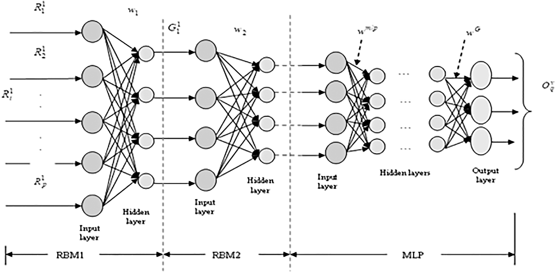
The architecture of incremental DBN model.

The mathematical model of the incremental DBN is framed as follows: There are two RBM layers, RBM1 and RBM2, and the input to the RBM1 is the feature vector (traffic flow strengths features) of the incoming traffic flow data. The input and the hidden neurons in the input layer of RBM1 are given as $R^{1} = {R_{1}^{1}, R_{2}^{1}, R_{3}^{1}, \dots, R_{i}^{1}, \dots, R_{p}^{1}}; 1 \leq i \leq p,$ (22)

G^{1} = {G_{1}^{1}, G_{2}^{1}, \dots, G_{j}^{1}, \dots, G_{y}^{1}}; 1 \leq j \leq y,

(23)

where $R_{i}^{1}$ is the $i t h$ input neuron present in RBM1, and the number of the input neurons in RBM1 is equal to the dimension of the feature vector. There are p number of neurons in the input layer of RBM1, and there are five flow strength indicators to perform the feature extraction. Let us represent the total number of the hidden neurons in the RBM1 as y and let the $j t h$ hidden neuron in RBM2 is denoted as $G_{j}^{1}$ . Let the biases in the visible and the hidden neurons of RBM1 are represented as $Q^{1} = {Q_{1}^{1}, Q_{2}^{1}, Q_{3}^{1}, \dots, Q_{i}^{1}, \dots, Q_{p}^{1}},$ (24)

U^{1} = {U_{1}^{1}, U_{2}^{1}, \dots, U_{j}^{1}, \dots, U_{y}^{1}} .

(25)

The biases in the hidden and the input layer of RBM1 equal to the total neurons in both the layers. The weights of the RBM1 are given as, $w^{1} = \{w_{i j}^{1}\}; 1 \leq i \leq p; 1 \leq j \leq y,$ (26)

where $w_{i j}^{1}$ indicates the weights of the RBM1 between the $i t h$ input neuron and $j t h$ hidden neuron of RBM1. The dimension of the weights is given as $(p \times y)$ . Thus, the output from RBM1 is $G_{j}^{1} = σ [U_{j}^{1} + \sum_{i} F_{i}^{1} w_{i j}^{1}],$ (27)

where $σ$ specifies the activation function in RBM1 and $F_{i}^{1}$ refers to the feature vector as in Equation (13). The output from RBM1 is given as $G^{1} = {G_{j}^{1}}; 1 \leq j \leq y .$ (28)

The output from RBM1 is provided as input to the RBM2, and the output of RBM2 is computed similarly based on the equations shown above. The output from RBM2 is represented as $G_{j}^{2}$ that is given as input to MLP layer. The input neurons in MLP are given as $W^{v} = {W_{1}^{v}, W_{2}^{v}, \dots, W_{j}^{v}, \dots, W_{y}^{v}} = {H_{j}^{2}}; 1 \leq j \leq y,$ (29)

where y is the total number of input neurons in the MLP layer. The hidden neurons of MLP are given as, $K^{v} = {K_{1}^{v}, K_{2}^{v}, \dots, K_{r}^{v}, \dots, K_{m}^{v}}; 1 \leq r \leq m,$ (30)

where m specifies the total number of hidden neurons in the MLP. The bias of the hidden neurons is given as $O^{v} = {O_{1}^{v}, O_{2}^{v}, \dots, O_{q}^{v}, \dots, O_{S}^{v}}; 1 \leq q \leq S,$ (31)

where S is the number of output neurons in the MLP layer. The weights between the input and the hidden layers are represented as $w^{m l p} = {w_{j r}^{m l p}}; 1 \leq j \leq y; 1 \leq r \leq m,$ (32)

where $w_{j r}^{m l p}$ is the weight vector between $j t h$ input neuron and $r t h$ hidden neuron. The output from the hidden layer in MLP is based on the bias and weights, and the output is given as $J = [\sum_{j = 1}^{y} w_{j r}^{m l p} \times L_{j}] w_{r}^{v} \forall L_{j} = {G_{j}}^{2},$ (33)

where $w_{r}^{v}$ is the bias of the hidden layer. The weight vector between the hidden and the output layer is indicated as $ω^{G}$ and is given by $w^{G} = {w_{r q}^{G}}; 1 \leq r \leq m; 1 \leq q \leq S .$ (34)

Thus, the output of MLP is computed as $O_{q} = \sum_{r = 1}^{m} w_{r q}^{G} \times J,$ (35)

where $w_{r q}^{G}$ denotes the weights between the hidden and output neurons in MLP and J is the output from the hidden layer.

(a) Training phase of RBM layers: The training of the RBM1 and RBM2 layers is performed based on the CDE-Fuzzy algorithm that derives the weights to obtain minimum error.

(b) Training of MLP layer: The steps involved in training the MLP layer are listed below:

Step 1: Randomly generate the weight vectors w^G and $w^{m l p}$ as shown in Equations (34) and (32), respectively.

Step 2: Read the input vector ${G_{j}}^{2}$ obtained from the output layer of RBM2.

Step 3: Calculate J and O_q based on Equations (33) and (35), respectively.

Step 4: Compute the error of the MLP layer using the estimated and target output as given below

{\in^{1}}_{a v g} = \frac{1}{ℜ} \sum_{x = 1}^{ℜ} {(O_{q} - g)}^{2},

(36)

where O_q is the attained output, g is the expected output, and $ℜ$ is the total number of training samples.

Step 5: Update the weight using the proposed CDE-Fuzzy-based algorithm: The weights of the MLP layer are updated based on the Equation (21), which is the update derived using the CDE-Fuzzy algorithm. The CDE-Fuzzy algorithm derives the optimal weights for predicting the traffic flow.

Step 6: Calculate the average error function ${\in^{1}}_{a v g}$ based on the weight vector, which is updated using the CDE-Fuzzy algorithm.

Step 7: Repeat steps 2 to 6, until the best weight vector is determined.

The CDE-Fuzzy-based DBN predicts the traffic flow optimally and supports the decision-making in an effective way.

Results and Discussion

This section depicts the results and discussion of the proposed model for predicting the traffic flow and the effectiveness of the CDE-Fuzzy DBN method using the comparative analysis.

Experimental setup

The experimentation is performed using the MATLAB tool, and the analysis is progressed using the Traffic-major roads⁴⁰ and performance measurement system-San Francisco (PEMS-SF)⁴¹ data sets. Table 1 shows the parameters used for the experimentation.

Table 1.

Parameter description

Parameter	Values
CDE-Fuzzy DBN
Maximum iteration	100
Batch size	10
Step ratio	0.1
Initial momentum	0.5
Activation function	Sigmoid
Hidden layers	3
Hidden neurons in each layer	50
Wavelet NN
Hidden layers	3
Hidden neurons in each layer	10
Deep network using autoencoder
Hidden layers	3
Hidden neurons in each layer	5
L2 weight	0.001
DBN
Step ratio	0.1
Dropout rate	0.5
Initial momentum	0.5
Final momentum	0.5
Hidden layers	5
Hidden neurons in each layer	10
NARX
Input delay	4
Hidden layers	5
Hidden neurons in each layer	10
RNN
Hidden layers	5
Hidden neurons in each layer	10
KNN-LSTM
Number of neighbors	5

CDE-Fuzzy, Chronological Dolphin Echolocation-Fuzzy; DBN, deep belief network; KNN, k-nearest neighbor; LSTM, long short-term memory; NARX, nonlinear autoregressive network; NN, neural network; RNN, recurrent neural network.

Data set description

The proposed method is evaluated using two standard data sets, Traffic-major roads⁴⁰ and PEMS-SF.⁴¹ The intention of using these two data sets is to evaluate the proposed method for both long-term and short-term TFP. Preprocessing for the data set is done to scale under the activation function.

Data set 1: Traffic-major roads

The description of the database Traffic-major roads⁴⁰ considered for the analysis (long-term prediction) is given below. The traffic data consists of 11 vehicle categories, count point, year, count point locations, iDir (direction of flow), hour, and count for all motor vehicles. The count points provide the spatial information of traffic condition in that location. The vehicle categories include bus, cars, two-rigid axle Heavy Goods Vehicle, Light Goods Van, Pedal Cycles, Two-Wheeler Motor Vehicles (2WMV), All Motor Vehicles, three-rigid axle Heavy Goods Vehicle, four or more rigid axle Heavy Goods Vehicle, three and four-articulated axle Heavy Goods Vehicle, five-articulated axle Heavy Goods Vehicle, and six or more articulated axle Heavy Goods Vehicle. There are about 208 local unique authorities, with each authority possessing 19,130 unique count points for the successive years between 2000 and 2015 for all the vehicle categories. For training, 70% of samples are taken initially, and 30% of remaining samples are tested with incremental intervals.

Figure 3 depicts the partial map showing various count points, taken from the dft.gov.uk website. In addition, the map plotted for all data points in the data set is provided as shown in Figure 4. It is observed that data points are dense in some region and sparse at various other places. It gives a clear picture of nonlinearity in the traffic data with respect to time. The challenge is to deal with nonlinear data at count points in various regions and forecast future flow in that region. The proposed CDE-Fuzzy DBN model uses technical indicators to derive traffic flow strength features, followed by optimization to solve prediction problems in such areas.

FIG. 3.

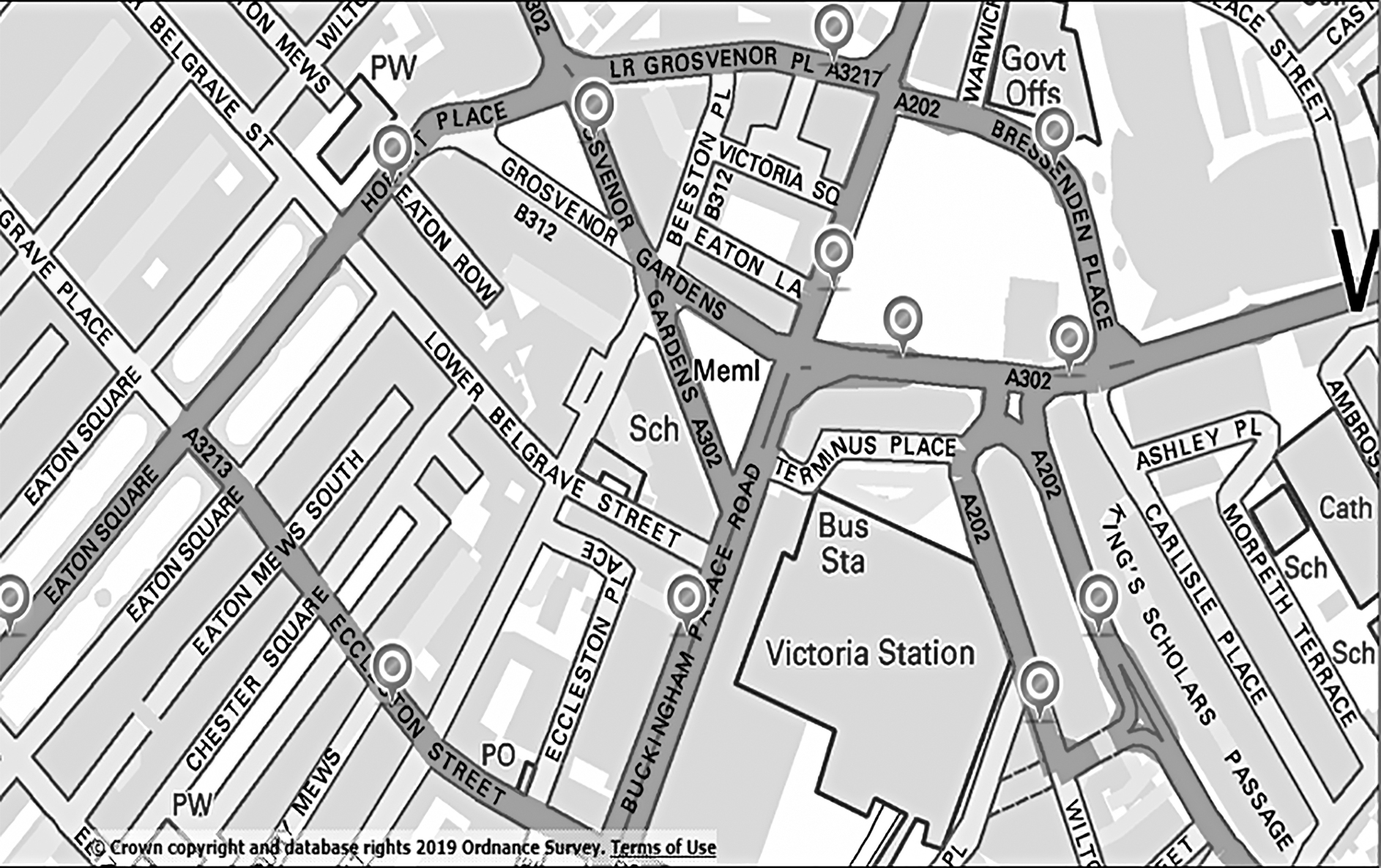
Partial map showing various count points.

FIG. 4.

Map plot of data points in the data set.

Data set 2: PEMS-SF data set

The second data set is taken from PEMS-SF⁴¹ that exhibits multivariate characteristics. It consists of a total of 440 instances and 138,672 attributes that have real characteristics. The proposed CDE-Fuzzy DBN model is given to the data collected from the Caltrans Performance Measurement System (PEMS) database. Marco Cuturi, who is the creator of the data set, has downloaded data from the California Department of Transportation PEMS website for 15 months (January 1, 2008, to March 30, 2009), illustrating the occupancy rate of various car lanes in the San Francisco bay area. The data collected in an interval of 10 minutes, considering every day as a single time series data having dimension 963 with span 6 × 24 = 144. Excluding the data on all the public holidays, the database contains 440 time series data. Hence, the database includes 963 × 144 = 138.672 attributes for every data record. Similar to data set 1, here too, the experiment is carried out by considering 70% of samples for training and the remaining for testing on an incremental basis.

Performance index

To evaluate the performance of the proposed technique, we use two performance indexes, which are the log mean square error (LMSE) and the log root mean square error (LRMSE).

Log mean square error

Mean square error (MSE) is based on the average of the error between the observed value and the predicted output of the classifier from the classifier. The formula for the MSE is updated in Equation (37), with LMSE,⁴² obtained by taking the log of the MSE. $L M S E = log [{\in^{1}}_{a v g}] = log [\frac{1}{ℜ} {\sum_{x = 1}^{ℜ} (O_{q} - g)}^{2}],$ (37)

where O_q is the actual output, g is the expected output, and $ℜ$ is the total number of samples.

Log root mean square error

Root mean square error (RMSE) is defined as the measure of the observed values and the predicted values. The RMSE is the square root of MSE, and the LRMSE⁴³ is computed as the log of the RMSE value as shown in Equation (38). $L R M S E = log [\sqrt{\frac{1}{ℜ} {\sum_{x = 1}^{ℜ} (O_{q} - g)}^{2}}],$ (38)

where O_q is the actual output, g is the expected output, and $ℜ$ is the total number of samples.

Relative error

The relative error of two methods is the absolute value of the error between the methods. The significance of using relative error is to specify the percent improvement of the proposed method when compared with the existing methods. The relative error of $i t h$ method with respect to $j t h$ method is computed as $R E = \frac{|E R R O R_{i} - E R R O R_{j}|}{max (|E R R O R_{i}, E R R O R_{j}|)} \times 100,$ (39)

where $E R R O R_{i}$ and $E R R O R_{j}$ refer to the LMSE/LRMSE values of the $i t h$ and $j t h$ methods, respectively.

Comparative methods

The methods used for analysis include DBN,¹¹ Deep Network using Autoencoder,⁸ Wavelet NN,¹⁷ NARX LM,¹⁸ RNN,²² KNN-LSTM network,²³ and CDE-Fuzzy DBN without technical indicators, and the results of the existing methods are compared with the proposed CDE-Fuzzy DBN method of TFP.

Comparative analysis

This section demonstrates the comparative analysis using two data sets based on LMSE and LRMSE with respect to the time steps in either years or interval of 5 minutes. Totally, three sets of analysis are carried out through varying the number of hidden layers as 1, 2, and 3, respectively, using the two data sets. While analyzing the performance of each set, the best performance has been obtained using three hidden layers, which is provided in this section.

Analysis based on data set 1

The analysis using the data set 1 is discussed based on the performance metrics and the time step duration given in years for long-term TFP.

With the number of hidden layers = 3

Figure 5 shows the analysis for all vehicle types in terms of LMSE and LRMSE using three hidden layers. Figure 5a shows the analysis using LMSE. The LMSE values for the methods CDE-Fuzzy DBN, DBN, Wavelet NN, NARX-LM, Deep Network using Autoencoder, RNN, KNN-LSTM, and CDE-Fuzzy DBN without technical indicators when the time step duration is 1 year are 2.4141, 3.5755, 3.8373, 3.2980, 3.0998, 2.9506, 3.7296, and 2.6254, respectively. In the fifth year, the value of LMSE for CDE-Fuzzy DBN, DBN, Wavelet NN, NARX-LM, Deep Network using Autoencoder, RNN, KNN-LSTM, and CDE-Fuzzy DBN without technical indicators are 2.4815, 3.6908, 3.9594, 3.3969, 3.0614, 3.0387, 3.5996, and 2.6136, respectively. It is observed that CDE-Fuzzy DBN has a low value of LMSE compared with the existing methods.

FIG. 5.

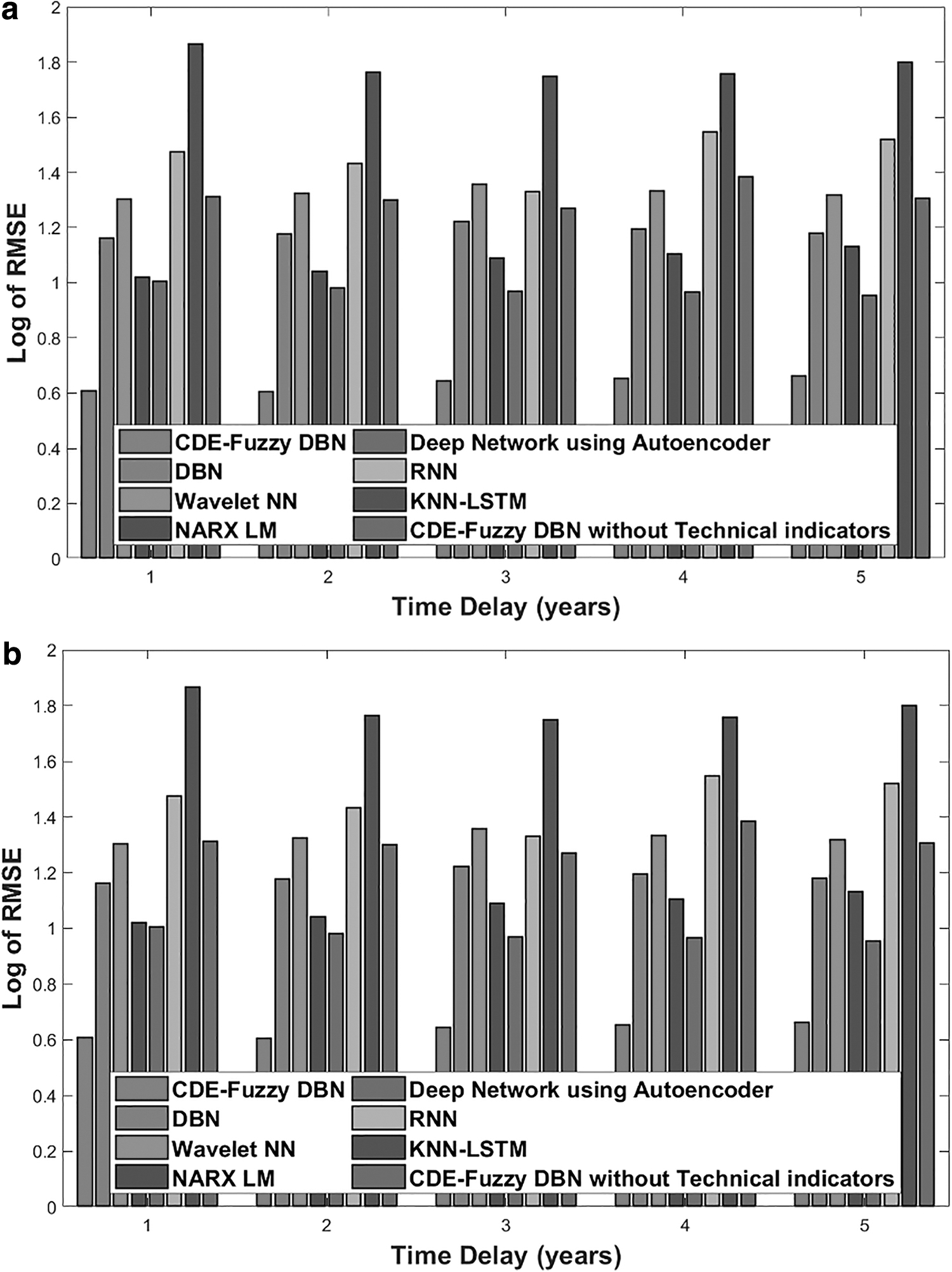
Performance analysis using three hidden layers. (a) Time interval in years versus LMSE. (b) Time interval in years versus LRMSE. LMSE, log mean square error; LRMSE, log root mean square error.

It is observed that CDE-Fuzzy DBN has a low value of LMSE compared with the existing methods. Figure 5b depicts the comparative analysis in terms of LRMSE for all vehicles with three hidden layers. The relative error of CDE-Fuzzy DBN with respect to DBN, Wavelet NN, NARX-LM, Deep Network using Autoencoder, RNN, KNN-LSTM, and CDE-Fuzzy DBN without technical indicators are 47.5%, 53.16%, 40.20%, 39.45%, 58.65%, 67.29% and 53.53%, respectively, when the interval is 1 year.

Analysis based on data set 2

The analysis using data set 2 is demonstrated in this section, and the time step interval is 5 minutes for short-term TFP.

With number of hidden layers = 3

Figure 6 shows the analysis using PEMS data in terms of LMSE and LRMSE using three hidden layers. The analysis of LMSE is enumerated in Figure 6a that demonstrates the variance of LMSE for the time step intervals of 5, 10, 15, 20, and 25 minutes. The LMSE of the methods is found to be decreasing upon an increase in the time duration from 5 to 25 minutes. The LMSE for CDE-Fuzzy DBN at the interval of 5 minutes is 1.6690 and 1.7178 at the interval of 25 minutes represents that the method makes effective results. Additionally, the second-best classifier that offers less LMSE is the CDE-Fuzzy DBN without technical indicators, offering LMSE of 1.8745 at the interval of 5 minutes and 1.7496 at the interval of 25 minutes. The relative error of CDE-Fuzzy DBN is 20.78% with the DBN and 66.29% with the wavelet NN for interval of 25 minutes. Figure 6b depicts the comparative analysis based on the LRMSE. The LRMSE values of CDE-Fuzzy DBN, DBN, Wavelet NN, NARX-LM, Deep Network using Autoencoder, RNN, KNN-LSTM, and CDE-Fuzzy DBN without technical indicators are 0.5456, 0.7801, 1.5275, 1.3147, 1.1293, 1.2363, 1.9192, and 0.8748, respectively, when the interval is 25 minutes. The graph makes it clear that the CDE-Fuzzy DBN acquires a less value of LRMSE for all the intervals when compared with the existing methods.

FIG. 6.

Performance analysis using three hidden layers. (a) Time step interval of 5 minutes versus LMSE. (b) Time step interval of 5 minutes versus LRMSE.

Comparative discussion

Table 2 shows the analysis of the TFP methods using data set 1 and data set 2 based on the best performance values obtained by the comparative methods. The analysis using the instances for both the data sets depicts useful information. It can be observed that the proposed method CDE-Fuzzy DBN outperforms rest of the techniques due to the technical indicators and optimization method used. CDE-Fuzzy DBN without technical indicators shows the second best results for the metrics LMSE and LRMSE. From Table 2, it is depicted that the proposed CDE-Fuzzy DBN acquired a minimum value of LMSE and LRMSE for both the data sets.

Table 2.

Comparative analysis of the prediction methods using data set 1 and data set 2

Metrics	CDE-Fuzzy DBN	DBN	Wavelet NN	NARX-LM	Deep network using Autoencoder	RNN	KNN-LSTM	CDE-Fuzzy DBN without technical indicators
Data set 1
LMSE	2.4141	3.5755	3.8373	3.2981	3.0999	2.9506	3.7296	2.6254
LRMSE	0.6100	1.1620	1.3025	1.0202	1.0075	1.4753	1.8648	1.3127
Data set 2
LMSE	1.6691	2.2233	4.5841	3.7860	2.7818	2.0971	2.9857	1.8745
LRMSE	0.5208	0.8213	1.4375	1.3681	1.0899	1.0485	1.4928	0.9373

LMSE, log mean square error; LRMSE, log root mean square error.

Conclusion

We propose a DL approach with technical indicators, fuzzy membership functions, and bioinspired optimization algorithm over DBN for TFP. Unlike existing techniques, which utilize shallow methods, our proposed TFP method uses an incremental CDE-Fuzzy-optimization-based DBN reliable for long-term and short-term TFP consisting of huge set of nonlinear data. The usage of technical indicators adds value to the work as it is capable of dealing with the nonlinear spatial and temporal correlation from the traffic data, which is incremental in nature. The prediction involved two major steps: In the first step, we applied the indicators to extract the flow strength features using MOM, RSI, CCI, ADX, and TEMA, and in the second step, the traffic flow is predicted using the DBN classifier, trained using the CDE-Fuzzy algorithm. The optimal weights for the DBN are computed using the CDE-Fuzzy algorithm, modeled by incorporating the fuzzy concepts in the DE algorithm. The experimental analysis performed on standard data set shows that the proposed CDE-Fuzzy DBN model outperforms the rest by solving uncertainty of nonlinearity in traffic flow data. The results obtained by the proposed method guarantee accurate traffic management in ITS. For future work, it will be interesting to investigate an improvement over DL with hybrid method and utilize the concept for transfer learning to predict the traffic flow in homogenous spatial links with inadequate data.

Footnotes

Author Disclosure Statement

No competing financial interests exist.

Funding Information

No funding was received.

Abbreviations Used

References

Zhao

, Su

. High-order Gaussian process dynamical models for traffic flow prediction. IEEE Trans Intell Transp Syst, 2016; 17:2014–2019.

, Zhu

, Wu

G-Q

, Ding

. Data mining with big data. IEEE Trans Knowl Data Eng, 2014; 26:97–107.

Shi

, Abdel-Aty

. Big data applications in real-time traffic operation and safety monitoring and improvement on urban expressways. Transp Res Part C Emerg Technol, 2015; 58:380–394.

Dell'Acqua

, Bellotti

, Berta

, et al. Time-aware multivariate nearest neighbor regression methods for traffic flow prediction. IEEE Trans Intell Transp Syst, 2015; 16:3393–3402.

Roess

, Prassas

, McShane

. Traffic Engineering, 4th ed. Upper Saddle River, NJ: Prentice-Hall, 2010.

Zhang

, Wang

F-Y

, Zhu

, et al. DynaCAS: Computational experiments and decision support for ITS. IEEE Intell Syst, 2008; 23:19–23.

Ahn

, Ko

, Kim

. Highway traffic flow prediction using support vector regression and Bayesian classifier. In: Proceedings of the International Conference on Big Data and Smart Computing (BigComp). Hong Kong, China, 2016, pp. 239–244.

, Duan

, Kang

, et al. Traffic flow prediction with big data: A deep learning approach. IEEE Trans Intell Transp Syst, 2015; 16:865–873.

Xia

, Li

, Wang

, et al. A map reduce-based nearest neighbor approach for Big-Data-driven traffic flow prediction. IEEE Access, 2016; 4:2920–2934.

10.

, Wen

, Chua

T-S

, et al. Toward scalable systems for big data analytics: A technology tutorial. IEEE Access, 2014; 2:652–687.

11.

Huang

, Song

, Hong

, et al. Deep architecture for traffic flow prediction: Deep belief networks with multitask learning. IEEE Trans Intell Transp Syst, 2014; 15:2191–2201.

12.

, Jiang

, Zhu

, et al. Multiple measures-based chaotic time series for traffic flow prediction based on Bayesian theory. Nonlinear Dyn, 2016; 85:179–194.

13.

Wibisono

, Jatmiko

, Wisesa

, et al. Traffic big data prediction and visualization using fast incremental model trees-drift detection (FIMT-DD). Knowl Based Syst, 2012; 93:33–46.

14.

, Yan

, Liu

, et al. A short-term traffic flow forecasting method based on the hybrid PSO-SVR. Neural Process Lett, 2016; 43:155–172.

15.

S-D

, Kim

Y-J

, Hong

J-S

. Urban traffic flow prediction system using a multifactor pattern recognition model. IEEE Trans Intell Transp Syst, 2015; 16:2744–2755.

16.

Vasantha Kumar

, Vanajakshi

. Short-term traffic flow prediction using seasonal ARIMA model with limited input data. Eur Transp Res Rev, 2015; 7:1–9.

17.

Yanchong

, Darong

, Ling

A short-term traffic flow prediction method based on wavelet analysis and neural network. In: Proceedings of the Chinese Control and Decision Conference (CCDC). Yinchuan, China, 2016, pp. 7030–1034.

18.

Banjanović-Mehmedović

, Butigan

, Kantardžić

, et al. Prediction of cooperative platooning maneuvers using NARX neural network. In: Proceedings of the International Conference on Smart Systems and Technologies (SST). Osijek, Croatia, 2016, pp. 287–292.

19.

Koesdwiady

, Soua

, Karray

. Improving traffic flow prediction with weather information in connected cars: A deep learning approach. IEEE Trans Veh Technol, 2016; 65:9508–9517.

20.

Yang

H-F

, Dillon

, Chen

PY-P

. Optimized structure of the traffic flow forecasting model with a deep learning approach. IEEE Trans Neural Netw Learn Syst, 2017; 28:2371–2381.

21.

Jia

, Wu

, Ben-Akiva

, et al. Rainfall-integrated traffic speed prediction using deep learning method. IET Intell Transp Syst, 2017; 11:531–536.

22.

Tian

, Pan

Predicting short-term traffic flow by long short-term memory recurrent neural network. In: Proceedings of IEEE International Conference on Smart City/SocialCom/SustainCom together with DataCom. Chengdu, China, 2015, pp. 153–158.

23.

Luo

, Li

, Yang

, et al. Spatiotemporal traffic flow prediction with KNN and LSTM. J Adv Transp, 2019; 2019:1–10.

24.

Abdi

, Moshiri

, Abdulhai

, et al. Short-term traffic flow forecasting: Parametric and nonparametric approaches via emotional temporal difference learning. Neural Comput Appl, 2013; 23:141–159.

25.

George

, Santra

. Deep learning techniques for traffic flow prediction in intelligent transportation system: A survey. Test Eng Manage, 2020; 82:9773–9789.

26.

Duan

, Yang

, Zhang

, et al. Improved deep hybrid networks for urban traffic flow prediction using trajectory data. IEEE Access, 2018; 6:31820–31827.

27.

Zheng

, Yang

, Liu

, et al. Deep and embedded learning approach for traffic flow prediction in urban informatics. IEEE Trans Intell Transp Syst, 2019; 20:3927–3939.

28.

, Yu

, Wang

, et al. Large-scale transportation network congestion evolution prediction using deep learning theory. PLoS One, 2015; 10: e0119044.

29.

Yang

H-F

, Dillon

, Chen

PY-P

. Optimized structure of the traffic flow forecasting model with a deep learning approach. IEEE Trans Neural Netw Learn Syst, 2017; 28:2371–2381.

30.

Bengio

Learning deep architectures for AI, vol. 2. Foundations and Trends^® in Machine Learning 2009, pp. 1–127.

31.

Hinton

, Salakhutdinov

. Reducing the dimensionality of data with neural networks. Science, 2006; 313:504–507.

32.

Stock Trend Prediction with Technical Indicators using SVM. Stanford, CA: Stanford University, 2014.

33.

Oriani

, Coelho

. Evaluating the impact of technical indicators on stock forecasting. In: 2016 IEEE Symposium Series on Computational Intelligence (SSCI). Athens 2016, pp. 1–8.

34.

Vigos

, Papageorgiou

. A simplified estimation scheme for the number of vehicles in signalized links. IEEE Trans Intell Transp Syst, 2010; 11:312–321.

35.

Borkar

, Mahajan

. A secure and trust based on-demand multipath routing scheme for self-organized mobile ad-hoc networks. Wireless Netw, 2017; 23:2455–2472.

36.

George

, Santra

. An improved long short-term memory networks with Takagi-Sugeno fuzzy for traffic speed prediction considering abnormal traffic situation. Comput Intell, 2020; [Epub ahead of print]: DOI: 10.1111/coin.12291.

37.

Rommelfanger

The advantages of fuzzy optimization models in practical use. Fuzzy Optim Decis Making, 2004; 3:295–309.

38.

Dennis

, Muthukrishnan

. AGFS: Adaptive Genetic Fuzzy System for medical data classification. Appl Soft Comput, 2014; 25:242–252.

39.

Liu

, Wang

, Liu

. A survey of deep neural network architectures and their applications. Neurocomputing, 2017; 234:11–26.

40.

Traffic-major roads (km). Available online at https://data.gov.uk/dataset/gb-road-traffic-counts (last accessed December 2017 ).

41.

PEMS-SF Data Set. UCI Machine Learning Repository. Available online at https://archive.ics.uci.edu/ml/datasets/PEMS-SF (last accessed November 2018 ).

42.

Thompson

PA.

Evaluation of the M-competition forecasts via log mean squared error ratio. Int J Forecast, 1991; 7:331–334.

43.

Carlisle

Digital Elevation Model Quality and Uncertainty in DEM-based Spatial Modelling. London, United Kingdom: University of Greenwich, 2002.