A Convolutional Neural Network to Perform Object Detection and Identification in Visual Large-Scale Data

Abstract

In recent years, big data became a hard challenge. Analyzing big data needs a lot of speed precision combination. In this article, we describe a deep learning-based method to deal with big data with a focus on precision and speed. In our case, the data are images that are the hardest type of data to manipulate because of their complex structure that needs a lot of computation power. Besides, we will solve a hard task on images, which is object detection and identification. Thus, every object in the image will be localized and classified according to the range of classes provided by the training data set. To solve this challenge, we propose an approach based on a deep convolutional neural network (CNN). Moreover, CNN is the most used deep learning model in computer vision tasks such as image classification and object recognition because of its power in self-features extraction and provides useful techniques in the prediction of decision-making. Our approach outperforms state-of-the-art models such as R-CNN, Fast R-CNN, Faster R-CNN, and YOLO (you only look once), with 77% of mean average precision on the Pascal_voc 2007 testing data set and a speed of 16.54 FPS using an Nvidia Geforce GTX 960 GPGPU.

Introduction

For a human, processing an image is a straightforward and fast task. One glance allows the human being to analyze an image and extract all relevant information from it. Also, a human can manipulate a significant amount of visual data at the same time because the human brain is a very complex processing unit¹ that still until now a vague phenomenon.

The brain is the central unit in the nervous system and the control unit of the body. It is composed of a very complicated neural network² connected to provide a brilliant system to make predictions and decisions based mainly on visual information provided by the eyes. The processing way that the human brain use is very misty, but researchers somehow introduce a mathematical and informatic representation of the biological neural of the human brain called an artificial neuron. Researchers presented a similar technique to the brain workflow to process data in computer vision tasks called “deep learning.”

Deep learning is an artificial intelligence technique that gives computers the ability to learn from examples based on a deep artificial neural network simulated from the human brain architecture. The main goal is to mimic brain methodology in processing data and decision-making. In recent years, the deep learning techniques achieve great success in solving a wide range of artificial intelligence applications because of its ability of features self-extraction without the need of the handcrafted features engineering. Deep learning techniques make it possible to learn directly from the data and eliminate the feature extraction process imposed by the old machine learning techniques. In addition, those techniques show considerable success in solving hard challenges in many fields, such as computer vision³ and natural language processing.⁴ In our case, we will address a challenge in the computer vision field, which is object detection and identification.

The most known deep learning model to solve computer vision tasks is the convolutional neural network (CNN).⁵ It was deployed in object recognition and image classification tasks with success. The most important reasons that make CNNs works are their architecture and the importance of the convolution function that allows to extract handy features from the image and generating a unique representation of each pattern in the image. Also, the final layers will enable the extraction of global features and combine them with the extracted local features to provide useful predictions. CNN are feedforward networks that allow improving the speed and precision combination.

In this work, a CNN architecture will be introduced to deal with a complex task, which is object detection and identification. First, object detection aims to localize each object in the image. The network output is a vector that will provide the coordination of the localization box, so a regression task must be solved. Second, the object identification task aims to classify the localized objects in the image. So, the network output will be the class of the object, and this will be solved as a classification task. The object detection and identification will be applied to big data, which is a data set with a vast amount of data. In our case, the data are images.

The remainder of the article is organized as follows. Related works on object detection and identification are presented in the Related Works section. The Convolutional Neural Networks section discusses the CNN architecture and its fundamental theory. The big data and the data sets used in the training and testing process are introduced in the Digital Large-Scale Data section. The Proposed Approach section describes the proposed approach and how it works. In the Experiment and Results section, experiments, results, and comparison against the state-of-the-art models are detailed. Finally, the Conclusion section concludes the article.

Related Works

In the object detection or identification task, we can find a lot of methods, especially those based on deep learning techniques. The most known technique for object detection task are the region proposal methods. Grouping superpixels is the basis of the region proposal methods, such as selective search,⁶ the Constrained Parametric Min-Cuts,⁷ and the Multiscale Combinatorial Grouping.⁸ Also, some other methods based on sliding windows such as the Edge boxes⁸ and the objectness in windows⁹ were used. All the mentioned methods are external modules connected to the network used for the detector and that causes a slow processing time since they generate arbitrary regions that need a lot of processing time to provide a prediction on all the proposed regions. Those region proposal methods are used in several works, such as R-CNN,¹⁰ SPP Net,¹¹ and fast R-CNN.¹²

Also, we can find some deep neural networks for region proposal and bounding boxes prediction works. The Overfeat¹³ model is based on a trainable fully connected layer to predict bounding box parameters: x,y coordinates, height, and width. To generate a bounding box, they simultaneously run a classifier and a regressor network on all locations and scales. Since the extracted features are shared between the networks, they need to reproduce the final regression layer after performing the classification process, this method can only predict multiple unique object class. Other methods such as the Multibox methods^14,15 allow generating region proposal from a network. The Multibox methods can generate multiclass objects bounding boxes. Those methods do not share the extracted features between classification and region proposal networks. Deep Mask¹⁶ method was used for segmentation proposals. Most of the shared convolutional features methods^13–16 have been developed to enhance CNN accuracy and efficiency in visual object detection tasks. The fast R-CNN model¹² introduces an end-to-end training detector based on shared convolutional features and achieves excellent performance.

Another breakthrough benchmark in the object detection task is faster R-CNN.¹⁷ It was a combination of tow convolutional networks. The first is fully CNN¹⁸ for region proposal and the second is a traditional CNN such as VGG Net¹⁹ and ZFNet²⁰ for the classification. YOLO²¹ as they named (you only look once) introduce a single pipeline to perform the detection problem. It uses an end-to-end CNN and solves the detection task as a regression problem. So, the bounding box coordinates and the class are determined at the same time.

For the object identification task, there are several works based on CNNs²² such as the famous AlexNet.²³ It was a CNN that wins the image net large-scale visual recognition challenge ILSVRC 2012.^24,25 AlexNet achieves a 15.43% top 5 error in the image classification task surpassing the second competitor with more than 10%. Also, GoogleNet²⁶ was a well-known benchmark in the image classification task. It wins the ILSVRC 2014 object classification and detection task, and it reduces the top 5 errors to 6.54% and achieves a mean average precision (AP) in the detection task of 43.93%. Also, the ResNet model,²⁷ a profound CNN with 152 layers of depth. It reduces the top 5 errors to 3.52% in the classification task.

Convolutional Neural Networks

CNN is an artificial neural network model introduced by Fukushima²⁸ in 1980 and have been enhanced by LeCun²⁹ in 1998 for computer vision tasks, such as object recognition and detection.

CNN is a feedforward neural network used for supervised learning. CNN is composed of six layers types. An input layer which is an image, a convolutional layer for feature extraction generally flowed by a nonlinear layer used to avoid neurons saturation and to make neuron responses robust to data corruption. A pooling layer to reduce the feature map dimensions to make them less susceptible to input distortion and to reduce the parameter number manipulated in the final layers because smaller feature maps generate fewer parameters and help to avoid network complexity and the overfitting problem. A fully connected layer to extract global features and to combine the extracted local features. An output layer to provide predictions.

In computer vision tasks, CNN achieves state-of-the-art performance because the biological system inspired it. As shown in Figure 1, hidden neurons of a CNN are just connected to a local patch in the previous layer called filter where each filter (cell) is sensitive to a small region in the input image called the receptive field. Each receptive field can be considered as a detector for a particular visual pattern. Then, many cells are correlated together to cover the whole visual field. So, a hidden neuron in each location can share the same weights with other neurons, and the number of the learned parameters will be reduced.

FIG. 1.

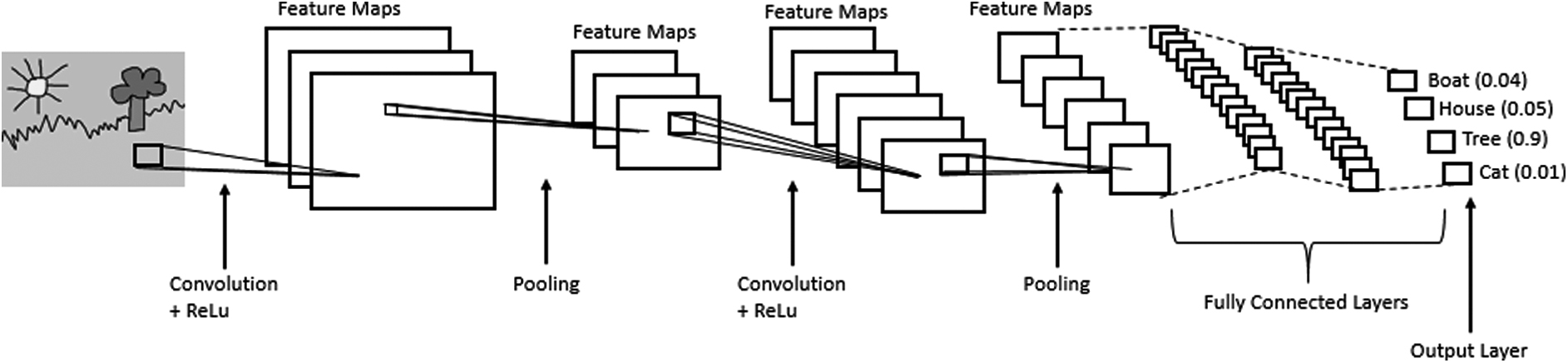
Convolutional neural network.

The input layer is generally a color image with a red green blue (RGB) space color. The convolutional layer is generated by the result of the sum of the convolution between an input layer $n_{1}^{k}$ and three-dimensional filter (height, width, and depth) bank $w_{i j}^{k}$ and a trainable bias term $b_{j}^{k}$ . A neuron in the convolutional layer can be calculated as Equation (1) and * denotes the two-dimensional (2D) convolution operation. $y_{j}^{k} = \sum_{i} (x_{i}^{k} * w_{i j}^{k}) + b_{j}^{k}$ (1)

A demonstration of the convolution process is illustrated in Figure 2. The nonlinear layer is a nonlinear activation function applied to the previous layers. For the nonlinear function, the sigmoid or the rectified linear unit (ReLU) is the most used. In 2012, Hinton and colleagues²³ proved that using the ReLU as an activation function is better than other activation functions because it generates robust neuron responses to data corruption. So, if the input image is damaged, it will not generate negative results in the output feature map. Assuming that ReLU is a nonlinear function, the output of this layer can be computed as Equation (2).

FIG. 2.

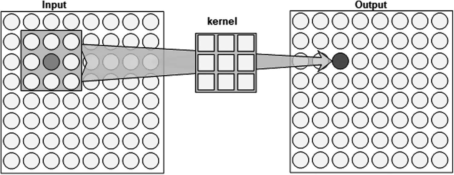
Convolution process.

ỹ_{j}^{k} = m a x (0, y_{j}^{k})

(2)

The pooling layer is used to compress feature maps and for dimension reduction. This layer is used to reduce the sensitivity of the output feature maps because of the input feature map distortion. In addition, small feature maps provide fewer parameters to manipulate, resulting in less network complexity and speed up the training and testing processes. Also, the pooling layer is used to detect all patterns in the image, whatever its location in the input image. The commonly used pooling functions are the max pooling and the average pooling. Thus, a nonoverlapped neurons neighborhood in a feature map can be replaced by the maximal or the average neuron of those neurons.

According to the number of filters used, a number of the feature maps were generated in the hidden layer. The dimension of a hidden layer depends on the kernel size and the stride used to slide the kernel across the feature map. After several convolutions, nonlinear and pooling layers according to the depth of the network, fully connected layers were added. A fully connected layer is a vector that contains all the feature maps of the previous layer where every neuron of this layer is connected to all the neurons of the previous layer. The fully connected layer is a vectorial representation of the extracted features. So, the local features are learned in the bottom layers and the global features are extracted in the high-level layers. To generate the output, a fully connected layer dotted with normalized exponential (Softmax) was used for the classification problem and the linear regression function for the regression problem. The number of neurons in the output layer represents the number of classes for the multiclassification problem and the probability of each class is calculated as Equation (3). For the regression, the number of neurons represents the parameters to predict and the linear regression can be calculated as Equation (4). $p (y_{j} | x) = \frac{e^{x^{T} w_{j}}}{\sum_{i = 1}^{k} e^{x^{T} w_{i}}}$ (3)

y = a x + b

(4)

a = \frac{n (\sum_{i = 0}^{n} x_{i} y_{i}) - (\sum_{i = 0}^{n} x_{i}) (\sum_{i = 0}^{n} y_{i})}{n (\sum_{i = 0}^{n} x_{i}^{2}) - {(\sum_{i = 0}^{n} x_{i})}^{2}}

b = \frac{(\sum_{i = 0}^{n} y_{i}) - a (\sum_{i = 0}^{n} x_{i})}{n}

Digital Large-Scale Data

Large-scale data is a data set with a huge amount of digital data with a complex structure that is hard to manipulate.³⁰ Nowadays, big data exists everywhere and can be used in different domains. The big main data challenges are data computing, data storage in servers for numerical research using search engines, visualization such as in video surveillance analyses, and so on. Usually, large-scale data cannot be manipulated using traditional software because of its size beyond the ability of those commonly used software tools generally used for managing and processing data with the speed and precision needed.³¹ Big data can be structured, semi-structured, or unstructured data,³² and the hardest task is how to manage unstructured data.

In 2012, big data size achieves a big explosion to attend some petabytes of data.³³ Big data needs a new set of techniques to deal with the diverse, complex, and massive data scale.³⁴ The deep learning techniques allow manipulating big data with a focus on precision and speed. Deep learning algorithms are based on deep artificial neural networks, such as CNNs and deep belief networks.

In this work, the data are images, and to deal with images, the most commonly used deep learning model is the CNNs because of their similarity to the human biological system in data processing and decision-making. This work aims to analyze images to detect objects and identify them in large-scale data sets. To perform this task, a combination of speed and precision is needed. However, building a well-performed algorithm for object detection was and still a hard challenge. Objects in the image present some unbalanced varieties, such as color variety, size variety, shape variety, and occlusion. Also, the same object presents a variety of challenges that must be handled like the change of the point of view, orientation, and deformation. To deal with all those challenges, the deep learning technique was deployed successfully because of their robustness in a wide range of challenges, such as object recognition and image classification. Moreover, deep learning algorithms need large-scale data to raise their performance.

Deep learning algorithms are machine learning algorithms based on neural networks and need a considerable amount of data to learn. As a result, big data and deep learning are strongly connected. Deep learning needs big data to learn, and deep learning was required to deal with significant big data challenges. For the moment, a lot of large-scale data sets are available and can be used to train or evaluate deep learning models to determine their performance. For object detection in significant data challenges, several data sets can be used.

Pascal voc (Pattern analysis, statistical modeling, and computational learning visual objects classes challenge) data set³⁵ is a free large-scale data set founded in 2005 by a combination of universities for a wide range of challenges, such as object classification, object detection, and object segmentation. For object detection, the most commonly used are Pascal_voc 2007 and Pascal_voc 2012. The Pascal_voc 2007 contains 9963 images from 20 classes with 24,640 annotated objects. The Pascal_voc 2012 contains 11,530 images from 20 classes with 27,450 annotated objects.

Also, the COCO (common object in context)³⁶ is a large-scale data set for object detection, object classification, and object segmentation tasks. COCO is founded by Microsoft research laboratory. It contains 330,000 images, more than 200,000 images are labeled, from 80 class with 1.5 million object instances. An image in COCO data set can contain five captions.

The ImageNet²⁵ is a very large-scale data set introduced by Google research laboratory. It can be used for a wide range of challenges, such as image classification and object detection. For object detection task, ImageNet has 456,182 images from 200 class with 401,356 annotated objects. Each data set from the mentioned data sets contains separated training data and testing data.

Proposed Approach

The proposed approach was inspired by existing architecture with some improvements. It was specified for handling one of the hardest tasks, which are detecting and identifying objects in real images in the most complex challenges: the big data, one of the most important challenges that push technology innovation. Big data exists everywhere, in social media, websites, medicine and surveillance systems, and so on.

To solve a big data challenge, high performance was needed. This architecture was designed to offer a balanced performance by proving both accuracy and speed. All existing architectures are proved in one-way performance either accuracy or speed. For example, the R-CNN family was designed for accuracy and the YOLO family was designed for speed.

The proposed architecture is based on a CNN with two outputs: a classification head and a regression head. The regression head will be used to detect objects and localize them in the image. The classification head will be used to identify objects that means that it will provide the class of each detected object in the image. As an output of the regression head, the x,y coordinates, the height, and the width of the bounding box will be determined. An illustration of an image as an output of our approach is shown in Figure 3. As an input of the CNN, RGB space color images were injected. The input image can take any size and then it will be resized. The minimal size will be 600 pixels and the maximum size will be 1000 pixels so an optimal image has a size of 600 × 1000 × 3, 3 denotes the RGB space color. The input image was resized to achieve a balance between speed and accuracy. The proposed size maintains the high resolution of the image and allows achieving accepted processing time since larger images result in slower processing time and small images result in losing important features and degrading the accuracy.

FIG. 3.

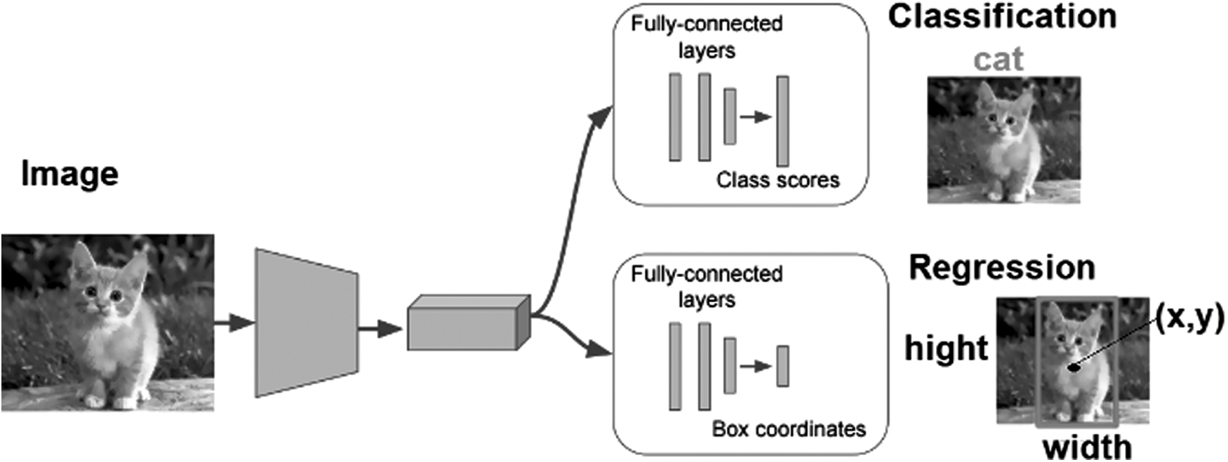
Classification and regression using the same network.

The main focus was to achieve a trade-off between speed and accuracy. In effect, using a big number of hidden layers will increase the processing time, and using a few hidden layers will decrease the accuracy. So, a CNN (Convnet) was proposed. The Convnet was composed of 13 convolutional layers. Thirteen nonlinear layers (CONV for Convolutional + nonlinear) and four pooling layers (POOL). The pooling layers are flowing the 2nd, the 4th, the 7th, and the 10th convolutional layers, as shown in Figure 4. A stride of 1 was fixed to slide the filters across the convolutional layers and a stride of 2 was fixed for the pooling layers of the Convnet. Also, the kernel size of the filters was fixed as 3 × 3 for convolutional and pooling layers. Starting with 64 2D filters for the first two convolutional layers (CONV1 and CONV2). Then, the number of 2D filters for the convolutional layers was doubled after each pooling layer except for the last three convolutional layers after the POOL4 layer. Table 1 summarizes the different parameters of the Convnet layers. For the abbreviations, #F refers to the number of applied filters, #IFM refers to the number of the input feature maps, and #OFM refers to the number of the output feature maps. The ReLU was used for the nonlinear layers. A Max-Pooling function was chosen for the pooling layers. Also, we apply zero paddings with all the pooling layers.

FIG. 4.

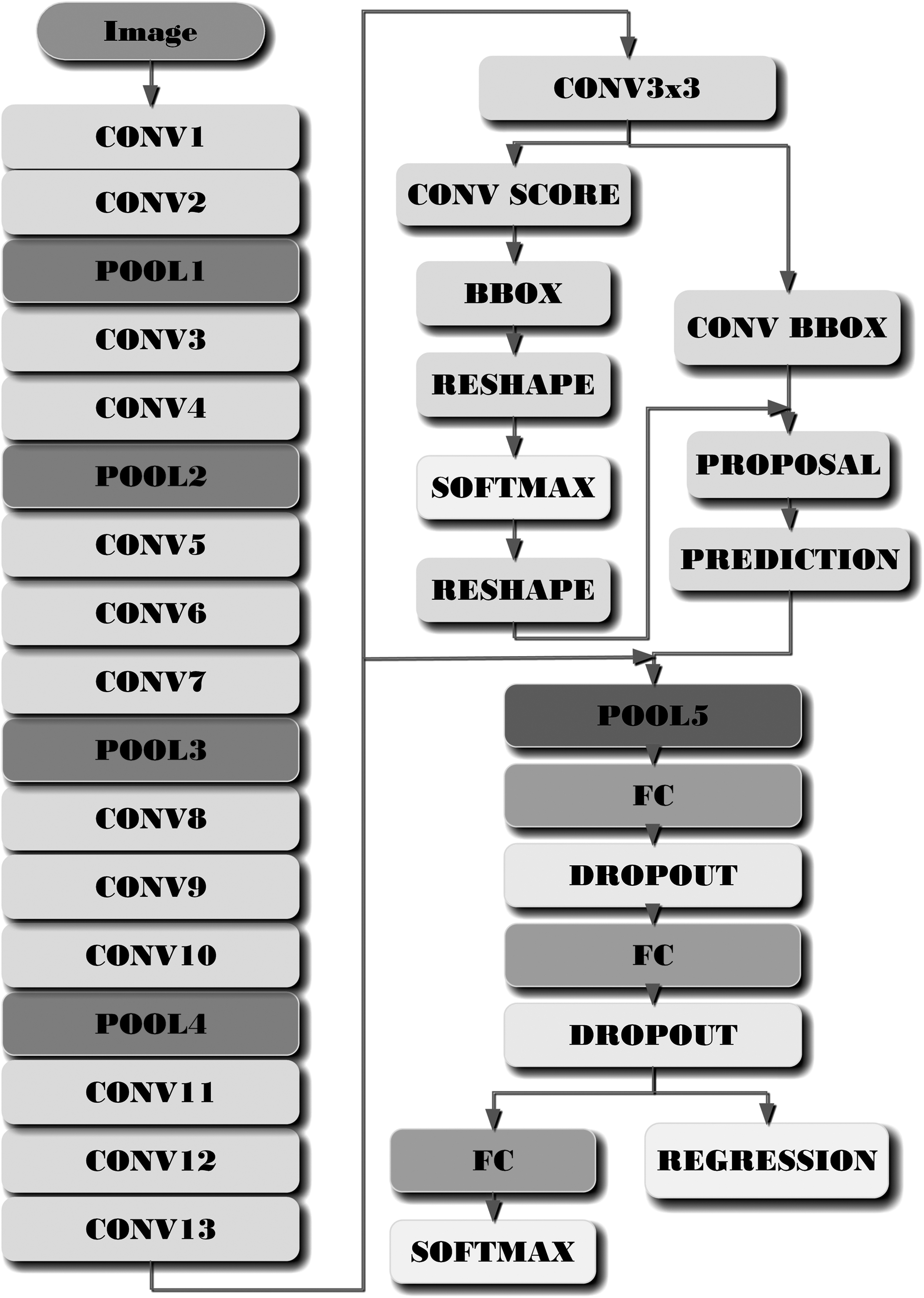
Proposed convolutional neural network model for object detection and identification.

Table 1.

Parameters of the Convnet layers

Layer	#F	#IFM	#OFM
INPUT	—	3	3
CONV1	64	3	64
CONV2	64	64	64
POOL1	64	64	64
CONV3	128	64	128
CONV4	128	128	128
POOL2	128	128	128
CONV5	256	128	256
CONV6	256	256	256
CONV7	256	256	256
POOL3	256	256	256
CONV8	256	512	512
CONV9	512	512	512
CONV10	512	512	512
POOL4	512	512	512
CONV11	512	512	512
CONV12	512	512	512
CONV13	512	512	512

#F, the number of applied filters; #IFM, the number of the input feature maps; #OFM, the number of the output feature maps.

To generate region proposals, a CNN connected to the last convolutional feature maps of the Convnet was used. Then, we apply a 3 × 3 sliding window across this feature map, followed by a 1 × 1 convolutional layer for binary classification (CONV SCORE) and another convolutional layer for localization to generate proposals regions (CONV BBOX).

Each selected window was tested if there is an object or not using a Softmax layer. To determine if the selected region contains an object or not, we apply nine different bounding boxes scales, as presented in Table 2. A projection on the input image was performed, then the intersection over union (IoU) factor was calculated as Equation (5). The IoU is the intersection area between the bounding box (light gray in Fig. 5) and the ground truth provided by the training sets (dark gray in Fig. 5) over the union area of the same boxes. As configuration if the IoU value is less than 0.3 so the selected region does not contain an object and if the IoU value is more than 0.7 so the selected region contains an object. The bounding box parameters provided are used to generate proposed regions and send them to the detector to fine-tune the position of the bounding box and its dimension. Also, the proposed region will be sent to the classier to identify the object.

FIG. 5.

IoU calculation. IoU, intersection over union.

Table 2.

Testing bounding boxes scales and their size in pixel

B
Scale	2:1	1:1	1:2	2:1	1:1	1:2	2:1	1:1	1:2
Size (pixel)	188 × 111	113 × 114	70 × 90	416 × 229	261 × 284	174 × 332	768 × 437	499 × 501	355 × 715

The fully connected layers are a vector of 4096 elements (neuron). The dropout probability was fixed at 0.5. The classifier is a fully connected layer, and a Softmax layer contains elements equal to the number of classes to be handled. The linear regression function was used for the detection. This layer contains four times the number of classes elements. The four is the number of parameters of the bounding box: the x,y coordinates, the height, and the width. $I o U = \frac{B \cap G}{B \cup G}$ (5)

The proposed regions are combined with the last feature map of the Convnet, and pooling on regions of interest (POOL 5) was performed to fix the dimension of those proposed regions to send them to the classifier to predict their class and to the detector to fine-tune the bounding box parameters. The detector will only fine-tune the bounding box parameter if the expected class is included in the classes list of the classifier if an object is not recognized by the classifier then it will be ignored by the detector and it will not adjust its parameters.

Experiment and Results

Our work proposes a joint classification and regression CNN. The detection method used in this work is similar to the method used in Girshick.¹² All the developed model structure is derived from the deep learning framework TensorFlow. For the training and test, we use an MSI Pro Series desktop with an Intel i7 processor and an Nvidia Geforce GTX 960 GPU. To evaluate our work, we use the Pascal voc data set and the COCO data set. For the Pascal voc data set, we combine Pascal_voc 2007 and Pascal_voc 2012 to generate a bigger data set. Also, data augmentation techniques will be applied in the training stage by using the proposed regions as input data for the Convnet. This technique helps to enhance the performance of our approach in both task detection and identification. For the detection, the regressor may generate output coordinate outside the image dimension, to deal with that all the coordinates are fixed to be inside the final image area. The nonmaximal suppression with a threshold equal to 0.5 is applied to the bounding boxes.

Training

In deep learning, the training algorithm is based on backpropagation using gradient descent algorithms. For CNNs, a mapping function must be determined using the feed-forward operation, and then, a loss function must be defined that computes the difference between the network output and the target label or value. In our work, the smoothL1 was used as a loss function for the regression output. The smoothL1 can be calculated as Equation (6), where Ry = $(R y_{x}, R y_{y}, R y_{w}, R y_{h})$ is the neural network output parameter and Rt = $(R t_{x}, R t_{y}, R t_{w}, R t_{h})$ is the target parameter.

For the classification output, Softmax cross-entropy was used as a loss function. The Softmax cross-entropy is calculated as Equation (7), where py is the neural network output probability and pt is the target output. $L (R y, R t) = \sum_{i = 0}^{k} s m o o t h L 1 (R t_{i} - R y_{i})$ (6)

s m o o t h L 1 (x) = \{\begin{matrix} 0.5 X^{2} i f |x| < 1 \\ |x| - 0.5 o t h e r w i s e \end{matrix}

L (p y, p t) = - \frac{1}{M} \sum_{i = 0}^{M} l o g (\frac{e^{w_{p y_{i}} x_{i} + b_{p y_{i}}}}{\sum_{j = 0}^{c} e^{w_{j} x_{i} + b_{j}}})

(7)

In our work, there are two loss functions: a loss function to optimize the classifier and a loss function to optimize the detector. $l o s s = l o s s_{c l a s s i f i c a t i o n} + l o s s_{d e t e c t i o n}$

To minimize the loss function, the gradient descent of this function was calculated. To optimize the network weights and biases, we update them using the gradient of the loss function. To update the network parameter w (weights and biases), we propose to use gradient descent with momentum. A gradient descent algorithm proposed to reduce the stochastic gradient descent oscillations. The network parameters updated as Equation (8) using gradient descent with momentum. The main idea of this algorithm is to use a subset from the previous update vector and add it to the current update vector to accelerate the convergence process and may attend a better local minimum or the global minimum of the loss function. $v_{t} = γ v_{t - 1} + ϑ \nabla j (w)$

w = w - v_{t}

(8)

To train the proposed CNN model, the combination of Pascal_voc 2007 and Pascal_voc 2012 and then the COCO data set were used. Table 3 resumes the minimum value attended by the loss functions. After the training, we notice that the loss function attends a better minimum when augmenting the training data set size. Figure 6 illustrates the loss function minimization process according to the number of iterations. The model will achieve better performance if the loss function finds good local minim or a global minimum.

FIG. 6.

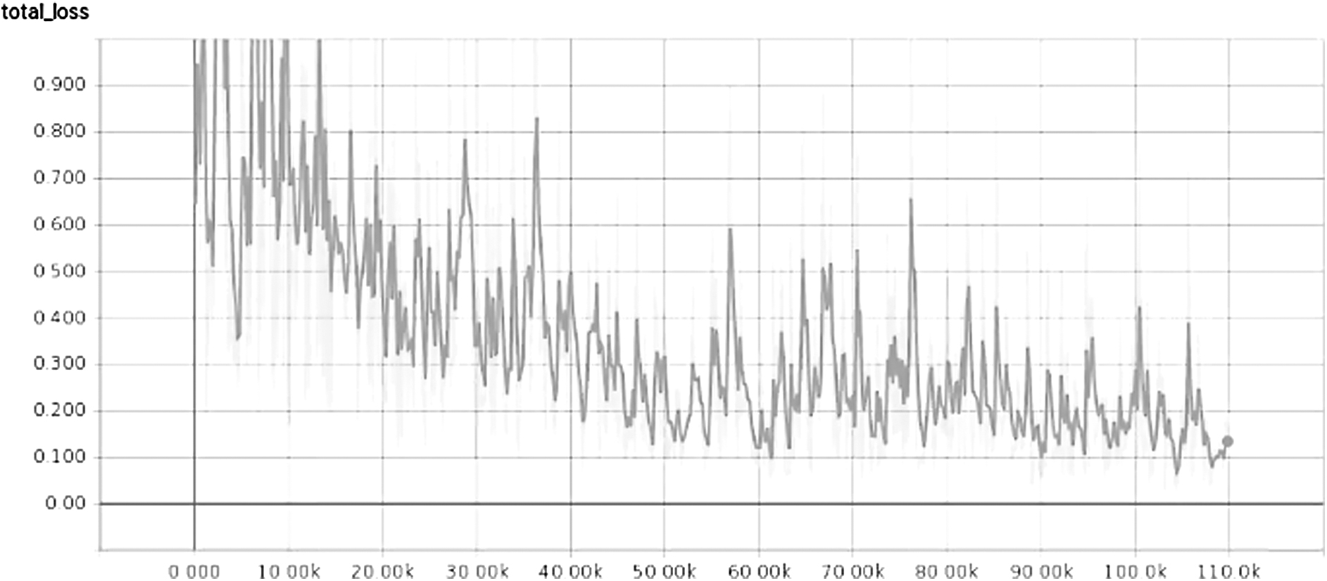
Loss function minimization using Pascal_voc 2007 and Pascal_voc 2012 for training.

Table 3.

Minimum of the loss functions

Training data	Pascal_voc 2007 + Pascal_voc 2012	COCO
Minimum of the classification loss function	0.0648	0.0437
Minimum of the detector loss function	0.0435	0.0235
Minimum of the total loss function	0.1350	0.1191

Testing

Statistical tests are the best to evaluate machine learning models. In particular, assessing a deep learning model on a given data set allows choosing the model with the best skills. The best model will estimate skills when making the prediction. The minimum error or maximum accuracy was used to evaluate classification and regression problems. For the combination of both classification and regression in the same model, the mean AP was applied to evaluate the model performance. In this work, the mean average accuracy was chosen as a statistical test to determine our performance and compare them with existing models. Also, the paired t-test was deployed to evaluate the robustness of our proposed method against benchmark approaches.

After the training process, the proposed approach was tested using Pascal_voc 2007 then tested with Pascal_voc 2012 testing data set. As shown in Table 4, when training on Pascal_voc 2007 + Pascal_voc 2012 and testing with Pascal_voc 2007, we achieve 75.14% as mean AP, and when testing with Pascal_voc 2012, we achieve 72.41% as mean AP. The results attended outperform all the proposed region-based methods in terms of speed and precision. Also, our method outperforms other detection methods in terms of precision, such as YOLO.²¹ In addition, YOLO struggle with detecting small objects in the image, unlike our method that can detect any object whatever its size.

Table 4.

Results using Pascal_voc 2007 + Pascal_voc 2012 for training and testing with Pascal_voc 2007 and then with Pascal_voc 2012

Test data		AP per category (%)
Test data		Pascal_voc 2007	Pascal_voc 2012
Categories Pascal_voc 2007 Pascal_voc 2012	Aeroplan	76.28	73.32
	Bicycle	79.20	77.20
	Bird	74.78	71.70
	Boat	65.55	63.58
	Bottle	62.70	60.75
	Bus	82.67	80.62
	Car	87.22	86.32
	Cat	86.27	83.67
	Chair	59.50	49.50
	Cow	80.78	78.34
	Dining table	71.19	69.16
	Dog	84.71	82.91
	Horse	85.47	83.17
	Motorbike	77.40	75.80
	Person	78.77	76.17
	Potted plant	47.41	45.11
	Sheep	76.48	74.78
	Sofa	71.88	68.88
	Train	79.41	76.48
	Tv monitor	75.10	73.14
Mean AP		75.41	72.47

AP, average precision.

When we train our model using COCO data set and we test using Pascal_voc 2007 and Pascal_voc 2012 testing data set, the mean AP is enhanced. As shown in Table 5, if testing with Pascal_voc 2007, we achieve 77.45% as mean AP, and if testing with Pascal_voc 2012, we achieve 74.04% as mean AP. We notice that the mean AP gets enhanced when using a larger training data set. So, the augmentation of the training data set leads to better performance and that shows the importance of big data for improving the performance of deep learning models.

Table 5.

Results using COCO data set for training and testing with Pascal_voc 2007 and then with Pascal_voc 2012

Test data		AP per category (%)
Test data		Pascal_voc 2007	Pascal_voc 2012
Categories Pascal_voc 2007 Pascal_voc 2012	Aeroplan	78.46	70.62
	Bicycle	83.25	84.44
	Bird	75.57	74.78
	Boat	65.45	63.18
	Bottle	77.56	76.24
	Bus	81.64	64.56
	Car	84.19	83.82
	Cat	83.43	84.62
	Chair	69.45	67.42
	Cow	82.73	80.54
	Dining table	75.66	74.28
	Dog	81.83	68.91
	Horse	84.19	81.27
	Motorbike	79.93	70.88
	Person	67.47	74.15
	Potted plant	83.57	58.64
	Sheep	78.28	72.87
	Sofa	79.55	73.38
	Train	82.84	79.43
	Tv monitor	79.47	71.64
Mean AP		75.41	77.45

Table 6 represents a comparison with other detection methods. Some of those methods are region proposal based,^10,12,17,27 and others such as YOLO.²¹ To fairly compare our method with the existing methods, we use the same data sets used by those works. In some cases, they do not use COCO data set. So, we use the Pascal voc data sets for training and testing to be able to compare our work with existing works. To test the model trained with COCO data set using Pascal voc data sets, the 20 classes provided by Pascal voc data sets were taken in account.

Table 6.

A comparison with other works in object detection

Structure	Training data	Mean AP (%)		Speed (FPS)
Structure	Training data	Pascal_voc 2007	Pascal_voc 2012	Speed (FPS)
R-CNN¹⁰	2007	66.0	—	0.05
R-CNN¹⁰	2007 + 2012	—	—	0.05
Fast R-CNN¹²	2007	66.9	65.7	0.2
Fast R-CNN¹²	2007 + 2012	70.0	68.4	0.2
Faster R-CNN ZF net¹⁷	2007	56.3	55.2	4
Faster R-CNN ZF net¹⁷	2007 + 2012	59.9	56.8	4
Faster R-CNN VGG net¹⁷	2007	69.9	67.0	3
Faster R-CNN VGG net¹⁷	2007 + 2012	73.2	70.4	3
Faster R-CNN RES net²⁷	2007	—	—	2
Faster R-CNN RES net²⁷	2007 + 2012	76.4	73.8	2
YOLO²¹	2007	—	—	45
YOLO²¹	2007 + 2012	63.4	57.9	45
YOLO v2³⁷	2007 + 2102	76.8	—	40
Ours	2007	70.13	68.54	16
	2007 + 2012	75.41	72.47
	COCO	77.45	74.79

Our method outperforms all the state-of-the-art models for object detection those who use region proposed method or other methods.

YOLO, you only look once.

Our data set was divided into two nonoverlapping sets: training and test set, we only train on the one set and test on the other. To demonstrate the significance of the improvements made by the proposed approach, we apply a paired t-test. We suppose that the null hypothesis is that the mean of the AP differences over all the data set categories is zero. So, we compare the difference between the two methods by the difference of the AP of each category of the data set. Table 7 summarizes the different obtained p-values by comparing our model against the faster R-CNN with VGG Net and the YOLO model. The p-value of our method against the faster R-CNN is less than 0.05, and the p-value of our model against the YOLO model is also less than 0.05. The obtained results prove that there is a significant difference against the benchmark models. The proposed model has a considerable improvement against the faster R-CNN model and the YOLO model.

Table 7.

p-Value of the paired t-test

	p-Value
Ours vs. faster R-CNN	0.04
Ours vs. YOLO	<0.001
Faster R-CNN vs. YOLO	<0.001

Our method outperforms the most state-of-the-art models in object detection challenges. Especially when we augment the training data set, our model achieves higher performance. In terms of speed, our model outperforms all-region proposal methods, but it is slower than other methods, such as YOLO. In effect, the speed can be enhanced using a better GPU. The proposed CNN model achieved a good speed precision trade-off.

Thus, we implement our model in an object detection application to test our proposed approach. The model can manipulate 16 images per second with a precision per object higher than 95% of confidence. Figure 7 represents a sample of the output images of our application. The proposed method works very well on static images and achieves high performance in both detection and identification tasks. The model can distinguish between human acting such as a road panel and the real road panel. Also, the model can detect objects whatever the size of the object. So, the model can detect objects that take all the size of the image or a small object in the middle of the image and it can identify it correctly.

FIG. 7.

Output of the proposed approach.

Conclusion

Deep learning is the key to the most artificial intelligent application. Deep learning is the best solution to manipulate big data and to solve their challenges because it is an artificial intelligence function that mimics the workings of the human brain in data processing and the creation of models for decision-making.

In this article, we choose to solve object detection and identification task. Thus, we proposed a CNN to deal with this challenge. The main contribution of this work is to build a CNN that provides a good trade-off between speed and accuracy. The achieved results outperform the state-of-the-art models. The proposed CNN impose some limitation in term of computation resources and storage, but the use of GPU solves the issue. Using a GPU with more performance can enhance the performance of the proposed CNN in terms of processing speed. As future work, the proposed CNN can be fine-tuned using bigger data sets to enhance the accuracy.

Footnotes

Author Disclosure Statement

No competing financial interests exist.

Funding Information

No funding was received.

Cite this article as: Ayachi R, Said Y, Atri M (2021) A convolutional neural network to perform object detection and identification in visual large-scale data. Big Data 9:1, 41–52, DOI: 10.1089/big.2019.0093.

Abbreviations Used

References

Pierpaoli

, Jezzard

, Basser

, et al. Diffusion tensor MR imaging of the human brain. Radiology. 1996; 201:637–648.

Lumer

, Friston

, Rees

. Neural correlates of perceptual rivalry in the human brain. Science. 1998; 280:1930–1934.

Hassaballah

, Awad

, eds. Deep learning in computer vision: Principles and applications. Boca Raton, FL: CRC Press, 2020.

Deng

, Liu

, eds. Deep learning in natural language processing. Cham, Switzerland: Springer, 2018.

LeCun

, Kavukcuoglu

, Farabet

Convolutional networks and applications in vision. In: Proceedings of 2010 IEEE International Symposium on Circuits and Systems. Paris, France: IEEE, 2010, pp. 253–256.

Uijlings

JRR

, Van De Sande

KEA

, Gevers

, et al. Selective search for object recognition. Int J Comput Vis. 2013; 104:154–171.

Carreira

, Sminchisescu

. CPMC: Automatic object segmentation using constrained parametric min-cuts. IEEE Trans Pattern Anal Mach Intell. 2011; 34:1312–1328.

Arbeláez

, Pont-Tuset

, Barron

, et al. Multiscale combinatorial grouping. In: IEEE Conference on Computer Vision and Pattern Recognition (CVPR). Columbus, OH: IEEE, 2014, pp. 328–335.

Alexe

, Deselaers

, Ferrari

. Measuring the objectness of image windows. IEEE Trans Pattern Anal Mach Intell. 2012; 34:2189–2202.

10.

Girshick

, Donahue

, Darrell

, et al. Rich feature hierarchies for accurate object detection and semantic segmentation. In: Proceedings of the IEEE Conference on Computer Vision and Pattern Recognition. Columbus, OH: IEEE, 2014, pp. 580–587.

11.

, Zhang

, Ren

, et al. Spatial pyramid pooling in deep convolutional networks for visual recognition. IEEE Trans Pattern Anal Mach Intell. 2015; 37:1904–1916.

12.

Girshick

Fast R-CNN. In: Proceedings of the IEEE International Conference on Computer Vision. Santiago, Chile: IEEE, 2015, pp. 1440–1448.

13.

Sermanet

, Eigen

, Zhang

, et al. Overfeat: Integrated recognition, localization and detection using convolutional networks. arXiv preprint arXiv: 1312.6229, 2013.

14.

Erhan

, Szegedy

, Toshev

, et al. Scalable object detection using deep neural networks. In: Proceedings of the IEEE Conference on Computer Vision and Pattern Recognition. Columbus, OH: IEEE, 2014, pp. 2147–2154.

15.

Pinheiro

, Collobert

, Dollár

Learning to segment object candidates. In: Cortes C (ed). Advances in neural information processing systems. Montréal, Canada: MIT Press, 2015, pp. 1990–1998.

16.

Ayachi

, Afif

, Said

, et al. Strided convolution instead of max pooling for memory efficiency of convolutional neural networks. In: International Conference on the Sciences of Electronics, Technologies of Information and Telecommunications, Cham: Springer, 2018. pp. 234–243.

17.

Ren

, He

, Girshick

, et al. Faster R-CNN: Towards real-time object detection with region proposal networks. In: Cortes C (ed). Advances in neural information processing systems. Montréal, Canada: MIT Press, 2015, pp. 91–99.

18.

Long

, Shelhamer

, Darrell

Fully convolutional networks for semantic segmentation. In: Proceedings of the IEEE Conference on Computer Vision and Pattern Recognition. Boston, MA: IEEE, 2015, pp. 3431–3440.

19.

Simonyan

, Zisserman

. Very deep convolutional networks for large-scale image recognition. arXiv preprint arXiv: 1409.1556, 2014.

20.

Zeiler

, Fergus

Visualizing and understanding convolutional networks. In: European Conference on Computer Vision, Cham: Springer, 2014. pp. 818–833.

21.

Redmon

, Divvala

, Girshick

, et al. You only look once: Unified, real-time object detection. In: Proceedings of the IEEE Conference on Computer Vision and Pattern Recognition. Las Vegas, NV: IEEE, 2016, pp. 779–788.

22.

Mishkin

, Sergievskiy

, Matas

. Systematic evaluation of convolution neural network advances on the imagenet. Comput Vis Image Underst. 2017; 161:11–19.

23.

Krizhevsky

, Sutskever

, Hinton

. Imagenet classification with deep convolutional neural networks. In: Bartlett P (ed). Advances in neural information processing systems. Lake Tahoe, NV: MIT Press, 2012, pp. 1097–1105.

24.

Deng

, Dong

, Socher

, et al. Imagenet: A large-scale hierarchical image database. In: 2009 IEEE Conference on Computer Vision and Pattern Recognition. Miami, FL: IEEE, 2009, pp. 248–255.

25.

The ImageNet Large Scale Visual Recognition Challenge (ILSVRC). Available online at http://www.imagenet.org/challenges/ILSVRC/ (last accessed September 16, 2020).

26.

Szegedy

, Liu

, Jia

, et al. Going deeper with convolutions. In: Proceedings of the IEEE Conference on Computer Vision and Pattern Recognition. Boston, MA: IEEE, 2015, pp. 1–9.

27.

, Zhang

, Ren

, et al. Deep residual learning for image recognition. In: Proceedings of the IEEE Conference on Computer Vision and Pattern Recognition. Las Vegas, NV: IEEE, 2016, pp. 770–778.

28.

Fukushima

Neocognitron: A self-organizing neural network model for a mechanism of pattern recognition unaffected by shift in position. Biol Cybern. 1980; 36:193–202.

29.

LeCun

, Bottou

, Bengio

, et al. Gradient-based learning applied to document recognition. Proc IEEE. 1998; 86:2278–2324.

30.

De Mauro

, Greco

, Grimaldi

. A formal definition of Big Data based on its essential features. Libr Rev. 2016; 65:122–135.

31.

Snijders

, Matzat

, Reips

U-D

. “Big Data”: big gaps of knowledge in the field of internet science. Int J Internet Sci. 2012; 7:1–5.

32.

Dedić

, Stanier

Towards differentiating business intelligence, big data, data analytics and knowledge discovery. In: International Conference on Enterprise Resource Planning Systems, Cham: Springer, 2016. pp. 114–122.

33.

Wang

The challenges and promises of Big Data—An engineering perspective. In: International Workshop of Advanced Manufacturing and Automation, Singapore: Springer, 2017. pp. 599–604.

34.

Hashem

IAT

, Yaqoob

, Anuar

, et al. The rise of “big data” on cloud computing: Review and open research issues. Inf Syst. 2015; 47:98–115.

35.

Everingham

, Eslami

SMA

, Van Gool

, et al. The pascal visual object classes challenge: A retrospective. Int J Comput Vis. 2015; 111:98–136.

36.

Lin

T-Y

, Maire

, Belongie

, et al. Microsoft coco: Common objects in context. In: European Conference on Computer Vision, Cham: Springer, 2014. pp. 740–755.

37.

Redmon

, Farhadi

YOLO9000: better, faster, stronger. In: Proceedings of the IEEE Conference on Computer Vision and Pattern Recognition. Honolulu, HI: IEEE, 2017, pp. 7263–7271.