Deep Learning on Big,Sparse,Behavioral Data

Abstract

The outstanding performance of deep learning (DL) for computer vision and natural language processing has fueled increased interest in applying these algorithms more broadly in both research and practice. This study investigates the application of DL techniques to classification of large sparse behavioral data—which has become ubiquitous in the age of big data collection. We report on an extensive search through DL architecture variants and compare the predictive performance of DL with that of carefully regularized logistic regression (LR), which previously (and repeatedly) has been found to be the most accurate machine learning technique generally for sparse behavioral data. At a high level, we demonstrate that by following recommendations from the literature, researchers and practitioners who are not DL experts can achieve world-class performance using DL. More specifically, we report several findings. As a main result, applying DL on 39 big sparse behavioral classification tasks demonstrates a significant performance improvement compared with LR. A follow-up result suggests that if one were to choose the best shallow technique (rather than just LR), there still would often be an improvement from using DL, but that in this case the magnitude of the improvement might not justify the high cost. Investigating when DL performs better, we find that worse performance is obtained for data sets with low signal-from-noise separability—in line with prior results comparing linear and nonlinear classifiers. Exploring why the deep architectures work well, we show that using the first-layer features learned by DL yields better generalization performance for a linear model than do unsupervised feature-reduction methods (e.g., singular-value decomposition). However, to do well enough to beat well-regularized LR with the original sparse representation, more layers from the deep distributed architecture are needed. With respect to interpreting how deep models come to their decisions, we demonstrate how the neurons on the lowest layer of the deep architecture capture nuances from the raw fine-grained features and allow intuitive interpretation. Looking forward, we propose the use of instance-level counterfactual explanations to gain insight into why deep models classify individual data instances the way they do.

Introduction

The past decade has seen an explosion of interest in deep learning (DL) techniques. Experimental research has demonstrated significant improvements over conventional machine learning techniques in fields such as object recognition^1–3 and natural language processing.^4,5 DL techniques automatically create efficient distributed representations.⁶ By stacking nonlinear functions, hidden and complex data patterns can be learned with substantially less human feature engineering. The increased success of DL can be attributed to (1) an immense increase in available data, (2) increased chip processing capabilities and the use of graphics processing units (GPUs) for faster parallel computations, (3) declining costs of hardware, and (4) advances in machine learning research on DL, such as the introduction of new methods for avoiding overfitting.^7,8

Since the initial successes of DL, it has also been successfully applied to high-dimensional data such as toxicological data,^9,10 biomedical data,¹¹ and recommender systems.^12,13 This raises the question whether the superior performance of DL also extends to other types of data and applications,¹⁴ especially to data where nonlinear models have not excelled in prior research. Specifically, this study assesses the use of DL for classification with big sparse behavioral data. The application to such data is promising, due to their high dimensionality and the intuitively likely presence of important latent structure.

As people act in our digitally instrumented world, computer systems often record the trails we leave behind. These form behavioral big data. Let us define behavioral big data following Shmueli¹⁵: “very large and rich high-dimensional data on human actions and/or interactions.” Customer transactions with a bank, web surfers' webpage visiting behavior, mobile phone users' visited locations, and Facebook “likes” are just a few examples where each unique merchant, webpage, location, or liked page can correspond to a raw feature. Such data provide significant potential to support predictive analysis.¹⁶ In prior research, such data have been shown to be remarkably predictive and can reveal a person's personality traits,¹⁷ interest in banking products,¹⁸ interest in a news article,¹⁹ interest in a mobile ad,²⁰ credit default risk,²¹ tendency to churn,²² or tendency to commit fraudulent activities.²³

What is different from traditional classification settings is that such ultrahigh-dimensional behavioral data also are ultrasparse.²⁴ When modeling a web surfer's web visiting behavior, the collection of all possible webpages one can visit is huge. However, humans face a limit on their “behavioral capital”²⁴; for example, among all possible webpages, a person can only visit a limited number due to resource restrictions (mainly time in our example); among all possible merchants, a person can only transact with a limited number. The resultant behavioral data, therefore, are extremely sparse.

Predictive modeling from behavioral data is complicated by the fact that the processes generating the data are not well understood and often do not align with the assumptions on which our traditional modeling techniques are based.^15,25 Traditionally, machine learning research for very high-dimensional data mostly employs shallow models,⁷ which contain one layer for transforming the raw input features, in a linear or nonlinear manner, into a specific feature space. Examples of such techniques are linear or kernalized support vector machines.²⁶

When confronted with data from complex real-world processes such as human behavior, many researchers have questioned whether shallow techniques will suffice.^7,27 In particular, behavioral data are suspected (by social scientists as well as machine learning researchers) to contain complex, distributed, and hierarchical relationships between its features.^28,29 A distributed representation transforms the raw features through many-to-many relations into a new representation, which is able to capture fine-grained similarities between the independent features. At the lowest level, a user can be represented by each movie he or she has watched. On a higher level, a subset of movies can be telling of the person's (latent) interests. One group of movies can, for example, represent whether a user has an affinity with LGBT topics, whether he has an interest in sports, or whether he favors director Alfred Hitchcock. On an even higher level, these interests can reveal political preferences or religious beliefs. For example, a person watching movies such as Brokeback Mountain or Cowspiracy can be estimated to have a more liberal mindset. This line of thinking follows the value–attitude–behavior model²⁹ used in behavioral science, which states that people's social cognitions resulting in actions are organized in a compositional structure. Values are one's stable beliefs on the highest level of abstraction and are constructed of basic beliefs, which, in turn, give rise to value orientations. The latter influences a person's attitude, which finally leads to concrete human behavior.

The main drawbacks of DL methods, in contrast, are three. (1) The lack of solid theory as to why they work so well makes applying them highly dependent on the skill of the engineers and/or massive trial and error.⁷ (2) The inner workings of a complex learned deep network are generally considered to be difficult to understand (at best).^30–32 (3) Learning accurate deep networks from large data can be extremely time and resource consuming.^32,33

In previous research specifically focusing on high-dimensional behavioral data, DL has been applied to movie preference data¹² and e-commerce activity data³⁴ (although in these cases through applying dimensionality reduction techniques). In this article, we build deep predictive models using the complete behavioral feature space and we allow the opportunity for the models to exploit all the information inherent to the data.

This study contributes to the literature in four ways: (1) first, this study presents a careful report on a systematic application of DL to big behavioral data; (2) second, we analyze the performance of DL techniques and compare it with the performance of well-regularized logistic regression (LR) (previously shown to excel on this sort of data) to assess whether and when DL can provide significant performance improvements; (3) third, we provide guidance for researchers and practitioners regarding the practical implementation details that work well (or not) for such data; and (4) finally, we attempt to give a high-level preliminary insight into why deep models work well on behavioral data and how they can be interpreted.

In what follows, first we give a brief overview of DL. We discuss in detail the specific architectural and training choices used for the experiments, paying particular attention to hyperparameter (HP) selection. We present the behavioral data used to evaluate and compare. We then present and discuss the result of comparing the predictive performance with the reigning best machine learning method for data such as these, as revealed by multiple prior studies.

DL Overview

When using DL for classification,^7,14,35 we have a data set D, an indexed set of n data points $x_{i}$ with n corresponding labels y_i, with $x_{i} \in ℛ^{m}$ and $y_{i} \in - 1, 1$ for $i = 1, \dots, n$ . A classifier learning algorithm A takes a subset of the data set D, called a training set $D_{t r a i n} = (X_{t r a i n}, Y_{t r a i n})$ as input and learns a hypothesis function (model) f as an approximation of the true data distribution: $f = A_{λ} (X_{t r a i n}, Y_{t r a i n}),$ (1)

with modeling HPs $λ$ . In the specific context of DL, the number of layers L is an example of a HP. Good settings for the HPs $λ$ are learned via a separate subset of D referred to as a validation set $D_{v a l} = (X_{v a l}, Y_{v a l})$ . The learning algorithm chooses a model f by (approximately) minimizing a loss function $ℒ$ over a set of model parameters $θ$ $m i n_{θ} ℒ (f (X_{t r a i n}), Y_{t r a i n}) .$ (2)

The final classification performance of the learned model is tested on a separate test set $D_{t e s t} = (X_{t e s t}, Y_{t e s t})$ .

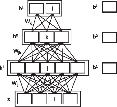
The DL algorithm is applied to a particular network architecture (of which a concrete example is shown in Fig. 1) and minimizes the loss function $ℒ$ over its parameters $θ$ (consisting of weight parameters W and bias parameters $b$ ) through backpropagation by stochastic gradient descent (SGD).³⁶,* The backpropagation training algorithm works in two stages: (1) (forward) propagation and (2) parameter update. In the forward pass, starting with (randomly chosen small) initial values for the weights W and the biases $b$ , a batch of training samples is taken as input. The learner computes the corresponding activations and the output values and compares them to the real labels.

FIG. 1.

Example of a deep learning network with two hidden layers $h^{1}$ and $h^{2}$ and their associated bias vectors $b$ and weight matrices W.

Next, the gradient of the error is used in a backward pass to update the model's parameters W and $b$ for each layer at iteration t $W^{h} (t + 1) = W^{h} (t) + α \frac{\partial ℒ}{\partial W^{h}} + ξ (t),$ (3)

b^{h} (t + 1) = b^{h} (t) + α \frac{\partial ℒ}{\partial b^{h}} + ξ (t),

(4)

where $α$ is a learning rate and $ξ$ an error component. Using SGD requires that the loss function $ℒ$ be differentiable. Negative log likelihood minimizes the negative likelihood of the correct class and is differentiable: $N L L = - \sum_{i = 0}^{n} l o g P (Y = y_{i} | x_{i}, θ) .$ (5)

The objective function (2) of the DL problem formulation does pose difficulties. It defines a nonconvex optimization space characterized by multiple local optima, contributing to an inherently complex learning process. Using a local optimization technique such as SGD may result in the model getting stuck at local optima and thus may result in poor generalization performance.²⁷ Moreover, with a large number of layers and many hidden units, the number of model parameters can be massive, which requires a large amount of data to properly control complexity and not overfit.^†^,37

A second difficulty faced by DL algorithms is that the algorithms and the models they produce are often condemned to being black boxes, due to the many layers, many learned parameters, and the models' cascading nonlinearities.

DL architecture and training

For this study, we apply DL following the best practices recommended by existing articles, practical guides, and textbooks (as well as we can).^‡ DL architectures are characterized by a large number of HPs.^35,36 The values of the HPs associated with a machine learning model f are selected based on their (joint) performance on the separate out-of-sample validation set $(X_{v a l}, Y_{v a l})$ . Two types of HPs can be distinguished: (1) HPs associated with the model, such as the number of hidden units per layer, and (2) HPs associated with the optimization algorithm such as the learning rate of SGD. The HP optimization problem can be modeled as follows: $λ_{o p t} = {argmin}_{λ_{h p}} ℒ (f (X_{v a l}), Y_{v a l}),$ (6)

where $λ_{o p t}$ is the optimal HP set that is found by searching over the validation data.³⁵ Each $λ_{h p}$ is a collection of values for each of the K HPs: $(H P_{1}, \dots, H P_{K})$ .

To select appropriate values for the HPs in an empirical setting, a structured method is needed to search the HP space.³⁵ When DL models are trained in the literature, HPs often are chosen either based on researchers' experience in the specific field or through a structured or heuristic exploration of the HP space, such as manual search, grid search, or random search.³⁵ We are training deep neural networks on a sort of data where there is little specific experience to rely on for selecting HP values. (Reporting on such an experience for this sort of data is one contribution of this article.) Moreover, although they share similar characteristics, this study applies DL to many different data sets, for which separately optimized HPs should be used.³⁵

Bergstra and Bengio³⁵ observe that from the large collection of all HPs, usually only a small subset is relevant (referred to as low effective dimensionality). Their study empirically and theoretically demonstrates that nonadaptive random HP search is more efficient than manual search and/or grid search in high-dimensional search spaces. Although a high-dimensional grid may give even coverage over the grid, the coverage in the separate subspaces is less-evenly distributed. In contrast, random search counterintuitively explores a wider range in each of the subspaces. Therefore, we use random HP search³⁵ to evaluate 100 parameter configurations on the validation data $(X_{v a l}, Y_{v a l})$ . These configurations are optimized for negative log likelihood; their validation area under the ROC curve (AUC) is calculated, and the best configuration is chosen.³⁹ The specific values and possible ranges for each HP are given in the next subsections.

After selecting the best HP configuration, five-fold cross-validation³⁷ is used on the remaining data. During learning, progress is monitored by calculating the negative log likelihood on a separate part of the training set, which is used to prevent overfitting by early stopping.⁴⁰ Finally, the AUC is calculated on a separate test set after the learning is complete. We repeat this procedure for each of the five folds, resulting in five different AUC estimates measured on the test set. In other words, each iteration of cross-validation produces one estimate of generalization performance; thus, the AUC reported in our study is the average AUC on the test set measured over the five folds.

We ran the random HP search procedure and the actual learning algorithm on Amazon Web Services (AWS) g2.2xlarge instances with the Theano framework for DL.⁴¹ These instances have 8 virtual CPUs, 15 GB RAM, and 1 Nvidia grid GPU.

Unsupervised pretraining

Unsupervised pretraining was one of the main reasons for the increased attention toward DL starting in 2006, due to significant classification performance improvements.⁴² This pretraining phase uses a stack of representation learning algorithms (such as restricted Boltzmann machines [RBMs]³⁶) and separately optimizes the learned representation of each layer in an unsupervised manner. The goal is to use the learned representation of the unsupervised stage for a classification task with the same input data distribution. The idea behind greedy layer-wise pretraining originates from the following two beliefs: (1) the initial parameters can have an effect on the quality of the parameter optimization process and subsequently influence model performance during model fine tuning, and (2) the representation learned by a generative model on unlabeled input data can also be a good representation for a subsequent classification task.²⁷

Previous research has demonstrated the immense value in pretraining a neural network.^40,42 Erhan et al.⁴⁰ empirically analyze the effect of pretraining and conclude that it mainly acts as a regularizer, influencing the starting point of the supervised training step. However, the study by Erhan et al.⁴⁰ was performed before the widespread use of many modern DL-related concepts such as rectified linear units (ReLUs)⁴³ and only takes into account the relationship with the number of layers.

We let the use of pretraining be a HP. In the random HP search, we choose to either pretrain the network or not through the use of a RBM.³⁶

Number of layers and number of hidden units

Both the number of hidden layers and the number of units they incorporate have an impact on the generalization capacity of the network. The HP search attempts to manage the critical trade-off between generalization ability on the one hand and overfitting on the other. For each HP combination, a number of hidden layers between 1 and 8 is selected; for each layer, a number of hidden units is drawn log-uniformly between 18 and 2000. Both ranges are based on HP values used by Bergstra and Bengio.³⁵

Minibatch size

Most modern optimization algorithms for DL do not use the entire training set at once, instead choosing more than one but fewer than all training examples at a time,³⁸ which is referred to as a minibatch. Choosing the size of the minibatch for SGD is a two-criteria trade-off influencing convergence and training time. When increasing the size of the batch, more efficient use can be made of the parallel matrix–matrix multiplications on the GPU.³⁶ Although the stochastic gradient estimates become more reliable with larger minibatch sizes, using fewer batches reduces the number of weight updates, thereby reducing optimization convergence.³⁶

In contrast, closely approximating the true gradient by increasing the size of the minibatch might not be the best choice to spend computation time in a nonconvex optimization space. Instead, exploring the search space with frequent updates may be a more appropriate tack, as a smaller minibatch size has been shown to increase generalization performance.⁴⁴ Furthermore, a small minibatch size acts as a regularizer, introducing noise when approximating the gradient through a smaller number of training set instances.³⁶

Following the literature,^35,36 our HP search chooses the size of the minibatch randomly with equal probability between 20 and 100. In each epoch, each fold is randomly shuffled before minibatches are selected to speed up convergence.³⁶

Nonlinear activation function

The activation function of a neural network brings nonlinearity into the learning procedure. When choosing an activation function, care must be taken regarding the saturation of the activations and overly linear behavior.¹⁴ If activations in the network become too saturated during learning, the gradients do not propagate well and units become inactive. If the functions behave in a linear manner, complex interactions will not be learned.¹⁴ We consider the three most commonly used nonlinearities: the sigmoid, the hyperbolic tangent, and the ReLU. The HP selection randomly chooses one. These nonlinear activation units are elaborated in detail in Appendix A1.

Learning rate

The learning rate of the SGD optimization algorithm can influence convergence toward an optimum. If the learning rate is set too high, optima can be overlooked and the loss function will increase. In contrast, too small a learning rate results in very slow convergence.

Our random HP search algorithm draws an initial learning rate $α_{0}$ log-uniformly between 0.0000001 and 1.0 with an adaptive annealing scheme. If at iteration t, the previous solution is not found to be better than the current solution in the optimization algorithm (given a specific improvement threshold), $α_{t}$ is set as follows: $α_{t} = \frac{t \cdot α_{t - 1}}{m a x (t, t + 1)}$ .³⁵

Data

To evaluate the predictive performance of DL on large-scale behavioral data, we use behavioral data sets from prior research. We start with the collection presented by De Cnudde et al.⁴⁵ to benchmark machine learning methods on this sort of data. (De Cnudde et al.⁴⁵ did not compare with DL.) To this collection we add a collection of data sets predicting personal traits based on the things people “like” on Facebook.^17,25,46,47

The MovieLens and YahooMovies data sets, for which we predict the ages and the genders of the users, contain data regarding which movies are rated by which users. The task for the larger MovieLens10m data set is to predict the genre of a movie based on the users rating it. This multiclass classification task is translated into 18 binary classification problems. The Ecommerce data set provides product viewing data on an e-commerce website from which the genders of the users are to be inferred. Shopping transactions in the TaFeng data set are used to predict users' ages. In the BookCrossing data set, books are rated by the members of the BookCrossing community, and based on these ratings, the ages of the users are predicted. The LibimSeTi data set contains ratings of dating profiles from which the genders of the users are to be inferred. In 2015, the KDD Cup challenge KDD2015 constituted the prediction of massive open online courses dropout based on fine-grained course interaction data. The Fraud data set contains financial transactions between companies to determine whether a company is involved in corporate residence fraud.²³ A consumer's interest in an online car advertisement is to be predicted based on his or her website viewing behavior in the Car data set. In the Flickr data set, users have tagged pictures as their favorites, from which a picture's number of comments is to be predicted. Lastly, the Facebook data sets include users “likes” of pages on Facebook from which the following target variables are to be predicted: intelligence, religion (Christian vs. Muslim), satisfaction with life, political belief (liberal vs. conservative), gay for male and female users, and gender. Table 1 lists the main characteristics of these data sets, and as one can observe, the dimensionality and the sparsity (measured as one minus the percentage of matrix entities that are “active,” which means that they are not zero) both are extremely high. The number of active elements reports the actual number of nonzero matrix entries.

Table 1.

Behavioral data sets

Data set	Target variable	No. of targets	Instances	Features	Active elements	Sparsity, %
MovieLens100k	Age/gender	2	943	1682	100,000	93.6953
MovieLens1m	Age/gender	2	6040	3883	1,000,209	95.7353
KDD2015	MOOC dropout	1	120,542	5891	1,919,150	99.7300
Ecommerce	Gender	1	15,000	21,880	33,455	99.9898
TaFeng	Age	1	31,640	23,719	723,449	99.9036
MovieLens10m	Genre	1	10,681	69,878	10,000,053	98.6602
YahooMovies	Age/gender	2	7642	106,363	221,330	99.9727
Fraud	Fraudulent	1	858,131	107,345	1,955,912	99.9979
Facebook	IQ	1	6124	128,787	850,181	99.8922
Facebook	Religion	1	4913	128,787	388,973	99.9385
Facebook	Satisfaction with life	1	30,138	128,787	2,873,825	99.9260
Facebook	Political belief	1	38,099	128,787	2,214,178	99.9549
Facebook	Gay (male)	1	172,191	128,787	11,171,527	99.9496
Facebook	Gay (female)	1	214,130	128,787	16,546,926	99.9400
Facebook	Gender	1	386,321	128,787	27,718,453	99.9443
LibimSeTi	Gender	1	137,806	220,970	15,656,500	99.9486
BookCrossing	Age	1	167,175	337,921	838,364	99.9985
Flickr	Comments	1	11,195,144	497,472	34,645,469	99.9994
Car	Interest in ad	1	9,108,905	2,936,810	65,464,708	99.9998

The target variables are all binary. The table is sorted by number of features.

MOOC, massive open online courses.

What to Compare Against?

De Cnudde et al.⁴⁵ present a comparative study of 11 widely used classification techniques applied to high-dimensional sparse behavioral data sets. They compare variations of support vector machines, naive Bayes, LR, and a relational classifier called pseudosocial network (PSN). For details regarding the techniques and their parameters, and the results, please see their article.⁴⁵ Their results show that LR with L2-regularization and batch gradient descent (LR-BGD-L2) produces overall the best results (significantly) in terms of AUC, as compared with the other shallow learners. Therefore, for our main results we compare DL with LR-BGD-L2. Note that despite LR-BGD-L2 being the best performer overall, for some specific data sets, other shallow learners such as PSN performed better than LR-BGD-L2. Thus, for completeness, Appendix A2 in Appendix A2 presents a comparison of DL with all the shallow classifiers compared in the article.⁴⁵ Please note that this prior benchmarking result is corroborated elsewhere; for example, the studies by Clark and Provost⁴⁷ and Chen et al.⁴⁶ also concluded (in different contexts) that compared with other non-DL methods, L2-regularized LR performed best on this sort of data.

Results and Discussion

To assess the performance of DL on behavioral data, we perform three analyses. First, we compare DL with LR-BGD-L2. The goal is to examine whether and (if so) when deep techniques are preferable for big behavioral data. Second, we dig deeper and analyze the influence of HP values on the classification performance for DL networks. Here, the goal is to get insight into the influence of choices of learning network architecture, characteristics of the optimization process, and unsupervised preprocessing. Third, we provide a preliminary view into why DL techniques perform well on behavioral big data and how they can be interpreted. To this end, we focus on the representation learning to try to understand the representations learned from these big behavioral data sets. The results and interpretations of these analyses are presented in each of the next subsections.

Performance of deep versus shallow learning

Table 2 gives the HP configuration for which the “best” results with DL are reached for each data set. (For all data sets, the best parameters come from nonpretrained models, hence, we have not included these HP results as an extra column.) Note that these configurations are not necessarily the best possible configuration for that data set. The configuration shown is the best performing configuration based on the selection procedure described previously. Different selection procedures or more computation could potentially lead to better classification performance. However, the computation time is already very high (2–3 days)—in both an absolute sense and relative to the competing LR—and the results (presented next) are unequivocal.

Table 2.

Best hyperparameter configuration for each data set from the random hyperparameter search procedure for the deep learning classification techniques

Data set	Number of layers and hidden units per layer	Nonlinearity	Learning rate α₀
BookCrossing	18, 72, 233, 175, 37	ReLU	0.43858
Facebook_swl	654, 90	ReLU	0.16641
TaFeng	194	tanh	0.04343
YahooMovies_age	736, 1392	ReLU	0.84896
Fraud	125, 212, 178	tanh	0.14347
Car	22, 43	ReLU	0.67745
MovieLens_adventure	47	ReLU	0.89871
MovieLens_100k_gender	545, 52, 166, 184	tanh	0.31278
Ecommerce	687, 45, 109, 31	tanh	0.24682
MovieLens_crime	1678, 363, 163, 95	tanh	0.01436
Facebook_female_gay	67, 243	sigmoid	0.52290
MovieLens_fantasy	63, 24, 324, 45, 1895	ReLU	0.18981
MovieLens_mystery	21	ReLU	0.61191
YahooMovies_gender	72, 995, 832, 1939	ReLU	0.02167
MovieLens_romance	95, 47, 794	ReLU	0.99152
MovieLens_thriller	93	ReLU	0.75717
MovieLens_drama	287, 1764, 32, 65	tanh	0.59338
KDD2015	130, 30, 99, 1388, 1533	sigmoid	0.44715
MovieLens_children	213, 69, 21, 182, 1130	tanh	0.88797
MovieLens_1m_gender	532, 135, 1009	ReLU	0.30452
MovieLens_comedy	19, 398	tanh	0.00540
Flickr	21, 25	ReLU	0.54377
MovieLens_action	45	tanh	0.94335
MovieLens_animation	288, 677, 772	ReLU	0.52020
MovieLens_scifi	23	sigmoid	0.56118
MovieLens_100k_age	48, 709	ReLU	0.11159
MovieLens_documentary	521, 78	sigmoid	0.20603
MovieLens_western	1345, 218, 1013	ReLU	0.86652
MovieLens_1m_age	1863, 93	tanh	0.14166
Facebook_religion	1414, 464, 71, 424, 60	tanh	0.09468
MovieLens_horror	171, 467	tanh	0.06355
Facebook_male_gay	473, 293	sigmoid	0.10999
MovieLens_filmnoir	1242	tanh	0.60603
Facebook_political	27, 146	tanh	0.76728
Facebook_IQ	129, 32	sigmoid	0.52109
MovieLens_musical	67, 656, 20, 1204	ReLU	0.75767
Facebook_gender	76, 367	ReLU	0.10510
MovieLens_war	248, 35, 694, 855	tanh	0.52687
LibimSeTi	96, 348, 36, 800, 47	sigmoid	0.01922

ReLU, rectified linear unit.

Table 3 gives the performance of the models learned with LR-BGD-L2 compared with the performance of those learned with DL. For each data set, the best classifier is denoted in boldface. At the bottom, the table also gives the average rank of the techniques (with the best-performing technique receiving rank 1) and the number of times it performs best. It is clear that, overall, DL is learning at least as well as or better than L2-regularized LR. DL has a lower average ranking (1.12 in contrast to 1.88) and it achieves a much higher number of wins (34 times in contrast to 4 times).

Table 3.

Predictive performance of the models in terms of area under the ROC curve for binary behavioral data sets

	DL	LR-BGD-L2
BookCrossing	55.32	56.25
Facebook_swl	55.67	56.23
YahooMovies_age	65.66	64.84
TaFeng	71.35	71.36
Fraud	77.22	55.48
Car	78.16	77.70
MovieLens_adventure	78.61	73.98
MovieLens_100k_gender	79.30	77.21
Ecommerce	76.34	79.62
MovieLens_crime	79.86	76.13
Facebook_female_gay	77.98	75.21
MovieLens_fantasy	80.83	62.22
MovieLens_mystery	80.65	68.03
YahooMovies_gender	81.35	80.43
MovieLens_romance	81.75	68.20
MovieLens_thriller	84.21	75.08
MovieLens_drama	84.72	83.74
KDD2015	85.26	79.89
MovieLens_children	85.46	79.7
MovieLens_1m_gender	85.63	85.20
MovieLens_comedy	87.04	86.13
Flickr	87.45	76.97
MovieLens_action	87.79	86.89
MovieLens_animation	88.31	87.10
MovieLens_scifi	89.08	79.66
MovieLens_100k_age	89.50	87.95
MovieLens_documentary	90.04	88.57
MovieLens_western	90.72	85.82
MovieLens_1m_age	91.39	90.81
Facebook_religion	92.02	86.91
MovieLens_horror	92.42	91.27
Facebook_male_gay	91.78	88.89
MovieLens_filmnoir	90.12	78.60
Facebook_political	93.63	84.10
Facebook_IQ	94.40	63.23
MovieLens_musical	95.02	80.53
Facebook_gender	93.47	87.89
MovieLens_war	95.45	80.74
LibimSeTi	99.69	99.69
Average ranking (AUC)	1.12	1.88
No. of wins (AUC)	34	4

The highest achieved performance for a data set is indicated in boldface. The table is sorted by maximum AUC.

AUC, area under the curve; DL, deep learning; LR-BGD-L2, logistic regression with batch gradient descent and L2-regularization.

However, we can observe the hint of an interesting phenomenon, which may deserve further research. Specifically, for the three data sets with the lowest signal-from-noise separability (defined next), data sets BookCrossing to TaFeng given in Table 3, DL consistently results in lower classification performance. We say “a hint” because drawing a solid conclusion from three data sets is dubious; however, these results do concur with the results from prior research. Perlich et al.⁴⁸ show that the suitability of linear (in particular, LR) versus nonlinear learning methods depends on the signal-from-noise separability of the data set. In particular, Perlich et al.⁴⁸ propose that the maximum AUC (max-AUC) achieved by any classification method is a good proxy for the ability of machine learning to produce models that separate signal from noise in a data set.

Figure 2 plots the difference between the AUC of DL and LR-BGD-L2 against the maximum AUC achieved by either DL or LR-BGD-L2. Points above the horizontal line (where y = 0) are data sets for which DL performs better. The graph clearly shows two regimes: first, when the max-AUC is high (0.8 and above), DL performs much better than LR for many data sets, and second, there is no data set for which DL performs worse than LR. When the max-AUC is <0.75, DL does not outperform LR. Curiously, the study by Perlich et al.⁴⁸ also showed a regime change at max-AUC = 0.8. Again, we do not have enough data sets in the lower separability regime to draw any clear conclusion; however, many popular DL successes are on data where the inherent signal-from-noise (SNS) separability is high. (Besides using max-AUC as a proxy, we can ask: how well can a human do the task?)

FIG. 2.

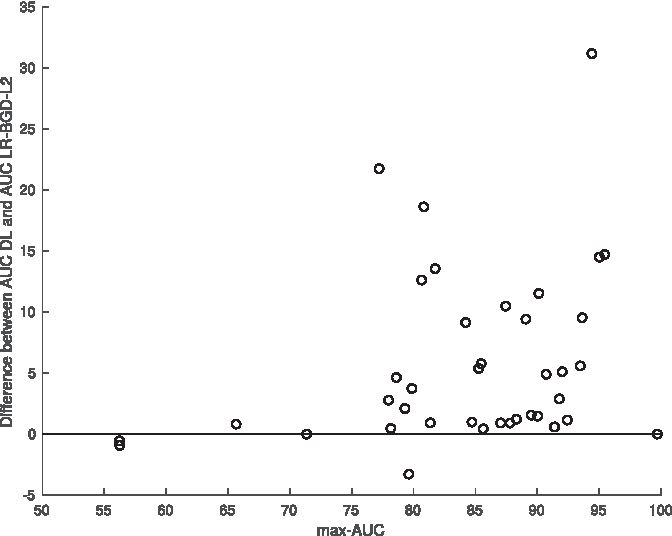
Difference between AUC of LR-BGD-L2 and DL plotted against max-AUC. Dots above the horizontal line denote data sets where DL outperforms LR-BGD-L2. AUCs are represented as percentages. AUC, area under the curve; DL, deep learning; LR-BGD-L2, logistic regression with batch gradient descent and L2-regularization.

We use the Wilcoxon signed-rank test to make a formal statistical comparison between the performance of DL and LR-BGD-L2.⁴⁹ For extrapolating the findings of this test to a larger population of behavioral data sets, ideally the data sets should form a random and representative sample of the population of all possible behavioral data sets. However, our data collection consists of multiple multitarget problems (Facebook, YahooMovies, and MovieLens), which are subsets of prediction problems with the same input vectors but different target variables. This may result in consistency regarding the performance of their classifiers. We take two different approaches, both used by De Cnudde et al.,⁴⁵ to address this. The first approach selects a random data set from each multitarget problem to represent the others. For example, of all seven classification problems using the Facebook data, only a randomly chosen problem is used for the statistical comparison (e.g., Facebook_political). The second approach assigns equal partial weights to the multitarget data sets in order for all information to be present in the analysis. For example, each of the seven classification tasks that makes the use of the Facebook “Like” data will only weigh a small bit in the total comparison. More specifically, the weight can be divided equally over the classification tasks that use Facebook data, such that each task gets a weight of 1/7th in the comparison. From Table 4 we conclude that both approaches lead to the same statistical conclusions, and for this reason, we only discuss the latter. Concretely, the test is performed with a sample size of 13 data sets.

Table 4.

Pairwise comparison between deep learning and L2-regularized logistic regression using (1) a random, representative sample or (2) a weighted approach for multiple multitarget problems

High SNS data only	Random sample	Weights	Sample size	p	Significant (α = 0.05)
X	X		13	0.0261	Yes
X	X		8	0.0078	Yes
		X	13	0.0212	Yes
		X	8	0.0078	Yes

SNS, signal-to-noise.

We find a p-value of 0.0212, which shows that DL performs marginally statistically significantly better than LR-BGD-L2. However, the performance improvement does not reach a 1% significance level. This can be attributed to (1) the additional complexity of DL merely resulting in marginal performance improvements on some data,⁵⁰ which thus do not contribute to statistical power, and (2) DL performing worse for low-SNS data, as discussed earlier.

To formalize the latter, we repeat the test using only the data sets that exceed the signal-from-noise separability threshold of 80% given in Perlich et al.⁴⁸ and we find a p-value of 0.0078. This shows that for high-SNS data sets, DL performs significantly better at a 1% significance level. Compared with the previous test results, the p-value is smaller (0.0078 in contrast to 0.0212); thus, we conclude that the signal-from-noise separability of the data set should be considered when deciding whether to invest significant resources in applying DL to big behavioral data.^§

The focus of the experiments was to compare the predictive performance of DL with the method that has been reported repeatedly to be the best method for high-dimensional sparse behavioral data—appropriately regularized well-optimized LR. Besides the scientific interest, such a comparison has practical import, for example, to give guidance into whether applying DL often may be worth the cost, since DL requires much more computational (and engineering) effort than LR. The results given show that for high-signal-from-noise-separability data sets, DL indeed generally yields better generalization performance (in terms of AUC). However, prior research also showed that LR is simply the overall best “shallow” method, not universally the best; other computationally efficient modeling techniques sometimes perform much better. Figure 3 shows the difference in performance between DL and the best shallow method reported for each data set by De Cnudde et al.⁴⁵ (all of those being relatively efficient computationally). We see that by this comparison, DL excels on fewer data sets (compared with Fig. 2), generally performing marginally better or on par with the best shallow method. Nevertheless, in terms of the number of wins, DL still outperforms the best shallow learner (27 in contrast to 11, see Appendix A2). The maximum difference in AUC between DL and the best shallow learner shown in Figure 2 is achieved when predicting intelligence quotient from the Facebook data, which indicates that DL is learning something nonlinear that is important for this task. This comparison has a serious limitation however: we cherry-picked the best method, which potentially suffers from overestimation of generalization performance due to statistical multiple comparisons. An interesting follow-up would be to conduct a careful study, choosing the best shallow method for each data set by cross-validation (the choice of shallow technique then becomes a HP). That way the generalization performances could be compared on equal footing, as well as the computational efforts required (note that running a whole bunch of shallow methods, and choosing the best using cross-validation, is not necessarily so computationally efficient, even if the individual techniques are).

FIG. 3.

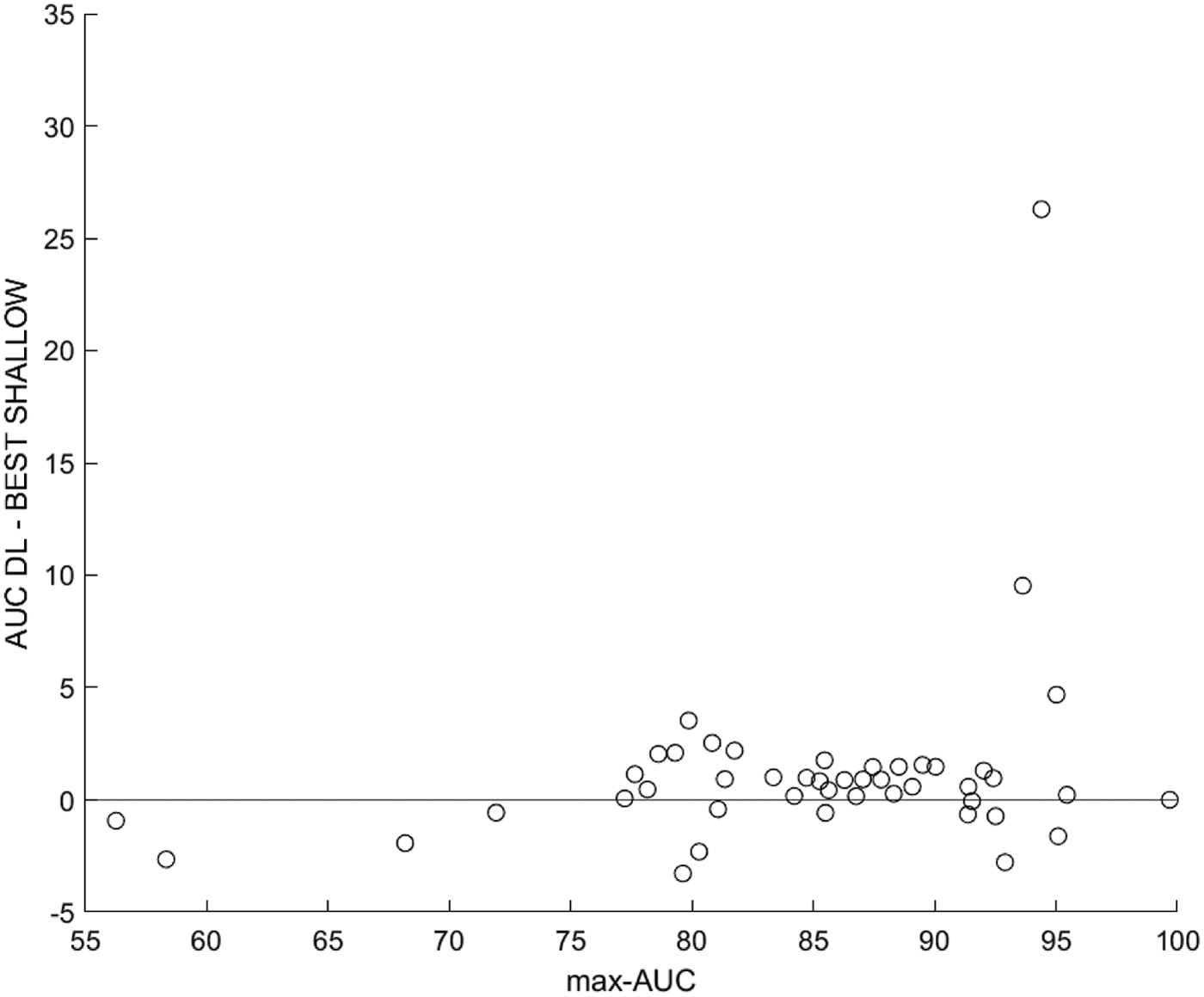
Difference between AUC of the best shallow model (chosen from 11 shallow classifiers) and DL plotted against max-AUC. Dots above the horizontal line denote data sets where DL outperforms the best shallow model.

Influence of HPs

When training the DL models and evaluating their generalization capacity, no improvement is found when using pretraining. Figure 4 shows the test classification error on the MovieLens1m data set for 500 different random configurations for which only the pretraining flag was changed. (Note that this figure is representative of the remaining data sets). It is clear from this comparison that not pretraining the network results in marginally lower test classification error on average, and more strikingly, substantially lower variance. Furthermore, pretraining the network substantially increases the training time, which already is very high for these data.

FIG. 4.

Test classification error for the MovieLens1m data set for predicting gender without pretraining (left) and with pretraining (right).

The fact that unsupervised pretraining does not improve classification performance is in line with prior non-DL results. Unsupervised dimensionality reduction, through techniques such as singular-value decomposition (SVD), non-negative matrix factorization, or latent Dirichlet allocation, often is used to create distributed representations upon which traditional machine learning methods are applied (see, for example, the original article using the Facebook data¹⁷). Research has shown, though, that for sparse high-dimensional data such as those that are the subject of this article, such unsupervised “pretraining” does not tend to improve classification performance for LR.⁴⁷ We will return to the topic of distributed representation learning later. Thinking about the Fraud data set as an example, the reason for inferior performance of pretraining could be the following. The instances are companies and the features constitute one aspect of a company's behavior, namely, its transactions with other companies. The model needs to learn to predict another aspect of that company's behavior, namely, whether that company would commit corporate residence fraud. When pretraining a model in an unsupervised manner, a generative model learns the variations present in the input data without taking into account the target classification. The applications for which DL has proven superior such as image recognition likely require higher level feature engineering, as individual pixels usually carry almost no predictive information. Moreover, for an image of a cat, everything in the (cat part of) image is related to being a cat. For fraud detection from company behavior, all the company's behavior generally is not related to fraud (hopefully). Rather than integrating all the data into a set of pieces of a cat, the learner must find those pieces that are indeed related to fraud. Therefore, supervised representation learning winning out over unsupervised representation learning might not be surprising.

Figure 5 shows the test classification error for the MovieLens1m data set when varying the nature of the activation function for 500 random parameter settings. (Again, this figure is representative of the remaining data sets). Overall the tanh nonlinearity gives the best results. This result is found on the bulk of the data sets in this study. Although ReLUs do create faster models and could be recommended in very high-dimensional settings for reducing computational complexity, they result in lower predictive performance.

FIG. 5.

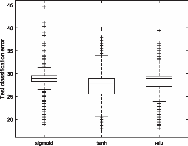
Test classification error for the MovieLens1m data set for predicting gender with the sigmoid nonlinearity (left), the tanh function (middle), and the ReLU nonlinearity (right). ReLU, rectified linear unit.

Considering that ReLUs create sparse models, this result is in line with non-DL prior work,²⁴ which shows that when analyzing high-dimensional behavioral data for predictive purposes, a very large number of the fine-grained behavioral features contribute to the final prediction. Thus, sparse models do not perform as well. Prior work also has reported that for this sort of data, learning linear models with L1-regularization (thus creating sparse models) underperforms modeling with L2-regularization.^45,47 Taken in tandem, these results make sense: L2-regularization is better suited when many features are relevant.⁵¹

Finally, when looking at the effect of the number of hidden layers on the test classification error shown in Figure 6, no consistently better-performing setting can be found for a single data set (MovieLens1m), as well as over all data sets (see the configurations in Table 3). Practitioners should, therefore, test several configurations with a varying number of hidden layers and choose the best-performing architecture.

FIG. 6.

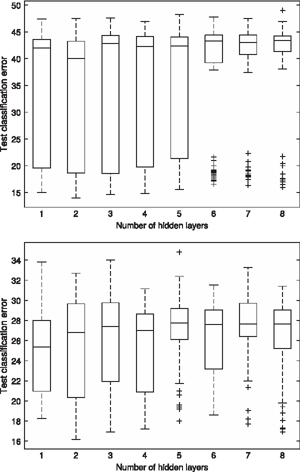
Test classification error for the MovieLens1m data set dependent on the number of hidden layers for predicting age (top) and predicting gender (bottom).

Interpreting deep versus shallow models

In some settings, model comprehensibility is mandatory before a model can be deployed; in others, explaining why the model predicts what it does can help acceptance within an organization.^52–55 One of the advantages of linear shallow classifiers lies in their comprehensibility. The weights given by the model to each of the input features can be inspected and interpreted by humans. Such “global” explanations give insight into how the model works. Instance-level explanations explain why individual cases were classified in a certain way.⁵⁵ For linear models, fast optimal methods exist for explaining the classification of individual instances.⁵⁵

Table 5 lists the features with the highest weights given by LR with L2-regularization for the following classification tasks: predicting (1) gender and (2) age from movie rating data and predicting (3) liberal political beliefs and (4) high intelligence from Facebook like data. A careful interpretation of the features and their relation to the classifications are beyond the scope and purpose of this article. However, we would like to illustrate that despite the inability to simply list out the “most highly weighted” features for the DL models, as we can with linear models, we still have options for interpreting them.

Table 5.

Features with largest coefficients for logistic regression with L2-regularization

Rank	MovieLens (gender)	MovieLens (age)	Facebook (liberal)	Facebook (intelligence)
1.	Ulee's Gold	Scream	Barack Obama	Inception
2.	Starship Troopers	Trainspotting	The Daily Show	The Big Bang Theory
3.	Star Trek: First Contact	I Know What You Did Last Summer	Rent	How I Met Your Mother
4.	Dr. Strangelove	Liar Liar	The L Word	Avatar
5.	Monty Python and the Holy Grail	Pink Floyd—The Wall	Dixie Chicks	Fight Club
6.	In the Name of the Father	Kiss the Girls	Charmed	Star Wars
7.	The Ice Storm	Scream 2	Yoga	TED
8.	Tomorrow Never Dies	Rumble in the Bronx	Amelie	Paulo Coelho
9.	A Clockwork Orange	Spawn	Weeds	Lost
10.	Four Weddings and a Funeral	The Princess Bride	Brokeback Mountain	Music
11.	Six Degrees of Separation	Heathers	Crash	Dexter
12.	The Great Dictator	Monty Python and the Holy Grail	Little Miss Sunshine	The Mentalist
13.	The Blues Brothers	Chasing Amy	The Colbert Report	Sheldon Cooper
14.	The Peacemaker	Mystery Science Theater 3000: The Movie	The Beatles	My Personality
15.	The Abyss	Star Wars	Green Day	The Office
16.	McHale's Navy	Tomorrow Never Dies	Philosophy	Disney's The Lion King
17.	Patton	Willy Wonka and the Chocolate Factory	CNN	Megan Fox
18.	Sphere	Swingers	Sex and the City	Pink Floyd
19.	Apollo 13	Romeo and Juliet	True Blood	Burn Notice
20.	Gattaca	Much Ado About Nothing	Travelling	Futurama

The higher scores indicate higher probability of being (1) male when predicting gender for the MovieLens data set, (2) young when predicting age for the MovieLens data set, (3) liberal when predicting political preference for the Facebook data set, and (4) high IQ when predicting intelligence for the Facebook data set.

Before focusing on the options for the DL models, let us examine the top-weighted features in the LR models. When predicting whether a user is male based on movie-rating data, we can see that higher weights are given to movies that one might suspect were targeted toward male viewers, such as Starship Troopers, Star Trek, and Apollo 13. Looking at the weights that are discriminative for identifying younger viewers, we can see horror movies such as Scream and I Know What You Did Last Summer as well as other movies that it is hard to argue were not target to younger viewers such as The Princess Bride and Willy Wonka and the Chocolate Factory. For the Facebook data set, features such as Barack Obama, The Daily Show, and The Colbert Report are generally associated with a liberal mindset. When predicting whether a user has a high IQ, TV shows such as The Big Bang Theory and Lost receive higher weights.

In contrast to the case with shallow models, the multiple layer nonlinear structure of DL models does not lend itself to direct interpretation. We now demonstrate two approaches to gain insight into the workings of the DL models. First, we can examine some of the neurons in the network, and try to interpret the nuances in the higher level “constructed features” generated from the low-level representation. Second, we illustrate how instance-level explanations can increase understanding of why a DL model classifies individual data instances as it does.

As mentioned previously, the DL models learn distributed representations based on compositionality in the fine-grained features. Each neuron in this multilayered setting assigns weights to lower-level concepts and thus allows for a complex many-to-many combination of all features on different levels. In contrast, shallow techniques such as LR and support vector machines can be viewed as consisting of one neuron, assigning feature weights on one level only (Table 5). To illustrate, Table 6 shows five neurons in the first hidden layer of the best-performing architecture (Table 2) and the features for which they are most activated when predicting gender for the MovieLens1m data set.** At the risk of repeating ourselves, we emphasize that we are not claiming that our interpretation here is in any sense correct, and even where present, any associations between features and classes are statistical not absolute. Our goal is to illustrate the methods: we apply our own interpretation as part of that illustration. (We do assert that a careful research study into the effectiveness of such interpretations for a concrete explanation goal would be valuable.)

Table 6.

Features with largest coefficients for five neurons in the first layer in the deep network for predicting gender on the MovieLens data set

Neuron 1	Neuron 2	Neuron 3	Neuron 4	Neuron 5
The Mirror has Two Faces	McHale's Navy	Kingpin	Apollo 13	Everyone Says I Love You
Bed of Roses	The Blues Brothers	Cool Runnings	Kundun	Little Women
Old YellerKiss the GirlsFly Away HomeThe Adventures of PriscillaTo Kill a MockingbirdMichaelLittle WomenWhen a Man Loves a WomanThe FanRebeccaSome Kind of WonderfulThe PostmanSearching for Bobby FischerStrictly BallroomThe Sound of MusicStand by MeThe ShiningEveryone Says I Love You	Mystery Science Theater 3000: The MovieTomorrow Never DiesStarship TroopersMonty Python and the Holy GrailFour Weddings and a FuneralStar Trek: First ContactApollo 13The Great Dictator12 Angry MenBig NightUlee's GoldSix Degrees of SeparationDuck SoupMaverickDr. StrangeloveVolcanoThe Wedding SingerA Clockwork Orange	Coneheads	Raging Bull	Romeo and Juliet
		Ed	White Squall	The Truth About Cats and Dogs
			Pulp Fiction	The Full Monty
			The Madness of King George	Beauty and the BeastSearching for Bobby FischerThe Sound of MusicThe Mirror has Two FacesBreakfast at Tiffany'sStrictly BallroomStealing BeautyA Christmas CarolSecrets and LiesThe Pillow BookLove JonesMoney TalksInterview with the VampireBed of RosesA Family Thing
			Under Siege
			Ran
			Patton
			The Deer Hunter
			Star Trek: First Contact








Romance, drama	Male, action, comedy	Sport, buddy	Male, drama	Female

Each neuron captures additional fine-grained information. The “cluster names” at the bottom show our interpretation of these neurons, based on the highest weight features.

So, with all of the bias that we bring to the interpretation, each of the five neurons seems to capture a separate nuance of the relationship between movies and gender (see our interpretations in the bottom row of Table 6). Neuron 1 for example captures an aspect of genre by assigning higher weights to romance and drama movies. Neuron 2 focuses on action movies and comedies, which we believe to be favored by male viewers, while neuron 4 discriminates toward “male-oriented” drama movies (more specifically, dramas involving space, war, and other dangerous situations). Neuron 3 becomes active for sport movies, and neuron 5 identifies movies that one might consider to be preferred by female viewers—specifically, movies about love, romance, and relationships, among other things. (Note that Breakfast at Tiffany's and Little Women are explicitly called out in Wikipedia's entry for the “Chick Flick” movie genre; note also the critique of this as a genre, also discussed in the Wikipedia entry.^††)

For the Facebook like data set, Table 7 shows four neurons of the first layer of the deep model for predicting a liberal mindset and the features for which these neurons have high weights. It is unclear here exactly what each neuron might be representing, but they do seem to be grouping “likes” by some sort of similarity. Neuron 1 shows several comedy shows and movies. Neuron 2 has several rock bands (plus Jim Croce, interestingly). Neuron 3 seems to select for hobbies, and Neuron 4 again for rock bands—but of a later era (and Rascal Flatts is a country band).

Table 7.

Top features with highest coefficients for four neurons in the first layer in the deep network for predicting a liberal mindset from the Facebook data set

Neuron 1	Neuron 2	Neuron 3	Neuron 4
Gilmore Girls	Two and a Half Men	Cooking	Green Day
Travel	AFI	Heroes	Oasis
Matchbox 20	Kings of Leon	Reading	Rascal Flatts
Grey's AnatomyCounting CrowsSeinfeldFerris Bueller's Day OffCoyote UglyNapoleon DynamiteSex and the City	Iron MaidenNip/TuckJim CroceGuns N’ RosesLed Zeppelin	Summer NightsMusicWritingLaughing	IncubusFear and Loathing in Las VegasFall Out Boy
Largely Comedies	Largely Rock Bands	Hobbies	Largely Rock Bands

Each neuron captures additional fine-grained information (our interpretation, bottom row).

Despite the possibility that such interpretations are meaningful, especially with the latter example, we do not get a good idea of why these neurons would be helpful for predicting the target variable—liberal mindset. Also, this approach becomes infeasible when a much larger number of neurons are present.²⁸ Moreover, it is insufficient to only interpet first-layer neurons as higher-level concepts are derived from lower-level concepts, and the cascading nonlinearities are not addressed by this sort of explanation. That being said, these examples illustrate that deep architectures capture potentially complex concepts, with more structure and nuance than we see with linear models.

Another approach to disentangle the inner workings of deep classification models is by examining instance-level explanations.⁵⁵ Global explanations are particularly challenging for ultrahigh-dimensional behavioral data. But the sparseness of the data provides an advantage when examining instance-level explanations. If we care about what is there in the data that leads the model to classify as it does, we can look specifically for counterfactual explanations of the classification,^46,55,56 which report those features that cause the network to classify the instance as it does. An instance-level counterfactual explanation is a minimal (irreducible) set of features such that removing those features would change the predicted class of that specific instance.

Carefully examining instance-level explanations for deep-learned networks from behavioral data is beyond the scope of this article (and would be a very interesting article in itself). However, it is straightforward to show what such explanations would look like. Consider the Facebook like data. An instance-level explanation will focus on explaining why a certain Facebook user is classified as a specific class of interest (e.g., “high intelligence” or “female”). As an illustration, Figure 7 shows the reason why a certain instance (Facebook user Julie in our example) is classified as highly intelligent: if Julie would not have liked “Antwerp.ai,” “Cowspiracy,” and “Black Mirror,” then her predicted class would change from highly intelligent to medium intelligent. In other words, if the data for Julie had not contained likes for these pages, her predicted class would not have been “high intelligence.” Note that we follow the procedure described by Martens and Provost⁵⁵ to generate explanations.

FIG. 7.

Example explanation why Facebook user Julie is classified as highly intelligent.

As explained in detail by Martens and Provost,⁵⁵ there are many reasons why explanations are necessary for data-driven decision-making systems. For example, automated decision-making systems often need to be justified to the stakeholders who will approve their use. Particular decisions may be called into question and, therefore, need to be explained. Machine learning engineers may need to improve or debug a deployed system. In all these situations, explanations for decisions can be substantially informative. A careful study of explanation approaches for DL from large sparse behavioral data is an important topic for future research.

Why DL performs well

Finally, to gain added insight into why DL works well on behavioral big data, we now demonstrate the added value of the deep models' distributed feature representation. Recall that previously we discussed how learning unsupervised distributed feature representations has been shown not to be helpful for improving LR models. DL learns a distributed representation (the first layer of the deep architecture). However, the backpropagation through the deep architecture means that the distributed representation learning is supervised. Thus, it may be that the distributed representation learned at the first layer is the main source of the power of the DL.

To examine how much value is provided by the supervised learning of a distributed representation for the sparse raw features, we transform the original highdimensional data sets onto three reduced-feature data sets and assess their prediction capability. More specifically, we build an LR-BGD from each reduced feature space. We compare the following three models: 1.

An LR-BGD model where the features are the first-layer distributed features learned by DL (Table 2).

An LR-BGD model that uses L1-regularization to identify relevant features, with the regularization parameter set in the same way as with LR-BGD-L2 mentioned previously. A feature with a corresponding nonzero weight thus is being used by the model.

An LR-BGD model that uses as features the distributed representation created through SVD. This representation is similar to that created by DL, but learned without referencing the target variable (i.e., unsupervised).^‡‡ For this experiment, we chose the same number of SVD dimensions as first-layer DL features in the DL architecture (Table 2).

The results of this analysis are given in Table 8. Among the three alternative LR methods, the method with the largest AUC is shown in bold. For 33 out of 39 data sets, the latent features learned by DL result in better predictive performance than the selected or latent features resulting from the other two approaches. This demonstrates the value of the distributed representations learned by DL in a supervised manner, and gives preliminary insight as to why DL techniques perform well on behavioral big data.

Table 8.

Area under the ROC curve reached with logistic regression (LR; rightmost three columns) by transforming the original high-dimensional datasets onto a reduced feature set by taking the first-layer neurons as features for the LR (DL-layer1-LR), by applying feature selection through L1-regularization (L1-LR), and by creating an unsupervised distributed representation through singular-value decomposition-LR

Data set	DL	DL-layer1-LR	L1-LR	SVD-LR
BookCrossing	55.32	54.37	52.24	51.60
Facebook_swl	55.67	54.21	51.64	50.87
TaFeng	71.35	64.43	60.62	63.32
YahooMovies_age	65.66	61.44	57.91	55.13
Fraud	77.22	72.9	53.49	58.40
Car	78.16	61.43	54.99	58.65
MovieLens_adventure	78.61	50.09	57.50	54.54
MovieLens_100k_gender	79.30	72.83	61.55	65.35
Ecommerce	76.34	75.05	57.12	58.15
MovieLens_crime	79.86	56.78	52.71	51.92
Facebook_female_gay	77.98	63.09	60.56	59.88
MovieLens_fantasy	80.83	67.09	50.00	56.28
MovieLens_mystery	80.65	80.44	78.55	79.77
YahooMovies_gender	81.35	77.35	66.89	70.86
MovieLens_romance	81.75	73.1	55.74	50.70
MovieLens_thriller	84.21	85.40	72.22	72.93
MovieLens_drama	84.72	58.89	54.11	58.34
KDD2015	85.26	60.67	62.99	61.64
MovieLens_children	85.46	73.72	70.76	69.72
MovieLens_1m_gender	85.63	78.52	74.10	78.14
MovieLens_comedy	87.04	57.28	59.19	54.38
Flickr	87.45	73.46	54.60	57.13
MovieLens_action	87.79	59.53	59.49	55.62
MovieLens_animation	88.31	70.41	62.67	60.69
MovieLens_scifi	89.08	87.19	50.00	68.07
MovieLens_100k_age	89.50	84.91	75.95	81.61
MovieLens_documentary	90.04	63.61	54.52	59.09
MovieLens_western	90.72	82.87	67.21	57.44
MovieLens_1m_age	91.39	86.57	82.00	85.04
Facebook_religion	92.02	82.33	75.44	78.09
MovieLens_horror	92.42	69.26	58.50	58.00
Facebook_male_gay	91.78	82.44	81.09	81.32
MovieLens_filmnoir	90.12	59.51	62.25	53.52
Facebook_political	93.63	77.60	78.22	77.11
Facebook_IQ	94.40	85.99	80.33	62.09
MovieLens_musical	95.02	77.50	76.58	86.64
Facebook_gender	93.47	88.54	62.89	61.23
MovieLens_war	95.45	90.97	54.02	53.97
LibimSeTi	99.69	97.24	97.22	97.20

Bold indicates the highest achieved AUC for that dataset by the reduced feature sets (excluding the DL model built from the original, high-dimensional dataset).

These are compared here with the AUCs with the full DL.

SVD-LR, singular-value decomposition-logistic regression.

However, as given in Table 8, for every single data set the prediction capability of the entire DL model remains higher than using any of the reduced-dimensionality feature sets. For this reason, we conclude that the higher layers in the deep architectures add considerable value for modeling the complex nonlinear dependencies present among the independent behavioral features.

In addition, when comparing the performance of the model built from the DL first-layer neurons against the full LR-BGD-L2 model (Table 3), we observe that the full LR-BGD-L2 model outperforms the reduced feature model (in terms of AUC), which is in line with prior findings.⁴⁷ Nevertheless, these results suggest further research directions in terms of using the distributed nature of first-layer neurons (and by consequence, higher-level neurons) for purposes of feature engineering. For example, typically tree-structured models do not work well for this sort of data, due to the extremely high dimensionality and need for nonsparse models. However, what about an ensemble of trees built on the deep-learned distributed representation?

Conclusion

In the past, DL has shown significant performance improvements for tasks from image classification, speech recognition, and natural language processing. This article performs a detailed study examining whether these improvements also extend to behavioral big data. We demonstrate the usefulness of the supervised learning of deep distributed representations of fine-grained behavioral features, while shedding light onto when and why DL performs well and how these models might be interpreted. As a practical contribution, we provide guidance regarding favorable HP configurations for learning these models.

A head-to-head comparison between DL and LR shows that DL achieves a statistically significant performance improvement over well-regularized LR. However, in a less rigorous comparison with shallow techniques beyond LR, although DL still comes out on top, in many cases the marginal improvements of the more complex models overall are quite small. Investigating when DL performs better, the results suggest that DL is not better in problem settings where the data are characterized by low SNS separability. This line of inquiry requires further research.

To (partially) open up the black box, we first investigate the distributed representations learned by the deep models and illustrate how the nuances captured by first-layer neurons can be interpreted. Although not all neurons are easily interpretable and domain knowledge is needed, this demonstration suggests directions for further research. Moreover, it provides an avenue for decision makers to obtain insight and intuitions into the lowest level of the behavioral hierarchy. Second, we suggest instance-level explanations for interpreting deep models as an approach worth exploring in future research.

The distributed and nonlinear nature of deep models may explain why DL works well on complex behavioral data. More specifically, we demonstrate that the first-layer features learned in a supervised manner by DL yield higher prediction accuracy (AUC) than other methods for reducing features (yet not as high as well-regularized LR using the full shallow feature set). This supports the added value of supervised learning of distributed representations for behavioral data.

On a more practical level, we have tried to provide insight into the implementation characteristics of DL on behavioral data. The multitude of HPs can be overwhelming for researchers and practitioners when applying DL for this or any new application. Two HPs are found consistently to achieve better results. First, dense representations throughout the models achieve better predictive performance, more specifically by employing tanh activation functions. Second, using an unsupervised pretraining phase does not improve performance in this discriminative setting. Apparently, unlike in tasks such as object recognition, the input variations learned through the pretraining phase do not contribute substantially to the final classification task. This can be due to an inappropriate underlying generative process, not tailored toward human behavioral data and/or the subsequent prediction task. Another explanation is that the unsupervised learning cannot efficiently grasp the important variations in the complex data without taking into account the target variable. Future research could focus on developing an unsupervised generative process that fits the process of human-generated behavior better. However, since the target variable is often not clearly related to the input data, it seems worthwhile to focus on supervised pretraining, so that input data variations can be explicitly related to the variable of interest.

This article demonstrates the usefulness of DL for behavioral big data and underlines its potential in future applications with this type of data. The performance improvements must be considered in tandem with the drawbacks in terms of additional computational and implementational complexity. This hurdle might currently render them infeasible in a practical setting—for our results it often took multiple days for training on the very fine-grained data sets. As the availability of GPU units on cloud computing instances becomes more widespread and Theano's support for multiple GPU use becomes less experimental, the computation time could be improved substantially. (One still must consider paying for this computation.) In contrast, in practice big behavioral data may be much larger than the data sets analyzed in this article—which will make DL methods even harder to apply, but also may render them more accurate, as the relative performance of linear and nonlinear methods is critically related to the amount of training data.⁴⁸ As a future study, it would be interesting to see a learning curve analysis to see whether we might expect substantial increases in generalization performance with DL for high-dimensional sparse behavioral data (cf. the usual learning curve performance of shallow learning on such data²⁴).

Footnotes

Author Disclosure Statement

No competing financial interests exist.

Funding Information

Sofie De Cnudde and Yanou Ramon thank the Research Foundation-Flanders for supporting this research. Sofie De Cnudde has received funding from the Research Foundation-Flanders under the Grant number G031914. Yanou Ramon has obtained a PhD Research Fellowship from 2018–2022.

Foster Provost thanks Andre Meyer for a Faculty Fellowship and the NYU/Stern Fubon Center for supporting research in Data Analytics and AI.

Abbreviations Used

Appendix

References

Ciresan

, Meier

, Schmidhuber

Multi-column deep neural networks for image classification. In: IEEE Conference on Computer Vision and Pattern Recognition (CVPR). Rhode Island: IEEE, 2012. pp. 3642–3649.

Krizhevsky

, Sutskever

, Hinton

. Imagenet classification with deep convolutional neural networks. In: Advances in neural information processing systems. Lake Tahoe, NV, 2012. pp. 1097–1105.

Ciresan

, Meier

, Masci

, et al. Flexible, high performance convolutional neural networks for image classification. In: JCAI Proceedings-International Joint Conference on Artificial Intelligence (IJCAI), vol. 22. Barcelona, Spain, 2011. p. 1237.

Sutskever

, Vinyals

, Le Quoc

Sequence to sequence learning with neural networks. In: Advances in neural information processing systems (NIPS). Montreal, Canada, 2014. pp. 3104–3112.

Huang

P-S

, He

, Gao

, et al. Learning deep structured semantic models for web search using clickthrough data. In: Proceedings of the 22nd ACM international conference on Conference on information & knowledge management. San Francisco, CA, 2013. pp. 2333–2338.

LeCun

, Bengio

, Hinton

. Deep learning. Nature. 2015; 521:436–444.

Deng

Three classes of deep learning architectures and their applications: A tutorial survey. In: APSIPA transactions on signal and information processing. Cambridge, UK: Cambridge University Press, 2012.

, Sheridan

, Liaw

, et al. Deep neural nets as a method for structure–activity relationships. J Chem Inf Model. 2015; 55:263–274.

Dahl

, Jaitly

, Salakhutdinov

. Multi-task neural networks for QSAR predictions. 2014. arXiv preprint arXiv:1406.1231.

10.

Ramsundar

, Kearnes

, Riley

, et al. Massively multitask networks for drug discovery. 2015. arXiv preprint arXiv:1502.02072.

11.

Chicco

, Sadowski

, Baldi

Deep autoencoder neural networks for gene ontology annotation predictions. In: Proceedings of the 5th ACM Conference on Bioinformatics, Computational Biology, and Health Informatics. Newport Beach, CA, 2014. pp. 533–540.

12.

Salakhutdinov

, Mnih

, Hinton

. Restricted Boltzmann machines for collaborative filtering. In: Proceedings of the 24th international conference on Machine learning. Corvallis: Oregon State University. 2007. pp. 791–798.

13.

Van den Oord

, Dieleman

, Schrauwen

Deep content-based music recommendation. In: Advances in neural information processing systems. Lake Tahoe, NV, 2013. pp. 2643–2651.

14.

Glorot

, Bengio

. Understanding the difficulty of training deep feedforward neural networks. AISTATS. 2010; 9:249–256.

15.

Shmueli

Research dilemmas with behavioral big data. Big Data. 2017; 5:98–119.

16.

, Zhu

, Wu

G-Q

, et al. Data mining with big data. Trans Knowl Data Eng. 2014; 26:97–107.

17.

Kosinski

, Stillwell

, Graepel

. Private traits and attributes are predictable from digital records of human behavior. Proc Natl Acad Sci U S A. 2013; 110:5802–5805.

18.

Martens

, Provost

, Clark

, et al. Mining massive fine-grained behavior data to improve predictive analytics. MIS Q. 2016; 40:869–888.

19.

Liu

, Dolan

, Pedersen

. Personalized news recommendation based on click behavior. In: International Conference on Intelligent User Interfaces (IUI). Hong Kong, China, 2010. pp. 31–40.

20.

, Du

T.C

. Building a targeted mobile advertising system for location-based services. Decis Support Syst. 2012; 54:1–8.

21.

Tobback

, Martens

. Retail credit scoring using fine-grained payment data. J R Stat Soc A (Stat Soc). 2019.

22.

Verbeke

, Martens

, Baesens

. Social network analysis for customer churn prediction. Appl Soft Comput. 2019; 14:431–446.

23.

Junqué de Fortuny

, Stankova

, Moeyersoms

, et al. Corporate residence fraud detection. In: International Conference on Knowledge Discovery and Data Mining (SIGKDD). New York, NY. 2014. pp. 1650–1659.

24.

Junqué de Fortuny

, Martens

, Provost

. Predictive modeling with big data: Is bigger really better?. Big Data. 2013; 1:215–226.

25.

Junqué de Fortuny

, Martens

, Provost

. Wallenius Bayes. Mach Learn. 2013; 107:1013–1037.

26.

Cortes

, Vapnik

. Support vector machine. Mach Learn. 1995; 20:273–297.

27.

Bengio

Learning deep architectures for AI. Found Trends Mach Learn. 2009; 2:1–127.

28.

Hinton

. Distributed representations. Cambridge, MA: MIT Press. 1986.

29.

Rokeach

. Understanding human values: Individual and societal. New York (N.Y.): Free Press. 1979.

30.

Zeiler

, Fergus

Visualizing and understanding convolutional networks. In: European Conference on Computer Vision. Zurich, Switzerland: Springer, 2014. pp. 818–833.

31.

Arras

, Horn

, Montavon

, et al. “What is relevant in a text document?”: An interpretable machine learning approach. CoRR. 2016; abs/1612.07843.

32.

JV.

Advantages and disadvantages of using artificial neural networks versus logistic regression for predicting medical outcomes. J Clin Epidemiol. 1996; 49:1225–1231.

33.

Livni

, Shalev-Shwartz

, Shamir

On the computational efficiency of training neural networks. In: Advances in Neural Information Processing Systems (NIPS). Montréal, Canada, 2014. pp. 855–863.

34.

Vieira

. Predicting online user behaviour using deep learning algorithms. 2015. arXiv preprint arXiv:1511.06247.

35.

Bergstra

, Bengio

. Random search for hyper-parameter optimization. J Mach Learn Res. 2012; 13:281–305.

36.

Hinton

A practical guide to training restricted Boltzmann machines. Momentum. 2010; 9:926.

37.

Provost

, Fawcett

. Data science for business: What you need to know about data mining and data-analytic thinking. Sebastopol, CA: O'Reilly Media Inc., 2013.

38.

Goodfellow

, Bengio

, Courville

. Deep learning. Cambridge, MA: MIT Press. 2016.

39.

Fawcett

An introduction to ROC analysis. Pattern Recogn Lett. 2006; 27:861–874.

40.

Erhan

, Bengio

, Courville

, et al. Why does unsupervised pre-training help deep learning?. J Mach Learn Res. 2010; 11:625–660.

41.

Bergstra

, Breuleux

, Bastien

, et al. Theano: A CPU and GPU math expression compiler. In: Proceedings of the Python for Scientific Computing Conference (SciPy). Austin, TX. 2010.

42.

Hinton

, Osindero

, Teh

Y-W

. A fast learning algorithm for deep belief nets. Neural Comput. 2006; 18:1527–1554.

43.

Glorot

, Bordes

, Bengio

Deep sparse rectifier neural networks. In: Proceedings of the Fourteenth International Conference on Artificial Intelligence and Statistics. Fort Lauderdale, FL: JMLR.org, 2011. pp. 315–323.

44.

Masters

, Luschi

. Revisiting Small Batch Training for Deep Neural Networks. 2018. CoRR. abs/1804.07612.

45.

De Cnudde

, Martens

, Provost

, et al. A benchmarking study of classification techniques for large, behavioral data. Int J Data Sci Anal. 2019; 7:1–43.

46.

Chen

, Fraiberger

, Moakler

, et al. Enhancing transparency and control when drawing data-driven inferences about individuals. Big Data. 2019; 5:197–212.

47.

Clark

, Provost

. Unsupervised dimensionality reduction versus supervised regularization for classification from sparse data. Data Mining Knowl Discov. 2019.

48.

Perlich

, Provost

, Simonoff

. Tree induction vs. logistic regression: A learning-curve analysis. J Mach Learn Res. 2003; 4:211–255.

49.

Demšar

Statistical comparisons of classifiers over multiple data sets. J Mach Learn Res. 2006; 7:1–30.

50.

Hand

DJ.

Classifier technology and the illusion of progress. Stat Sci. 2006; 21:1–14.

51.

AY.

Feature selection, L1 vs. L2 regularization, and rotational invariance. In: Proceedings of the Twenty-First International Conference on Machine learning. New York, 2004. p. 78.

52.

Gönül

, Önkal

, Lawrence

. The effects of structural characteristics of explanations on use of a DSS. Decis Support Syst. 2006; 42:1481–1493.

53.

Gregor

, Benbasat

. Explanations from intelligent systems: Theoretical foundations and implications for practice. MIS Q. 1999; 497–530.

54.

Martens

, Baesens

, Van Gestel

, et al. Comprehensible credit scoring models using rule extraction from support vector machines. Eur J Oper Res. 2007; 183:1466–1476.

55.

Martens

, Provost

. Explaining data-driven document classifications. MIS Q. 2014; 38:73–99.

56.

Provost

. Understanding decisions driven by big data: From analytics management to privacy-friendly cloaking devices. Keynote Lecture, Strata Europe. 2014.