The Pearls and Perils of Google Trends: A Housing Market Application

Abstract

This study aims at providing insights into the correct usage of Google search data, which are available through Google Trends. The focus is on the effect of sampling errors, which has not received the attention that it deserves. A housing market application is used to demonstrate the effects. For this purpose, the relationship between online search activity for mortgages and real housing market activity is investigated. A simple time series model, which explains transactions by an online mortgage search, is estimated. The results show that the effect of sampling errors is substantial. Thus, although the application of Google Trends data in research remains promising, far more attention should be given to the limitations of these data.

Introduction

Google Trends is one of the most accessible gateways to big data there is available. It transforms global search queries from Google's own search engine into small aggregated datasets or visualizations, thereby providing insights into the popularity of specific queries. Since the introduction of Google Trends in the summer of 2008,¹ it has provided access to big data for many users. Its user-friendly portal has aided in its popularity. The aggregated Google search queries, based on individual search behavior, have been applauded widely and have also found their ways into many academic disciplines; applications include, for instance, economics, health care, and tourism.^2–4

Google Trends data, however, come with important limitations. The most important of all, as noted by Nuti et al., is the “lack of detailed information on the method by which Google generates this search data” (p.46).⁵ Although they make it evident that the lack of documentation by researchers themselves is highly problematic for reproducibility of the research, they do conclude that the larger limitations remain “in the Google Trends tool itself” (p.46). This article focuses on the data provided by Google Trends. I will concentrate on what I consider to be the most important limitation of all: sampling error.

The existence of sampling error in Google Trends data is not a new observation. It has been mentioned, for instance, by Choi and Varian in 2012.⁶ It is often suggested, however, that the sampling error may be ignored,⁷ with the most notable exceptions being Greenwood-Nimmo and Shields and Carrière-Swallow and Labbé.^8,9 Nevertheless, the number of studies that either use oversimplified measures to suggest moderate sampling effects^10–12 or revert to faulty solutions altogether^13,14 are on the rise. This article, thus, argues that sampling error is not receiving the consideration that it deserves.

The article investigates the extent to which sampling error can affect research outcomes. I use a housing market application to illustrate the problem and demonstrate the effects of sampling error in estimation. Housing market applications of Google search queries include Choi and Varian, Wu and Brynjolfsson, and Van Veldhuizen et al.^15–17 In this article, the results of multiple sampling are compared with a one-sample study; Van Veldhuizen et al. is used for this because of its reproducibility.¹⁷ I make the case that the sampling issues should be addressed separately from the estimation techniques that researchers may employ. After all, when measurement error leads to inconsistent parameter estimates, the obvious thing, according to Pischke, is to: “Get better data” (p.4).¹⁸ Therefore, this study does not focus on forecasting or nowcasting, which are the main applications of the Google Trends data in research, but on the data itself.

The study thereby provides insights into the correct usage of Google Trends. The article demonstrates that disregarding sampling error leads to overstating the importance of Google Trends data in the prediction of housing market transactions, indicating the risks of publication bias. Nevertheless, including Google Trends data can still lead to a modest improvement compared with a benchmark model where online search activity is ignored. The article contributes to the literature on applying big data sources in academic research. Particularly, the article adds insights to housing market applications. More than any other housing market study, it stresses the limitations in using these data.

The rest of this article is organized as follows. The Literature section provides an overview of the Google Trends literature with a focus on sampling errors. The Data section describes the Google Trends data that are used in the article as well as the housing market data. The Methodology section introduces the methodology of the housing market application. The Results section presents the estimation results. The Conclusion section summarizes and concludes the article.

Literature

There is a substantial body of literature on Google Trends.^1,6–8,16 However, this does not imply that there is detailed information on Google's methodology in generating the data.^1,5 Its exact functioning remains undocumented and caution is thus necessary when working with Google Trends data. Still, according to Choi and Varian, “queries can be useful leading indicators” (p.2; emphasis theirs).⁶ In the words of Askitas, it is just that Google Trends data are “in need of the right question” (p.1).¹

Limitations and biases

Google Trends data contain important limitations and biases. First, the data are based on search queries by using Google's search engine only. Selection bias may, thus, be an issue if search behavior is correlated with search engine preferences or Internet use in general. Lower levels of Internet penetration in emerging markets will, for instance, make Google Trends indices less representative for its population.⁹ To increase representativeness of the data, at least to a certain extent, Google makes use of a “sessionization” approach, which counts multiple searches by an individual within a 24-hour period as one search only.¹

Second, Google Trends indices make use of threshold values. If the number of searches in a given time period is too small, that is, if the threshold is not met, then the index value is set to zero. These threshold values are not reported by Google.^7,8 Zero values may, thus, be actual zeros or censored observations. Indices for queries with low absolute search numbers will, thus, lead to less reliable time series. A similar problem is caused by the rounding to the nearest integer.⁷ As by construction the Google Trends values range from 0 to 100, growth rates calculated from low observed values will contain particularly large errors.

Third, Google uses a sampling procedure to generate Google Trends indices. Information on the sample size is not disclosed by Google.¹ A complication herein is that new samples can be taken only once per day as data are cached by Google on a daily basis only.⁷ Google Trends, thus, uses a different sample to generate the index on every single date.¹⁹ An identical query on Google Trends will, thus, lead to the exact same time series when done on the same day but to a different series when obtained on a different date.^* Therefore, as noted by Stephens-Davidowitz and Varian, “A researcher who wants to average multiple samples must wait a day to get a new sample” (p.13).⁷

Finally, little is known on the algorithms used by Google. Recommended searches of the Google search engine may, for instance, affect outcomes.²⁰ Algorithm uncertainty also applies, to different extents, to sessionization, threshold values, and the sampling procedure. As noted by Andreano et al., the sampling design is “completely unknown” (p.182).¹⁴ Even larger risks apply when Google starts “helping” in analyzing the data. This is, for instance, the case when the Google Trends’ categorization options are used: Google Trends provides predefined categories such as Science, Health, and Travel. Askitas remarks, using a labor market example, that searches on Steve Jobs may be excluded automatically from the query results for “jobs” when the category is set to Classifieds.¹ However, he also notes that no information is provided on how these categories are defined.

Lazer et al. note that the categorization algorithms are highly susceptible to algorithm dynamics, such as “changes made by engineers to improve the commercial service” (p.1204), and they demonstrate these risks for the discontinued Google Flu Trends.²⁰ Google Flu Trends was a separate service offered by Google, aiming at predicting influenza outbreaks, and it should not be confused with Google Trends.

Sampling error

In this subsection, the earlier mentioned sampling error in Google Trends data will be discussed in more detail. The sampling error in Google Trends data occurs, because Google uses only “a percentage of searches” to compile the index.²¹ What percentage that might be, or whether it is even constant, is unclear. A rare indication of the sample size might be given by Hal Varian, who coauthored one of the earliest Google Trends papers¹⁵: “At Google, for example, I have found that random samples on the order of 0.1 percent work fine for analysis of business data” (p.4).²² It is the only indication of the potential sample size that I am aware of.

The unknown sampling procedure and the, at least in relative terms, small sample size that is used to generate Google Trends indices raise questions about the validity of the Google Trends data. Nevertheless, scholars have not given sampling error in Google Trends data the attention that it deserves. This can partly be attributed to Stephens-Davidowitz and Varian who, in their “Hands-on Guide to Google Data,” have stated that they “do not expect that […] researchers will need more than a single sample” (p.13).⁷ This current article stresses that such a general claim cannot be made, as Google Trends indices depend on the chosen query, the geography, and time span. Indices for more popular search terms, more populous regions, and higher time aggregation (i.e., monthly observations instead of weekly or daily ones) are expected to have smaller sampling errors.

It turns out that the variability in the number of samples used by researchers using Google Trends data is considerable. The same has to be said about disclosing this information. To illustrate: Wu and Brynjolfsson do not provide the necessary information but there is no reason to assume that more than one sample is used.¹⁶ A little more evidence that only one sample is used can be found in, for instance, the work of Choi and Varian.⁶ Van Veldhuizen et al. and Silva et al. are other examples of studies relying on one sample only.^17,23

Da et al. download an index “several times” (p.1467) but use only one of them in estimation.¹⁰ Similarly, Chauvet et al. make downloads “several different days” (p.8) but rely on only one of the samples.¹¹ Kearney and Levine take samples “multiple times” (p.3619) and use the average.²⁴ These aforementioned studies all exhibit what Nuti et al. describe as “poor documentation of methods” (p.46) by researchers using Google Trends.⁵

More information is provided, generally, by those studies that rely on multiple samples. For instance, Preis et al. retrieve Google Trends data “on 10 April 2011, 17 April 2011, and 24 April 2011” (p.5).² McLaren and Shanbhogue rely on “a more stable data set by taking the average of the data generated on seven consecutive days” (p.135).¹⁹ Seabold and Coppola download data “for ten days over a period of one month” (p.6) and use the average as an approximation.²⁵

Greenwood-Nimmo and Shields use 30 different downloads “each of which was downloaded on a different day between 6 March 2015 and 15 May 2015” (p.366).⁸ They use the samples to determine the median, as it is less sensitive to outliers. Carrière-Swallow and Labbé “download the series for each keyword on 50 occasions” (p.291) to construct averages for their percentage change variables.⁹

The use of more samples comes with a “substantial time-cost associated with collecting the data as each draw is obtained on a separate day” (p.371); still, Greenwood-Nimmo and Shields consider their 30 samples a compromise in this regard.⁸ Further, it should be noted that researchers who collect more samples do, indeed, observe substantial sampling variation. In the words of Seabold and Coppola: “the sampling error is evident” (p.6),²⁵ whereas according to Greenwood-Nimmo and Shields: “variation across draws is non-negligible in all cases” (p.366).⁸

A recurring argument used by scholars who download more than one sample but use only one in estimation is that the correlation between the time series downloaded on different days is high. Da et al., the first to use the argument, observe that the correlations between the Google Trends indices that were downloaded “several times […] are usually above 97%” (p.1467).¹⁰ Nevertheless, high cross-correlations between time series downloaded on different days do not provide sufficient evidence to conclude that sampling error is irrelevant.^† Still, the simplicity of the argument used by Da et al. seems to have led to a wider use. The argument can, for instance, be found in Chauvet et al.¹¹ and, largely verbatim, in Markiewicz et al.¹²

These three studies have in common that they assume that high correlations between series imply that the results will be the same if a different sample would be used. In the words of Da et al.: “We believe that the impact of such sampling error is small for our study and should bias against finding significant results” (p.1467; emphasis mine).¹⁰

A false solution to obtain more samples, and thus mitigate the sampling problem, has been suggested by D'Amuri and Marcucci.¹³ They claim that Google Trends indices do not only change daily but also change “with the IP address” (p.804).¹³ Consequently, they claim to use 24 samples that are downloaded on “12 different days from two different IPs” (p.804).¹³ Samples, however, do not structurally differ between IP addresses, all else equal. As indicated by, for instance, McLaren and Shanbhogue, Choi and Varian, and Stephens-Davidowitz and Varian queries done on the same day lead to the same series as the data are cached or stored.^6,7,19

Indeed, the descriptive statistics of the raw Google Trends data used by D'Amuri and Marcucci, see their Supplementary Data (pp.11–13),¹³ show clearly that most of the monthly series from the first IP address correspond with the series of the second IP address on a different date.^‡ Regrettably, Andreano et al. pick up on the fallacy introduced by D'Amuri and Marcucci and contribute further to its spread: “Given the sampling approach of Google, downloading the series from multiple IP addresses over a short time period, and getting the average, seems a preferable solution” (p.184).¹⁴ I consider this an illustration of the potentially hazardous consequences of the lack of documentation when it comes to Google Trends data.⁵

Data

Google Trends data

The Google Trends data that are used in the analysis are obtained from https://trends.google.com/trends/. From the website the data can be downloaded as a CSV file. The data are presented as an index that provides the relative popularity of queries from the Google search engine; that is, the popularity of a query is expressed relative to the total number of searches from the same period and region. The period in which the relative popularity of a given query is highest is set to 100. The other periods are expressed relative to this maximum, resulting in index values in the range 0–100.^8,19

For the housing market application in this paper, online search data for the Dutch word for mortgage, that is, the query hypotheek, are used. The Google Trends data have been restricted to include only searches from the Netherlands. Practically all Dutch households (i.e., 97%) had broadband Internet access in 2018. The Netherlands, thereby, ranked first in the EU (pp.71–72).²⁷ The 100 samples of the monthly time series were taken on 100 consecutive days between January 25, 2018 and May 4, 2018. The time series started in January 2004, that is, the earliest possible, and continue to the latest data that were available at the time of collection. Finally, it should be noted that at present Google Trends provides monthly data for periods longer than 5 years whereas in the past Google Trends provided weekly series only.¹⁹

Figure 1 illustrates the sampling error of the mortgage query by plotting the minimum and maximum values for each month between 2004 and 2018 for the 100 samples, taken on 100 consecutive days starting on January 25, 2018. It should be noted that all index values are larger than 40; that is, the aforementioned threshold values are of no concern for these data. In the figure, different sample sizes are superimposed, demonstrating that the min–max range increases with the number of samples.

FIG. 1.

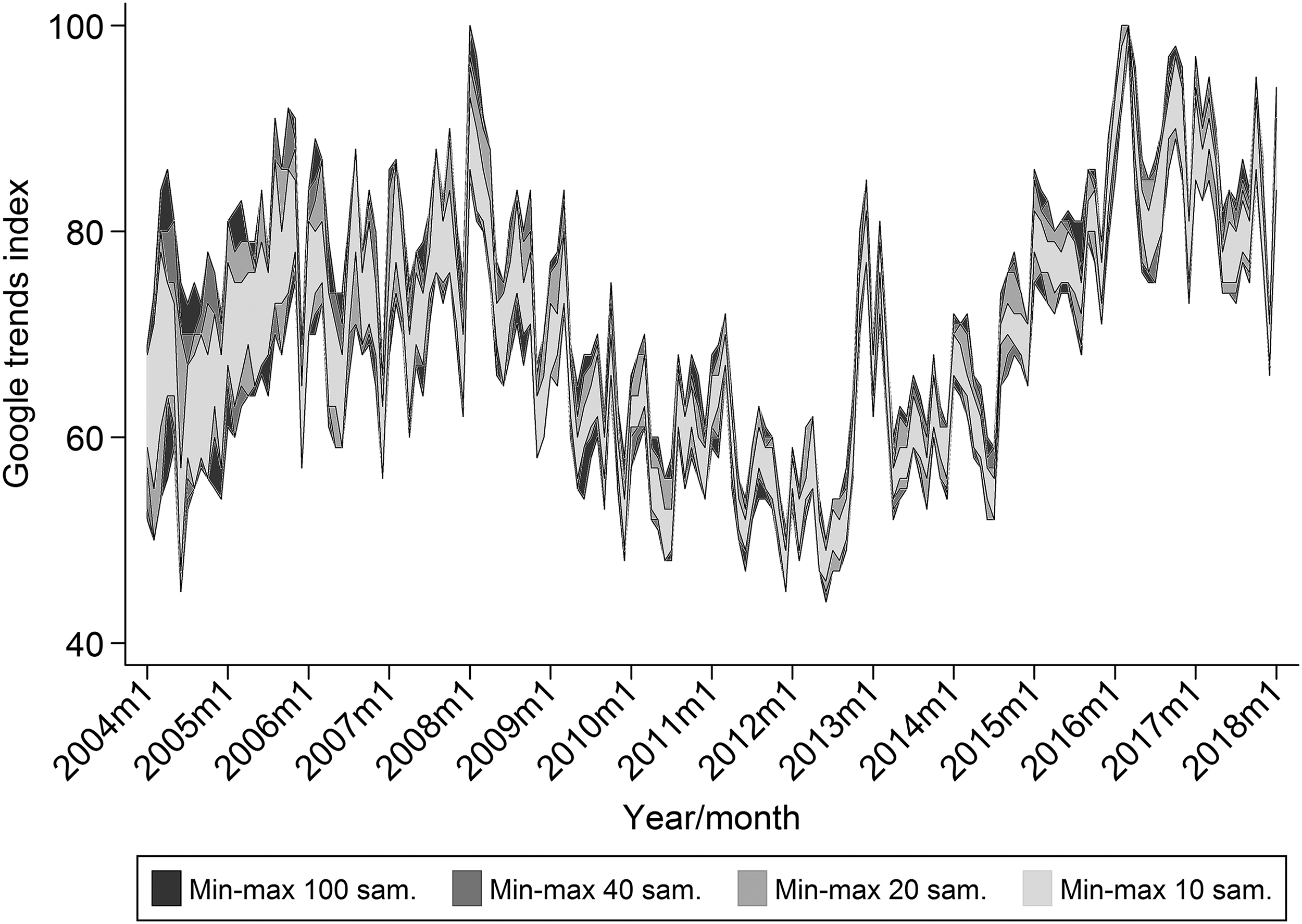
Min−max range for up to 100 Google Trends samples, queries for mortgages in the Netherlands.

Between January 2004 and January 2018, the min–max range varies between 30 index points (March, April and June 2004) and 2 index points (March 2016) or, in relative terms, between 66.7% (June 2004) and 2.0% (March 2016). Figure 1 indicates that the sampling error is substantial. The effects of these sampling errors will be investigated in the Results section.

Housing transaction data

In addition to the Google Trends data, transaction data are required for the housing market application. Following Van Veldhuizen et al., transaction data based on the Cadastre records will be used.¹⁷ These aggregated data are publicly available at Statistics Netherlands.^28,29 The transaction data are based on the date of conveyance (completion), the date at which ownership is transferred from one party to the other. Importantly, the date at which the final offer is accepted, which is legally binding in the Netherlands, and the date at which the purchase contracts are signed precede the date of conveyance.

To illustrate the issue, Figure 2 depicts the time between the conveyance date and the closing of the listing by the realtor, which generally is the date the purchase contract is signed, using non-public microdata from Statistics Netherlands (CBS) and the Dutch Association of Realtors (NVM). The sample consists of transaction data for 584,923 family homes between January 2004 and August 2013. The figure illustrates that, in general, the purchase date does not coincide with the conveyance date. On average the difference is about 3 months, as is the median. These statistics correspond with a descriptive study done by Kadaster and NVM, which indicates a “conveyance period” of 3.1 months for 23,000 transactions, between 1994 and 2017, in the Municipality of Zwolle.³⁰

FIG. 2.

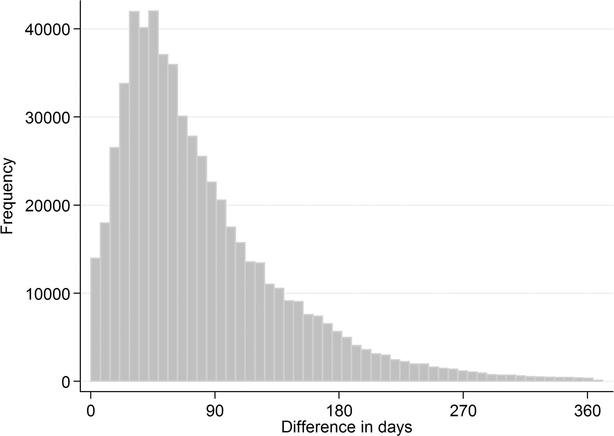
Days between sale agreement and conveyance based on personal calculations using non-public microdata from NVM. NVM, Statistics Netherlands and the Dutch Association of Realtors.

The differences in the realtor and Cadastre transaction dates are explained by necessity and preference: The buyer needs to arrange financing, and parties will have personal preferences regarding the moment to move in or out. Condition precedents are very common in real estate contracts in the Netherlands. Most importantly, purchase contracts include financing conditions. The clause makes the contract void if the buying party is not able to arrange mortgage financing. The Dutch Association of Owner-occupiers (VEH) states that a period of 6–8 weeks is common to arrange a mortgage in the Netherlands.³¹

The financing condition specified in the purchase contract implies that causality between online mortgage search and housing transactions is “reversed” after the purchase agreement has been signed. In that particular case, house transactions “predict” Internet search behavior instead of the other way around. In other words, these people start googling for mortgages because they have bought a house. Consequently, it makes little sense to include mortgage search data from after the moment the purchase has been agreed upon to predict transactions. Therefore, contrary to Van Veldhuizen et al.,¹⁷ I prefer to exclude, at the aggregate level, online searches for mortgages within the 3-month window before the conveyance when testing the predictive power of online mortgage search with respect to future house transactions.

Methodology

To demonstrate the effect of sampling error in Google Trends data, I apply the simple linear time series model of Van Veldhuizen et al.¹⁷ The results of the one-sample of Van Veldhuizen et al. are compared with the multiple-sampling approach. Their model is used, because it can be replicated unequivocally. The model explains monthly housing transactions on the macro level by aggregate Google searches for mortgages. The starting point is a time series model that excludes online search activity; in this benchmark model, transaction numbers are simply corrected for seasonality and time trends: $y_{t} = α + γ T + ɛ_{t},$ (1)

where y_t indicates the standardized number of monthly transactions, and $T$ includes the set of both year and month dummies.^§

The benchmark model is extended to include search activity as an additional predictor: $y_{t} = α + β X_{t} + γ T + \in_{t},$ (2)

where the matrix $X_{t}$ includes online search activity. More precisely, $X_{t}$ exists of the standardized Google Trends index of the mortgage queries at time t and up to 11 lags.

As discussed in the previous section, the use of conveyance data requires minor alterations in comparison to the original specifications of Van Veldhuizen et al.¹⁷ After all, it takes on average 3 months in the Netherlands between signing the purchase contract and the conveyance of a property. After signing the contract, the imminent transaction will increase mortgage searches; these searches are not useful in forecasting housing transactions. Consequently, the 1 year search specification that I prefer runs from 14 months till 3 months before the conveyance.

The finite distributed lag models discussed here can be estimated through Ordinary Least Squares if the time series are generated by stationary processes.^** As the lag length is short compared with the sample period, these parameter estimates are generally consistent although the standard errors tend to be underestimated.³² Estimation with Ordinary Least Squares is, thus, viable as long as the standard errors are adjusted accordingly.^†† Although for forecasting purposes alternatives are available, I want to stress again that the focus is on the effects of sampling errors in Google Trends data; more complicated models, however, do not provide any benefits in this respect.

For the estimations I will start with the exact same data as Van Veldhuizen et al.¹⁷ Hereafter, I will refer to this sample as VVV2016. This sample is used to create a benchmark that we can compare the new results with.^‡‡ The 100 additional Google Trends indices for mortgage search activity in the Netherlands, downloaded on 100 consecutive days, are used to study the effects of sampling error in the Google Trends indices. To compare the original results with the results based on the newly collected samples, the estimations are all based on the period from January 2004 to October 2015.

Results

Column 1 of Table 1 shows the signs of the estimated coefficients of Equation (2) from Van Veldhuizen et al., based on the original sample (i.e., VVV2016).¹⁷ Column 1, thus, provides the exact replication, using search activity from t to $t - 11$ .^§§ Columns 2, 3, and 4 provide the estimated signs for the 100 Google Trends indices that have been newly collected. The table indicates that at least part of the findings of Van Veldhuizen et al. can be attributed to the specific sample that was used for their Google Trends index.

Table 1.

Comparison of VVV2016 with 100 additional samples (search from t to t − 11)

	Single-sample VVV2016	Repeated-sampling Google Trends
	Sign	Positive coefficient	Zero	Negative coefficient	Samples
Google searches t	+	95	5	0	100
Google searches t − 1	+	97	3	0	100
Google searches t − 2	0	12	88	0	100
Google searches t − 3	0	13	87	0	100
Google searches t − 4	0	0	99	1	100
Google searches t − 5	0	0	100	0	100
Google searches t − 6	+	6	94	0	100
Google searches t − 7	0	0	100	0	100
Google searches t − 8	0	0	100	0	100
Google searches t − 9	+	82	18	0	100
Google searches t − 10	0	0	100	0	100
Google searches t − 11	0	58	42	0	100

The dependent variable is the standardized number of transactions (i.e., conveyances). For comparability and replication purposes, the exact specification of Van Veldhuizen et al.¹⁷ is used; that is, a 10% significance level and non-robust standard errors are used. Data cover the period from January 2004 to October 2015. The estimation results with Huber-White (robust) standard errors are presented in Appendix Table A1.

More particularly, it is not possible to confirm the finding that the sixth and ninth lag of mortgage searches is significantly positively related to housing transactions. Table 1 shows a positive coefficient for the sixth lag in only 6 of the 100 estimations and in 82 of the 100 estimations for the ninth lag.^*** Finding positive coefficients for both is even rarer: In only 3 of the 100 estimations, the coefficients of both the sixth and the ninth lag are positive.^††† All in all, it is not possible to confirm the conclusions of Van Veldhuizen et al. regarding significance (p.1321).¹⁷

For reasons explained earlier, the specification of main interest will exclude online search activity in period t and the first two lags. The specification with 1 year search, thus, includes the third until the 14th lag of the Google Trends index. Table 2 shows the summary of the estimation results of Equation (2) for both the VVV2016 sample and the additional 100 Google Trends indices. Using search activity from $t - 3$ to $t - 14$ provides only limited evidence of individual coefficients being significant.

Table 2.

Comparison of VVV2016 with 100 additional samples (search from t − 3 to t − 14)

	Single-sample VVV2016	Repeated-sampling Google Trends
	Sign	Positive coefficient	Zero	Negative coefficient	Samples
Google searches t − 3	0	56	44	0	100
Google searches t − 4	0	0	95	5	100
Google searches t − 5	0	0	100	0	100
Google searches t − 6	+	10	90	0	100
Google searches t − 7	0	1	99	0	100
Google searches t − 8	0	4	96	0	100
Google searches t − 9	+	88	12	0	100
Google searches t − 10	0	0	99	1	100
Google searches t − 11	0	1	99	0	100
Google searches t − 12	0	11	89	0	100
Google searches t − 13	0	0	88	12	100
Google searches t − 14	−	0	57	43	100

The dependent variable is the standardized number of transactions (i.e., conveyances). Huber-White (robust) standard errors with a 10% significance level are used. Data cover the period from January 2004 to October 2015.

Focusing on the 100 newly collected samples (columns 2–4), the third lag is significant in 56 of the 100 estimations and the ninth lag is significant in 88 of the estimations. However, the importance of Table 2 is not in determining the predictability of housing transactions based on mortgage searches, but it is, once again, in demonstrating the effects of sampling error. The table demonstrates that using a particular sample can have major consequences in the findings. This also follows from the estimates in the first column of Table 2, which is based on the VVV2016 sample. The coefficients suggest that more online mortgage searches could even decrease the number of transactions.

To further test the predictability of housing transactions, the average of the 100 Google Trends indices is used. Table 3 shows the estimation results of the benchmark model without search activity, the 1-month search extension, and the 12-month search extension. In the second specification, that is, the 1-month search period, the third lag is not significant (p-value is 0.1477), whereas the adjusted R-squared increases with 0.3 percentage points compared with the benchmark (1.4 p.p. in the prior study).

Table 3.

Estimated results with average of 100 Google Trends indices (search from t − 3 to t − 14)

	(1)	(2)	(3)
	Benchmark	1 month search (lag 3)	1 year search (lags 3–14)
Google searches t − 3		0.1662 (0.1477)	0.2241^* (0.0741)
Google searches t − 4			−0.1316 (0.2240)
Google searches t − 5			−0.0518 (0.6182)
Google searches t − 6			0.0838 (0.3164)
Google searches t − 7			0.0410 (0.5800)
Google searches t − 8			0.0363 (0.6571)
Google searches t − 9			0.1918^** (0.0236)
Google searches t − 10			−0.0657 (0.3891)
Google searches t − 11			0.0766 (0.3748)
Google searches t − 12			0.1207 (0.1805)
Google searches t − 13			−0.0721 (0.2648)
Google searches t − 14			−0.1591^* (0.0568)
Constant	0.2965^** (0.0126)	0.2112 (0.1005)	0.2688^* (0.0754)
Year dummies	Yes	Yes	Yes
Month dummies	Yes	Yes	Yes
Observations	128	128	128
Adjusted R-squared	0.834	0.837	0.845
p-value joint sign.		0.148	0.001

The dependent variable is the standardized number of transactions (i.e., conveyances). Data cover the period from January 2004 to October 2015. p-Values based on Huber-White (robust) standard errors in parentheses. ^*p < 0.1, ^**p < 0.05, ^***p < 0.01.

The third specification in Table 3 shows that the third lag (p-value is 0.0741) and the ninth lag (p-value is 0.0236) are significant or on the verge of being significant. Testing joint significance of all the lags provides evidence of the lags being relevant: the p-value of the F-test is 0.001. The adjusted R-squared of the 1 year search model increases with 1.1 percentage points compared with the benchmark (3.9 p.p. in the prior study). The table shows that excluding mortgage search activity that is likely to have occurred after the purchase contract was signed leads to smaller effects than found by Van Veldhuizen et al.¹⁷

Larger measurement error in the individual samples, compared with averaging multiple samples, leads, on average, to larger attenuation bias in these estimates.^18,32 However, the idiosyncrasies of the individual samples also increase finding false positives (Tables 1 and 2). Studies relying on one sample only are, thus, more susceptive to publication bias.⁵ It should be realized that the averaging not only mitigates the sampling error but also obscures it. It does not necessarily solve it; it only assumes that it does. After all, the variability around the averaged Google Trends time series, large or small, is discarded. The averaging approach, thus, ignores the sampling error that remains.

Finally, it is good to realize that both the estimation approaches that have been applied in this section have their strengths and limitations. The average of multiple samples, or the median for that matter, can be used as a more reliable signal of the true trend. However, the repeated estimation on more samples can be important in demonstrating robustness of the findings. Note, however, that there is no one-size-fits-all solution. The best approach will always depend on the specifics of the Google Trends series (i.e., query, time, region) and the estimation procedure that is used. The other way around there is, a priori, no specific query, or specific estimator, that does not require such checks.

Conclusion

Google Trends data have become a popular source of big data in academic research. It comes, however, with important limitations. This article argues that, in particular, sampling error has not received the attention that it requires. To illustrate sampling error in Google Trends data, this article looks into the relationship between online search activity for mortgages and real housing market activity. The sampling error in Google Trends data is studied by collecting an additional 100 samples of the Google Trends index for the Dutch word for mortgage, a new sample of which can be obtained every day, and re-estimating the model of Van Veldhuizen et al. that was estimated with one sample only.¹⁷

The estimation results for the 100 additional samples only incidentally confirm the findings of Van Veldhuizen et al.¹⁷ I argue that their findings are based on the peculiarity of their sole sample. When mortgage search activity that occurs after the purchase contract is signed is excluded, that is, the 3-month window before the conveyance, there remains limited evidence that online mortgage search leads to higher transaction numbers.

To further test the predictability of housing transactions, the average of the 100 newly collected Google Trends indices is used for estimation. In the preferred 12-month search model, the third and the ninth lag seem significant (p-values of 0.0741 and 0.0236, respectively). However, the last lag suggests a potentially negative effect (p-value of 0.0568). At best, one can conclude that the specification, including online search activity, has a slightly higher explanatory power than the benchmark model where search is not included as a predictor. All in all, I conclude that the relationship between online search activity and transaction numbers is much weaker than suggested by Van Veldhuizen et al.¹⁷

The estimation with the additional 100 samples of Google Trends illustrates that, despite attenuation bias due to measurement error, the idiosyncrasies of the individual samples considerably increase the probability of finding false positives (Tables 1 and 2). This illustrates that studies relying on one or just a few Google Trends samples may be more susceptive to publication bias. Still, the alternative approach, that is, using the average of the 100 samples for estimation, is not a universal solution either. Apart from the time cost of obtaining more samples, averaging relies on the assumption that the true trend is obtained. Although it may not be hard to argue that averaging leads to a more reliable signal, the variance around this trend is disregarded.

This study has stressed the limitations in using Google search data (i.e., Google Trends). The main lesson is that due to drawbacks in both the construction of Google Trends data and the sampling method, these data should be used cautiously. This article suggests considering both averaging over multiple samples (or using the median) and repeated estimation. Although the average is a more reliable signal of the true trend, repeated estimation on more individual samples can be important in demonstrating robustness of the findings.

Ideally, both approaches lead to the same conclusions. It is not possible to provide a universal solution to the sampling error in Google Trends. After all, the extent of the problem depends on the characteristics of the particular Google Trends index and the estimator that is used. Similarly, there are no specific queries or estimators that are exempted from the potential risks.

Footnotes

Acknowledgments

The author would like to thank Benedikt Vogt for providing the original data and code. Further, the author would like to thank Wolter Hassink, Marc Schramm, an unnamed Associate Editor, and two anonymous referees for providing valuable comments.

Author Disclosure Statement

No competing financial interests exist.

Funding Information

This research has been made possible through financial support of the Netherlands’ Ministry of the Interior and Kingdom Relations.

Abbreviations Used

Appendix

Appendix Table A1.

Comparison of VVV2016 with 100 additional samples (search from t to t −11)

	Single sample VVV2016	Repeated sampling Google Trends
	Sign	Positive coef.	Zero	Negative coef.	Samples
Google searches t	+	95	5	0	100
Google searches t − 1	+	98	2	0	100
Google searches t − 2	0	6	94	0	100
Google searches t − 3	0	13	87	0	100
Google searches t − 4	0	0	99	1	100
Google searches t − 5	0	0	100	0	100
Google searches t − 6	+	18	82	0	100
Google searches t − 7	$-$	0	100	0	100
Google searches t − 8	0	2	98	0	100
Google searches t − 9	+	96	4	0	100
Google searches t − 10	0	5	95	0	100
Google searches t − 11	0	66	34	0	100

Notes: The dependent variable is the standardized number of transactions (i.e. conveyances). Huber-White (robust) standard errors with a 10 percent significance level. Data covers the period Jan 2004–Oct 2015.

References

Askitas

Google search activity data and breaking trends. IZA World Labor. 2015; 206:1–10.

Preis

, Moat

, Stanley

. Quantifying trading behavior in financial markets using google trends. Sci Rep. 2013; 3:art. no. 1684.

Tkachenko

, Chotvijit

, Gupta

, et al. Google trends can improve surveillance of type 2 diabetes. Sci Rep. 2017; 7:1–10.

Park

, Lee

, Song

. Short-term forecasting of Japanese Tourist inflow to South Korea using google trends data. J Travel Tour Mark. 2017; 34:357–368.

Nuti

, Wayda

, Ranasinghe

, et al. The use of google trends in health care research: A systematic review. PLoS ONE, 2014; 9: e109583.

Choi

, Varian

. Predicting the present with Google Trends. Econ Rec. 2012; 88:2–9.

Stephens-Davidowitz

, Varian

A hands-on guide to Google Data. Unpublished manuscript, 2015. Available online at https://people.ischool.berkeley.edu/hal/Papers/2015/primer.pdf.

Greenwood-Nimmo

, Shields

. An introduction to data cleaning using internet search data. Aust Econ Rev. 2017; 50:363–372.

Carrière-Swallow

, Labbé

. Nowcasting with google trends in an emerging market. J Forecast. 2013; 32:289–298.

10.

, Engelberg

, Gao

. In search of attention. J Finance. 2011; 66:1461–1499.

11.

Chauvet

, Gabriel

, Lutz

Fear and loathing in the housing market: Evidence from search query data, Working Paper September 2, 2015 (2015). Available online at https://citeseerx.ist.psu.edu/viewdoc/download?doi=10.1.1.719.1462&rep=rep1&type=pdf (last accessed April 30, 2021).

12.

Markiewicz

, Verhoeks

, Verschoor

, Zwinkels

. Inattentive search for currency fundamentals., Working Paper (February 2020) (2020). Available online at http://www.markiewiczagnieszka.com/uploads/1/0/4/9/104980193/inattention.pdf (last accessed April 30, 2021).

13.

D'Amuri

, Marcucci

. The predictive power of google searches in forecasting us unemployment. Int J Forecast. 2017; 33:801–816.

14.

Andreano

, Benedetti

, Piersimoni

, et al. Sampling and modelling issues using big data in now-casting. In: Petrucci A, Racioppi F, Verde R (Eds.): New Statistical Developments in Data Science: SIS 2017, Florence, Italy, June 28–30, Springer Nature, 2019. pp. 179–189.

15.

Choi

, Varian

Predicting the present with Google Trends, Working Paper (April 10, 2009), Google Inc., 2009. Available online at SSRN: https://ssrn.com/abstract=1659302 (last accessed April 30, 2021).

16.

, Brynjolfsson

The future of prediction: How google searches foreshadow housing prices and sales. In: Goldfarb A, Greenstein SM, Tucker CE (Eds.): Economic Analysis of the Digital Economy, Chicago: University of Chicago Press, 2015. pp. 89–118.

17.

Van Veldhuizen

, Vogt

, Voogt

. Internet searches and transactions on the Dutch housing market. Appl Econ Lett. 2016; 23:1321–1324.

18.

Pischke

2007. Lecture notes on measurement error, London School of Economics, London. Available online at: http://econ.lse.ac.uk/staff/spischke/ec524/Merr_new.pdf (last accessed April 30, 2021).

19.

McLaren

, Shanbhogue

. Using internet search data as economic indicators, Bank of England. Quart Bull. 2011; 51:134.

20.

Lazer

, Kennedy

, King

, Vespignani

. The parable of google flu: Traps in big data analysis. Science. 2014; 343:1203–1205.

21.

Google. Where Trends data comes from, Google Trends Help Center, 2018. Available online at: https://support.google.com/trends/answer/4355213?hl=en (last accessed May 3, 2018).

22.

Varian

HR.

Big data: New tricks for econometrics. J Econ Perspect. 2014; 28:3–28.

23.

Silva

, Hassani

, Madsen

DØ

, Gee

. Googling fashion: Forecasting fashion consumer behaviour using google trends. Soc Sci. 2019; 8:111.

24.

Kearney

, Levine

. Media influences on social outcomes: The impact of mtv's 16 and pregnant on teen childbearing. Am Econ Rev. 2015; 105:3597–3632.

25.

Seabold

, Coppola

. Nowcasting prices using google trends: An application to Central America. Washington, DC: World Bank Policy Research Working Paper, 2015; 7398.

26.

Johansen

Correlation, regression, and cointegration of nonstationary economic time series. Aarhus, Denmark: CREATES Research Paper 2007-35, 2007.

27.

CBS. The Netherlands on the European scale, Centraal Bureau voor de Statistiek (Statistics Netherlands), The Hague, 2019. Available online at: https://www.cbs.nl/-/media/_pdf/2019/22/the_netherlands_on_the_european_scale_web.pdf (last accessed April 30, 2021).

28.

CBS StatLine. Bestaande koopwoningen; verkoopprijzen prijsindex 2010 = 100 [Existing houses; sales price index 2010 = 100]. Data file, Centraal Bureau voor de Statistiek (Statistics Netherlands), The Hague, 2018. Available online at: http://statline.cbs.nl/Statweb (last accessed April 30, 2021).

29.

CBS StatLine. Bestaande koopwoningen; verkoopprijzen prijsindex 2015 = 100 [Existing houses; sales price index 2015 = 100]. Data file, Centraal Bureau voor de Statistiek (Statistics Netherlands), The Hague, 2021. Available online at: https://opendata.cbs.nl/statline (last accessed April 30, 2021).

30.

Kadaster

NVM.

Woningverkoper heeft ruim half jaar nodig tot overdracht [Home seller needs more than six months to transfer property], Online article Kadaster, February 21, 2018, 2018. Available online at: https://www.kadaster.nl/-/woningverkoper-heeft-ruim-half-jaar-nodig-tot-overdracht (last accessed April 30, 2021).

31.

Vereniging Eigen Huis. Verkocht onder voorbehoud [Sold subject to finance], Webpage, Dutch Association of Owner-occupiers, s.a. Available online at www.eigenhuis.nl/huis-verkopen/stappenplan-huis-verkopen/huis-verkocht/verkocht-onder-voorbehoud (last accessed April 30, 2021).

32.

Wooldridge

JM.

Introductory econometrics: A modern approach. Mason, OH: Cengage Learning, 2012.