Prediction of Malignancy in Lung Nodules Using Combination of Deep,Fractal,and Gray-Level Co-Occurrence Matrix Features

Abstract

Accurate detection of malignant tumor on lung computed tomography scans is crucial for early diagnosis of lung cancer and hence the faster recovery of patients. Several deep learning methodologies have been proposed for lung tumor detection, especially the convolution neural network (CNN). However, as CNN may lose some of the spatial relationships between features, we plan to combine texture features such as fractal features and gray-level co-occurrence matrix (GLCM) features along with the CNN features to improve the accuracy of tumor detection. Our framework has two advantages. First it fuses the advantage of CNN features with hand-crafted features such as fractal and GLCM features to gather the spatial information. Second, we reduce the overfitting effect by replacing the softmax layer with the support vector machine classifier. Experiments have shown that texture features such as fractal and GLCM when concatenated with deep features extracted from DenseNet architecture have a better accuracy of 95.42%, sensitivity of 97.49%, and specificity of 93.97%, and a positive predictive value of 95.96% with area under curve score of 0.95.

Introduction

According to the GLOBOCAN (global cancer incidence, mortality, and prevalence database) survey in 2018,¹ lung cancer has been the most common cancer causing the highest mortality rate. In 2018, there were 1,184,947 and 576,060 death cases in men and women, respectively, due to lung cancer.¹ Most of the lung cancers are reported at the later stages, which in turn reduces the chances of survival of patients. The mortality rates in lung cancer patients can be reduced by early and timely diagnosis and treatment of cancer. Low-dose computed tomography (CT) has been currently used for cancer screening and has proven to be better than X-rays, as it is sensitive toward detecting smaller malignant tumors when compared with X-rays. Low-dose CT also uses less radiation than conventional CT. Each CT slice is then analyzed by a radiologist to identify the cancerous nodules in the lungs. Identifying malignant nodules in each of these slices is quite time-consuming for the radiologist. Hence, a computer-aided detection system is needed to automate the process of identifying the tumors. Several machine-learning algorithms have been proposed by researchers to identify malignant nodules in CT. Initially, the nodule is segmented out from the CT scans and the features are extracted from the region of interest and analyzed using various machine-learning algorithms such as support vector machine (SVM), naive Bayes, decision trees, linear regression, and neural network. Neural network is a machine-learning algorithm that learns the labeled data using input, hidden, and output layers. Recently, a deep neural network algorithm such as the convolution neural network (CNN) has shown better results in nodule detection.

A conventional neural network requires hand-crafted features as input, whereas CNN extracts features on its own. CNN is composed of three layers: convolution, pooling, and fully connected layers. The convolution and pooling layer extracts the CNN feature from the image. Whereas the fully connected and softmax layer classifies the image based on the features extracted by the convolution and pooling layer. CNN features have provided promising results in medical imaging application, especially in identifying the cancerous nodules.² The CNN cannot gather spatial information between the features. Texture is another important feature that can give us spatial arrangement of intensities in an image and hence can be effectively used in classifying medical images.

Feature extraction is an important factor that determines the success of the classification system. Several deep learning algorithms^3–7 have been proposed to detect pulmonary nodules in CT and have provided better accuracy. Although different machine-learning approaches are proposed for lung nodule classification, a novel approach is needed using a deep learning strategy. CNN has the capability to learn high-level features and can automatically extract features from the image. CNN has few drawbacks when applied to a radiological data set, that is, overfitting due to limited data sets and nonavailability of high-quality ground-truth labels.² Several texture-based hand-crafted features are also being used by most of the researchers and have provided promising results.^8–10 Gray-level co-occurrence matrix (GLCM) is a second-order statistical texture analysis method that gives spatial relationships between pixels. GLCM maps the relationship between voxels within the region of interest, whereas CNN can extract intensity-based features. Fractal feature is another important feature that gathers information needed for object recognition. It measures the degree of irregularities of objects in a region and complexity in images. The malignancy of the nodule can be characterized by the texture of the nodule. Hence, we propose to combine the features extracted from deep architectures along with texture features such as fractal and GLCM features. The accuracy of machine-learning algorithm depends largely on features selected for classification. The performance of CNN can be improved by combining the CNN features with additional texture features. And hence, we plan to combine both CNN features and statistical features to compensate for the missing features in CNN.

Most of the researchers have found that SVM classifier outperformed softmax classifier in terms of classification accuracy.¹¹ Research by Szarvas et al.¹² showed that CNN features extracted from images, when combined with the SVM classifier, provide better accuracy. Niu and Suen¹³ showed that a hybrid model of CNN-SVM has provided better reliability and a lower error-rate with respect to handwritten digit recognition. Wu et al.¹⁴ also used the CNN-SVM combined model for recognition of knee motion, which has shown better results. Tang¹⁵ used the L2 SVM to classify the CNN features and noted a significant gain in the performance of the system. SVM can handle high dimensional and is less sensitive to overfitting problem. It can also minimize the generalization errors. Hence, we use linear SVM instead of a softmax layer of deep learning model to classify the malignant and benign tumors in CT so as to overcome the overfitting problem with the use of L2 regularization.

Preliminaries

Convolution neural network

CNN is a deep learning algorithm that automatically extracts important features from the image using multiple hidden layers and classifies these images using feed-forward neural network and back-propagation. Our CNN architecture uses three convolution layers to extract high-level and low-level features and three pooling layers to reduce the dimensionality of images, a fully connected layer, and a softmax layer. Convolution and pooling layers are used for extraction of features from the image, whereas the fully connected and softmax layer is used for classification. Each convolution layer is followed by pooling layer and dropout layer and uses ReLU activation function. Our CNN architecture is divided into five layers, explained in brief and demonstrated in Figure 1.

FIG. 1.

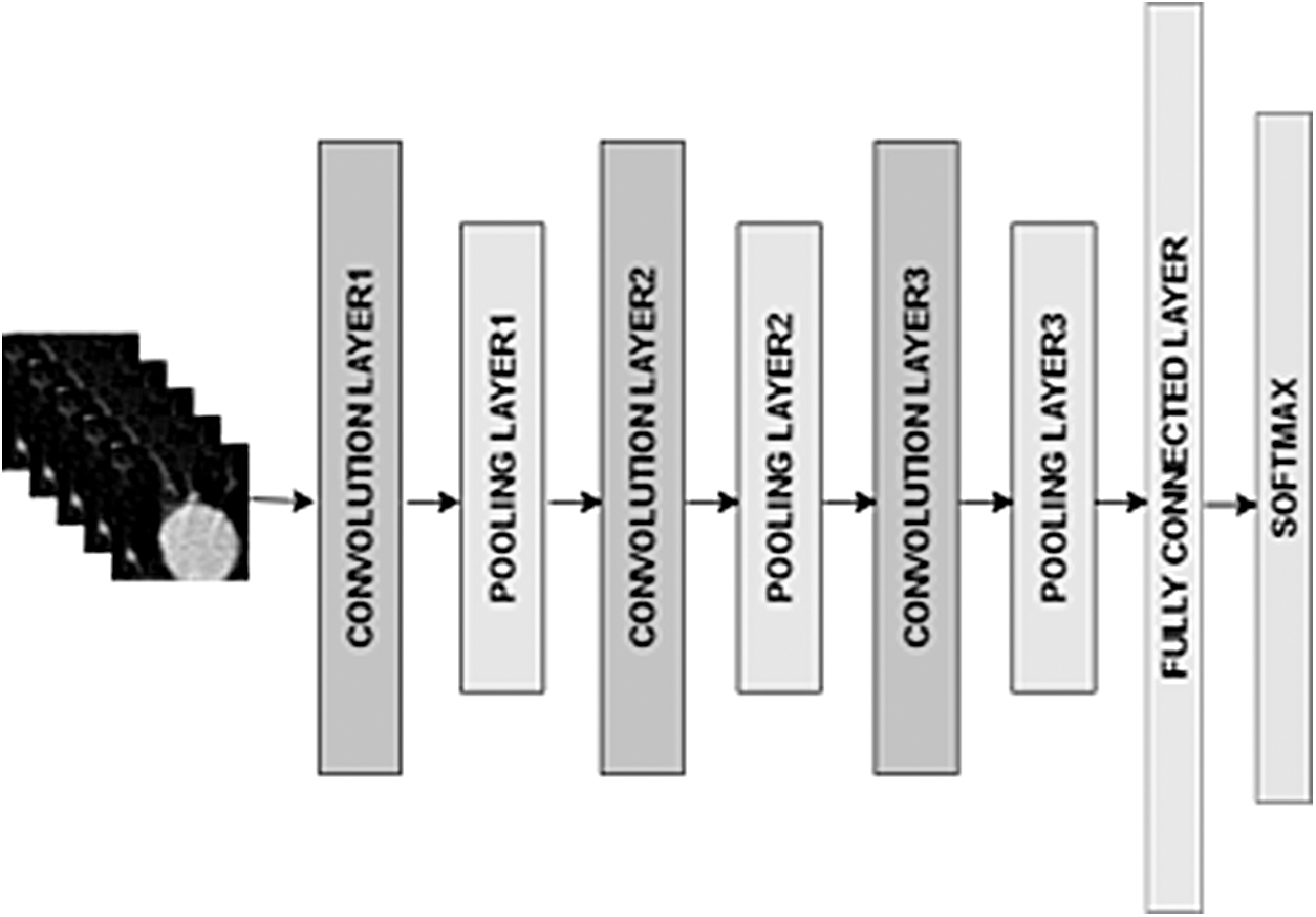
CNN architecture. CNN, convolution neural network.

Layer 1: The first convolution layer takes a nodule of size 50 × 50 as input. The size of the kernel in this layer is 3 × 3 with a stride of 1. This layer produces an output of 32 features of size 48 × 48. The output is then sent to the ReLu layer so that it can only retain the non-negative values. The output of the ReLU layer is sent to the max pooling layer of size 2 × to get 32 features of size 24 × 24.

Layer 2: The output of first max pool layer is fed to the second convolution layer. The second convolution layer uses a kernel of size 3 × 3 and a stride of 1 and generates 64 features of size 22 × 22. The output of convolution layer is sent to the ReLU layer, which is then followed by the max-pooling layer so as to reduce the dimensionality of image. The output of this layer is 64 features of size 11 × 11.

Layer 3: The output of second max pool layer is fed to the third convolution layer with a kernel of size 3 × 3 and a stride of 1. The output of the third convolution layer is 128 features of size 9 × 9 and is fed to the ReLU layer. The output is then fed to the max pooling layer to get 128 features of size 4 × 4.

Layer 4: The output of third max pooling layers is then flattened into a single vector and fed to a fully connected layer, which is a feed-forward neural network. This generates a vector of size 128.

Layer 5: The softmax classification layer is the final layer that converts the 128-feature map from the previous layer into two classes indicating the nodule as either malignant or benign.

Fractal features

Texture is a very important feature for analyzing images. Fractal was introduced by Mandelbrot in 1982 and is self-similar but may be irregular. Fractal dimension (FD) is one way of analyzing texture that gathers information about geometrical structure of fractal and measures the roughness and irregularity in image.¹⁶ FD is given by the following relationship: $F D = \frac{log N_{r}}{log \frac{1}{r}}$ (1)

Where $N_{r}$ is the number of self-similar components obtained after decomposing the images and r is the magnifying factor.

Several researchers have developed various techniques of finding the FD of image. Hartley and colleagues generated FD using the e-blanket method to analyze texture.¹⁷ FD was also generated by Pentland using Fourier power spectral density.¹⁸ Box counting methods were developed by Gangepain and Carmes in 1986. Several researchers have come with different variations in box-counting algorithm due to its weakness for certain image types. Chaudhuri and Sarkar used the differential box counting method to find FD of image.^19,20 Segmentation-based fractal texture analysis (SFTA)²¹ can also be used to determine the FD and has provided better accuracy and precision in image classification.

SFTA divides the input image into a set of binary images and the FDs are extracted from each of these regions.²² This task is accomplished using a two-threshold binary decomposition method. In this method, a list of threshold is calculated for each region using the multilevel Otsu algorithm. The Otsu threshold algorithm is recursively applied to each region until the predefined number of thresholds n_t is obtained. The grayscale image is divided into a set of binary images by picking a pair of thresholds and applying two-threshold segmentation algorithms as shown below: $B I (x, y) = \{\begin{matrix} 1 i f t_{l} < I (x, y) \leq t_{u} \\ 0, o t h e r w i s e \end{matrix}$ (2)

Where I(x,y) and BI(x,y) are grayscale and binary images, respectively, and $t_{l}$ and $t_{u}$ are lower and upper threshold values.

The next step is to calculate the border image denoted by B(x,y) and is computed as shown below: $B (x, y) = \{\begin{matrix} 1, i f \exists (x, y) N_{8} [(x, y)] : \\ B I (x, y) = 0 \hat{} B I (x, y) = 1 \\ 0, o t h e r w i s e \end{matrix}$ (3)

where $N_{8} [(x, y)]$ , the eight connected neighbor of the pixel BI(x,y).

The SFTA features are then extracted from the border image. SFTA features include pixel count (P) in each border image, mean gray values (M), and the FD (D). The FD is calculated from each border image using the Box counting method. In the Box counting method, the image is divided into grids of size s*s. And the grids containing at least one pixel of object are counted and denoted as N(s). The value of s is varied and a graph is plotted with log (N(s)) v/s log(s⁻¹). The curve obtained from the graph is approximated to a straight line and the FD (D) is determined by the slope of this line.

Gray-level co-occurrence matrix

Texture is a very important feature for analyzing images. Initially a co-occurrence matrix is created in four different directions of Ө, and with a specific distance “d” to determine the relative position of a pair of pixels in the respective direction. We then extract the statistical feature of texture using GLCM obtained from the lung nodule in CT scans. In this article, we considered the value of d = 1, 2, 3, 4 and Ө = 0°, 45°, 90°, 135° and hence creating 16 different gray-level co-occurrence matrices. Haralick et al.²³ used these co-occurrence matrices to define 14 statistical features. We extracted six texture features such as contrast, dissimilarity, homogeneity, angular second moment (ASM), energy, and correlation from four different co-occurrence matrices. The formulas for each of these features are given in Table 1.

Table 1.

Haralick features

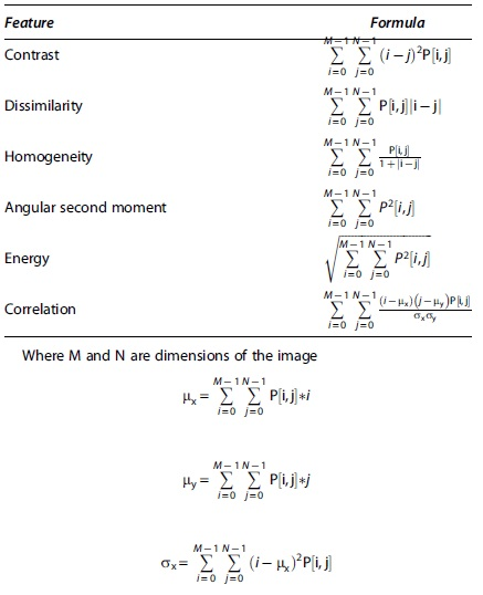
Since there are 16 co-occurrence matrices and six features defined for each co-occurrence matrix, 96 features are gathered from each image.

Support vector machine

SVM is a supervised learning algorithm developed by <QA>Cortes and Vapnik,²⁴ mostly used for binary classification that determines the hyperplane separating the two classes. SVM works well on high-dimensional data. It can also reduce the overfitting problem if the distance between the decision boundaries of hyperplanes is maximum also termed as maximum margin hyperplane or linear SVM. Linear SVM is mostly used for linear classification of data. For nonlinear classification, kernels can also be used to learn nonlinear decision boundary. We need to define the hyperplane such that $w_{t} ∙ x_{i} {+ b}^{3} + 1 w h e n y_{i} = + 1$ (4)

w_{t} ∙ x_{i} + b \leq - 1 w h e n y_{i} = - 1

(5)

Where x_i is a set of features, w_t is a set of weights, b is bias, and y_i is the predicted output value. The problem can be optimized by increasing the margin between hyperplanes as shown below:

Such that $w^{T} x_{n} t_{n}$ ≥ 1− $ξ_{n}$ , $ξ_{n} \geq 0$ , n = 1,2,3.…N

Where $ξ_{n}$ is slack variable and t_n ∈ {+1,−1}

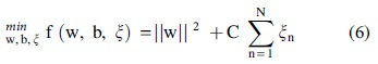
Softmax is the last layer in most of the deep learning models used for classification. The last layer of deep learning model can be replaced by SVM. We use linear SVM with L2 loss to minimize the squared hinge loss as shown in Equation (7).

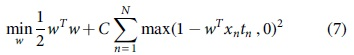
L2 penalty can also reduce the overfitting problem.

Proposed Model

Architecture

In this article, we propose to design and implement a model combining the features extracted from deep learning model with statistical texture features and finally classify the features using SVM. The CNN model has shown better accuracy in lung nodule classification. There are several CNN architectures such as AlexNet, LeNet, ResNet, DenseNet, VGG, and Inception. However, ResNet and DenseNet have shown promising results with respect to lung nodule classification. Hence, we extract the features from a deep learning model such as CNN (with three layers), ResNet, and DenseNet to evaluate the proposed approach. We gathered two key texture features: Haralick features and fractal features for analysis. Haralick features are calculated from the gray-level co-occurrence matrices by calculating the number of occurrences of gray levels for a given distance and angle. Fractal features are obtained by decomposing the grayscale image into a predefined set of binary images and then extracting mean, total number of pixels, and FD for each binary image.

The proposed work was evaluated on the LUNA data set, which has CT images stored in metaimage format and an annotation file containing information about UID, x, y, z coordinates of each finding, and the class it belongs to. Nodules were cropped based on the Cartesian coordinates mentioned in the annotation file to retrieve the annotations. However, there is a huge imbalance in benign and malignant nodules. Hence, we use data augmentation and downsampling methods to reduce the imbalance in data sets. Data augmentation was achieved by rotating the image by 90° and 180°.

A brief explanation of the proposed architecture is demonstrated in Figure 2.

FIG. 2.

Proposed architecture. GLCM, gray-level co-occurrence matrix; PCA, principal component analysis; SVM, support vector machine.

The input given to the model is a segmented grayscale image of the lung nodule. The nodule was segmented based on the region of interest mentioned in the candidate file provided by LUNA data set, which is named as annotation.csv. The size of each segmented lung nodule is 50 × 50. We extract three different features from the segmented lung nodule simultaneously, that is, CNN features, GLCM features, and fractal features. The image is passed through three layers of CNN model, where each layer consists of convolution and pooling layer. The output of feature extraction phase of the CNN model is fed to a fully connected layer to get a final set of CNN features. Before the feature is extracted from the image, we also train the CNN model with training data sets so as to update the weights. The lung nodule is also converted into 16 gray-level co-occurrence matrices for different values of theta and displacement to extract 96 Haralick features. Apart from the Haralick texture feature, we also extract fractal features using the two-threshold binary decomposition and by applying the SFTA feature extraction algorithm. CNN features are combined with the Haralick and fractal features and fed to the SVM classifier to predict the malignancy of the nodule. SVM has proven to be a very good two-group classifier with a high-dimensional feature map.¹⁹ Before applying the SVM classifier, the dimensionality of the features can be reduced by the principal component analysis (PCA) technique so as to retain the information gathered from the combined feature map.

Data set is divided into training and testing sets. Before extracting the CNN features from the CNN model, we train the model using 1534 images. The trained model is then used for feature extraction. A brief discussion of the training and testing process is shown in the Figure 3. In the training phase, the CNN, fractal, and GLCM features are extracted from the training set and are concatenated. The dimensionality of these feature sets is reduced using the PCA technique to reduce the computation time, and finally, these selected features are used in training the SVM model with L2 regularization. We used 10-fold cross-validation to evaluate the classification model. In the testing phase, the CNN, fractal, and GLCM features extracted from the test data set are concatenated and reduced using the PCA technique. The final features are then used to predict the malignancy of the model using trained linear SVM classifier.

FIG. 3.

Training and testing process of proposed work.

Algorithm 1 shows feature extraction and classification stage in the training process.

Algorithm 1. Training Process in Proposed Work
Input: Training samples
Output: Classification Result with model performance
1. Initialize the number of epochs and batch size
2. Train the CNN architecture with an explicit training set
3. for each image in training set do
F1← Extract the Deep features using trained CNN architecture
end for
4. for each image in training set do
F2← Extract GLCM features like contrast, dissimilarity, homogeneity, ASM, energy and correlation.
end for
5. for each image in training set do
Apply two threshold binary decomposition
F3←Extract fractal features using SFTA algorithm
end for
6. Final features ← F1 + F2 + F3
7. Train SVM model with the final features extracted from the train set

DenseNet architecture

Although the CNN model has shown accurate results, it has been observed that the accuracy and efficiency of the model can be increased if there exists a shorter connection between input and output by concatenating the output of previous layers with the current layers. Hence, Huang et al. introduced the Dense convolutional network that connects each layer with every other layer in the network so as to restore the information that may get vanished as the features gets propagated through a larger path.

An explanation of DenseNet architecture is shown in Figure 4. DenseNet architecture consists of dense blocks and each dense block consists of densely connected layers. The input to the DenseNet model is cropped nodule. Each layer in the dense block takes input from the output of previous layers. Each dense layer consists of convolution and concatenation layers. Each convolution layer is made up of batch normalization, activation, and convolution unit. Multiple dense blocks are separated from each other by a transition layer so that each layer maintains a feature map of same size in every dense block. Each transition layer consists of batch normalization, activation, convolution, and average pooling layer. Since CNN provides better accuracy and efficiency with DenseNet architecture, we used the DenseNet model to extract the deep features.

FIG. 4.

DenseNet architecture with three dense blocks.

ResNet architecture

As the number of layers in a network increases beyond a particular threshold, the accuracy of the network reduces due to vanishing gradient problem. The ResNet model tried solving this issue by skipping training of few layers and thus creating a residual block. In our study, we used ResNet-20, ResNet-56, and ResNet-164, which use 3, 9, and 27 residual blocks, respectively. Each residual block consists of convolution, batch normalization, and activation. A brief description of ResNet model is shown in Figure 5. The segmented lung nodule is fed to the convolutional layer utilizing convolution of size 1 × 1, which is then followed by a series of residual block. At the start of each stage, the number of feature maps is halved, but the number of filters is doubled. Finally, the dimensionality of the feature set is reduced using average pooling.

FIG. 5.

ResNet architecture with 20 layers.

Advantages and disadvantages

In the proposed work, we achieve high performance due to two novel approaches. First, it uses a combination of texture and deep features to collectively gather the benefits of extracting high-level features of image, using deep network and spatial variation of pixel. GLCM features can easily differentiate benign and cancerous nodules in CT images with an accuracy of 90.3%.^25,26 By adding fractal feature to GLCM features, the sensitivity of classification system increases. Also, the use of feature selection algorithm helps in selecting the most relevant features from all three methods, thus gathering the strengths of each method. Second, we use the SVM classifier instead of softmax classifier to provide a slight improvement in the accuracy of classification system.

Our method works poorly on ground glass opacity (GGO) nodules as there are limited GGO images in the LUNA data set, which is being used in our study. Also, the GLCM method is also computationally expensive. A brief idea of the features extracted in the proposed work is demonstrated in Figure 6.

FIG. 6.

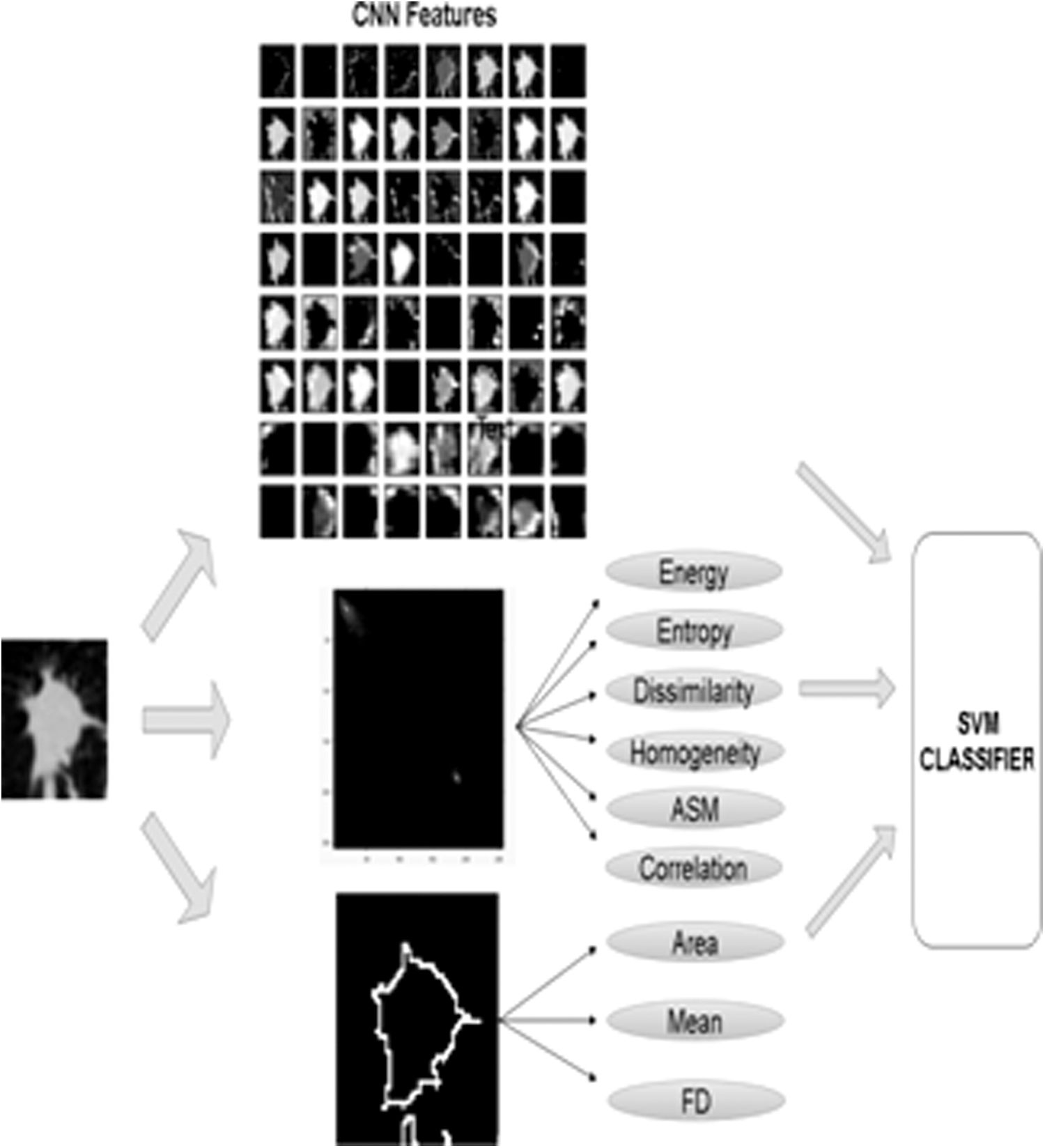
Features extracted in proposed work. ASM, angular second moment; FD, fractal dimension.

Results and Experiments

Experimental setup

The data set was evaluated with i7 processor, NVIDIA GeForce RTX 2070 (8GB on-board memory). The implementation of our networks is based on keras 2.2.4 library with tensor flow as backend.

Data description

To evaluate the model, we conducted the experiments on data from the publicly available data set LUng Nodule Analysis 2016 (LUNA16),¹⁸ containing 888 CT scan images collected from LIDC-IDRI. The scans of each individual contain 200 slices, each of size 512 × 512 pixels. A team of four radiologists have evaluated these nodules and if the average score of the four radiologists is more than 3, the nodule is considered malignant or else it is flagged as benign. The data set uses 551,065 annotations, out of which, 1351 were labeled as malignant and the rest are benign. To reduce this imbalance in the data set, we use data augmentation and downsampling methods for false-positive reduction. In the downsampling method, we reduce the number of negative samples in the ratio of 10:1 (10 negative and 1 positive sample), thus selecting 5515 images with negative labels. We also increase the number of positive samples by augmenting the images (i.e., rotating the images by 90° and 180°) and thus generating 4053 images with positive labels.

Simulation

The LUNA data set also maintains a annotation file, which keeps record of the x, y, z coordinates of the nodule. Nodules were then cropped based on the coordinates mentioned in the annotation file provided by the LUNA data set. The database consists of 9568 images. Six thousand one hundred thirty-one images are used for training, and 1903 images are used for testing. Remaining 1534 images are used to train the CNN model. After pretraining the model with 1534 images, deep features are extracted from the trained model in the proposed work, during the training and testing phases, respectively. To evaluate the proposed approach, we used three CNN architectures: CNN with three convolution layers, ResNet, and DenseNet. We used 1534 images to train the network before extracting the features.

A transfer learning model could also be used to extract the deep features. However, in the proposed approach, we trained the model from scratch with 1534 train data sets instead of using a transfer learning approach due to change in modality of data sets. As the natural images differ from medical images such as CT,²⁷ we prefer to train the deep models from scratch.

We train the CNN (three layers) with the learning rate and batch size of 0.02 and 100, respectively. The number of epochs used in training for all three networks was 70. The loss function in CNN training was categorical cross-entropy. In this experiment, the Adam optimizer provided a better training performance. After every epoch, the weights were updated. To train a DenseNet model, we used three dense blocks. Each dense block contains 12 dense layers. The growth rate or number of filters for each dense block was 12. The dropout rate used after each convolution layer is 0.2. We trained a ResNet model with a learning rate of 0.001. There are three stages in ResNet and each stage has residual blocks. The number of residual blocks in ResNet-20, ResNet-56, and ResNet-164 is 3, 9, and 27, respectively. In each stage, the residual block learns the same number of filters. The trained deep learning model is used to generate the deep feature map for training and testing data. Segmented lung nodule is the input to the model.

To extract the Haralick features, we convert the grayscale image into 16 GLCM for a displacement d = 1, 2, 3, and 4 and angle Ө = 0°, 45°, 90°, 135°. We extract six statistical features such as contrast, dissimilarity, homogeneity, ASM, energy, and correlation from each of these matrices. Thus, the resulting number of Haralick feature is 96. Fractal features are extracted by performing two basic steps. Two-threshold binary decomposition and SFTA feature extraction. In the two-threshold binary decomposition phase, Otsu's algorithm is applied recursively until we obtain the desired number of threshold (n_t). The value of n_t is set to 4 and the total number of binary images obtained by the two-threshold segmentation algorithm is 2*n_t = 8. In SFTA feature extraction phase, we extract three features: total number of pixels (P), mean gray values (M), and the FD from each of the binary image. Hence, the resulting number of fractal features is n_t*3.

In the training phase, all the features extracted from the deep learning model are concatenated with fractal and GLCM features. Since GLCM features have a higher value when compared with the deep features, we normalize the concatenated features. The numbers of concatenated features are comparatively huge, and hence, the accuracy of the model could decrease due to the increase in features or dimension. Hence, we use PCA to reduce the feature dimension. We fit PCA on training data and apply the transform on train and test data to reduce the dimensionality of feature sets of train and test data set, respectively. We choose minimum number of principal components by retaining 95% of variance. The final feature obtained from the PCA technique is used to train the linear SVM with L2 loss function.

In the testing phase, we use the trained deep learning model to extract the deep features from the test set and concatenate it with its fractal and GLCM features. We use the trained parameters of PCA obtained from the training phase and apply them to calculate PCA on test set. The feature set thus selected is then used to classify the lung nodules into cancerous and noncancerous type using trained SVM classifier. We classified the extracted feature set with several classifiers such as SVM, decision tree, linear regression, naive Bayes, K-nearest neighbor (with two neighbors), and AdaBoost. The AdaBoost classifier was built using a leaning rate of 0.1 and the number of estimator was 50 using decision trees as our base estimator. Our experimental results showed that the accuracy of SVM classifier was found to provide a better accuracy of 92.85% when compared with other classifiers, as shown in Table 2.

Table 2.

Accuracy of proposed work with different classifiers on convolution neural network model

Classifier	Accuracy (%)	Precision (%)	Recall (%)
SVM	92.85	84.53	91.29
Decision tree	91.32	83.27	88.45
Linear regression	91.69	82.82	90.76
Naive Bayes	90.22	80.35	88.63
K-nearest neighbor	90.90	88.69	79.39
AdaBoost	91.09	81.51	90.05

SVM, support vector machine.

SVM works better on unstructured high-dimensional data sets such as images and also prevents the overfitting problem. Hence, the model is trained using L2-SVM objective function.

Figure 7 shows the learning curve of SVM classifier, which shows the validation and training score of estimator for different training samples. We see that the training score is around maximum and the validation score increases with more training samples. The training score of SVM is greater than the validation score and adding more training data increases generalization.

FIG. 7.

Learning curve of SVM classifier.

Figure 8 shows a plot of training and validation score of SVM classifier for different values of gamma parameter.

FIG. 8.

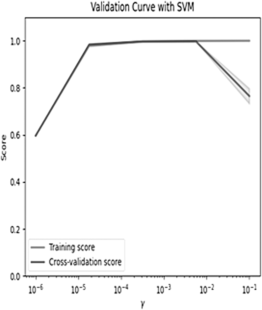
Validation curve of SVM classifier.

In Figure 8, we observe that for low value of gamma, the training and validation score is as low as 0.58, indicating that the model does not predict well for new data as well as training data. However, for a higher value of gamma, the training score is high, but the validation score is low indicating that the model does not work well on unseen data. We performed 10-fold cross-validation on the training set, that is, training set was divided into 10 folds where the training and testing data set was changed in each iteration. Our model attains a mean R-squared value of 0.996 for 10-fold cross-validation.

We evaluated the accuracy of the CNN model in addition to statistical features such as GLCM and fractal and observed that the accuracy of proposed work showed significant improvement of 92.85% with addition of texture features, when compared with using CNN features alone, as shown in Figure 9.

FIG. 9.

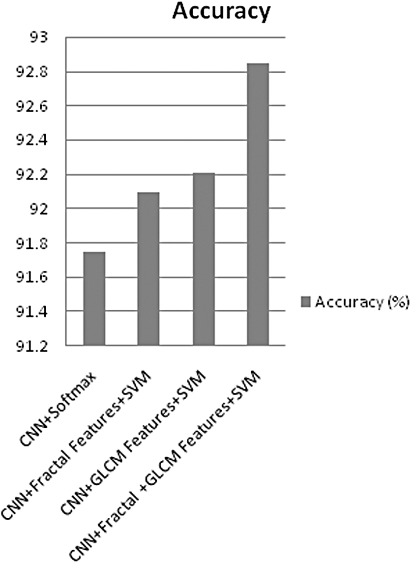
Accuracy with different combinations of feature and classifier.

CT texture analysis provides significant information about tumor characteristics. The intensity of the pixel in a CT image determines the physical characteristics of lung. Gathering these characteristics using texture analysis can help differentiate the cancerous cells from normal cells. GLCM features give comparatively better results than fractal features when combined with deep features. The FD of malignant nodules was higher when compared with benign nodules. Although fractal features are extensively used in classifying biomedical images, FD may not be sufficient to distinguish all textures, as an object having different appearances can have same FDs. We classified the nodules using (1) GLCM features, (2) fractal features, and (3) a combination of GLCM and fractal features, as shown in Figure 10.

FIG. 10.

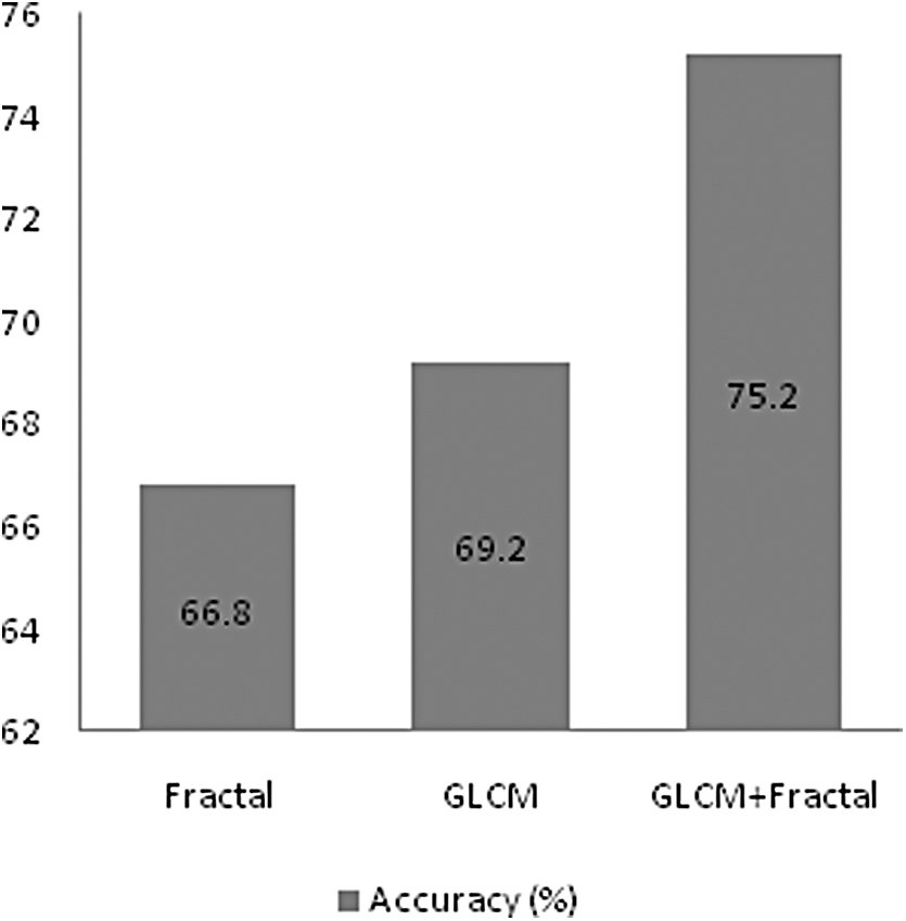
Accuracy with different features using SVM classifier.

It is evident from Figure 10 that the accuracy of classification system is better with GLCM features when compared with fractal features. However, the combination of both GLCM and fractal features has improved the accuracy of the classification system. GLCM and fractal features appear to have their own strengths and weaknesses, but the combination of both with deep features has shown significant improvement in accuracy.

For the classification problem, feature selection plays an important role in selecting the most relevant subset of features by removing redundant and irrelevant features. In the proposed work, we used PCA to select the relevant features from the feature list. We also compared PCA with other feature selection algorithms such as Lasso with L2 regularization. The feature vector was classified using SVM classifier and the testing accuracy was noted. Figure 11 shows comparison of testing accuracy of proposed model with (1) PCA dimensionality reduction technique, (2) Lasso feature selection technique, and (3) without using any feature selection method.

FIG. 11.

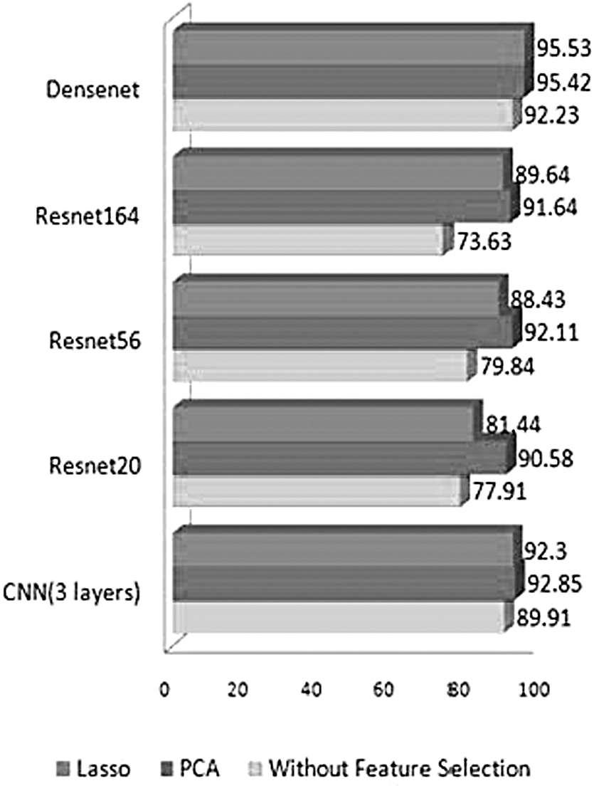
Comparison of accuracy of proposed approach with and without the feature selection technique.

It is evident from Figure 11 that the classifier shows better performance when the dimensionality of the features is reduced. Feature selection phase not only reduces the dimension of input features but also improves the performance of classification system as it reduces the redundant features. PCA and Lasso have shown equivalent results, with the accuracy of PCA being marginally better than Lasso.

We also validated the proposed approach with different deep learning models and have noted an increase in accuracy with the use of proposed model. Figure 12 shows comparison of accuracy of different learning models using slight variation in feature extraction and classification, from which it is evident that the accuracy of the deep learning models increases with the addition of fractal and GLCM features and then classifying them using SVM classifier.

FIG. 12.

Comparison of accuracy of proposed approach with different deep learning models.

We observe that the DenseNet architecture has shown better accuracy when compared with other CNN architectures such as AlexNet, ResNet20, ResNet56, ResNet164 with both SVM and softmax classifiers. This is because DenseNet concatenates feature maps from different layers, thus increasing the variation in input in each layer and improving efficiency.

Receiver operating characteristic (ROC) curve and area under curve (AUC) help in determining the performance of the classification. The AUC score of the model is 0.95, which indicates that the model has shown good measure of separation between positive and negative classes. The ROC curve is a graph of true-positive rate versus false-positive rate at different thresholds, which is shown in Figure 13.

FIG. 13.

ROC curve of proposed work with DenseNet architecture. AUC, area under curve; ROC, receiver operating characteristic.

The free-response ROC curve of our proposed work is shown in Figure 14. The average sensitivity (competition performance metric) of lung nodule detection is 0.875 at seven different false-positive rates: 1/8, 1/4, 1/2, 1, 2, 4, and 8 false positives per scan.

FIG. 14.

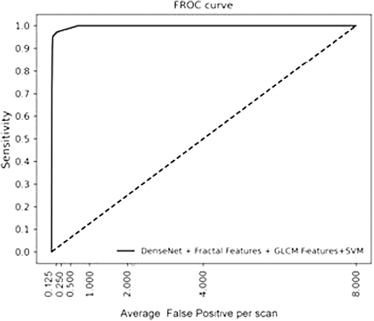
FROC curve of proposed work with DenseNet architecture. FROC, free-response receiver operating characteristic.

Some of the nodules that were detected by the proposed model are visually represented in Figure 15. The proposed model could detect nodules of different sizes, locations, and margins.

FIG. 15.

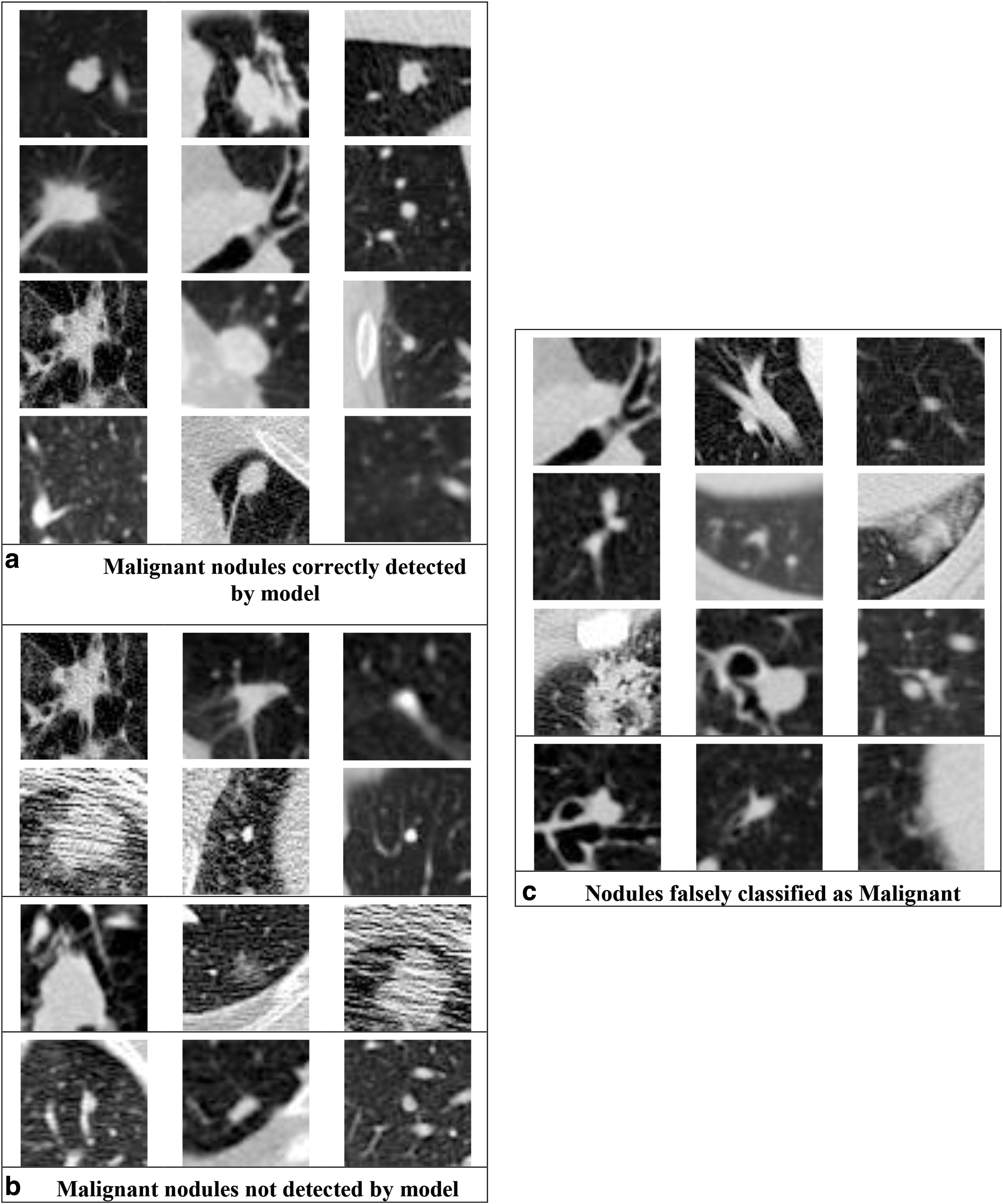
Visual representation of nodules detected and not detected using proposed approach. (a) Malignant nodules correctly detected by model. (b) Malignant nodules not detected by model. (c) Nodules falsely classified as malignant.

To evaluate the correctness of our classifier, we use these four metrics: accuracy, sensitivity, specificity, and positive predictive value.

The formulas for each of these metrics are given below for reference: $A c c u r a c y = \frac{T P + T N}{T P + T N + F P + F N}$ $S e n s i t i v i t y = \frac{T P}{T P + F N}$

S p e c i f i c i t y = \frac{T N}{T N + F P}

P o s i t i v e P r e d i c t i v e V a l u e = \frac{T P}{T P + F P}

Where TP, TN, FP, and FN are true positive, true negative, false positive, and false negative, respectively, obtained from the confusion matrix.

Table 3 gives a summary of accuracy of the proposed approach in concatenation with different deep learning features.

Table 3.

Accuracy of different deep learning models without proposed approach

Proposed work with different deep learning models	Accuracy(%)	Sensitivity(%)	Specificity (%)	Positive predictive value (%)
CNN features²⁸ +Fractal +GLCM +SVM	92.85	96.37	84.98	93.20
ResNet20²⁹ +Fractal +GLCM +SVM	90.58	95.27	77.90	91.78
ResNet56²⁹ +Fractal +GLCM +SVM	90.94	85.01	67.74	87.30
ResNet164²⁹ +Fractal +GLCM +SVM	91.64	92.76	77.90	95.03
DenseNet³⁰ +Fractal +GLCM +SVM	95.42	97.49	93.97	95.96

CNN, convolution neural network; GLCM, gray-level co-occurrence matrix.

From Table 3, it is evident that the proposed work has shown best results with features extracted from the DenseNet model, with a classification accuracy of 95.42%. The proposed work is quite reliable as the sensitivity is high with a value of 97.49%, thus reducing the risk of missed diagnosis.

Figure 16 gives a comparison of ROC curve with respect to other deep learning models using the proposed approach. It is evident from the figure that DenseNet architecture with the proposed approach has shown excellent performance with respect to lung nodule classification.

FIG. 16.

Comparison of ROC curve of proposed approach with different deep learning models.

It is worth noting that, in Figure 17, the proposed approach with DenseNet architecture has achieved the best performance compared with other models with less false positives per scan.

FIG. 17.

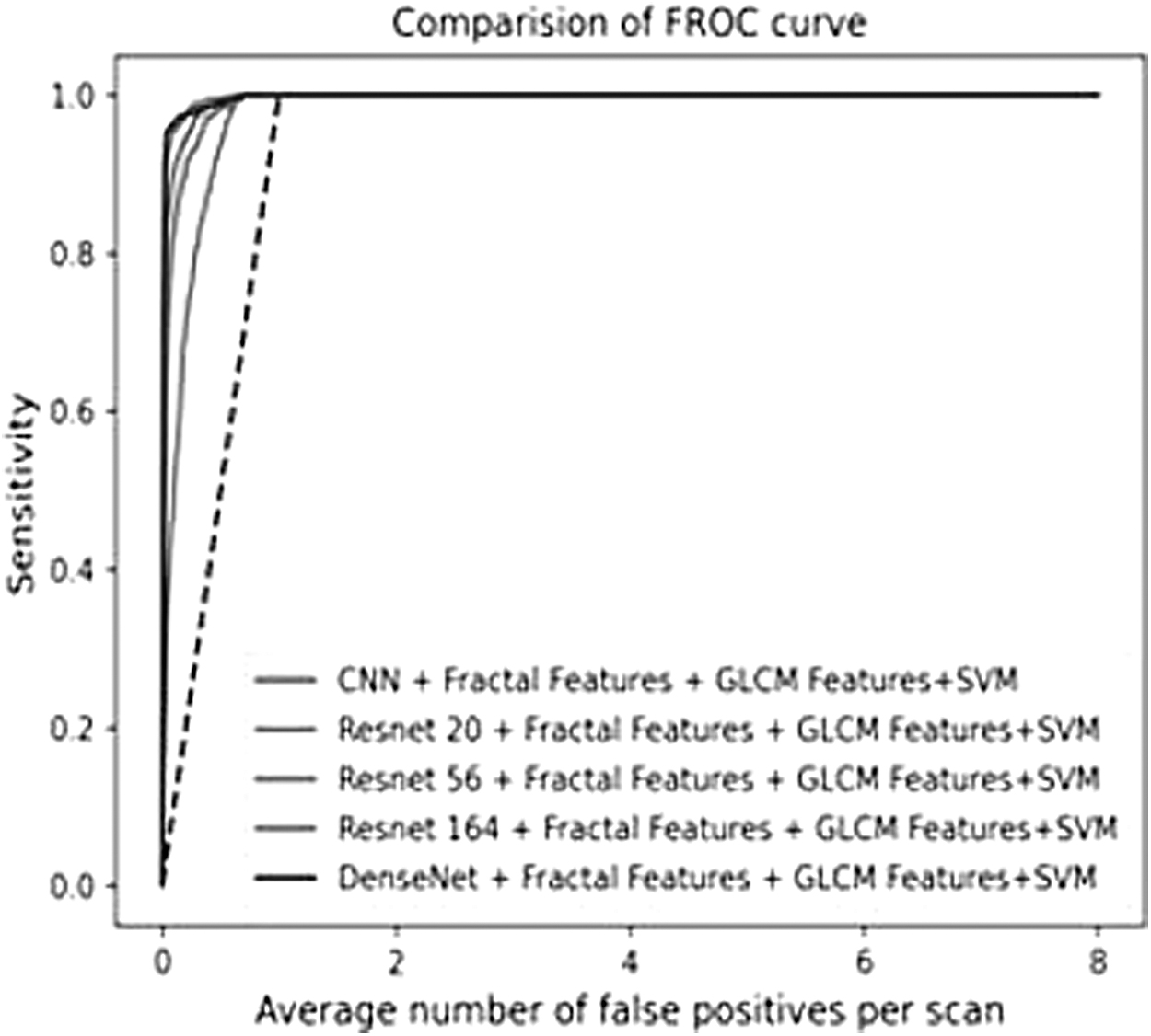
Comparison of FROC curve of proposed approach with different deep learning models.

The sensitivity of the proposed work was compared with other state-of-the-art works in literature, using the LUNA data set, shown in Figure 18.

FIG. 18.

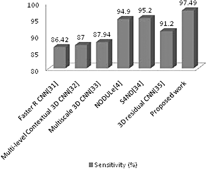
Comparison of the proposed work with other CNN architectures using the LUNA16 data set. LUNA16, LUng Nodule Analysis 2016; S4ND, single-shot single-scale lung nodule detection.

Our method shows better sensitivity when compared with other works mentioned in literature using the same data set, as shown in Figure 18.

Conclusion

In this article, a computer-aided detection system was proposed using CNN, fractal, and GLCM features of lung nodules and the SVM classifier to detect the malignancy of the pulmonary nodule. Our results showed that the combination of texture features such as fractal and GLCM with CNN improves the accuracy of the system, when classified using the SVM classifier. The proposed system has provided an accuracy of 95.42%, sensitivity of 97.49%, and specificity of 93.97%, and a positive predictive value of 95.96% when texture features were combined with deep features extracted from the DenseNet architecture. However, the accuracy can still be improved by preprocessing the image removing noise. We also observed that SVM classifier has provided better classification accuracy when compared with other classification algorithms. It was observed that the accuracy of classification system increases with the addition of new texture features.

Footnotes

Author Disclosure Statement

No competing financial interests exist.

Funding Information

This research did not receive any specific grant from funding agencies in the public, commercial, or not-for-profit sectors.

Abbreviations Used

References

Bray

, Ferlay

, Soerjomataram

, et al. Global cancer statistics 2018: GLOBOCAN estimates of incidence and mortality worldwide for 36 cancers in 185 countries. CA Cancer J Clin. 2018; 68:394–424.

Yamashita

, Nishio

, Do

RKG

. et al. Convolutional neural networks: An overview and application in radiology. Insights Imaging. 2018; 9:611–629.

Silva

GLF

, Valente

TLA

, Silva

, et al. Convolutional neural network-based PSO for lung nodule false positive reduction on CT images. Comput Methods Programs Biomed. 2018; 162:109–118.

Zhan

, Xia

, Zeng

, et al. NODULe: Combining constrained multi-scale LoG filters with densely dilated 3D deep convolutional neural network for pulmonary nodule detection. Neurocomputing. 2018; 317:159–167.

Chen

, Qin

, Ji

, et al. Automatic scoring of multiple semantic attributes with multi-task feature leverage: A study on pulmonary nodules in CT images. IEEE Trans Med Imaging. 2017; 36:802–814.

Setio

AAA

, Ciompi

, Litjens

, et al. Pulmonary nodule detection in CT images: False positive reduction using multi-view convolutional networks. IEEE Trans Med Imaging. 2016; 35:1160–1169.

Tafti

, Bashiri

, LaRose

, et al. Diagnostic classification of lung CT images using deep 3D multi-scale convolutional neural network. In: 2018 IEEE International Conference on Healthcare Informatics (ICHI), New York, NY: IEEE, 2018. pp. 412–414.

Kumar

, Mukhopadhyay

, Khandelwal

3D texture analysis of solitary pulmonary nodules using co-occurrence matrix from volumetric lung CT images. In: Proceedings of the SPIE Medical Imaging Conference, WA: SPIE, 2013. pp. 1–4.

Wang

, Wu

, Sun

, et al. Prediction models for solitary pulmonary nodules based on curvelet textural features and clinical parameters. Asian Pac J Cancer Prev. 2013; 14:6019–6023.

10.

Wang

, Wu

, Sun

, et al. Combination of radiological and gray level co-occurrence matrix textural features used to distinguish solitary pulmonary nodules by computed tomography. J Digit Imaging. 2013; 26:797–802.

11.

Alalshekmubarak

, Smith

. A novel approach combining recurrent neural network and support vector machines for time series classification. In: 9th International Conference on Innovations in Information Technology (IIT), Abu Dhabi, UAE: IEEE, 2013. pp. 42–47.

12.

Szarvas

, Yoshizawa

, Yamamoto

, et al. Pedestrian detection with convolutional neural networks. In: Proceedings of the IEEE on Intelligent Vehicles Symposium, Las Vegas, USA: IEEE, June 2005. pp. 224–229.

13.

Niu

X-X

, Suen

. A novel hybrid CNN–SVM classifier for recognizing handwritten digits. Pattern Recognit. 2012; 45:1318–1325.

14.

, Huang

, Wang

, et al. A CNN-SVM combined model for pattern recognition of knee motion using mechanomyography signals. J Electromyogr Kinesiol. 2018; 42:136–142.

15.

Tang

Deep learning using linear support vector machines. Workshop on Challenges in Representation Learning. ICML. 2013; arXiv preprint arXiv:1306.0239.

16.

Biswas

, Ghose

, Guha

, et al. Fractal dimension estimation for texture images: A parallel approach. Pattern Recognit Lett. 1993; 19:309–313.

17.

Peleg

, Naor

, Hartley

, et al. Multiple resolution texture analysis and classification. IEEE Trans Pattern Anal Mach Intell. 1984; PAMI-6:518–523.

18.

Pentland

AP.

Shading into texture. Artif Intell. 1986; 29:147–170.

19.

Chaudhuri

, Sarkar

. Texture segmentation using fractal dimension. IEEE Trans Pattern Anal Mach Intell. 1995; 17:72–77.

20.

Sarkar

, Chaudhuri

. An efficient differential box-counting approach to compute fractal dimension of image. IEEE Trans Syst Man Cybern. 1994; 24:115–120.

21.

Costa

, Humpire-Mamani

, Traina

AJM

. An efficient algorithm for fractal analysis of textures. In: 25th SIBGRAPI Conference on Graphics, Patterns, and Images (SIBGRAPI), Ouro Preto, Brazil: IEEE, 2012. pp. 39–46.

22.

Costa

, Tekli

, Traina

AJM

. Fast fractal stack: fractal analysis of computed tomography scans of the lung. In: Proceedings of the 2011 International ACM Workshop on Medical Multimedia Analysis and Retrieval (MMAR ’11), New York, NY: Association for Computing Machinery, 2011. pp. 13–18.

23.

Haralick

, Shanmugam

, Dinstein

. Textural features for image classification. IEEE Trans Syst Man Cybern. 1973; SMC-3:610–621.

24.

Cortes

, Vapnik

. Support-vector networks. Mach Learn. 1995; 20:273–297.

25.

Petkovska

, Shah

, McNitt-Gray

, et al. Pulmonary nodule characterization: A comparison of conventional with quantitative and visual semi-quantitative analyses using contrast enhancement maps. Eur J Radiol. 2006; 59:244–252.

26.

McNitt-Gray

, Hart

, Wyckoff

, et al. A pattern classification approach to characterizing solitary pulmonary nodules imaged on high resolution CT: Preliminary results. Med Phys. 1999; 26:880–888.

27.

, Girshick

, Dollár

. Rethinking ImageNet pre-training. In: 2019 IEEE/CVF International Conference on Computer Vision (ICCV). Seoul, Korea: IEEE,, 2019; pp. 4917–4926. arXiv:1811.08883.

28.

Krizhevsky

, Sutskever

, Hinton

. 2017. ImageNet classification with deep convolutional neural networks. Commun ACM. 2017; 60:84–90.

29.

, Zhang

, Ren

, et al. Deep residual learning for image recognition. In: 2016 IEEE Conference on Computer Vision and Pattern Recognition (CVPR), Las Vegas, NV: IEEE, 2016. pp. 770–778.

30.

Huang

, Liu

, Van Der Maaten

, et al. Densely connected convolutional networks. In: 2017 IEEE Conference on Computer Vision and Pattern Recognition (CVPR), Honolulu, HI: IEEE, 2017. pp. 2261–2269.

31.

Xie

, Yang

, Sun

, et al. Automated pulmonary nodule detection in CT images using deep convolutional neural networks. Pattern Recognit. 2019; 85:109–119.

32.

Dou

, Chen

, Yu

, et al. Multilevel contextual 3-D CNNs for false positive reduction in pulmonary nodule detection. IEEE Trans Biomed Eng. 2017; 64:1558–1567.

33.

, Lu

, Yang

, et al. Automatic lung nodule detection using a 3D deep convolutional neural network combined with a multi-scale prediction strategy in chest CTs. Comput Biol Med. 2018; 103:220–231.

34.

Khosravan

, Bagci

. S4ND: Single-shot single-scale lung nodule detection. In: Frangi

, Schnabel

, Davatzikos

, (Eds.): Medical Image Computing and Computer Assisted Intervention – MICCAI 2018. MICCAI 2018. Lecture Notes in Computer Science, vol. 11071. Cham: Springer. pp. 794–802.

35.

Jin

, Li

, Tong

, et al. A deep 3D residual CNN for false-positive reduction in pulmonary nodule detection. Med Phys. 2018; 45:2097–2107.