A Long Short-Term Memory Network Stock Price Prediction with Leading Indicators

Abstract

The accuracy of the prediction of stock price fluctuations is crucial for investors, and it helps investors manage funds better when formulating trading strategies. Using forecasting tools to get a predicted value that is closer to the actual value from a given financial data set has always been a major goal of financial researchers and a problem. In recent years, people have paid particular attention to stocks, and gradually used various tools to predict stock prices. There is more than one factor that affects financial trends, and people need to consider it from all aspects, so research on stock price fluctuations has also become extremely difficult. This paper mainly studies the impact of leading indicators on the stock market. The framework used in this article is proposed based on long short-term memory (LSTM). In this study, leading indicators that affect stock market volatility are added, and the proposed framework is thus named as a stock tending prediction framework based on LSTM with leading indicators (LSTMLI). This study uses stock markets in the United States and Taiwan, respectively, with historical data, futures, and options as data sets to predict stock prices in these two markets. We measure the predictive performance of LSTMLI relative to other neural network models, and the impact of leading indicators on stock prices is studied. Besides, when using LSTMLI to predict the rise and fall of stock prices in the article, the conventional regression method is not used, but the classification method is used, which can give a qualitative output based on the data set. The experimental results show that the LSTMLI model using the classification method can effectively reduce the prediction error. Also, the data set with leading indicators is better than the prediction results of the single historical data using the LSTMLI model.

Introduction

The financial market is a mechanism for determining the price of financial funds and trading financial assets. It is a market that enables the financing of securities and the trading of securities. The capital market is also called the “long-term financial market,” mainly the stock market, fund market, and bond market. Its volatility can reflect the degree of risk of assets. The fluctuation of stock prices plays a considerable role in the appropriate timing of buying and selling stocks.¹

For investors, the true meaning of investing in the stock market is to obtain extraordinary returns by buying low and selling high, and so, the prediction of stock price fluctuations has become a particular focus of private investors and investment companies.² Due to a large amount of data in stocks, the low data correlation, and the many factors that affect stock prices, financial markets are full of uncertainty, making predicting stock price fluctuations a significant problem for stock researchers. Initially, people had predicted the fluctuations of stock prices several times,^3,4 but the results were unsatisfactory.

In the literature, research on the stock market has become more frequent. The efficient market hypothesis proposed⁵ in 1970 believed that the price of stocks could not be predicted. There is a questionable premise of the efficient market hypothesis; that is, all market investors have sufficient rationality to be able to quickly and accurately judge market information. However, investors are not completely rational. For example, people may have positive or negative emotions at certain moments.^6–9 Therefore, after this hypothesis was raised, there were both support and opposition, thus becoming one of the most controversial investment theories.^10,11 Some researchers believe that if the trading signals¹² of the stocks can be found, the stocks can be bought and sold at the appropriate time to obtain relatively high profits. With the emergence of powerful machine learning algorithms, the efficient market hypothesis has caused heated discussions among market investors. The support vector machine (SVM) is a binary classification model. Although it has not appeared for a long time, it has good classification performance in the field of machine learning. Huang et al.¹³ found in 2005 that SVMs have better prediction results than traditional statistical methods. Nayak et al.¹⁴ proposed a hybrid model for the prediction of Indian stock indexes. This model mainly uses two machine learning algorithms, namely SVM and k-nearest neighbor. Studies have shown that the hybrid model they proposed has good scalability and predictability for high-dimensional data.

Although the prediction results of SVM are significantly improved compared with other models,^15,16 it is still not satisfactory for stock prediction. Neural networks, evolutionary computation,¹⁷ and fuzzy logic composed of intelligent computing. The neural network model has received particular attention. Because neural network models can identify nonlinear relationships in data sets, many researchers have analyzed and predicted stock price fluctuations based on various neural networks and have also obtained relatively good results. For the Tokyo Stock Exchange stocks, Kimoto et al.¹⁸ conducted a systematic study. They proposed a stock prediction system based on neural networks, and the system achieved relatively good profits in training.

With the rise of machine learning, deep learning¹⁹ has attracted various stock researchers' attention. It stimulates the mechanism of the human brain to process data and can detect nonlinear relationships in the data. In this document,²⁰ the application of machine learning in financial markets is explained in detail. Recurrent neural network (RNN)²¹ is a kind of deep learning based on nonlinear prediction. In 2017, Fischer and Krauss²² did a large-scale study. They used daily S&P 500 data to measure the prediction performance of long short-term memory (LSTM) compared with other neural networks. The research results show that the prediction performance of the LSTM model is the best. This article²³ uses LSTM's RNN to predict stocks and calculate returns based on closing prices. Experimental results show that the performance of the LSTM model is better than the feedforward artificial neural network.

Before the emergence of RNNs, both artificial neural networks and convolutional neural networks (CNNs) achieved good prediction results.^24,25 For example, by entering a picture, the CNN can accurately predict whether the image is a cat or a dog. However, since the CNN inputs are independent of each other and cannot be predicted based on the data of the previous moment, the prediction effect of CNN is not very good on the problem of time series. Therefore, people have developed an RNN with memory functions. The input of the RNN consists of the input of the current moment and the output of the previous moment, and so, it has a simple memory function. Through multiple iterations, repeatedly modify the input layer and hidden layer, the hidden layer at the previous moment and the hidden layer at the current moment, and the weight between the hidden and output layers to obtain the optimal weight parameters to achieve a better prediction result. In 2018, Chen et al.²⁶ used the RNN-boost model to study the Shanghai-Shenzhen 300 Stock Index (HS300). They select official accounts from Sina Weibo and analyze the content grabbed from these accounts by extracting emotional features. Next, they input the extracted features and technical indicators into the RNN-boost model to predict the stock price fluctuations.

At present, there have been many applications implemented with RNNs, such as speech recognition, text generation, and machine translation. However, at the same time, RNN has two significant shortcomings: one is that the learning ability of RNN is limited. If the sequence is too long, it will affect the prediction effect; the other is that the gradient of RNN will disappear, resulting in long-term memory failure. Later, people improved the RNN, mainly adding a forget gate, input gate, and output gate to retain and control information. The improved RNN has a better prediction effect on both short and long sequences, and so, researchers define it as long short-term memory or LSTM for short. Ding and Qin²⁷ used LSTM-based association networks to study the stock market. Yadav et al.²⁸ optimized the LSTM model based on the data set of the Indian stock market.

This article focuses on how to use deep learning algorithms and data sets to predict stock prices. The proposed framework extracts useful features from different data and then trains a prediction model based on these features, and finally uses the resulting model to predict stock data. Unlike the previous regression methods, this article uses a classification method to classify the types of stock price volatility into three categories and then uses LSTM with leading indicators (LSTMLI) to make predictions. This research first uses historical data²⁹ to measure the predictive performance of LSTMLI relative to other models. Experimental results show that LSTMLI has a better prediction performance. Also, we added leading indicators based on historical data, such as futures and options. It is found that the data set with leading indicators is more accurate than a single historical data prediction. The main contributions of this article are shown below: 1.

An LSTMLI framework with two-dimensional tensors as input is proposed. This research is improved based on LSTM, and the output is divided into three categories: rise, fall, and neither rise nor fall. Experimental results show that the improved framework performs better.

It is not accurate enough to predict stock prices just using historical data, and so, two leading indicators are further added in this study: futures and options. Experimental results show that the prediction accuracy is higher when the data set with futures and options are added in the proposed LSTM framework.

This article mainly includes the following parts. The second section specifically introduces the stock price research background and the methods of using various models to predict stock prices. The third section introduces some of the primary predictive models we used in this study. These models have been proven to have good results in previous studies. The fourth part gives a detailed introduction to our proposed model. The fifth part gives our experimental results and analyzes them based on the experimental results. Finally, we make a specific summary and further planning for this study.

Related Work

The prediction of stock prices mainly analyzes historical behaviors, such as historical market information and people's historical emotions, and then extracts useful features from them to train a better prediction model. The value of the stock price is a time series. It is an objective record of the historical behavior of the stock to reveal the changes and development of the stock price. In the initial stock research, most researchers relied on their experience to judge the trend of stock prices, which seemed too subjective and lacked a scientific basis. At the same time, stock prices are affected by various factors. For example, Zheng et al.³⁰ studied the relationship between exchange rates and stock prices on the Hong Kong stock market. They built a model to analyze the correlation between the stocks of Hong Kong companies, the stocks of mainland companies, and the exchange rates. The experimental results show that the exchange rates are negatively correlated with the stocks of local companies in Hong Kong and positively correlated with the stocks of companies in the Mainland. It can be seen that there is more than one factor affecting stock price fluctuations, and so, we need some tools to analyze and predict stocks.

In recent years, people have only begun to use machine learning to conduct in-depth research on the prediction of financial time series.¹¹ French et al. proposed a generalized, autoregressive, conditional heteroscedasticity model. It studies the relationship between stock returns and their volatility to predict stock prices.^1,31 One of the advantages of econometric methods is that they are based on statistical logic. However, the econometric approach also has great limitations because its assumptions may not be applicable in practical applications, and its explanatory variables must be fixed. In contrast, artificial neural networks do not have these limitations. A multilayer perceptron is a very well-known artificial neural network. Ormoneit and Neuneier have long ago predicted the fluctuation of the DAX German index through density estimation neural networks, and multilayer perceptrons.³² Then they compared the prediction results of the two models and found that the prediction performance of the density estimation neural network is better than the multilayer perceptron.³³

The price of stocks changes with time, and the phenomenon of rising or falling occurs, and so, the data of stock prices are a typical time series. When we use the model to predict the price of stocks, the input of the model can be not only digital data but also image data. At this time, we thought that the CNN model could be used to predict the stock price. Research has proved that CNN is outstanding in image recognition, and its accuracy is higher than other models. Di Persio and Honchar³⁴ proposed a model that uses wavelet and CNN methods to predict stock trends based on data from the past few days. Experimental results show that the proposed new method is superior to other models and superior to basic neural networks. In previous studies, Wu et al.³⁵ used several models to study stock prices. Experimental results showed that the performance of the newly proposed stock sequence array convolutional neural network (SSACNN) model is better.

The stock price is a time series. For these kind of data, the LSTM neural network model has a better effect than other models. The LSTM model is an improvement of RNN. LSTM adds a forget gate, input gate, output gate, and memory unit to solve the disappearing RNN gradient problem. Because the LSTM model has better performance in terms of time series, many researchers use LSTM to predict stock price fluctuations. This document¹¹ proposes an integrated LSTM for detecting stock prices within a day, using technical indicators as input to the network. They evaluated the predictive power of the proposed model on several U.S. stocks, and the experimental results showed that the proposed integrated LSTM model performed better than the benchmark model. Nelson et al.³⁶ established a model that uses the LSTM neural network to predict stock price trends based on technical indicators and historical price data. Through a series of experiments to evaluate the performance of the proposed model and other machine learning algorithms, experimental results show that the prediction accuracy of the proposed model is relatively high, and the average accuracy is 55.9%.

Nonlinear Prediction Model

This article mainly uses nonlinear prediction models. Because the stock price has many influencing factors and frequent fluctuations, it is difficult for a linear model to predict better results. These three prediction models do not rely on prior knowledge,³⁷ but extract useful features in the process of training raw data to build a better prediction model.

LSTM network

If we want to predict the events that will happen in the movie, then we need to call our memory to review it, select useful information from it, and predict the development of events based on this useful information. RNN is a neural network with a memory function. Unlike the traditional neural network, there is a loop inside the RNN. It can pass the information retained at the current moment to the next moment to use it to maintain the continuity of the information. LSTM is an improved RNN, which solve the gradient issue and long-term dependence of RNN. LSTM adds three gates (forget gate, input gate, and output gate) and a cell state based on RNN to forget and retain information. The internal structure of LSTM is shown in Figure 1. Several status information of LSTM is shown below.

FIG. 1.

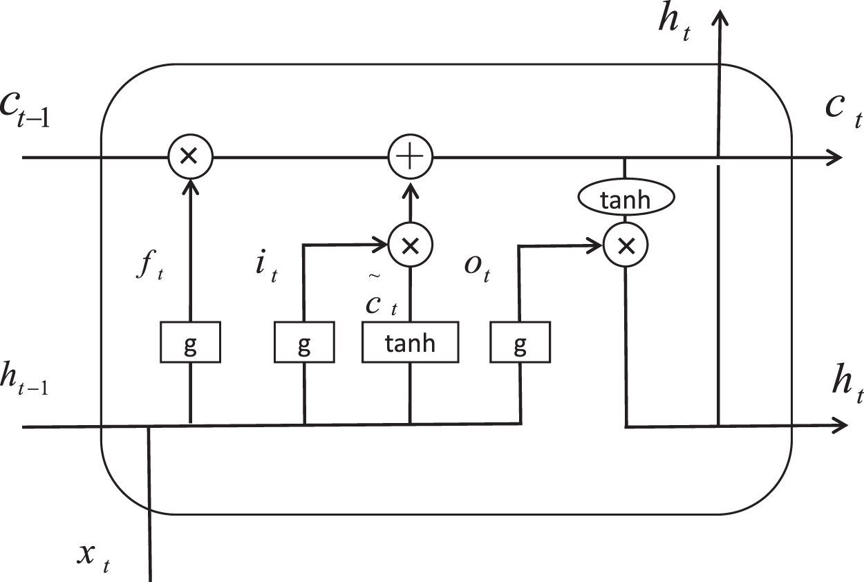
Schematic diagram of the internal structure of LSTM. LSTM, long short-term memory.

The g() in the formula represents the activation function, which is used to decide what information is allowed to pass. The range of g() is from 0 to 1. When g() is set to 1, it means that all information is allowed to pass. When g() is set to 0, it means that no information is allowed to pass. The tanh() stands for hyperbolic tangent function, which is used to control new information, that is, how much new information is reflected, and the range is −1 to +1. w and v are a weight matrix, and b stands for bias. h_t − 1 represents the output at the previous moment, and x_t represents the input at the current moment. Among them, the forget gate is marked as f_t, the input gate is marked as i_t, and the output gate is marked as o_t. x_t and h_t − 1 are input to the three gates labeled f_t, i_t, and o_t. One of the differences between RNN and LSTM is that there is an extra conveyor belt named “cell state” at the top of LSTM, which is marked as c in Figure 1 and used to memorize information.

The LSTM neural network is a special RNN, which applies memory function in the network model. For example, we decompose an article, and each sentence is a training object. X[i] represents the i-th sentence, and each word in each sentence represents a time step. X[i][0] means the first word in the i-th sentence. The information of this word can be memorized and passed to the fifth word X[i][4]. It can be seen that the memory function of LSTM works in one sentence.

Convolutional neural network

CNNs tend to have good image recognition results, such as handwritten digit recognition, input several pictures of handwritten digits, and repeatedly modifying the weight parameters through multiple CNN trainings. The resulting neural network model can accurately recognize handwritten digits. CNN includes convolutional layers, pooling layers, and fully connected layers. The convolution layer mainly extracts local features of the input data. The researcher defines a convolution kernel inside the convolution layer. Its shape is a square matrix that is used to extract a certain feature. The convolution kernel is multiplied by the corresponding bits of the digital input matrix and then added to obtain the output value of a convolution layer. The higher the output value, the higher the degree of matching between the two. Because one convolution kernel recognizes one feature and the input data may have multiple features, there may be numerous convolution kernels in one convolution layer to extract multiple features. Use the output of the obtained convolution layer as the input of the pooling layer. The pooling layer is mainly used to reduce the number of training parameters and reduce the feature vector output dimension by the convolution layer. The most common pooling layers are maximum pooling and mean pooling. In this article, we choose maximum pooling; that is, the maximum value in a specified area represents the entire area. The output value of the pooling layer is then expanded as the input of the fully connected layer to generate the final output.

Support vector machine

SVM is a machine learning algorithm for classification based on statistical learning theory. SVM is a convex quadratic optimization problem. It minimizes sample point errors and reduces model generalization capabilities by using the structural risk minimization criteria. The main goal of the SVM is to find a hyperplane to segment the sample so that there can be a larger gap between heterogeneous points closer to the hyperplane; that is, not all the sample points need to be considered, we need to maximize the distance between the points closest to the resulting hyperplane. It is widely used in handwritten digit recognition, image classification, text, and hypertext classification because SVMs can reduce the need for labeled training examples in standard induction.

A Proposed LSTM Framework with Leading Indicators

In this section, the process proposed by the LSTMLI framework and the data initialization process are specifically introduced. This thesis mainly studies the impact of leading indicators on the stock market, and so, two leading indicators of futures and options are used for experiments. In this chapter's first subsection is a brief introduction to the data set used in the experiment. The second section is to initialize the data set and use the processed data as the input of the framework. The third part is the specific process of the framework proposed in this article.

Data set

The data sets used in the experiment are historical data, futures, and options. In financial markets, stock prices are affected not only by historical behavior but also by leading indicators. Leading indicators can reflect the state of future economic development and are indicators that will change before economic growth or recession. Leading indicators are also called predictive indicators, which can provide predictive information for future economic conditions. Using this indicator, researchers can know the turning point of the economy in advance, to adopt appropriate trading strategies. For example, when the monetary authorities reduce the money supply, on the one hand, it shows the policy intentions of the authorities, implying the current trend of overheating in the economy. On the other hand, it will bring an increase in interest rates, which will increase the cost of enterprises and reduce profits, thereby reducing the attractiveness of investors. The increase in interest rates increases the opportunity cost of stock investment, which inevitably leads to a reduction in investment and a decline in stock prices. Therefore, this study focuses on the correlation between the two leading indicators of futures and options and the stock market and uses leading indicators to predict the trend of stock prices.

As a particular trading method, futures trading has undergone two complex evolutionary processes from the beginning of spot trading to forward trading and then from forward trading to futures trading. To put it simply, futures are not a spot but a standardized contract. The purpose of futures trading is generally not to obtain physical objects at maturity but to buy and sell futures contracts. Time, quantity, and quality are the three elements of this standardization, that is, a contract that delivers a fixed quantity and a certain quality of a certain quality at a specific time. The futures exchange uniformly formulates futures contracts. The delivery period of futures is placed in the future. It can be 1 week, 1 month, or even 1 year later. The corresponding spot can be a financial instrument, such as bonds and foreign exchange. It can also be a commodity, such as soybeans or crude oil. Options are similar to futures and are also a contract. The option is generated based on futures. When the option is traded, the party who buys the option is called the buyer, the assignee of the right, and the party who sells the option is called the seller, the obligor who must perform the buyer's exercise of the right. The difference between futures and options is that options give the buyer of the contract the right to buy or sell a predetermined number of commodities at the agreed price within the agreed period of the parties. It is a right to choose whether to execute or not in the future. In short, futures are one-way contracts, and options are two-way contracts. For example, we bought an option from an internet technology company for $50. In February 2020, the company gave us 1000 stocks at an exercise price of $10 per share and an exercise date of February 2021. That said, in February 2021, we could buy 1000 shares of the company for $10 a share. If the company's stock price reaches $15 per share when the exercise date is reached, then we choose to exercise our power to buy at $10 per share, which means that we have bought $15,000 stock with a market value of $10,000. Also, when the exercise date is reached, and the company's stock price is $5 per share, we will lose money if we exercise our power at this moment. Thus, we will then cancel to exercise our power, and will have $50 lose at this stage.

Five important indicators of historical price are often used: the opening price, lowest price, highest price, closing price, and volume for stock price analysis. The futures indicators used in our experiments include opening price, highest value, lowest value, closing price, and volume. The indicators of the options the test uses include volume, open interest, closing price, and settlement price.

First, let us look at a data set of five stocks in the Taiwan market. The five stocks are as follows: CDA, CFO, DJO, DVO, and IJO. Tables 1 –3 are the historical data, futures data, and options data of the five Taiwan stocks, respectively.

Table 1.

The historical prices of the five stocks

	d_i1	d_i2	d_i3	d_i4	d_i.
CDA	266	266	260	262.5	…
CFO	118	118	115	115	…
DJO	260	264	259	264	…
DVO	244.5	246.5	243	246.5	…
IJO	3825	3880	3630	3635	…

Table 2.

Futures data of the five stocks

	t_i1	t_i2	t_i3	t_i4	t_i.
CDA	262.5	265	265.5	262.5	…
CFO	117	117	117.5	117	…
DJO	163.5	262	263.5	258	…
DVO	246	244	246.5	243.5	…
IJO	3660	3815	3865	3635

Table 3.

Options data of the five stocks

	z_i1	z_i2	z_i3	z_i4	z_i.
CDA	5.2	70	7.3	11	…
CFO	3.25	20	0.51	15	…
DJO	14.85	1	0.27	1	…
DVO	3.4	2	6.85	2	…
IJO	297	0	30.1	0	…

d_i, t_i, z_i are the various factors that affect the stock price. d_i represents the open, high, low, close, or volatility attributes of the stock. t_i represents the current price, the opening price, the highest price, and the closing price of the futures. z_i represents the attributes of open interest and settlement price of options. Among them, options include buy options and sell options.

Data initialization

Before the experiment, input data need to be further processed, that is, to standardize the data. Because the experiment may be affected by the size of the data and the results are not ideal. First, standardize the original data to make the range of all data consistent. The processed data conform to the standard normal distribution and help improve the accuracy of the prediction. As shown in Equation (1). $x^{*} = (x - μ) ∕ σ$ (1)

where μ is the mean of all sample data, and σ is the standard deviation of all sample data. Taking Taiwan's stock data as an example to standardize historical data, futures, and options, the standardized data are shown in Table 4.

Table 4.

The historical prices of the five stocks after standardization

	d_i1	d_i2	d_i3	d_i4	d_i.
CDA	1.42711759	1.36374702	1.28817718	1.29732091	…
CFO	4.4408209	4.2911262	3.92386591	3.58357233	…
DJO	3.48827139	3.75538658	3.65931874	3.92310615	…
DVO	0.136035	0.09801487	0.17144214	0.18939852	…
IJO	0.0073875	0.02757984	0.05991671	0.07369991	…

The proposed LSTMLI framework

In this section, the proposed process of LSTMLI is first shown in the first subsession. It consists of an LSTM framework, a simple input example, and a detailed pseudocode. The second subsession in this part provides the exact definition of architecture for the input historical price, futures, and options.

LSTMLI framework

This article divides the data into two parts according to the testing/training ratio. Our experiments integrate 30-day stock data into a matrix, input it into the LSTMLI framework, and output three nodes, as shown in Figure 2. An example of an input matrix is shown in Table 5. The study defines the stock's ups and downs as a label for comparison with the predicted value. In addition, this study defines labels as three types: Raise, No Change, and Fall, and simply denoted as +0.01, 0, −0.01. The actual meaning is that the price of the stock has risen (risen more than 0.01%), fallen (fallen more than 0.01%), and has not changed significantly (keep the value between +0.01% and 0.01%), as shown in Equation (2). We note here that this example just provides historical prices as input data, and the detailed architectures of input data are shown in the following session.

FIG. 2.

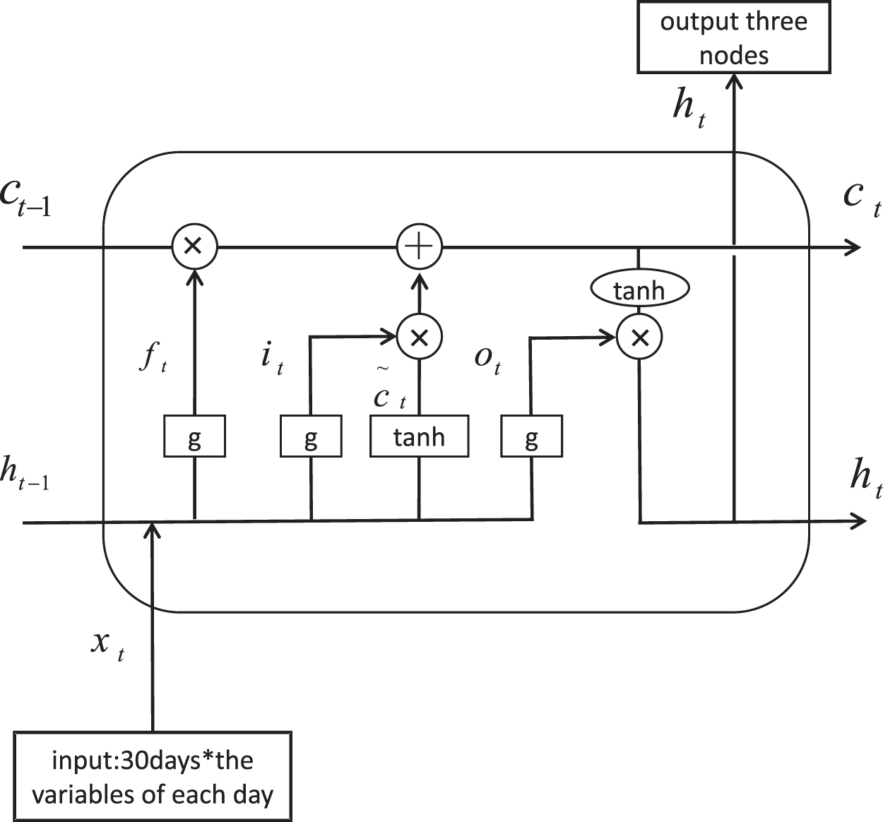
LSTMLI algorithm experiment flowchart. LSTMLI, LSTM with leading indicators.

Table 5.

Input matrix example

	1	2	3	…	30
Open	266	262	262	…	230
High	266	264	262.5	…	234.5
Low	260	261	257	…	230
Close	262.5	263	257.5	…	231.5
Quote change	−2.5	0.5	−0.5	…	0.5

l a b e l = \{\begin{matrix} c l a s s + 1, l > 0.01 \\ c l a s s 0, o t h e r s \\ c l a s s - 1, l < 0.01 \end{matrix}

(2)

Equation (2) is discussed around the rise and fall of stock prices. There are three output nodes (classes) in the proposed deep learning architecture as the final prediction results. Among them, l represents the value of the stock. When l is greater than or equal to 0.01, the label is defined as class +1. When l is less than −0.01, the label is defined as class −1. In other cases, the label is defined as class 0. Thus, the LSTMLI model will give a qualitative output based on the input data. For example, if the quoted change is −2.5, the expected output layer of these training data will be set as (0, 0, 1), where (+0.01: 0, 0: 0, −0.01: 1), and if the quote change is +2, it will be set as (1, 0, 0). Our experiments set the learning rate to 0.001; the weight randomly takes the specified number of values from the sequence that obeys the specified normal distribution and offset to a two-dimensional tensor. All elements of the tensor are filled with 0.1. The process of our experimental analysis is shown in Figure 3. The formal pseudocode of the proposed process is shown in Algorithm 1.

FIG. 3.

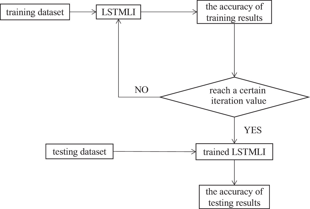
LSTMLI algorithm experiment flowchart.

Algorithm 1. The proposed LSTMLI framework and evaluation
Require: D is the data of training; K is the data of testing; z is the number of the maximum iteration as the terminal condition;
Ensure: the optimal weights w; evaluation result accuracy
1: initialize the input data D to D^∗ by Session 4.2 and 4.3.2
I > D^∗ is an input array for the information generated by historical prices, futures, and options and assume it consists of m input images
2: labeling each individual in D^∗ and generate the label array D_l
3: generate the initial weights w randomly for the LSTM network
4: for each round 1 to z do
5: for each round t = 1 to m does
6: input D_t^∗ to the proposed LSTM network and generate class label vector l
7: compare D^t and l to update w by Adam method²⁵
8: end for
9: end for
10: evaluate accuracy using the optimal weights w for testing data K
11: output w and accuracy

Algorithm 1 consists of both the training phase and the testing phase. The proposed model first initializes and normalizes the original input data into the input image array in Line 1. Note that the detail of the input architectures is shown in the following section. Then, each input unit in D* is labeled to the expected class in Line 2. The proposed method initials the weights for the LSTM network randomly in Line 3. The training process performs z time to optimize the weights w (Lines 4–9). In Lines 5 to 8, each input data in D* are inputted in the LSTM network and generate class label vector l (it is a three-value vector {0.98, 0.01, 0.01}) in Line 6. The proposed method compares the vector l and the expected vector D and uses an Adam optimizer,³⁸ which is a famous optimal updating method for deep learning neural networks, to update the weights w (Line 7). Finally, the proposed method evaluates the optimal weights w by the testing data K (Line 10) and outputs the results in Line 11.

Detail architectures of input images

In the proposed LSTMLI architecture, the input image is very complicated. Therefore, this section describes in detail the architecture of the input image used in the experiment. First, the futures, options, and historical prices generated images that are explained below. We note here that this section focuses on the data structure of the architecture; all values are standardized using the methods presented above.

Historical price image

From the above definitions, the image includes the opening price, lowest price, highest price, closing price, and volume of stocks within 30 days. The 30-day window is a width setting of the sliding windows for creating the input information. The proposed method will generate one input unit (image) for the whole input data by shifting the sliding windows. The following futures and options are both the same. The proposed method puts these values in a column in a certain order and expands them for 30 days as 30 columns to build an image. An example is shown in Figure 4.

FIG. 4.

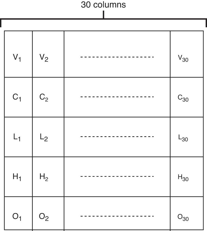
An example of the image established by historical prices (O_n, H_n, L_n, C_n, and V_n are the opening price, highest price, lowest price, closing price, and volume at n-th day).

Futures image

It includes opening price, highest value, lowest value, closing price, and volume, which are similar to historical prices. In addition, the products of the future of a particular underlying asset (stock) can have several different expiry dates. In the proposed framework, we choose a future whose three expiration dates are closest to the current date. We put the relevant attributes within 1 day of the futures in one column, and expand 30 days as a matrix. We can see this in Figure 5, which shows an example.

FIG. 5.

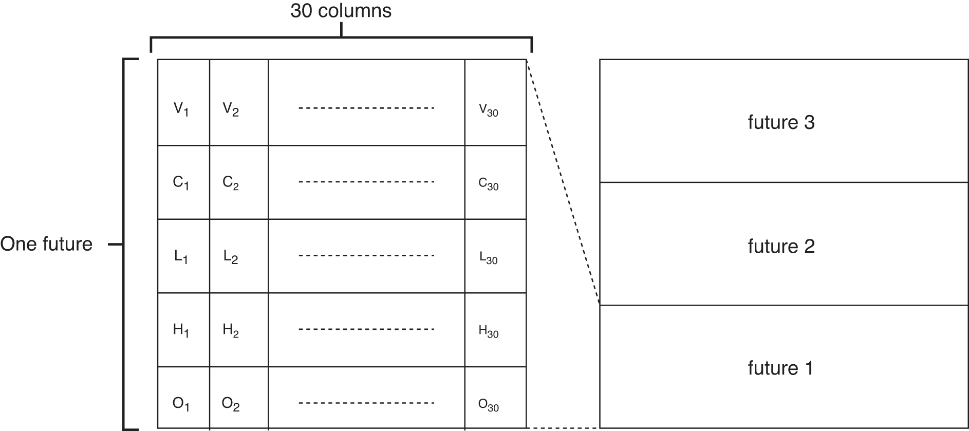
An example of the image established by futures (O_n, H_n, L_n, C_n, and V_n are the opening price, highest price, lowest price, closing price, and volume at n-th day).

Options image

Compared with futures and historical prices, the situation with options is more complicated. As is well known, there are two types of options (call options and put options) in the options market. In this study, we only select the near-month option data of stocks. In this method, 10 different options (10 call rights and 10 put rights) are selected, and its settlement price is closest to the current price of the stock while attributes are extracted from these options to construct an image. Attributes include volume, open interest, closing price, and settlement price. Its composition is similar to the previous two images, and the 30-day data are also expanded into a matrix. We can see this in Figure 6, which shows an example.

FIG. 6.

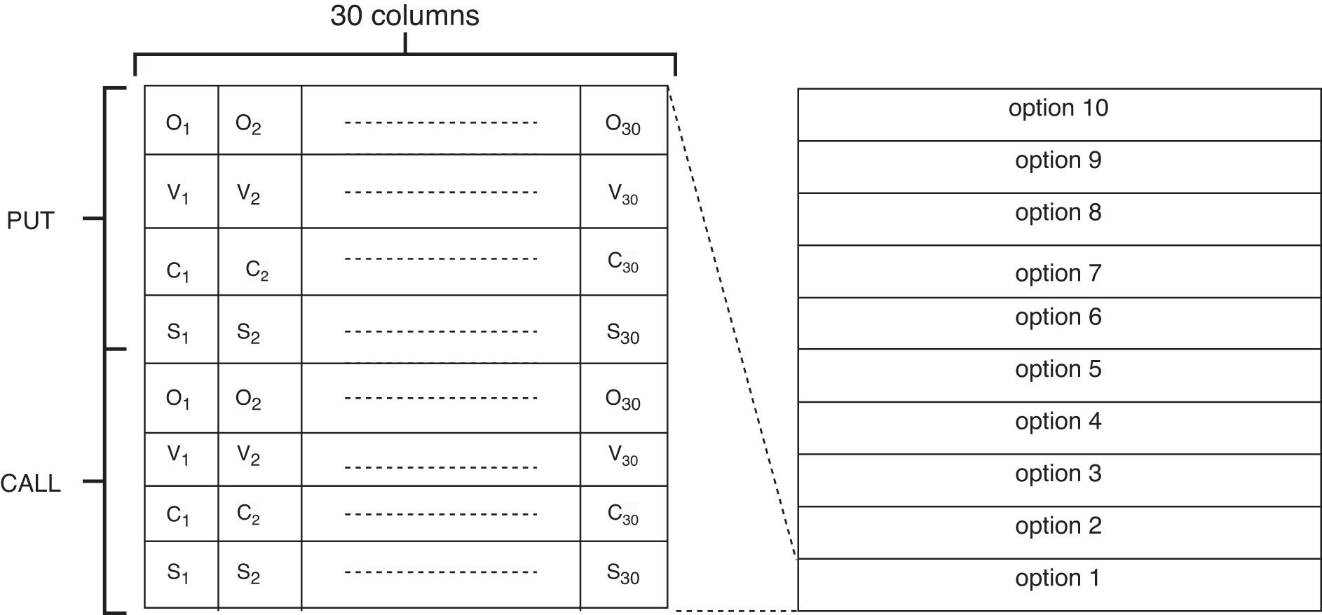
An example of the image established by options (S_n, C_n, V_n, and O_n are the settlement price, closing price, volume, and open interest at n-th day).

Combination image

The combined image is the final input form of the framework. It just includes the first three images to generate a new image, which contains information about historical prices, futures, and options. Figure 7 shows an example.

FIG. 7.

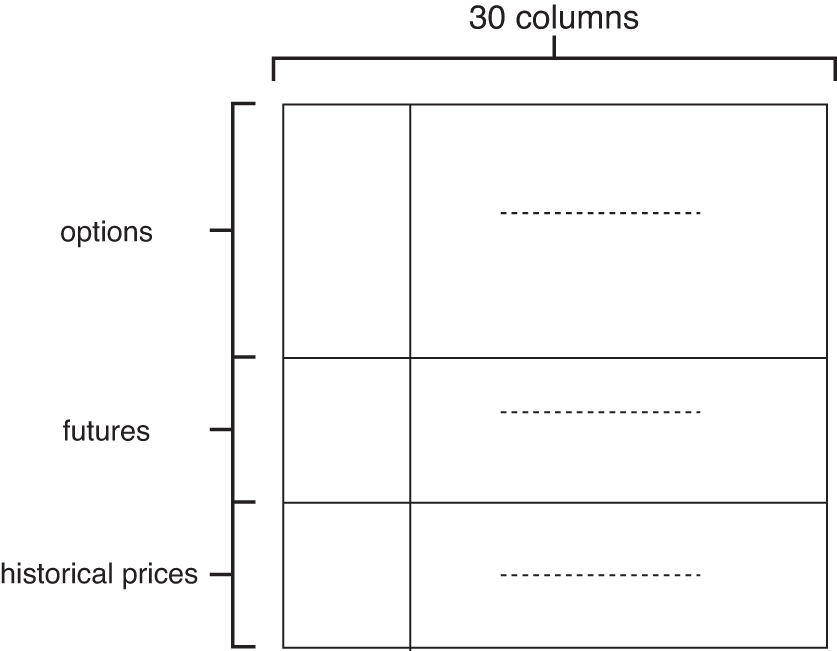
An example of the image established by combination data.

Experimental Results

Our experiments are mainly to study which model can better predict stock price fluctuation and study the effect of leading indicators on stock prices. The data used in the experiment are the Taiwan stock market data from September 28, 2018, to October 30, 2019, and the U.S. stock market data from September 28, 2018, to August 30, 2019. The research focuses on the two leading indicators of futures and options.

The specific experimental process is as follows. This article mainly studies which model can predict the stock price more accurately and study the effect of leading indicators on the stock price, thereby helping investors or investment companies obtain higher returns. The experiment divides the collected stock data into two parts, one for training data and one for testing data. To improve the accuracy of prediction results, we need to find a suitable ratio to divide the data set. Therefore, this experiment uses 40%, 50%, 60%, 70%, 80% of the data set as test data, and the corresponding training data are 60%, 50%, 40%, 30%, 20% of the data set. The remaining data parameters are unchanged to determine the optimal ratio. The study used the historical data of the Taiwan and U.S. stocks and obtained the following experimental results through multiple experiments, as shown in Table 6. Table 6 shows that when the ratio of training data to test data is 5:5, the resulting prediction accuracy is the highest.

Table 6.

Performance of the proposed algorithm with different proportions for the historical data sets of stocks

	40%	50%	60%	70%	80%
CDA	0.418322	0.47142857	0.45828	0.427577	0.43664
CFO	0.43853	0.5	0.449545	0.4643378	0.4696558
DJO	0.447281	0.48571429	0.462891	0.4574	0.453051
DVO	0.392358	0.41428571	0.401164	0.41095	0.4206703
IJO	0.420946	0.47142857	0.45711	0.454399	0.43567
AAPL	0.4092327	0.466101	0.437299	0.443747	0.435799
AMZN	0.4302049	0.5105	0.47999	0.4624633	0.48547
FB	0.410836	0.47032	0.45019	0.43667	0.428599
IBM	0.497061	0.558704	0.46916	0.4965567	0.47554
MSFT	0.470342	0.54013	0.46613	0.43675	0.48644

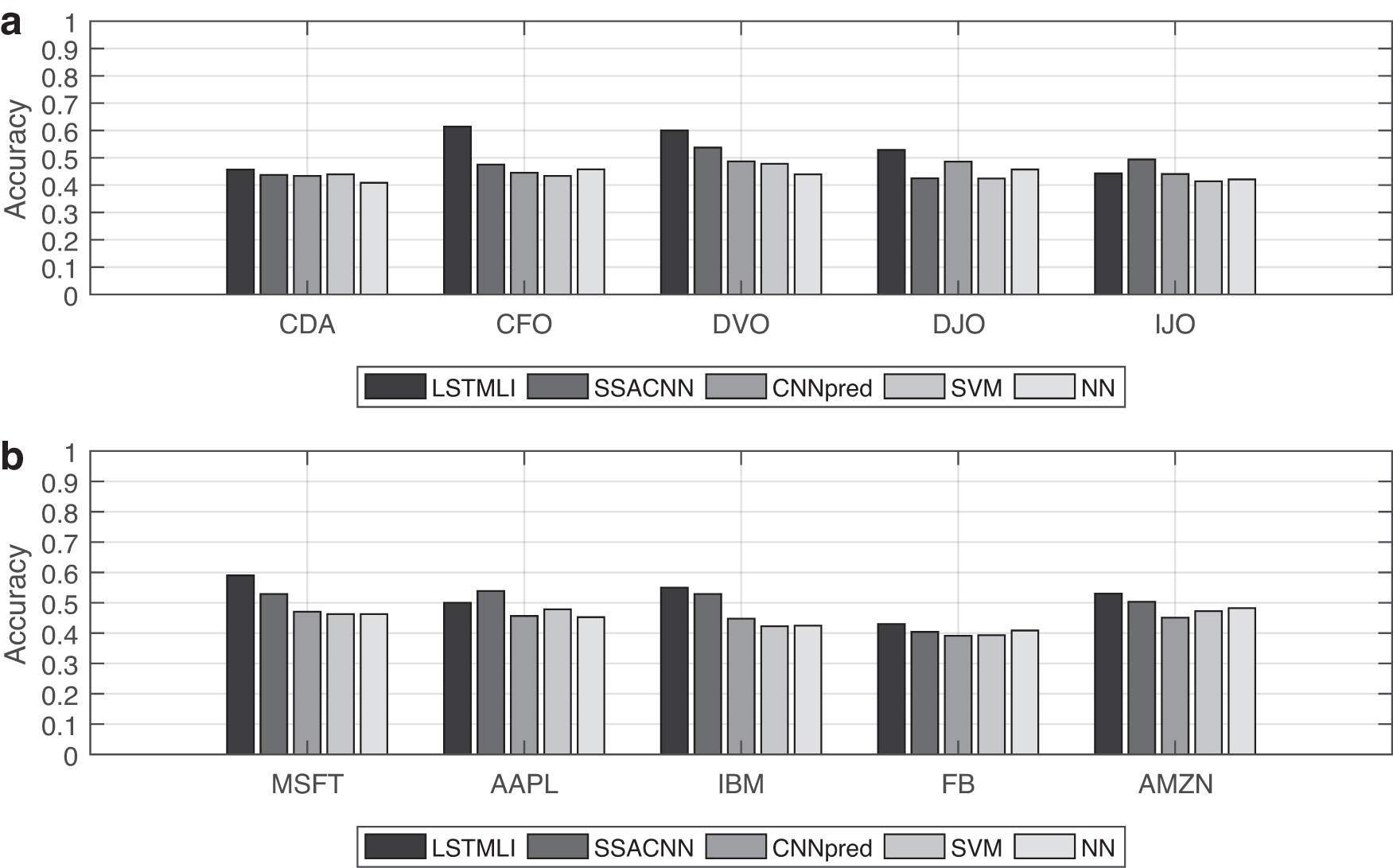
Next, the experiment uses only historical data to measure the predictive performance of LSTMLI relative to other models, including SSACNN, CNN-based stock market prediction (CNNpred), SVM, and neural network (NN). The test still only uses historical prices for the Taiwan and the U.S. stocks and then compares the accuracy of different prediction models between the same stocks. The experimental results are shown in Figure 8a and b. It can be seen that in the Taiwan stock market, the accuracy of LSTMLI prediction is higher than that of other models. In the U.S. stock market, the prediction performance of LSTMLI is much higher than other models.

FIG. 8.

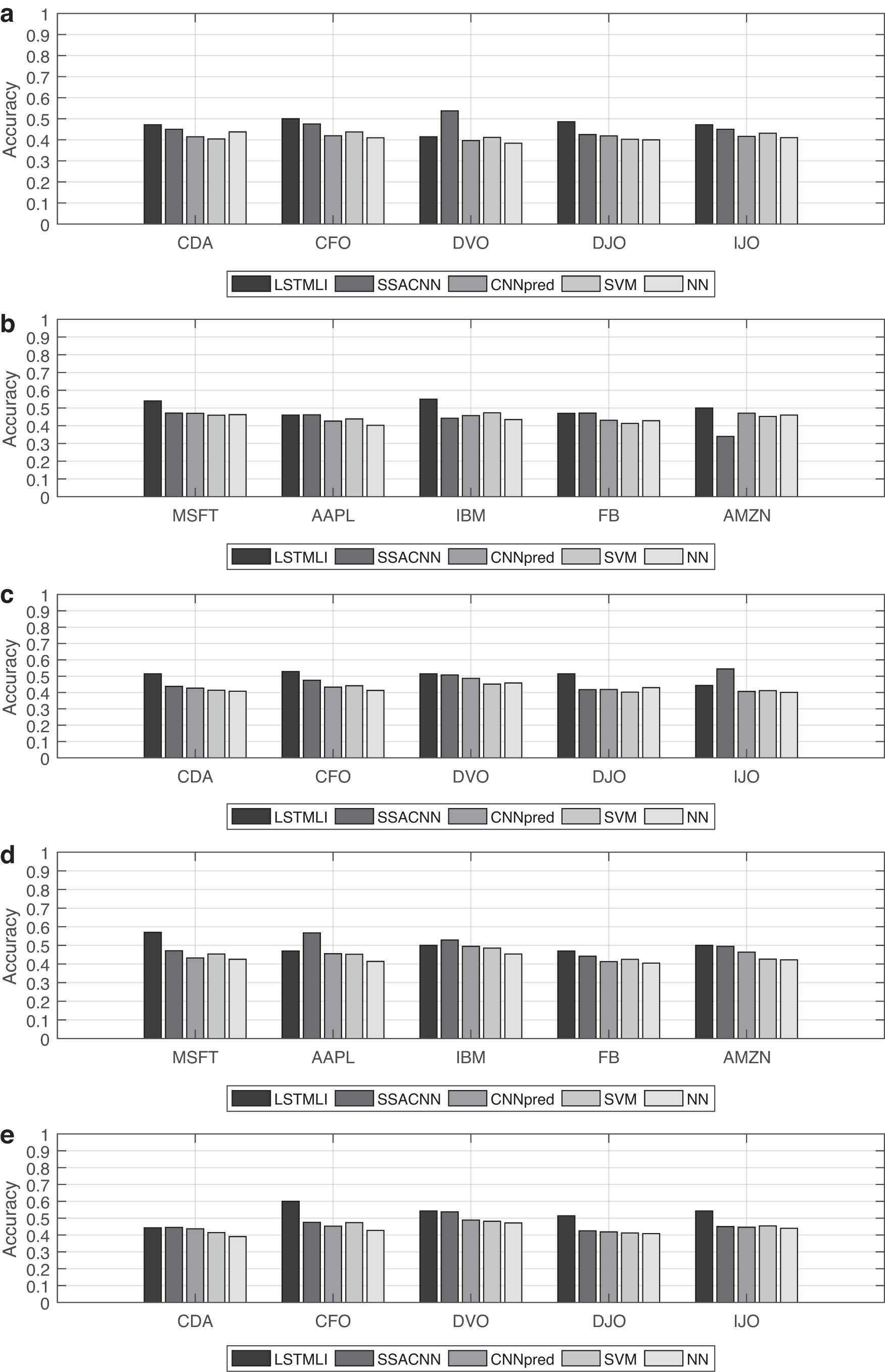
A bar chart of the accuracy of the prediction model using different data sets. (a) Use historical price as a data set in the Taiwan stock market. (b) Use historical price as a data set in the U.S. stock market. (c) Use options as a data set in the Taiwan stock market. (d) Use options as a data set in the U.S. stock market. (e) Use futures as a data set in the Taiwan stock market.

In the stock market, the impact of leading indicators on stock prices cannot be ignored. This study uses two leading indicators, futures, and options, to predict stock price fluctuations. The prediction methods used are LSTMLI, SSACNN, SVM, CNNpred, and NN. The experimental results we obtained using options for prediction are shown in Figure 8c and d. The experiment compares the accuracy achieved by different models using the same stock for prediction. Obviously, in Taiwan's stock market, the prediction accuracy of LSTMLI is much higher than that of other models. Similarly, in the U.S. stock market, the prediction performance of LSTMLI is also relatively good. The experimental results obtained by our futures forecast are shown in Figure 8e. Because there is no leading indicator of futures in the U.S. stock market, the study only conducts experiments on the Taiwan stock market. It can be seen from Figure 8e that the accuracy obtained by using LSTMLI for prediction is relatively high.

Our experiments use the Taiwan and the U.S. stock markets. To be able to predict stock price fluctuations more accurately, we combine the historical prices of stocks with leading indicators. Because there is no leading indicator of futures in the U.S. stock market, the test only combines historical data with options. Taiwan's stocks, combine three types of data. This article uses LSTMLI, SSACNN, CNNpred, SVM, and NN to make predictions. The experimental results obtained are shown in Figure 9. By comparing the accuracy obtained by different prediction models of the same stock, it can be found that, whether it is the Taiwan stock market or the U.S. stock market, the accuracy obtained by LSTMLI prediction is the highest compared with other models.

FIG. 9.

A bar chart of the accuracy of the forecast model using historical prices and leading indicators. (a) The stocks of Taiwan. (b) The stocks of the United States.

To study the effect of leading indicators on the stock price, in the case of using only the LSTMLI model, we compare the prediction results obtained from the data set that uses only historical data and only the leading indicators, and that combines historical data with leading indicators.^39,40 The experimental results are shown in Figure 10. Overall, when only historical data are used for forecasting, the results obtained are relatively low. When using futures or options as the data set, the accuracy obtained is generally higher than that obtained using historical data. For example, in Figure 10a, on the stock CDA, the value obtained using futures is higher than the value obtained using historical data. On the stock CFO, DVO, and DJO, the values obtained by using futures and options, respectively, are higher than those obtained by using historical data. On the stock IJO, the value obtained using options is higher than the value obtained using historical data.

FIG. 10.

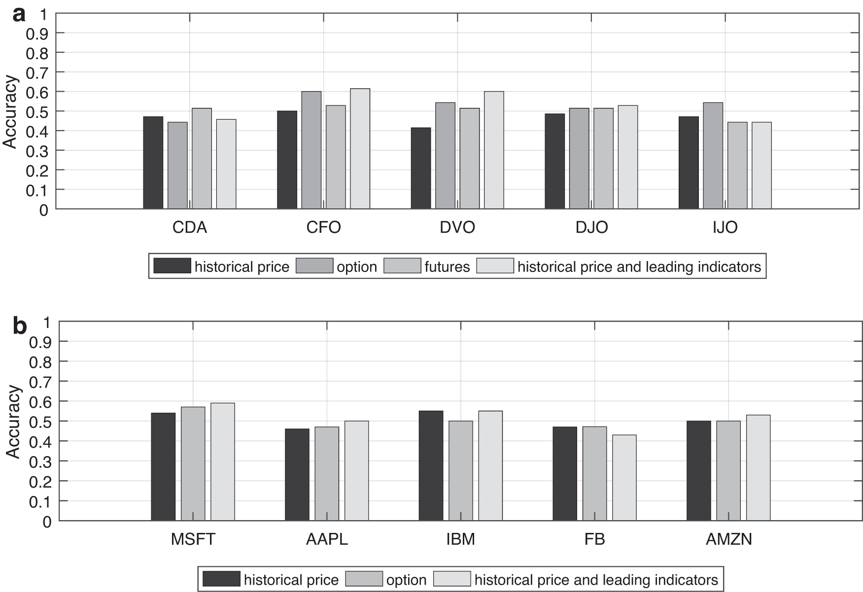
A bar chart of the prediction accuracy obtained by adding the leading indicator data set and a single historical data using only the LSTMLI model. (a) The stocks of Taiwan. (b) The stocks of the United States.

From the above experiments, it can be seen that, whether in the Taiwan stock market or the U.S. stock market, the prediction performance of the LSTMLI is better than other models, and the prediction accuracy obtained by adding the data set of leading indicators is higher. In this research, the LSTMLI framework is proposed based on leading indicators such as futures and options. Because the leading indicators can reflect the future economic development, and the LSTM model itself has good performance in terms of prediction, the proposed LSTMLI framework has higher accuracy than SSACNN, CNNpred, SVM, and NN.

Conclusion

In this study, our research mainly studied the predictive performance of various models. To reduce useless information, in this article, instead of inputting the data one by one into the model, the data are integrated into a matrix and then used as input in the form of a matrix. In other words, the input to the model in the article is an image. Besides, the output of the model adopts a classification method, which divides the rise and fall of stocks into three categories: +0.01, 0, −0.01, respectively. That is, the predicted stock price is no longer a specific value but a category. This study compares LSTMLI with other models, and the experimental results show that the prediction accuracy obtained with the LSTMLI model is higher. Unlike the previous stock forecasts, this article adds leading indicators when training the model with LSTMLI, which has a certain effect on stocks' volatility. The research results show that the data set with leading indicators is more accurate than the prediction obtained by using only historical data. However, in this study, only the two leading indicators of futures and options are used, and many factors affect stock prices. This requires us to study further to predict the stock price more accurately. Finally, the contribution of this research is that the LSTMLI model trained on the data set with leading indicators greatly improves the accuracy of the prediction.

Footnotes

Author Disclosure Statement

No competing financial interests exist.

Funding Information

No funding was received for this article.

Abbreviations Used

References

Kim

, Kim

. Forecasting stock prices with a feature fusion LSTM-CNN model using different representations of the same data. PLoS One, 2019; 14: e0212320.

Samuelson

PA.

Lifetime portfolio selection by dynamic stochastic programming. Stochastic Optim Models Finance, 1975; 15:517–524.

Brooks

Predicting stock index volatility: Can market volume help?. J Forecasting, 1998; 17:59–80.

Keim

, Stambaugh

. Predicting returns in the stock and bond markets. J Financ Econ, 1986; 17:357–390.

Malkiel

, Fama

. Efficient capital markets: A review of theory and empirical work. J Finance, 1970; 25:383–417.

Hiew

JZG

, Huang

, Mou

, et al. Bert-based financial sentiment index and LSTM-based stock return predictability. arXiv 2019;1906.09024.

Baker

, Wurgler

. Investor sentiment and the cross-section of stock returns. J Finance, 2006; 61:1645–1680.

Lee

, Shleifer

, Thaler

. Investor sentiment and the closed-end fund puzzle. J Finance, 1991; 46:75–109.

Han

Investor sentiment and option prices. Rev Financ Stud, 2008; 21:387–414.

10.

Cowles 3rd

Can stock market forecasters forecast? Econometrica J Econometric Soc 1933:1:309–324.

11.

Borovkova

, Tsiamas

. An ensemble of LSTM neural networks for high-frequency stock market classification. J Forecasting, 2019; 38:600–619.

12.

Bao

, Yue

, Rao

. A deep learning framework for financial time series using stacked autoencoders and long-short term memory. PLoS One, 2017; 12:0180944.

13.

Huang

, Nakamori

, Wang

. Forecasting stock market movement direction with support vector machine. Comput Oper Res, 2005; 32:2513–2522.

14.

Nayak

, Mishra

, Rath

. A na¨ıve SVM-KNN based stock market trend reversal analysis for Indian benchmark indices. Applied Soft Computing, 2015; 35:670–680.

15.

Cortes

, Vapnik

. Support-vector networks. Mach Learn, 1995; 20:273–297.

16.

Sheta

, Ahmed

SEM

, Faris

. A comparison between regression, artificial neural networks and support vector machines for predicting stock market index. Soft Comput, 2015; 7:2.

17.

Tian

, Chu

, Pan

, et al. A compact pigeon-inspired optimization for maximum short-term generation mode in cascade hydroelectric power station. Sustainability, 2020; 12:767.

18.

Kimoto

, Asakawa

, Yoda

, Takeoka

. Stock market prediction system with modular neural networks. In: 1990 IJCNN International Joint Conference on Neural Networks. San Diego, CA: IEEE, 1990. pp. 1–6.

19.

Hinton

, Osindero

, Teh

. A fast learning algorithm for deep belief nets. Neural Comput, 2006; 18:1527–1554.

20.

Henrique

, Sobreiro

, Kimura

. Literature review: Machine learning techniques applied to financial market prediction. Expert Syst Appl, 2019; 124:226–251.

21.

Chen

, Zhou

, Dai

A LSTM-based method for stock returns prediction: A case study of china stock market. In: IEEE International Conference on Big Data. Santa Clara, CA: IEEE, 2015. pp. 2823–2824.

22.

Fischer

, Krauss

. Deep learning with long short-term memory networks for financial market predictions. Eur J Oper Res, 2018; 270:654–669.

23.

Naik

, Mohan

. Study of stock return predictions using recurrent neural networks with LSTM. In: International Conference on Engineering Applications of Neural Networks. Crete, Greece: Springer, 2019. pp. 453–459.

24.

Gunduz

, Yaslan

, Cataltepe

. Intraday prediction of borsa istanbul using convolutional neural networks and feature correlations. Knowledge-Based Syst, 2017; 137:138–148.

25.

Hoseinzade

, Haratizadeh

. Cnnpred: CNN-based stock market prediction using a diverse set of variables. Expert Syst Appl, 2019; 129:273–285.

26.

Chen

, Yeo

, Lau

, Lee

. Leveraging social media news to predict stock index movement using RNN-boost. Data Knowl Eng, 2018; 118:14–24.

27.

Ding

, Qin

. Study on the prediction of stock price based on the associated network model of LSTM. Int J Mach Learn Cybern, 2020; 11:1307–1317.

28.

Yadav

, Jha

, Sharan

. Optimizing LSTM for time series prediction in Indian stock market. Procedia Comput Sci, 2020; 167:2091–2100.

29.

Kim

, Han

. Genetic algorithms approach to feature discretization in artificial neural networks for the prediction of stock price index. Expert Syst Appl, 2000; 19:125–132.

30.

Zheng

, Jiang

, Long

. Exchange rates change, asset-denominated currency difference and stock price fluctuation. Appl Econ, 2019; 51:6517–6534.

31.

French

, Schwert

, Stambaugh

. Expected stock returns and volatility. J Financ Econ, 1987; 19:3.

32.

Ormoneit

, Neuneier

Experiments in predicting the German stock index DAX with density estimating neural networks. In: IEEE/IAFE Conference on Computational Intelligence for Financial Engineering. New York, NY: IEEE, 1996. pp. 66–71.

33.

Kim

, Won

. Forecasting the volatility of stock price index: A hybrid model integrating LSTM with multiple GARCH-type models. Expert Syst Appl, 2018; 103:25–37.

34.

Di Persio

, Honchar

. Artificial neural networks architectures for stock price prediction: Comparisons and applications. Int J Circuits Syst Signal Process, 2016; 10:403–413.

35.

JMT

, Li

, Srivastava

, et al. A graph-based convolutional neural network stock price prediction with leading indicators. Software Pract Experience, 2020; 51:628–644.

36.

Nelson

, Pereira

, de Oliveira

. Stock market's price movement prediction with LSTM neural networks. In: International Joint Conference on Neural Networks. Anchorage, AK: IEEE, 2017. pp. 1419–1426.

37.

Liu

Novel volatility forecasting using deep learning—Long short term memory recurrent neural networks. Expert Syst Appl, 2019; 132:99–109.

38.

Kingma

, Ba

Adam: A method for stochastic optimization. arXiv 2014;1412.6980 2014.

39.

JM-T

, Li

, Srivastava

, et al. A CNN-based stock price trend prediction with futures and historical price. In: 2020 International Conference on Pervasive Artificial Intelligence (ICPAI). Taipei, Taiwan: IEEE, 2020.

40.

JM-T

, Li

, Srivastava

, et al. A tool based on ML-driven graphical model for stock price prediction by leading indicators. IFAC-PapersOnLine, 2020; 53:692–697.