Applications of Bayesian Neural Networks in Outlier Detection

Abstract

Anomaly detection is crucial in a variety of domains, such as fraud detection, disease diagnosis, and equipment defect detection. With the development of deep learning, anomaly detection with Bayesian neural networks (BNNs) becomes a novel research topic in recent years. This article aims to propose a widely applicable method of outlier detection (a category of anomaly detection) using BNNs based on uncertainty measurement. There are three kinds of uncertainties generated in the prediction of BNNs: epistemic uncertainty, aleatoric uncertainty, and (model) misspecification uncertainty. Although the approaches in previous studies are adopted to measure epistemic and aleatoric uncertainty, a new method of utilizing loss functions to quantify misspecification uncertainty is proposed in this article. Then, these three uncertainty sources are merged together by specific combination models to construct total prediction uncertainty. In this study, the key idea is that the observations with high total prediction uncertainty should correspond to outliers in the data. The method of this research is applied to the experiments on Modified National Institute of Standards and Technology (MNIST) dataset and Taxi dataset, respectively. From the results, if the network is appropriately constructed and well-trained and model parameters are carefully tuned, most anomalous images in MNIST dataset and all the abnormal traffic periods in Taxi dataset can be nicely detected. In addition, the performance of this method is compared with the BNN anomaly detection methods proposed before and the classical Local Outlier Factor and Density-Based Spatial Clustering of Applications with Noise methods. This study links the classification of uncertainties in essence with anomaly detection and takes the lead to consider combining different uncertainty sources to reform detection outcomes instead of using only single uncertainty each time.

Introduction

Anomaly detection is a technique to identify present or future observations that do not conform to an expected pattern or the distribution of other items in a dataset (called outliers). It is an important issue in machine learning and has widespread applications in cyber security and e-crime detection,¹ such as malicious content removal,² fraud detection,³ and so on. Anomaly detection can be classified into outlier detection and novelty detection. Novelty detection is to detect whether a new observation is an outlier based on pure training data, which is a semi-supervised learning problem.^{4, P461} Outlier detection, on which this article mainly focuses, is to detect outliers among training data directly, which is an unsupervised learning problem.^{4, P461} For outlier detection, various algorithms had been developed, such as Local Outlier Factor (LOF),⁵ Density-Based Spatial Clustering of Applications with Noise (DBSCAN),⁶ and Isolation Forest.⁷

With the surge of available data and the improvement of hardware performance nowadays, Neural Networks (NNs), which are suitable for big data and large-scale computer vision tasks, have received unprecedented attention.^{8, Ch1} Therefore, how to use NNs to perform anomaly detection is an emerging research topic in recent years. Standard NNs are supervised learners, whose outputs are deterministic, and so they cannot classify something unexpected. Nevertheless, if we consider weight parameters in NNs as random variables that have certain distributions and use Bayesian inference strategy, the uncertainties and confidence levels for the predictions of NNs can be measured, and so unexpected items can be identified.

The measurement of uncertainties for model predictions has been discussed previously. There are totally three kinds of uncertainty that we can model: epistemic uncertainty, aleatoric uncertainty, and (model) misspecification uncertainty,⁹ whose specific meanings will be introduced in Measurement of Different Kinds of Uncertainties section. Kendall and Gal illustrated how to capture epistemic and aleatoric uncertainty in computer vision tasks under Bayesian deep learning frameworks.¹⁰ Besides, Kwon et al proposed a method of quantifying epistemic and aleatoric uncertainty in classification situations based on Bayesian neural networks (BNNs) and calculated these uncertainties using this method on some datasets.¹¹ To the best of our knowledge, the only study that systematically described misspecification uncertainty and measured it in time series predictions is presented by Zhu and Laptev.⁹

However, the shortcomings of their encoder-decoder method of calculating misspecification uncertainty are that it is merely effective for time series data and the outcome is mixed with epistemic uncertainty. In addition, all the research mentioned previously did not involve anomaly detection. On the contrary, for previous studies on anomaly detection with BNNs, only some piecemeal indices were used as uncertainty measurement to detect outliers, and they were neither linked to the classification of different uncertainties in essence nor unified in theory. For example, Pawlowski et al utilized a quantity called “disagreement” defined by Lakshminarayanan et al¹² as the measure of uncertainty,¹³ which is essentially epistemic uncertainty, and so only one kind of uncertainty was considered in their research. Moreover, Chen et al used three indices, Monte Carlo (MC) sampling variance, prediction entropy, and mutual information to detect anomalies, where the samples with high level of any index were picked out for reevaluation.¹⁴

The authors found that MC sampling variance and mutual information always had extremely similar fluctuation trends.¹⁴ It is because they are all the measurement of epistemic uncertainty in essence, and so only one of them is necessary to use. Besides, prediction entropy is actually a measure of aleatoric uncertainty. In addition, they treated anomaly detection as a binary classification problem, but this processing mechanism cannot cope with the situation that a training set in which all the anomalies are correctly labeled is not available, such as outlier detection, an unsupervised problem.

Inspired by those, this article aims to construct a bridge between the measurement of all kinds of uncertainties generated in model predictions and outlier detection, and propose a general method of outlier detection using BNNs based on uncertainty measurement that is applicable to a wide range of cases. In principle, the ideas of the anomaly detection methods used in Refs.^13,14 are only special cases of our method. The main contributions of this article are summarized as follows:

A widely applicable method of outlier detection with BNNs is proposed. It is based on the measurement of different kinds of uncertainties. For anomaly detection, previous studies usually only consider piecemeal indices as the measure of uncertainty. Unlike them, we classify different uncertainty measurement methods theoretically and use models to combine different kinds of uncertainties together to significantly improve the performance of the method. Linear combinations are utilized in this article and the experimental results show that good effects can be achieved if the parameters are carefully tuned, although more complicated models can be investigated.

A practical method to quantify model misspecification uncertainty is put forward in this article. The key idea is to utilize the loss function. For this kind of uncertainty, there is no feasible quantification method yet. Moreover, we also outline the methods of quantifying epistemic and aleatoric uncertainty in both regression and classification scenarios separately.

The method of this study is applied to different types of datasets. More concretely, we perform outlier detection on both Modified National Institute of Standards and Technology (MNIST) dataset and Taxi dataset using this method to illustrate its effectiveness and broad applicability.

The proposed method is widely compared with other anomaly detection methods. Specifically, to confirm superiority, we compare this method with the BNN anomaly detection methods proposed before, which only consider some piecemeal indices, and the LOF and DBSCAN methods. The results demonstrate that the performance of our method is more powerful compared with the previous BNN methods and is superior to those traditional methods like LOF and DBSCAN.

In the next section, we give an overview about the concept of BNN, and illustrate how to quantify different kinds of uncertainties and perform outlier detection based on uncertainty measurement. In Outlier Detection on MNIST Dataset Using BCNN and Outlier Detection on Taxi Dataset Using BLSTMNN sections, we will, respectively, train a Bayesian convolutional neural network (BCNN) for a handwritten digital image dataset (MNIST) and a Bayesian long short-term memory neural network (BLSTMNN) for a time series dataset (Taxi). We present our findings of outlier detection on these datasets separately. In addition, the performance of our method are compared with that of the previous BNN detection methods and the LOF and DBSCAN methods, respectively. Finally, the results of this article are summarized, possible limitations are discussed, and some advice for future work is put forward.

All experiments were conducted by Python 3.7 in this article. The main packages that we used to construct BNNs and process data were tensorflow (2.4.1), tensorflow.keras (2.4.0), tensorflow_probability (0.12.2), edward2 (0.0.2), and sklearn (0.23.2). We fixed a different random seed for each experiment to make the results reproducible. The Python code and data files for all the experiments are available at the online Github repository.¹⁵ In the code, we also visualized the confidence intervals for the predictions of BNNs and conducted some additional data analyses, and so on.

Methods

In this section, an introduction to the methods that will be used is put forward.

Bayesian neural network

First, let us introduce the principle of BNNs trained with the variational inference method. The ideas to build different types of BNNs are completely similar.

Assume that the training data are $D = (X, Y)$ , where X = {x₁,…,x_N} and Y = {y₁,…,y_N} are the inputs and labels respectively, and denote the weight parameters of the network by ω. First, we need to place a prior distribution p(ω) on ω. Denote the model likelihood by p(y|x,ω). Then, we can obtain the posterior of ω: $p (ω ∣ D) = \frac{p (D ∣ ω) p (ω)}{p (D)} = \frac{\prod_{i = 1}^{N} p (y_{i} ∣ x_{i}, ω) p (ω)}{p (Y ∣ X)} .$ (1)

Consequently, the posterior predictive distribution can be obtained⁹:

where x* and y* are the new input and output, respectively. However, the posterior Eq. (1) is intractable to calculate, because the marginal likelihood p(Y|X) cannot be evaluated analytically.

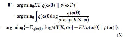
To train the BNN model, the variational inference approach¹⁶ is widely used. We need to find a tractable variational approximation to the posterior of the weights, say q(ω|θ), and then find the parameter θ that minimizes the Kullback–Leibler (KL) divergence with the true posterior^11,17:

Afterward, MC samples drawn from q(ω|θ) can be used to estimate the integral Eq. (2). Under the framework of BNN, the multivariate Gaussian distribution with trainable means, variances, and covariances is usually used as the approximate posterior q(ω|θ) because of its high computational efficiency and effectiveness in approximation.^18–20 Let

It is the loss function for training the BNN model and called Negative Evidence Lower Bound (−ELBO).^11,17 The first term of $ℱ (D, θ)$ is a data-dependent part, which is referred to as the likelihood cost, and the second term is a prior-dependent part, which is referred to as the complexity cost.¹⁷

Measurement of different kinds of uncertainties

Now, we are going to introduce the method of quantifying different kinds of uncertainties under the framework of BNNs in both regression and classification scenarios.

Recall that the uncertainty in model predictions can be decomposed into three independent parts: epistemic uncertainty, aleatoric uncertainty, and (model) misspecification uncertainty.⁹ Epistemic uncertainty, also called model uncertainty, accounts for the uncertainty about model parameters, that is, our ignorance about which model generated our data.^9,10 It measures the consistency (or stability) of the model's output for each sample at different times. This uncertainty is caused by insufficient training data and it can vanish given enough data. Aleatoric uncertainty captures the irreducible noise inherent in data or data generation processes.^9,10 This uncertainty measures the model's confidence in its prediction to each sample. It cannot be reduced even if more data are collected. The third kind of uncertainty, model misspecification, captures the circumstance that a sample comes from a different distribution than the cluster of the training set.⁹

The methods in Zhu and Laptev⁹ and part of the methods in Chen et al¹⁴ will be used to quantify epistemic and aleatoric uncertainty. It is because they can not only capture the nature of these two uncertainties, but also have low computational complexity. However, other methods, like the approaches in Refs.,^10–12 can also be used and similar results will be obtained, as long as the two conditions are satisfied: the correspondence between the quantification method and the meaning of the uncertainty; the independence between each kind of uncertainty. For misspecification uncertainty, we will propose a new method of utilizing the loss function to quantify it.

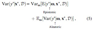
Based on the notations defined in Bayesian Neural Network section, further denote the NNs as function f^ω(·), where f stands for the network architecture and ω represents the weight parameters. Then, given the weight ω, the prediction of the NNs to any observation x is f^ω(x). The benefits of this notation are that it can represent which network processes the data and the conditional on the weight parameters of the network. According to Zhu and Laptev,⁹ the epistemic and aleatoric uncertainty of the model prediction y* for a new sample x* can be quantified by the variance of the predictive distribution Eq. (2), which can be further decomposed using law of total variance:

where the first term reflects the uncertainty about $ω$ , which is epistemic uncertainty, and the second term measures the noise inherent in data, which is aleatoric uncertainty. If the dimension of y* is more than 1, all the variance in Eq. (5) should be regarded as the sum of the variance of each component of the corresponding vector.

In regression, we usually assume that the model likelihood is independent Gaussian distribution⁹: $y ∣ x, ω \sim N (f^{ω} (x), σ_{ω}^{2}),$ (6)

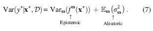
where y is the model prediction, and σ_ω > 0 is the standard deviation of the Gaussian distribution that depends on the weight $ω$ . Then, Eq. (5) can be written as follows:

We can estimate Eq. (7) using MC samples drawn from the variational posterior q(ω|θ).

In classification, the likelihood is usually modeled as independent one-hot categorical distribution with C ≥ 1 categories²¹ (see Appendix A1 for details): $y ∣ x, ω \sim O n e H o t C a t e g o r i c a l (p^{ω} (x)),$ (8)

where y is the model prediction and $p^{ω} (x) = {(p_{1}^{ω} (x), p_{2}^{ω} (x), \dots, p_{C}^{ω} (x))}^{T}$ is the probability vector for each class given the weight ω and input x. In classification, to estimate aleatoric uncertainty, instead of using the second term in Eq. (5), we adopt the expectation of the entropy of p^ω(x). They all can capture aleatoric uncertainty but utilizing the entropy is more robust. This mechanism is inspired by the method of prediction entropy proposed in Chen et al¹⁴ with a little modification as the original method has some overlap with epistemic uncertainty. Then, the epistemic and aleatoric uncertainty in classification scenarios can be written as follows:

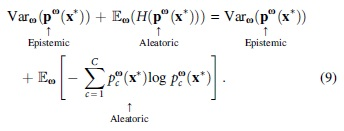
We can also use MC samples from q(ω|θ) to estimate the two terms in Eq. (9).

Furthermore, in anomaly detection, we also need to capture the uncertainty arisen from predicting unusual samples. Therefore, the complete measurement of prediction uncertainty should also include model misspecification uncertainty. At present, there are no simple and pragmatic approaches to measure this uncertainty yet. Herein, we propose a new method to quantify it. The main idea is to use the expectation of the loss function with respect to the weight parameter ω, because the loss can be a measure of abnormality levels of observations. In regression, we often use mean-squared error (MSE) as the loss function, and so model misspecification uncertainty can be quantified as follows:

In classification circumstances, cross-entropy is often used as the loss function, so we can measure misspecification uncertainty as follows:

where $y^{*} = {(y_{1}^{*}, y_{2}^{*}, \dots, y_{C}^{*})}^{T}$ is the model prediction for the new sample x*. If different loss functions are used, we can obtain different forms of misspecification uncertainty.

Outlier detection using BNNs based on uncertainty measurement

Based on the previous two subsections, we are ready to illustrate our proposed method of outlier detection using BNNs based on uncertainty measurement.

To begin with, to use NNs (supervised learners) to solve the problem of outlier detection (unsupervised problem), we need to extract one from all the features of the data to be studied as the label and use all the other features as covariates to predict it. Through this way, a supervised model (regression if the label is continuous; classification if the label is categorical) is constructed and BNNs can play their roles. Usually, the label is selected as the feature that we are most concerned about and want to detect its abnormity, or the feature that is suitable to be a response variable.

Then, the core idea of outlier detection with BNNs is that every prediction is assigned a value to indicate our uncertainty (or confidence) about it and the predictions with high uncertainty (or low confidence) should be looked skeptically. Once it is beyond a certain threshold, the corresponding sample should be classified as an outlier. Thus, the three independent uncertainty sources should be combined to quantify total prediction uncertainty, which can indicate the degree of our suspicion on the observation overall. It may not be a good idea to directly add them up because they often have different scales. A simple and effective way is to use the linear combination: $\begin{matrix} T o t a l p r e d i c t i o n u n c e r t a i n t y = \\ P * (E p i s t e m i c u n c e r t a i n t y) + Q * (A l e a t o r i c u n c e r t a i n t y) + \\ R * (M o d e l m i s s p e c i f i c a t i o n u n c e r t a i n t y) + W \end{matrix}$ (12)

In outlier detection, what works is the relative size of total prediction uncertainty among different observations, not the absolute size. Hence, the bias W has no practical meaning but it is helpful to scale the prediction uncertainty. Using a single kind of uncertainty alone to detect outliers (like the methods in Refs.^13,14) is only a special case of this method, which is equivalent to setting one of the weights to 1 and the others to 0.

The choice of the weights P, Q, and R depends on both the data structure and our objectives. It is a good starting point to normalize each kind of uncertainty (subtract their mean or minimum from them and divide them by their standard deviation) at first and then add them up linearly using constant combination weights. In practical, we can try to visualize the samples with high uncertainty of each kind separately and observe the relevance of these samples with the anomalies we want, that is, the relevance of each kind of uncertainty with the desired anomalies. Then, the higher the relevance of each uncertainty, the greater the value of its weight should be. Owing to the ever-changing circumstances, it is hard to have an omnipotent method currently and sometimes these parameters need to be tuned manually. In the following experiments, I will show some methods to choose P, Q, and R, and W according to specific examples.

Finally, the threshold of total prediction uncertainty can be determined using the following approach:

(1)

If we know the percentage of outliers in the data, say α, we can take the upper α-quantile of total prediction uncertainty as the threshold.

(2)

If we do not know the percentage, we can take an initial α, for example, 5%, at first, and then continuously adjust α according to its effect.

Outlier Detection on MNIST Dataset Using BCNN

The (Kaggle) MNIST dataset²² consists of 70,000 handwritten digital images of the 10 numbers: from 0 to 9. It has 784 (28 × 28) columns of pixel features scaled into the interval [0,1] and a column of digit labels. Because CNNs have two excellent properties that the patterns learned by CNNs are translation invariant and CNNs can learn spatial hierarchies of patterns,^{8, Ch5}, they are successful in tackling computer vision tasks. Thus, we will construct a BCNN to perform classification of handwritten digital images in MNIST dataset. Based on this model, anomalous images (vague or easy to confuse with other digits), that is, outliers, can be detected.

Construction of BCNN

Table 1 provides the structure of the BCNN model that we construct. This structure imitates the classical LeNet-5 model,²³ but some modifications have been made to adapt to our work. LeNet-5 model is the first CNN successfully applied to digital recognition, which achieves 99.2% accuracy on the classification problem of MNIST dataset. In classification scenarios, we model the outputs as independent one-hot categorical distributions with trainable probability parameters for each class. The last dense layer with 10 U and Softmax activation is responsible for producing the probability parameters for the one-hot categorical distribution.

Table 1.

Structure of the Bayesian convolutional neural network

Layer	Units	Output shape	Parameter no.
Conv2d Flipout 1	8	None, 28, 28, 8	408
Max Pooling2d 1	—	None, 14, 14, 8	0
Conv2d Flipout 2	16	None, 10, 10, 16	6416
Max Pooling2d 2	—	None, 5, 5, 16	0
Conv2d Flipout 3	128	None, 1, 1, 128	102,528
Flatten	—	None, 128	0
Dropout	—	None, 128	0
Dense Flipout	96	None, 96	24,672
Dense	10	None, 10	970
OneHotCategorical	—	Distribution	0

Because of the property of symmetry, the prior of the network weights should be distributed symmetrically around 0. If there is a lack of expert knowledge about the parameter, noninformative or weakly informative priors are usually used, so that the posterior can be dominated by data as much as possible. In this case, normal distributions are often used when the parameter is continuous with unbounded support.^{24, Ch2} All in all, we set the prior of weight parameters to be independent standard normal distributions. Actually, from the experiment, we find that when the data amount is large (as large as or larger than our datasets), the influence of the prior selection on the results is tiny.

According to the variational method described in Bayesian Neural Network section, the approximate posterior for network weights is defined as multivariate Gaussian distribution with trainable means and a complete covariance matrix. These settings about the prior and approximate posterior of weight parameters are usually conventional. We will use the same settings in the next experiment.

Recall that the loss function for training BNNs is the negative ELBO defined in Eq. (4). We use Adam optimizer with learning rate 0.002 to reduce the loss. The model accuracy is evaluated by the classification accuracy, where the class with the largest predicted probability is regarded as the prediction of the model. The data are randomly split into training, validation, and test set, accounting for 85%, 7.5%, and 7.5%, respectively.

Figure 1 provides the trend of the changes in classification accuracy on the training and validation set during the training process of 1000 epochs. During the initial training of ∼150 epochs, the classification accuracy on the training and validation set rapidly rises from ∼10% to ∼95% and the NNs starts to enter the state of convergence. In the remaining training process up to 1000 epochs, the classification accuracy remains stable and it eventually stabilizes at ∼97%–98% on both training and validation set. Finally, after evaluating on the test set, we find that the network achieves 98.06% accuracy on the test set. These results demonstrate our network suits the data wonderfully and has high accuracy.

FIG. 1.

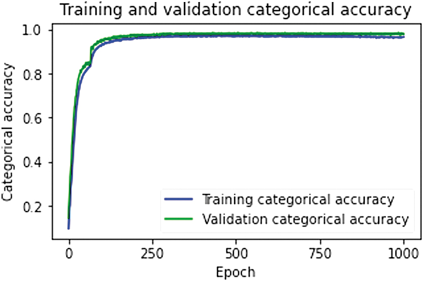
The changes in classification accuracy on the training and validation set.

Uncertainty measurement for the prediction of the BCNN and outlier detection on MNIST dataset

In the last subsection, the architecture of the BCNN that we constructed is confirmed to be sensible. Now, we are going to calculate the epistemic, aleatoric, and misspecification uncertainty, respectively, using Eqs. (9) and (11). Because outlier detection is an unsupervised problem, the model should master all the data. Therefore, we should clear the BCNN model we trained and re-train it with the whole dataset. In general, when the model complexity is fixed, with the increase of data volume, the model accuracy on the test set will rise slowly and that on the training set will not have evident changes as long as the model is not overfitting in the beginning.^4,25

From the experiments of Construction of BCNN section, the results on the training set and the test set are all fine and pretty close, so the possibility of overfitting can be excluded. Moreover, because we only add a little bit more data in this instance, the model performance will hardly change. After re-training, we obtain that the model has high classification accuracy stabilizing ∼97%–98%. In the following experiment, we will also carry out the process like this.

When we call a BNN model every time, it will extract a new sample of network weight ω from the variational posterior to produce the output. Therefore, we call the BCNN 1000 times, which is equivalent to take 1000 samples from q(ω|θ), to estimate the expectation or variance about ω in Eqs. (9) and (11) using MC methods. Figure 2a–cseparately shows the distribution of the epistemic, aleatoric, and misspecification uncertainty generated in the BCNN's predictions for all the observations. We can see, for any kind of uncertainty, the uncertainty of most samples is at a low level, and only a few samples have high uncertainty levels.

FIG. 2.

Different kinds of uncertainties in the predictions of the BCNN model. (a) The epistemic uncertainty; (b) the aleatoric uncertainty; (c) the model misspecification uncertainty; (d) the total prediction uncertainty. BCNN, Bayesian convolutional neural network.

For each kind of uncertainty, we have visualized the images with uncertainty level that reaches the top 1.5%. The selection of the specific value of this percentage is not important. What is crucial is that, for each type of uncertainty, we should grasp the patterns of the images with high uncertainty (for the experiment of Outlier Detection on MNIST Dataset Using BCNN section) or the locations of high uncertainty observations (for the experiment of Outlier Detection on Taxi Dataset Using BLSTMNN section), and their relevance to the outliers that we want. Because MNIST is a quite large dataset, the number of high uncertainty images in each group is at least >1000.

Therefore, there is no enough space to put all of them in this article, but all these images are available to be viewed at our online Github repository.¹⁵ We find that if we use only one of these uncertainties alone to detect outliers, the digits with high uncertainty of each kind are mostly anomalous but there are also some clear digits wrongly classified. Hence, we first normalize each kind of uncertainty (subtract their minimum from them and divide them by their standard deviation), and then add them up to construct the total prediction uncertainty, which is given in Figure 2d. Following the approach in Outlier Detection Using BNNs Based on Uncertainty Measurement section, we choose the uncertainty threshold to be 13 after many trials.

The selection process of this threshold is as follows. To begin with, we select a very large threshold, for example, the 99% quantile of the total prediction uncertainty, and observe the images whose uncertainty level is beyond this threshold. At this moment, most images are anomalous, and then we lower this threshold at a slow pace. During this process, more anomalous images are detected but there are more and more normal images that are misclassified. When a limit state that lowering this uncertainty threshold will mostly bring normal images and only bring few anomalous images is reached, we should stop this process and the threshold at the moment is what we can choose.

After many tests, we find 13 is a suitable threshold that can bring good results. However, it is worth mentioning that the selection of the specific value of the uncertainty threshold is not absolutely strict, which is relatively subjective. The threshold reflects a kind of tolerance in our belief, that is, to what degree can we consider an image to be anomalous, and there is not a definite boundary between normal images and anomalous images.

In total, there are 1228 images classified as outliers, accounting for ∼1.754% of the whole dataset. We select 120 anomalous images and visualize them in Figure 3. A complete display of these abnormal images is available at the online Github repository.¹⁵ We can see except that a few recognizable digits are wrongly classified, most of the images are very vague, or messy, or easy to confuse with other numbers. Overall, the BCNN has a very good performance in outlier detection on MNIST dataset, although with a few errors.

FIG. 3.

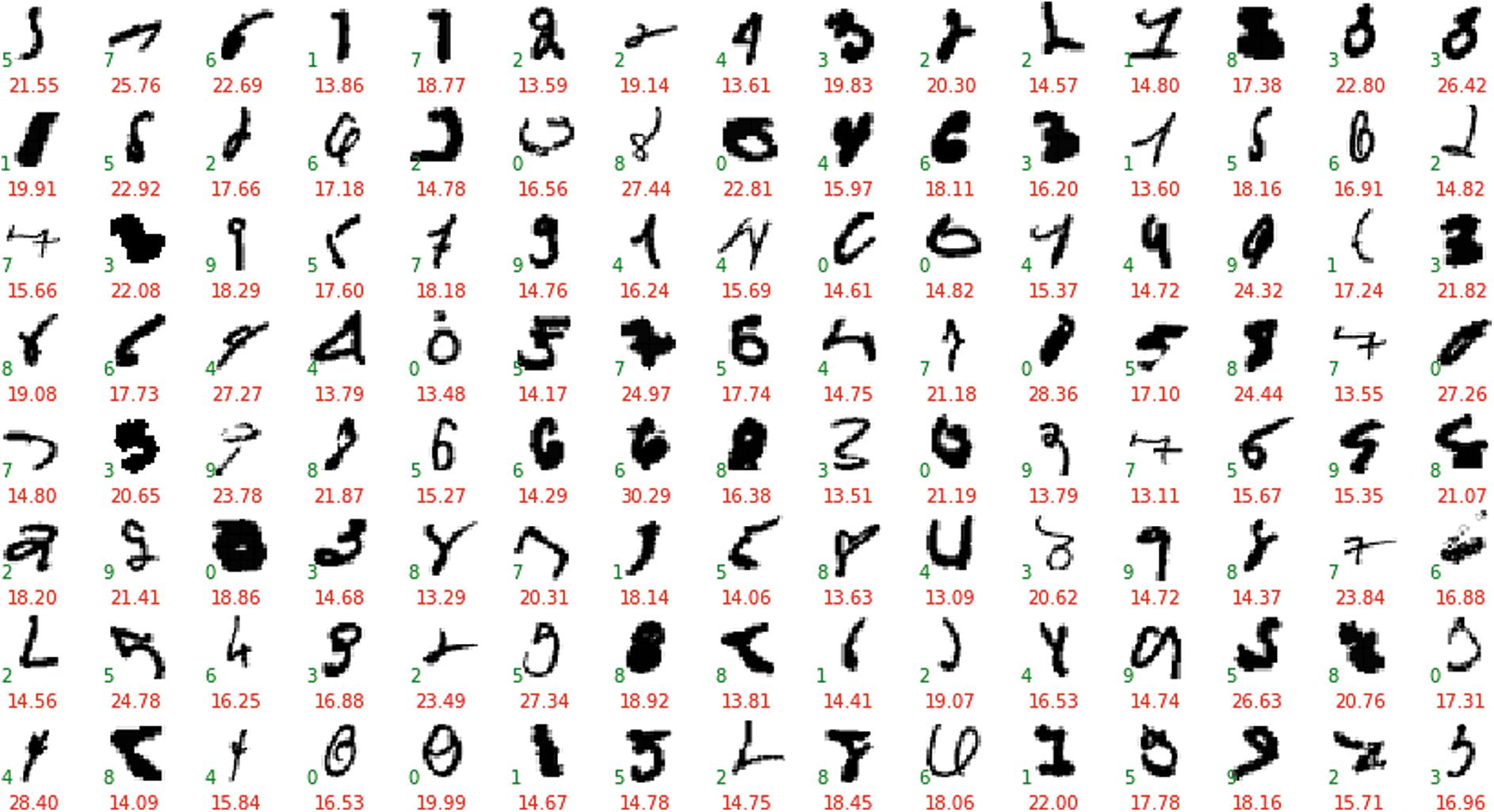
Part of outliers in MNIST dataset detected by the BCNN. MNIST, Modified National Institute of Standards and Technology.

Compared with the methods of using only epistemic or aleatoric uncertainty to detect outliers in other research, such as Refs.,^13,14 our method of using uncertainty combination models not only can effectively reduce the amount of normal images that are misclassified by the network but also has other benefits. In particular, the value of the total prediction uncertainty can excellently evaluate the degree of abnormality of each image and be significantly helpful when we are going to decide which samples are abnormal. In this aspect, the total prediction uncertainty is much more pragmatic and effective than any kind of single uncertainty.

Comparison with LOF and DBSCAN methods on MNIST dataset

LOF method measures the local deviation of the density at a given observation with respect to its neighbors [4, P2421]. The items that have a substantially lower density than their neighbors could be considered as outliers. This method uses a value called LOF to measure the degree of anomaly. The higher this value, the more abnormal the observation is. The class named LOF in Scikit-learn package [4, P2421–P2425] is an implementation of the LOF algorithm. There are mainly two parameters of this algorithm that need to be tuned. One is the threshold of the negative value of LOF below which the observation is classified as an outlier, and the other is the number of the neighbors that the local density of each observation is compared with. DBSCAN is originally a clustering method that finds core samples in high density regions and then expands clusters based on them [4, P1638].

The isolated points that do not belong to any cluster are classified as noisy points and can be regarded as outliers. The class named DBSCAN in Scikit-learn [4, P1638–P1642] is an implementation of this method. For this algorithm, there are also mainly two parameters that need to be adjusted. One is the maximum distance between two samples below which they can be considered as in the neighborhood of each other, and the other is the minimal number of samples in the neighborhood of a point required for it to be considered as a core point. Because of space limitation and that these two methods are not core research objects of this article, we omit the detailed description of the parameter selection process for these two methods here. However, in all the experiments, we had carefully tuned all the parameters to make the results of these two methods as best as possible.

There are totally 356 and 326 images that are classified as outliers by the LOF and DBSCAN methods, respectively, accounting for only 0.509% and 0.466% of the entire dataset, respectively. Figure 4a and b separately displays a part of the images detected by these two methods, which are samples of size 90 taken randomly. The red number beneath each image in Figure 4a represents the value of LOF for each sample. The larger the value, the more confident the LOF method is to classify the corresponding samples into outliers. However, the DBSCAN method cannot show its confidence level when detecting outliers. The complete versions of these images are available at the online Github repository.¹⁵

FIG. 4.

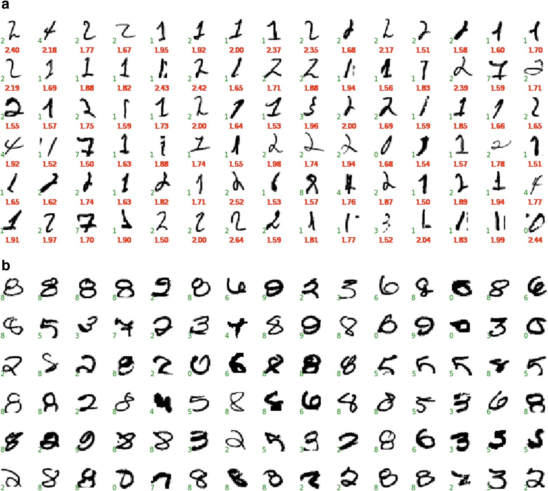
Outlier detection on MNIST dataset using LOF and DBSCAN methods. (a) Part of outliers detected by LOF method; (b) part of outliers detected by DBSCAN method. DBSCAN, Density-Based Spatial Clustering of Applications with Noise; LOF, Local Outlier Factor.

Most outliers detected by LOF are the images with label “1” and “2,” and most outliers captured by DBSCAN are the images with label “8,” followed by the label “2,” “3,” and “5.” Moreover, the images with label “6” or “9” and the images with label “1” are not detected by LOF and DBSCAN, respectively. It means the detection ability of these two methods has evident limitations. Although some images detected by them are illegible or easily confusing, there are many images that are clear to recognize but misclassified by them. Besides, because both algorithms have detected only an extremely tiny minority of the images in the whole dataset, there are a large number of anomalies that are missed by them. Hence, in this experiment, these two methods all have a high misclassification rate and leakage rate.

Overall, compared with the results of the BCNN, the LOF and DBSCAN methods all have a much worse performance on image data. One possible reason is that they do not have the outstanding properties of CNNs in computer vision, such as translation invariance and spatial hierarchy. They can only mechanically compare the difference in each pixel between different images, and cannot recognize the flexible changes in positions and shapes of images.

Outlier Detection on Taxi Dataset Using BLSTMNN

Taxi dataset is sorted from the NYC Taxi and Limousine Commission (TLC) trip record data.²⁶ It is a time series of taxi passengers' counts in New York City in half-hour intervals from July 1, 2014 to January 31, 2015, which has 10,320 observations. The outliers in it are some extremely high or low counts caused by some special events in New York. The working mechanism of LSTMNNs enables them to have memory function, and so they are suitable to process time series data.^{8, Ch6} Hence, we will train a BLSTMNN to predict the counts of taxi passengers in this section. Based on it, the outliers can be detected, and we can discover what the influential events are and the nature of the influence.

Initial data analyses

Figure 5a provides the plot of Taxi dataset. There is a strong seasonal variation but no obvious trend in this series. We need to remove the seasonality at first. Otherwise, the extreme counts that we detect may be caused by peak or valley periods of traffic. We use the classical moving average method²⁷ to estimate the seasonal variation and take the period of the seasonality to be 336 (1 week). This task can be carried out by the Python module statsmodels.tsa.seasonal. Figure 5b provides the plot after removing the seasonality, in which several periods experiencing extreme counts are exposed. The seasonality removal makes our work much easier.

FIG. 5.

The counts of taxi passengers in New York City. (a) Plot of the original data; (b) plot of the data after seasonality removal.

Construction of BLSTMNN

Table 2 provides the structure of the BLSTMNN that we construct. There are two hidden Bayesian LSTM layers, with 8 and 16 U, respectively. The input data are constructed using a sliding window with stride one, where each window contains the data of the time and passengers' counts in the previous 24 time steps (12-hour period). Therefore, the input shape of the BLSTMNN is (24 × 2). The inputs are normalized by the Batch Normalization layer in the beginning. Because time series prediction is essentially a regression task, the outputs are modeled as independent normal distributions with trainable mean and variance. The final dense layer with 2 U is added to, respectively, produce the mean and variance of the normal distribution for each input.

Table 2.

Structure of the Bayesian long short-term memory neural network

Layer	Units	Output shape	Parameter no.
Batch normalization	—	None, 24, 2	8
BLSTM 1	8	None, 24, 8	672
BLSTM 2	16	None, 16	3136
Dense	2	None, 2	34
Independent normal	—	Distribution	0

BLSTM, Bayesian long short-term memory.

The labels to predict are passengers' counts in current time steps. We start from the second time step, and use the first data point to pad the input sequences for the initial 23 steps to keep the length of all the segments be 24. Consequently, 10,319 series segments are constructed as inputs. Then, we split them into training, validation, and test set, accounting for 80%, 10%, and 10%, respectively.

Next, we use RMSprop optimizer to reduce the loss, the negative ELBO (Eq. [4]). Because of slow convergence, we take a large learning rate of 0.5 and train the model for 5000 epochs. In regression scenarios, MSE is often adopted to evaluate the model accuracy.

Figure 6a and b, respectively, provides the changes in the loss and MSE on the training and validation set. After the network is convergent, the MSE for them stabilizes between 3 × 10⁶ and 4 × 10⁶ finally, and for the test set it is 3,677,017.75. By taking the square root, we can obtain the average prediction error of the BLSTMNN at about 1700–2000. Considering that the mean of the passengers' counts is 15,127 after removing the seasonal variation, the average prediction accuracy of the network is ∼87%–89%. In addition, because the error of the prediction to abnormal samples is usually extremely large, the prediction accuracy for regular samples will usually be at least >90%. In consideration of forecasting real-world sequences is quite hard, the results obtained are accurate enough and so the structure of the BLSTMNN that we constructed is sensible.

FIG. 6.

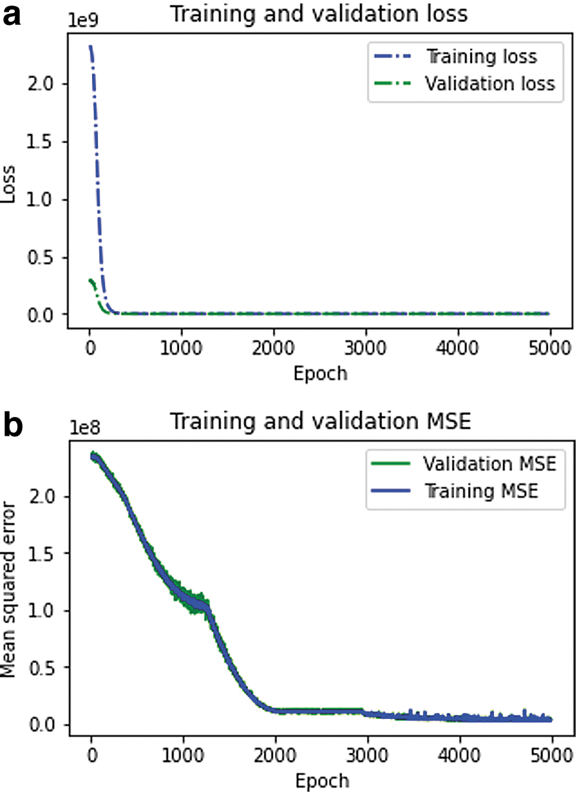
The changes in training and validation loss and MSE for Taxi dataset. (a) Changes in training and validation loss; (b) changes in training and validation MSE. MSE, mean-squared error.

Uncertainty measurement for the prediction of the BLSTMNN and outlier detection on Taxi dataset

We should still clear and re-train our model with the whole dataset. After re-training, the MSE is 3,148,711, which is reasonable. In this instance, we should calculate different kinds of uncertainties using Eqs. (7) and (10). We still call the model 1000 times to estimate the expectation or variance about ω. The distributions of the epistemic, aleatoric, and misspecification uncertainty are given in Figure 7a–c, respectively, which have common characteristics. For any kind of uncertainty, the uncertainty levels for most samples are low but large for some observations, and have a very broad range. The scales of all the uncertainties are much larger than those in the previous experiment because the task of predicting real-world series is much more difficult, where the epistemic uncertainty and the misspecification uncertainty still have the smallest and the largest scales, respectively. Unlike other uncertainties, the distribution of the aleatoric uncertainty does not begin at zero because this kind of uncertainty cannot vanish even if more data are given.

FIG. 7.

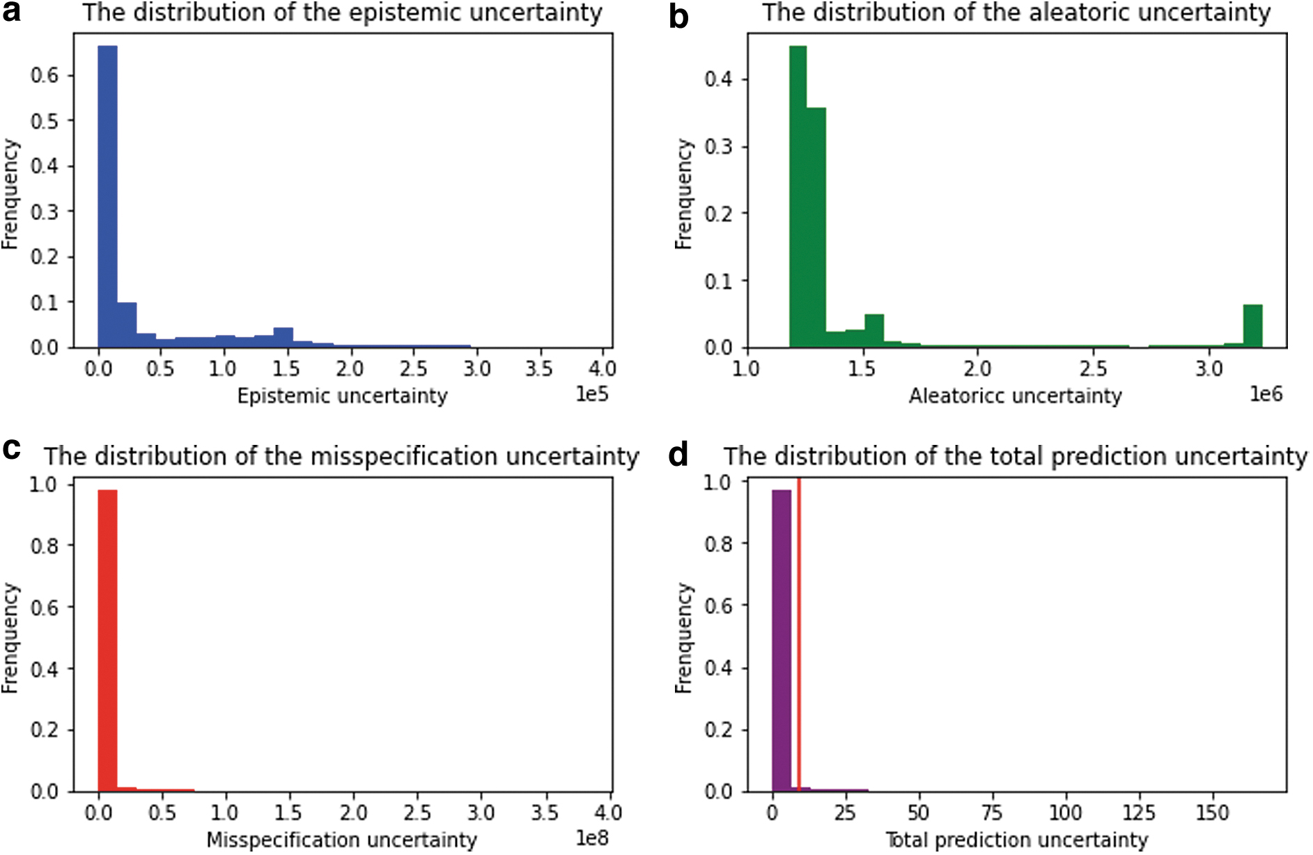
Different kinds of uncertainties in the predictions of the BLSTMNN model. (a) Epistemic uncertainty; (b) aleatoric uncertainty; (c) model misspecification uncertainty; (d) total prediction uncertainty. BLSTMNN, Bayesian long short-term memory neural network.

On this occasion, the outliers are only the samples with extreme labels, which are irrelevant to sample features. The locations of the observations with high epistemic, aleatoric, and misspecification uncertainty are given in Figure 8a–c, respectively. The high uncertainty observations are marked as the red dots and the size of the dots represents the value of the corresponding uncertainty. In this situation, we take the samples whose uncertainty level reaches the top 2.5%. From Figure 8a, we can see the samples with high epistemic uncertainty only correspond to inliers, so we abandon this uncertainty. From Figure 8b, we can see most samples with high aleatoric uncertainty correspond to the outliers with extremely small values, so the aleatoric uncertainty plays a part in this case. Then, from Figure 8c, the samples with high misspecification uncertainty generally correspond to the outliers but there are also some observations that are misclassified.

FIG. 8.

Locations of the observations with high uncertainty in Taxi dataset. (a) Observations with high epistemic uncertainty; (b) observations with high aleatoric uncertainty; (c) observations with high misspecification uncertainty.

Moreover, it can be verified that model predictions are normally accurate for usual samples, but deviate far from extremely large or small samples because the information about these extreme samples is scarce. All in all, model misspecification uncertainty generally plays a chief role in detecting observations with extreme labels. Hence, to sum up, we combine the aleatoric and misspecification uncertainty using Eq. (12) in the following way to construct the total prediction uncertainty: $\begin{matrix} \frac{A l e a t o r i c - m i n (A l e a t o r i c)}{S t d (A l e a t o r i c)} \\ + 6 \times \frac{M i s s p e c i f i c a t i o n - m i n (M i s s p e c i f i c a t i o n)}{S t d (M i s s p e c i f i c a t i o n)} \end{matrix}$ (13)

The term corresponding to misspecification uncertainty is additionally multiplied by six for emphasis. Figure 7d provides the distribution of the total prediction uncertainty for each observation, which has similar characteristics with the three individual uncertainty sources. It is low for most samples but very large for some extreme samples, and it has a wide range. After many trials, we take the threshold as 97.5% quantile of the total prediction uncertainty, which can bring good results.

Figure 9a provides the observations classified as outliers by the BLSTMNN. The size of the red dots stands for the total prediction uncertainty for each observation, which means the larger the dot, the more confident the model is to classify the sample into an outlier. In this figure, we can see the more extreme the dot, the larger its size is, which coincides with our expectation. Almost all the outliers (the extremely large or small values) are detected by the BLSTMNN and there are few points misclassified. Based on these results, we calculate the duration of the periods experiencing extremely high or low taxi passengers' counts, respectively, for each day. The results are given in Figure 9b.

FIG. 9.

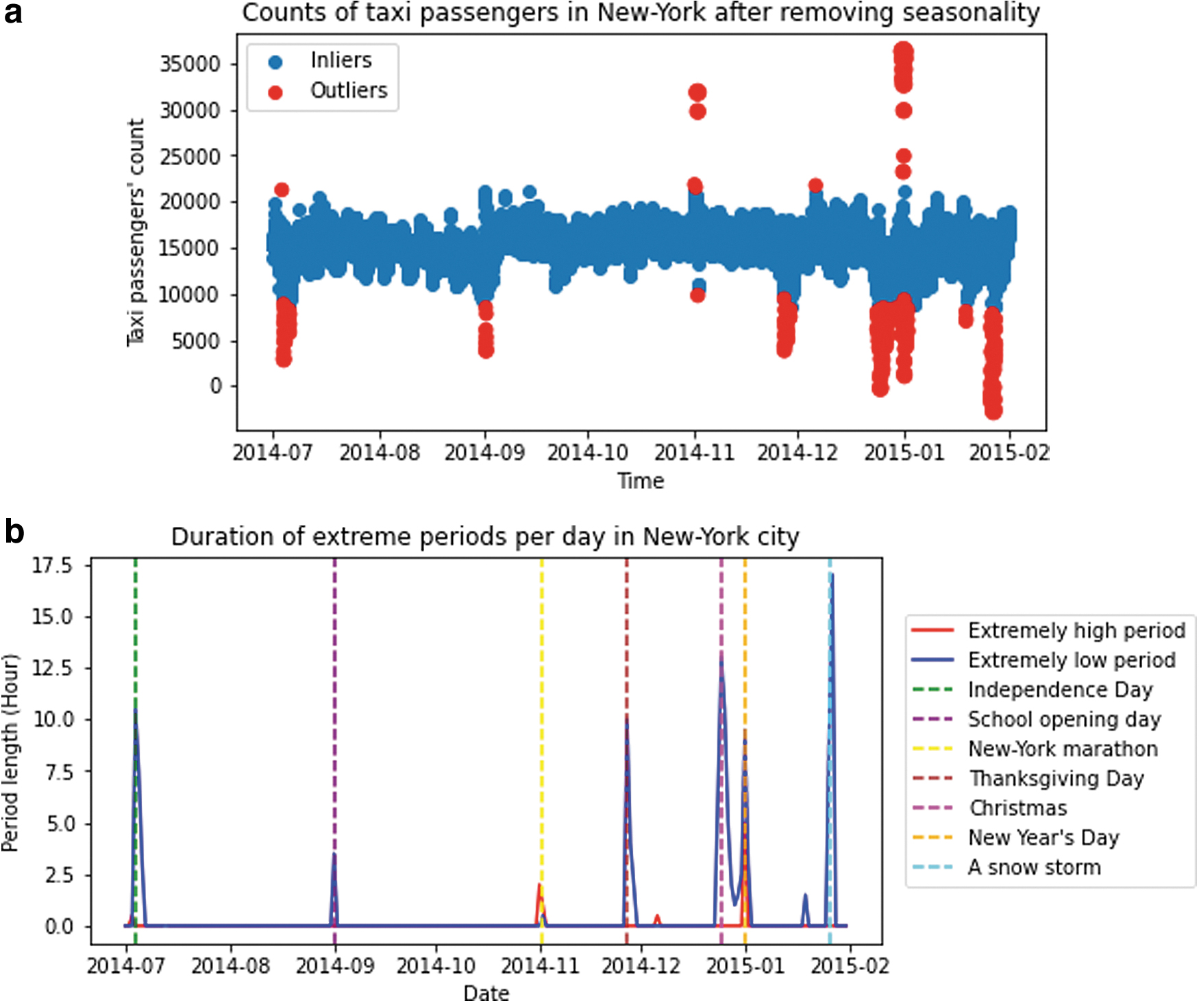
Results of outlier detection on Taxi dataset using BLSTMNN. (a) Observations classified as outliers by the BLSTMNN; (b) duration of the periods experiencing extremely high or low number of passengers.

Furthermore, after consulting the dates of some important events, we can obtain there are totally seven events, American Independence Day, School opening day, the New York marathon, Thanksgiving Day, Christmas, New Year's Day, and a snow storm, that caused a significant influence on the traffic in New York City. Overall, the effects of Christmas, New Year's Day, and the snow storm were the largest. Only the New Year's Day and New York marathon caused an increase in passenger number, whereas all the other events led to a decrease. The New Year's Day was also the sole event that caused both a surge and a significant drop in passenger number in different periods of 1 day. The snow storm was the most influential event, whose negative impact could even last several days after it. Altogether, the BLSTMNN has a very good performance in outlier detection on Taxi dataset.

Compared with the approach of using only one kind of uncertainty each time to detect outliers as in Refs.,^13,14 our method of utilizing combination models can remarkably improve the detection effect. According to Figure 8a, if only epistemic uncertainty is used as in Pawlowski et al,¹³ the results that we obtained will be totally wrong. From Figure 8b, all the extremely large values as well as many extremely small values will be missed if only aleatoric uncertainty is used. Comparing Figures 8c and 9a, we can find that using uncertainty combinations can further reform the outcomes compared with using only misspecification uncertainty. The amount of normal observations that are misclassified is notably reduced when appropriate combination of different kinds of uncertainties is adopted.

Comparison with LOF and DBSCAN methods on Taxi dataset

Finally, let us investigate the effects of LOF and DBSCAN methods. Figure 10a and b, respectively, provides the results of these two methods. The size of the red dots in Figure 10a represents the value of LOF for each observation, which has similar meaning with that in Figures 8 and 9a. As illustrated in Comparison with LOF and DBSCAN Methods on MNIST Dataset section, all the experimental results of the LOF and DBSCAN methods discussed here are still based on the fact that the parameters of both algorithms had been carefully tuned to make the results as best as possible. The LOF method can detect the observations with extremely large values, but fails to detect most samples with extremely small values. In addition, many points at the edge of the cluster that should not be outliers are marked as anomalies by this method.

FIG. 10.

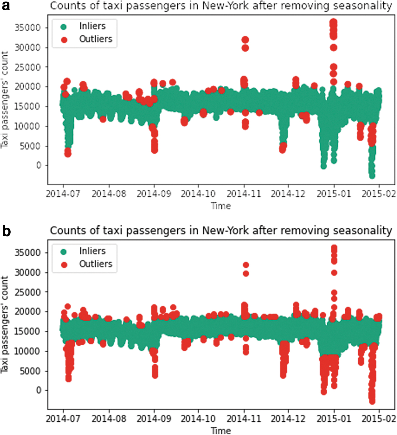
Outlier detection on Taxi dataset using LOF and DBSCAN methods. (a) Outlier detection with LOF method; (b) outlier detection with DBSCAN method.

Hence, the LOF method has a poor performance on this time series dataset. The performance of the DBSCAN method is much better. It can detect both extremely large and small observations. However, too many points at the edge of the cluster that should not be extreme values are also classified as outliers by DBSCAN. All in all, the performances of these two methods on Taxi dataset are all inferior to BLSTMNN to varying degrees.

Conclusions

The main objective of this article was to develop a general outlier detection method using BNNs based on uncertainty measurement. We adopted the methods in Zhu and Laptev⁹ to measure epistemic and aleatoric uncertainty, but in classification scenarios, we opted for a variant of the method in Chen et al,¹⁴ the probability entropy, to quantify aleatoric uncertainty. For model misspecification uncertainty, there is no practical quantification method at present. Thus, we proposed a new method of utilizing the value of loss function to quantify it. This value can indicate the level of uncertainty about whether an observation comes from a different distribution than the cluster of training data. Then, total prediction uncertainty can be obtained by the combination of these three uncertainty sources, and linear combinations were adopted in this article. It measures the model's confidence to classify a sample into an outlier (or the anomaly degree of observations).

Afterward, to apply this method in outlier detection on different types of data, we, respectively, trained a BCNN classification model for MNIST dataset and a BLSTMNN regression model for time series prediction on Taxi dataset. We find that if the network wonderfully suits the data and different uncertainties are combined reasonably, the observations with high total prediction uncertainty generally correspond to outliers in the data. Furthermore, we compared this method with the BNN anomaly detection methods proposed previously in Refs.^13,14 whose core idea is to merely use a single index that corresponds to only epistemic or aleatoric uncertainty to detect outliers each time, and the classical LOF and DBSCAN methods.

The results demonstrate that, compared with the methods of Refs.,^13,14 our method of using uncertainty combinations not only can obviously reduce the model's misclassification rate on outliers, but also has the benefit that the value of total prediction uncertainty can better depict the anomaly degree of an observation. Moreover, the performance of our method is also superior to the LOF and DBSCAN methods in each experiment to varying degrees. To the best of our knowledge, this research is the first time to consider the relationship between the essential classification of various uncertainties and the outliers in the data, and suggest to adopt combination models on different uncertainty sources to improve the effects of anomaly detection models.

Discussion

In this article, we demonstrate that BNNs can achieve a good effect in outlier detection. However, we do not have enough evidence about whether this method can be applied in novelty detection, that is, whether BNNs can detect outliers in new data. On the contrary, for anomaly detection problems, there is no general method presently to detect different kinds of anomalies separately. For example, in both regression and classification, there are two kinds of anomalies. One is that the samples with usual features have anomalous labels, the other is that the samples have extreme features. It is a quite difficult task to capture them separately.

Future work should aim to make breakthroughs to these limitations. More experiments of using BNNs to perform novelty detection on different types of data should be conducted. We should explore whether the predictions of BNNs to new data are reliable and whether the uncertainties for these predictions can measure the anomaly degree of the new data. Besides, to capture different types of anomalies separately, we can consider finding other effective ways to combine different kinds of uncertainties together (may be nonlinear combination) such that the samples with high total prediction uncertainty just correspond to the kind of anomaly that we want.

Footnotes

Author Disclosure Statement

No competing financial interests exist.

Funding Information

No funding was received for this article.

Abbreviations Used

One-Hot Encoding and One-Hot Categorical Distribution

One-hot encoding, also called one-bit effective encoding, uses N-dimensional vector to encode N classes. Assume X is a discrete random variable, which takes N possible values (or belongs to N possible classes). Without loss of generality, we use labels 1,2,…,N to denote these values or classes. Assume H is a N-dimensional vector. Then, we call H the one-hot encoding of X if the following conditions are satisfied:

(1) The elements of H can only take two possible values, 0 or 1;

(2) At any time, H has and only has one element that takes value 1 and all the other elements of H take 0;

(3) The k-th element of H takes 1 if and only if X takes the value with label k (or belongs to the k-th class) ( $k = 1, 2, \dots, N$ ).

One-hot categorical distribution is a generalization of Bernoulli distribution to the situation of multiple classes. Further assume the probability that random variable X takes the value with label k (or belongs to the k-th class) is p_k, where $0 \leq p_{k} \leq 1$ , k = 1,2,…,N and $\sum_{k = 1}^{N} p_{k} = 1$ . Assume the N-dimensional vector H is the one-hot encoding of X. Then, H is a random vector. Let p = (p₁, p₂,…,p_N). We call that H follows the one-hot categorical distribution with probability vector p, and denote it as $H \sim O n e H o t C a t e g o r i c a l (p) .$

References

Khan

, Foley

, O'Sullivan

. Database intrusion detection systems (DIDs): Insider threat detection via behavioural-based anomaly detection systems—A brief survey of concepts and approaches. In: 2021 International Symposium on Emerging Information Security and Applications. Springer, 2021. pp. 178–197.

Nagaraja

, Soumya

, Sinha

, et al. Fake news detection using machine learning methods. In: 2021 International Conference on Data Science, E-learning and Information Systems, 2021. pp. 185–192.

Moschini

, Houssou

, Bovay

, et al. Anomaly and fraud detection in credit card transactions using the ARIMA model. In: Engineering Proceedings, volume 5. Multidisciplinary Digital Publishing Institute, 2021. p. 56.

Pedregosa

, Varoquaux

, Gramfort

, et al. Scikit-learn User Guide, 0.23.2 edition, August 2020. Available online at scikit-learn.org/0.23//_downloads/scikit-learn-docs.pdf (last accessed October 6, 2021).

Breunig

, Kriegel

, Ng

, et al. LOF: Identifying density-based local outliers. In: Proceedings of the 2000 ACM SIGMOD International Conference on Management of Data, 2000. pp. 93–104.

Ester

, Kriegel

, Sander

, et al. A density-based algorithm for discovering clusters in large spatial databases with noise. In: KDD, volume 96, 1996. pp. 226–231.

Liu

, Ting

, Zhou

. Isolation forest. In: 2008 Eighth IEEE International Conference on Data Mining. IEEE, 2008. pp. 413–422.

Chollet

Deep learning with python, volume 361. New York: Manning, 2018.

Zhu

, Laptev

. Deep and confident prediction for time series at

Uber

. In: 2017 IEEE International Conference on Data Mining Workshops (ICDMW). IEEE, 2017. pp. 103–110.

10.

Kendall

, Gal

. What uncertainties do we need in Bayesian deep learning for computer vision?. arXiv preprint arXiv: 1703.04977, 2017.

11.

Kwon

, Won

, Kim

, et al. Uncertainty quantification using Bayesian neural networks in classification: Application to biomedical image segmentation. Comput Stat Data Anal. 2020; 142:106816.

12.

Lakshminarayanan

, Pritzel

, Blundell

. Simple and scalable predictive uncertainty estimation using deep ensembles. Adv Neural Inform Process Syst. 2017; 30:6403–6414.

13.

Pawlowski

, Jaques

, Glocker

. Efficient variational Bayesian neural network ensembles for outlier detection. arXiv preprint arXiv: 1703.06749, 2017.

14.

Chen

, Pi

, Wu

, et al. Imbalanced satellite telemetry data anomaly detection model based on Bayesian LSTM. Acta Astron. 2021; 180:232–242.

15.

Tao

Github Repository: Applications of BNNs in Outlier Detection. Available online at https://github.com/TAO-Chen632/Applications-of-BNNs-in-Outlier-Detection.git (last accessed October 6, 2021).

16.

Blei

, Kucukelbir

, McAuliffe

. Variational inference: A review for statisticians. J Am Stat Assoc. 2017; 112:859–877.

17.

Blundell

, Cornebise

, Kavukcuoglu

, et al. Weight uncertainty in neural network. In: Proceedings of the 32nd International Conference on Machine Learning, volume 37. PMLR, 2015. pp. 1613–1622.

18.

Bishop

CM.

Pattern recognition and machine learning, 1st ed, volume 4. New York: Springer, 2006.

19.

Hinton

, Van Camp

Keeping the neural networks simple by minimizing the description length of the weights. In: Proceedings of the Sixth Annual Conference on Computational Learning Theory, 1993. pp. 5–13.

20.

Barber

, Bishop

. Ensemble learning in Bayesian neural networks. Nato ASI Series F Comput Syst Sci. 1998; 168:215–238.

21.

Salama

Probabilistic Bayesian Neural Networks: Building probabilistic Bayesian neural network models with TensorFlow Probability. Available online at https://keras.io/examples/keras_recipes/bayesian_neural_networks/ (last accessed April 8, 2022).

22.

LeCun

, Cortes

, Burges

CJC

. The MNIST database of handwritten digits. Available online at http://yann.lecun.com/exdb/mnist/ (last accessed October 6, 2021).

23.

LeCun

, Bottou

, Bengio

, et al. Gradient-based learning applied to document recognition. Proc IEEE. 1998; 86:2278–2324.

24.

Gelman

, Carlin

, Stern

, et al. Bayesian data analysis. Chapman and Hall/CRC texts in statistical science, 3rd ed. Boca Raton, FL: CRC Press, 2015.

25.

VanderPlas

Python data science handbook: Essential tools for working with data, 1st ed. Sebastopol, CA: O'Reilly Media, Inc., 2016.

26.

NYC Taxi & Limousine Commission. TLC trip record data. Available online at https://www1.nyc.gov/site/tlc/about/tlc-trip-record-data.page (last accessed October 6, 2021).

27.

Aryness

, Woodlief

. The use of moving averages in the measurement of seasonal variations. J Am Stat Assoc. 1928; 23:241–252.