




Abstract
With the development of automatic electrical devices in smart grids, the data generated by time and transmitted are vast and thus impossible to control consumption by humans. The problem of abnormal detection in power consumption is crucial in monitoring and controlling smart grids. This article proposes the detection of electrical meter anomalies by detecting abnormal patterns and learning unlabeled data. Furthermore, a framework for big data and machine learning-based anomaly detection framework are introduced. The experimental results show that the time series anomaly detection for electric meters has better results in accuracy and time than the expert alternatives.
Introduction
The old power grid infrastructure that supplies power to users has been being replaced in recent years by a succession of digital systems known as smart grids. Consumers and utility providers will benefit immensely from this upgraded grid's ability to monitor, control, and forecast energy consumption. The data of energy consumption are time series form. Learning temporal patterns in time series has remained a complex problem. It is critical to understand the underlying structure of a system's normal behavior, especially when detecting anomalies in time series.1–3
The electrical consumption data are first deconstructed to emphasize the seasonal, trend, and random features. The seasonal component captures the electrical consumption data fluctuation over each day, which is repeated throughout the breakdown. The trend component displays any observed data departures from the trend component and seasonal component data in aggregate, whereas the random component displays any observed data deviations from the trend component and seasonal component data in aggregate. In the case of electrical data, the decomposition is comparable. The trend component represents the magnitude of the consumption, 340 kWh. The trend component looks to move a lot on the graph, although its variability over the week interval is less than 2%.3–5
To handle the challenge of anomaly detection with time series data, a variety of anomaly detection techniques have been developed. Table 1 outlines some of the specific approaches and case studies in anomaly detection studies with time series. One of the most challenging problems in anomaly detection is the problem of limited data. Labeled data are scarce, whereas unlabeled data are abundant. Positive unlabeled learning (PUL) is a recommended method to solve this problem. Table 2 summarizes some of research that have used PUL to handle data imbalance and missing data issues. Symbolic aggregate approximation (SAX) is a method that transforms a time series into discrete symbolic sequences. It is widely used in many subjects such as pattern recognition and anomaly detection. Some research on SAX is summarized in Table 3. The study by González-Vidal et al. 6 used Heuristically Order Time series using SAX algorithm to detect anomalies in water management. Trend symbolic aggregate approximation 7 and symbolic aggregate approximation - change points (which captures the trends in a time series based on abrupt Change Points [CP]) 8 are new SAX techniques and improve performance in classification. Symbolic aggregate approximation in time series researches are summarized in Table 3.
Abnormal detection in time series researches
LGB, Light Gradient Boosting.
Positive unlabeled learning researches
ANN, artificial neural networks; LP-PUL, Label Propagation for Positive Unlabeled Learning; LR, logistic regression; MNIST, Modified National Institute of Standards and Technology; OCSVM, one-class support vector machine; PUL, positive unlabeled learning; PURE, Positive-Unlabeled Reconstruction Encoding; SVHN, street view house numbers; USPS, U.S. postal service.
Symbolic aggregate approximation in time series researches
ARIMA, Autoregressive Integrated Moving Average; ECG, electrocardiography; HOT-SAX, Heuristically Order Time series using SAX; SAX-CP, symbolic aggregate approximation - Change Points; TSAX, trend symbolic aggregate approximation.
This article aims to detect anomalous electric meters automatically by using abnormal behavior pattern detection and unlabeled learning method. Specifically, combine two methods multiple symbolic aggregate approximation and decompose time series to analyze abnormal behavior. However, most of the data are unlabeled. For anomaly detection, we need an unlabeled learning method to increase the model's accuracy.
The article is organized into four sections: The Methodology section shows the methodology of anomaly detection, multiple SAX, imbalance, and proposed model. The experiments and results of smart meter sensor are shown in the Experiments and Results section. Finally, the conclusion and discussions are provided in the Conclusions and Summarize section. Some acronyms used in the manuscript are given in Table 4.
Table of nomenclature
Methodology
Anomaly detection formula problem
In this article, an energy meter is a sensor that measures the automatic electricity load of a consumer by time. 9 This sensor is binary classified into the anomaly and normal. If the sensor has anomaly status, it will inspect and check. 10
Sensor data set has an input with N features:
Consider the data of a sensor
Overview anomaly detection system
The research procedure of time series anomaly detection system contains four phases:
Phase 1: Integrating Data: Gathering data from various sources and combining it into one data set. Phase 2: Preprocessing Data: Raw data collected from the previous step can be in various formats and may be inconsistent. This step involves data cleaning and data normalization, and features generation is conducted to overcome this problem. Phase 3: Modeling: Processed data set will be split into two sets: a training set and a test set. The training set will be used to train a classifier. Phase 4: Evaluation: This step assists in selecting the best model that meets a set of criteria and evaluating the model's future performance. If the model's performance is poor, go back to the data preprocessing step to clean data and generate more predictive features or the modeling step to tuning the model's hyperparameters.
Decompose time series
Data
where
mt is trend component that is identified by moving average
d is period of seasonal, seasonal component is
rt is residual component. The decomposed components of the time series create new features for data.
Multiple SAX
The approach of SAX converts a time series into discrete symbolic sequences. 11 It is frequently employed in a variety of fields, including pattern recognition and anomaly detection.7,12
A time series of any length N can be reduced to a string of any length
A new method to find the normal pattern of multiple windows
Step 1: Consider a time series of length N:
Step 2: Select a fixed size of window
Thus, the original data now are represented by Mi window
The normal symbolic pattern for data in window
Step 3: Let set 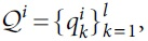 , where
Step 4:
Each symbolic vector has w positions that run from 1 to w. The set of all symbolic at position j of M symbolic vector has form
The meaning
Step 5: After
where
Figure 1 shows an example of using SAX to encode time series. The subsequences of raw time series data in window w are encoded into a symbolic vector using SAX. Figure 2 shows the symbolic anomaly vector using SAX. The anomaly vector is very different from the normal behavior of sensors.
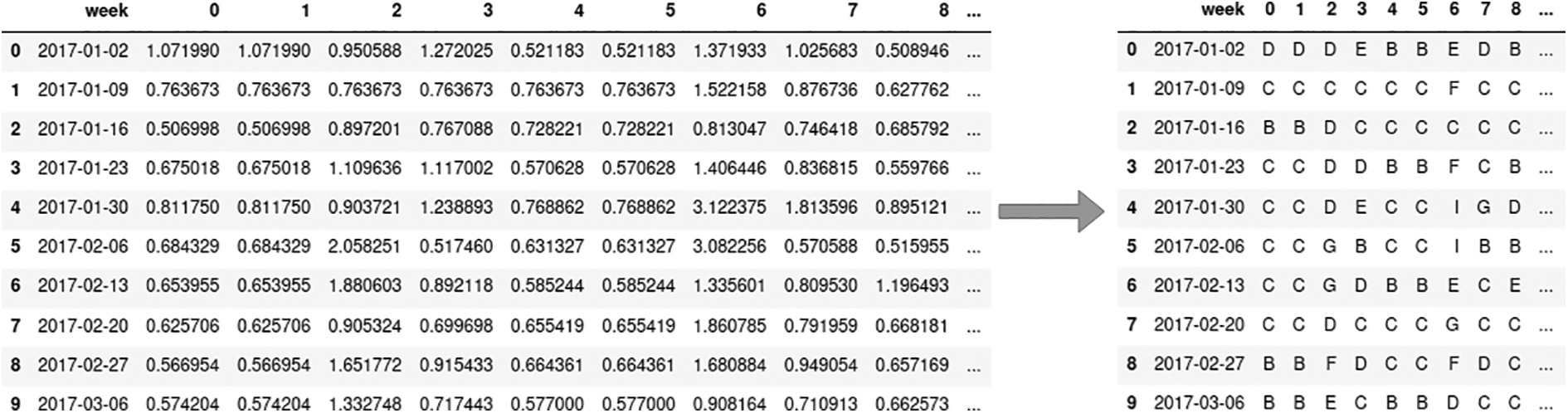
SAX encodes subsequence time series in window w into symbolic vector. SAX, symbolic aggregate approximation.

Extract symbolic anomaly vector using SAX.
It was using this distance for analyzing the new features of two normal and anomaly classes. The advantage of SAX is tolerated noise of time series data a and its variance is small, but it cannot detect abnormal subsequence of w time step.
Positive unlabeled learning
For classification, PUL is a method of learning from a data set labeled positive (Po) and an unlabeled data set (U), where U includes both positive and negative labels.13,14 In the collection U, there is a positive label.
Two-step strategy, the direct approach using the Biased—support vector machine (SVM) algorithm, and probability estimation are the approaches to tackling the PUL problem.
Two-step technique
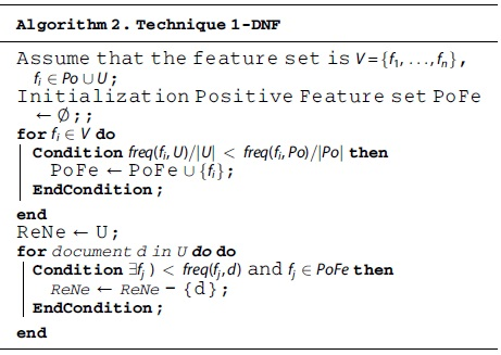
Step 1: From an unlabeled set U, create a trustworthy, Reliable Negative set (notion ReNe). Spying techniques, 1-dynamic noise filter (DNF) procedures, and other methods are utilized to determine the set of reliable negative sets.
Step 2: Create a classifier for the U-ReNe collection using Po and reliable negative. Classifiers such as Iterative SVM, Random Forest (RF), and others are available as options.
Techniques for Spying:
- Random sampling
- Build classifier with new set Po and new U
- Extract the reliable negative set from the above classifier
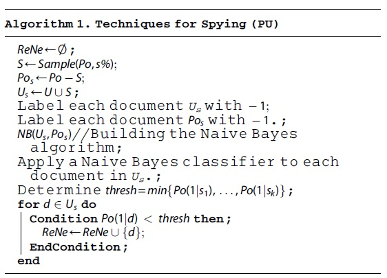
Technique 1-DNF:
Find features that appear more frequently in the set Po than that in the set U
Extract the document in the set U that does not contain the features in the set above. Those documents are high reliable negative documents (ReNe).
In the second step, building a classifier to split the set
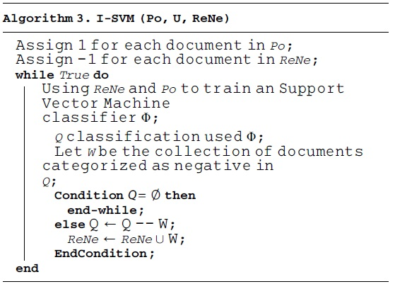
Algorithm Iterative SVM:
- Run the SVM algorithm iteratively using the set Po, ReNe,
Direct approach: biased-SVM
Given the training data set  is one input feature vector and
No noise: The set P has no noise, but the set U does. In this case, according to the SVM formula, we have:
Minimize:
Constrains:
where
In case of noise: In practice, the set P may contain several negative labels. Therefore, we allow noise in the set P, we use soft margin SVM for biased-SVM where the two parameters
Minimize:
Constrains:
The learning process of the biased-SVM algorithm is the process of calculating the inverse derivative to find b.
Building a classifier using probability estimation
This is a probability formula-based approach. Let
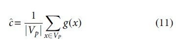
The main goal is to find a classifier function
Here,
For learning, the training set consists of two subsets, the labeled set P
The fixed value
Proposed model
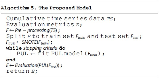
The data set of sensors includes cumulative time series, which represents power consumption per unit time. The proposed model consists of five main parts. Data ingestion: Integrate input data, collect data from electricity meters.
Preprocessing: Includes components that normalize data, removes extraneous data, adds missing data, normalizes data to the same format. Then, normalizes them based on the time period per day.
Feature engineering: Transferring data using the multiple SAX method. Using analysis of time series data by decomposing time series with components: trend, multiseasonal, and residual. These components make up the properties of the electric meter.1,15
Data exploration: The data are divided into train and test sets. Apply imbalance processing techniques for the train set. Then, it is trained using the PUL method with a selected hyperparameter. We evaluate and choose a trained model with an optimized hyperparameter.
Evaluation: Evaluate the results achieved. If the stopping condition is satisfied, the model is learned. If the stopping condition is not satisfied, we will relearn the model with other parameters. Finally, give the results.
We visualize output and test final model by using evaluation metrics. The overview model of this approach is shown in Algorithm 5 and Figure 3, respectively.

Proposed model anomaly detection using machine learning and pattern recognition.
Experiments and Results
Data set description
The data set contains the time series data of cumulative energy of 1067 sensors from January 1, 2017, to March 31, 2018, in a province of Vietnam. The data include about 2.5 million rows, and 3 attributes are described in Table 5:
The description of data set
KWH, kilowatt hours.
Evaluation metrics
Four measures were used in our experiments to evaluate four methods: classification accuracy, Precision, Recall, and F1 score. These criteria are calculated by the following formula:
where:
True Positive (TP) and True Negative (TN) are the proportion of correct classification that positive and negative class data points, respectively.
False Positive (FP) and False Negative (FN) are the proportion of incorrect classification that positive and negative class data, respectively.
Receiver operating characteristic curve
A receiver operating characteristic (ROC) curve of two components: true positive rate (TPR) and false positive rate (FPR). ROC is a graph that displays a classification model across all categorization levels.
TPR or Recall is defined as follows:
FPR has a form:
An ROC curve is used to depict TPR and FPRs multiple categorization criteria. More items are categorized as positive as the classification threshold is lowered, leading to a rise in both False Positives and True Positives.
Area under the ROC curve
The area under the ROC curve (AUC) is a two-dimensional representation of the area beneath the complete ROC curve. The AUC is a separability metric, whereas the ROC is a probability curve. The AUC measures how accurately the model predicts 0 classes as 0 and 1 classes as 1. The better the model predicts 0 courses as 0 and 1 classes as 1, the higher the AUC. The AUC, however, indicates how well the model discriminates. An illustration of the AUC is shown in Figure 4.
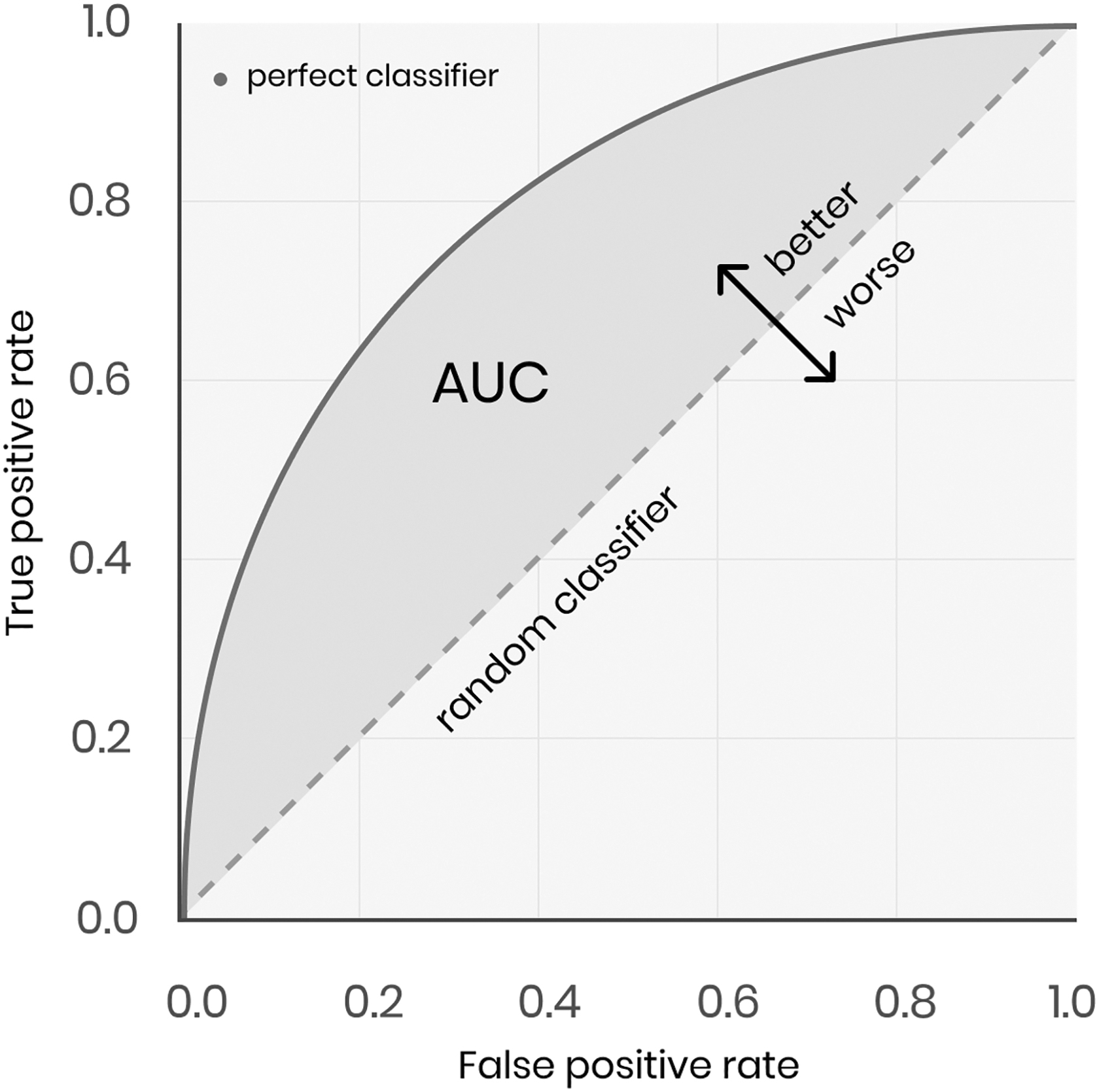
AUC (area under the ROC curve). ROC, receiver operating characteristic.
Results
We use two scenarios for the experiment, there are as follows:
Scenario 1: We use some algorithms such as RF, Decision Tree (DT), LightGBM, and XGBoost to build classifiers to classify data consumption with the features extracted by multiple symbolic aggregate approximation.
Scenario 2: We use the proposed model using multiple symbolic aggregate approximation to extract features, and PUL combined with some classifiers as RF, DT, LightGBM, and XGBoost to build classifiers to classify data.
We use two scenarios to compare the performance of our proposed method with some base classifiers. We run the model 30 times and evaluate the outcomes using the following metrics: mean (


Comparison with state-of-the-art using the original imbalanced data set
The bold values signifies the best performance.
AUC, area under the ROC curve; ROC, receiver operating characteristic.
The results of the scenarios are described in Table 6. Overall, the results when using PUL in combination with the classifiers give better results than when using the separate classifiers. The F1 score result is around 4.3% higher when utilizing PUL with DT. Similarly, when positive unlabeled (PU) is combined with DT, LightGBM, XGBoost, and RF, the F1 score increases by 4.4%, 4.7%, 7.3%, and 20.7%, respectively. It can be shown that when PUL is combined with RF, the generated F1 score results differ the most. The results in Table 6 also show that the results when using PU in combination with the classifiers are more stable than when using the separate classifiers. Figures 7–10 show a box plot showing the results of AUC and F1 score for 30 distinct runs when using the two scenarios.
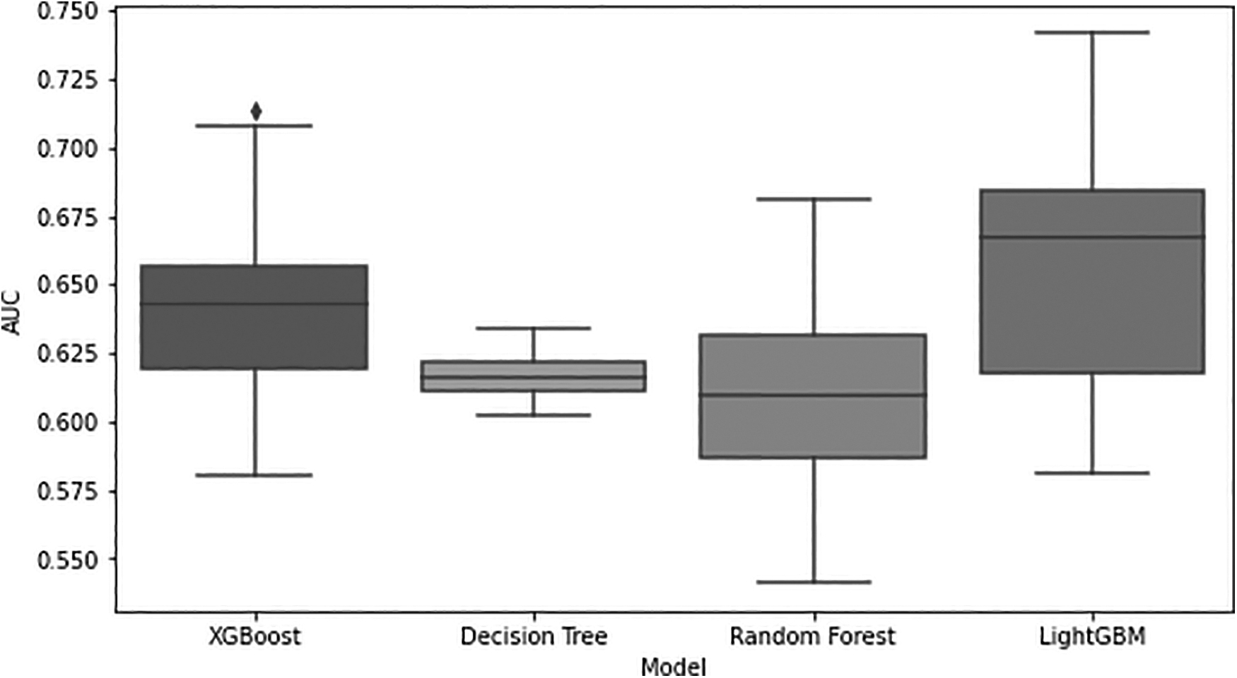
Evaluation metric AUC score of four classifiers.

Evaluation metric F1 score of four classifiers.

Evaluation metric AUC score of proposed model with four classifiers.

Evaluation metric F1 score of proposed model with four classifiers.
The time to training model when using the two scenarios is shown in Table 7. When using PUL with classifiers, time to training model is higher about 20 times than using the separate classifiers.
Time to training model of the two scenarios
Conclusions
A new proposal model combining SAX, handling data imbalance and RF for anomaly detection sensor system are addressed in our research. Concretely, the contributions of our article are as follows:
Successfully using multiple SAX for time series data to find complex and dynamic anomaly patterns.
Archiving applied anomaly pattern for machine learning model.
Fitfully proposed a model combining multiple SAX, imbalance technique, and RF to anomaly detection.
Achieving applied proposal model in automatic meter intelligence system in Vietnam.
According to the experimental result, our proposed model has better performance than using well-known machine learning models. The cause of better results is chosen complex and dynamic anomaly patterns in meter intelligence systems.
In future work, more sensor anomaly detection applications will be researched based on the proposed model. The advanced SAX to find a new pattern will be investigated. The anomaly detection of subsequent symbolic normal patterns is necessary to study.
Footnotes
Authors' Contributions
N.T.N.A. contributed to conceptualization (lead), methodology (lead), software, and writing. V.H.T. was in charge of writing—original draft, software development, formal analysis, visualization, and validation. D.K. and D.M.T. were in charge of conceptualization (supporting), writing—original draft (supporting), writing—review and editing, and investigation. L.A.N. was in charge of methodology, investigation, supervision, and writing—review and editing.
Author Disclosure Statement
No competing financial interests exist.
Funding Information
This research was supported by Energy Cloud R&D Program through the National Research Foundation of Korea (NRF) funded by the Ministry of Science, Information and Communication Technologies (2019M3F2A1073387). In addition, this work is partly supported by the research project number DHFPT/2022/27 granted by the FPT University.